curvature effect on patterning dynamics on spherical...

Universita degli studi di Padova

Dipartimento di Fisica e Astronomia “Galileo Galilei”

Corso di Laurea in Fisica

Tesi di Laurea

Curvature effect on patterning dynamicson spherical membranes

Candidato: Leonardo Pacciani

Relatore: Prof. Enzo Orlandini

Anno accademico 2014-2015

To my family

Abstract

The aim of this thesis is to carry out an analytical study of the role that surfacecurvature may have on the evolution and selection of patterns seen as solutionsof a set of reaction-diffusion equations defined on spheres. Such equations exhibitdiffusion-driven instability of spatially uniform structures leading to spatially non-uniform textures such as coat markings of animals and pigmentation patterns onbutterfly wings. While the case with planar domains has been thoroughly studied inthe past, much less is known for reaction-diffusion equations defined on closed sur-faces. Here we will consider the simpler case of spherical domains, and by describingthe possible stationary solutions in terms of spherical harmonics, we will perform alinear stability analysis of the equations as a function of the radius R of the sphere(i.e. its curvature) and look for the most stable set of patterns compatible with thatradius.

Preface

One of the most challenging questions in biology is the mechanism by which spatialpatterns form in biological contexts; this process is called spatial patterning, and theunderlying physical process is often modelled as the evolution of reaction-diffusionsystems, namely chemical systems in which one or more reagents diffuse within adomain.The study of how spatial patterns can form has many applications in a variety ofbiological fields, e.g. developmental biology, the dynamics of bacterial colonies, orbehavioural aspects of territoriality in particular prey-predator systems. In partic-ular, in developmental biology the properties of the mechanisms that involve theformation of spatial patterns have been used to describe the processes that lead tothe formation of coat markings, or in general skin pigmentation, in animals, whilein morphogenesis (a branch of embryology) they are a key concept in order to un-derstand how an embryo can undergo cell differentiation and thus develop from ahomogeneous spherically symmetric system to a complex organism. From this pointof view, the study of spatial patterning on spherical surfaces is particularly relevant.Even though the study of spatial patterning has shed light on different biologicalissues, many aspects of these processes are still not fully understood. For example,the mechanism that links genes and patterns, namely the way by which geneticinformation is physically translated into patterns and form during the developmentof an embryo, is one of those issues, although recent studies have given interestinghints on particular cases (see [3]).It is thought that the formation of patterns occurs when the concentration of par-ticular chemical substances, generally referred to as morphogens, exceeds a criticalthreshold level (prepattern theory). In other words, cells are thought to be “prepro-grammed” to react to the morphogen concentration, and differentiate accordingly.Thus, we can try to understand how such processes take place studying the spon-taneous evolution of chemical reagents from a homogeneous to an inhomogeneousstate; when this happen we say that the system exhibits diffusion-driven instability.In particular, we say that a system exhibits diffusion-driven instability, or Turinginstability, when its homogeneous steady state is linearly stable in the absence ofdiffusion, but becomes unstable to spatial perturbations when diffusion is present.

vii

Contents

1 Introductory study 11.1 Introduction . . . . . . . . . . . . . . . . . . . . . . . . . . . . . . . . 11.2 General conditions for Turing instability . . . . . . . . . . . . . . . . 2

1.2.1 Mathematical formulation of the problem . . . . . . . . . . . . 21.2.2 Linear stability of the homogeneous steady state . . . . . . . . 31.2.3 Linear instability of the steady state with diffusion . . . . . . 4

1.3 Turing space . . . . . . . . . . . . . . . . . . . . . . . . . . . . . . . . 61.3.1 Determination of Turing space . . . . . . . . . . . . . . . . . . 71.3.2 Representation of Turing space . . . . . . . . . . . . . . . . . 91.3.3 Notes on Turing space . . . . . . . . . . . . . . . . . . . . . . 9

2 Gierer and Meinhardt’s system on a sphere 132.1 Initial considerations . . . . . . . . . . . . . . . . . . . . . . . . . . . 132.2 The role of curvature . . . . . . . . . . . . . . . . . . . . . . . . . . . 16

2.2.1 The effects of curvature . . . . . . . . . . . . . . . . . . . . . 162.2.2 Mode selection . . . . . . . . . . . . . . . . . . . . . . . . . . 19

2.3 The role of initial conditions . . . . . . . . . . . . . . . . . . . . . . . 192.3.1 Polarity . . . . . . . . . . . . . . . . . . . . . . . . . . . . . . 192.3.2 Order of the unstable modes . . . . . . . . . . . . . . . . . . . 20

2.4 Conclusions . . . . . . . . . . . . . . . . . . . . . . . . . . . . . . . . 212.5 Numerical simulations . . . . . . . . . . . . . . . . . . . . . . . . . . 22

ix

x CONTENTS

Chapter 1

Introductory study

In this part of the work we will lay out a general introductory study to determinethe conditions for diffusion-driven instability for Gierer and Meinhardt’s activator-inhibitor system, and we will determine its Turing space, i.e. the set of parameterswithin which it exhibits diffusion-driven instability.

1.1 Introduction

There are many possible reaction-diffusion systems, each one with its own exper-imental plausibility. In this work we will be concerned with a system composedof two chemical reagents, obeying Gierer and Meinhardt’s activator-inhibitor equa-tions. Namely, if A(~r, t) and B(~r, t) are the concentrations of the two compounds,which we call A and B, we have:

∂A

∂t= k1 − k2A+ k3

A2

B+DA∇2A

∂B

∂t= k4A

2 − k5B +DB∇2B ,

where k1, . . . , k5 are (positive) constants and DA, DB are the diffusion coefficientsof the two reagents.In order to make these equations more easy to handle, we nondimensionalise them,by setting:

t∗ =DA

L2t , ~x∗ =

~x

L, γ =

L2

DA

k5 , d =DB

DA

,

a =k1k4k25

, b =k2k5, c =

k3k5, u =

k4k5A , v =

k4k5B ,

where L is a characteristic length of the system (e.g. the length of the domain if itis one-dimensional). In this way, we have (renaming t∗ with t and ~x∗ with ~x):

∂u

∂t= γ

(a− bu+ c

u2

v

)+∇2u

∂v

∂t= γ(u2 − v) + d∇2v .

1

2 CHAPTER 1. INTRODUCTORY STUDY

We have chosen to write these equations in this form because γ is a parameterwith some useful interpretations, and in particular it is related to the size of thedomain (i.e. L). As we shall see, this is crucial in order to understand how spatialpatterning works on spherical surfaces.

In general, any reaction diffusion system can be nondimensionalised and scaledin a similar way, and written in the form:

∂u

∂t= γf(u, v) +∇2u

∂v

∂t= γg(u, v) + d∇2v ,

where f(u, v) and g(u, v) are nonlinear functions, representing the reaction kineticsof the system, and d is the ratio of the diffusion coefficients.

1.2 General conditions for Turing instability

1.2.1 Mathematical formulation of the problem

The equations that describe the system we want to study are therefore the following:

∂u

∂t= γ

(a− bu+ c

u2

v

)+∇2u

∂v

∂t= γ(u2 − v) + d∇2v .

In order to formulate correctly the problem from a mathematical point of view, wemust establish where u and v are defined and which are the initial and boundaryconditions.Let us call D the domain within which the reagents diffuse and react, so that ingeneral u and v will be functions of ~r and t with ~r ∈ D.As for the initial conditions, we take them to be a random perturbation about thehomogeneous steady state of the system.The boundary conditions we consider are:{

~n · ∇u(~r, t) = 0

~n · ∇v(~r, t) = 0~r ∈ ∂D

where ~n is the unit outward normal to the boundary of the domain ∂D. These arezero flux boundary conditions (i.e. a particular case of von Neumann conditions),and we have imposed them because we are interested in self-organizing pattern for-mation. In fact, the requirement of no flux through ∂D is equivalent to have noexternal input, which can influence the dynamic of patterning.

1.2. GENERAL CONDITIONS FOR TURING INSTABILITY 3

Summarizing, we have:

∂u

∂t= γ

(a− bu+ c

u2

v

)+∇2u

∂v

∂t= γ(u2 − v) + d∇2v

(1.2.1)

with u(~r, 0) and v(~r, 0) given and

{~n · ∇u(~r, t) = 0

~n · ∇v(~r, t) = 0~r ∈ ∂D .

Since we are interested in studying the conditions under which the system showsTuring instability, we are going to determine when the homogeneous steady stateof the system is linearly stable, and then when the steady state itself is unstable inpresence of diffusion.

1.2.2 Linear stability of the homogeneous steady state

The homogeneous steady state (u0, v0) of the system is given by:{f(u, v) = 0

g(u, v) = 0⇒ u0 =

a+ c

bv0 = u20 =

(a+ c

b

)2

By setting ~w =(u−u0v−v0

)and linearising about the steady state ~w = 0, we have:

∂ ~w

∂t= γA~w with A =

(fu fvgu gv

)(1.2.2)

where:

fu ≡∂f

∂u |(u0,v0)= b

c− ac+ a

fv ≡∂f

∂v |(u0,v0)= − b2c

(a+ c)2

gu ≡∂g

∂u |(u0,v0)= 2

a+ c

bgv ≡

∂g

∂v |(u0,v0)= −1

We now look for solutions of (1.2.2) in the form ~w ∝ eλt: this gives the conditiondet(λ1− γA) = 0, which means that λ is eigenvalue of γA.The steady state will be linearly stable if Reλ < 0, which occurs if:

trA = fu + gv < 0 ⇒ bc− ac+ a

< 1 (1.2.3)

detA = fugv − fvgu > 0 ⇒ b > 0 (1.2.4)


1.2.3 Linear instability of the steady state with diffusion

We now linearise about the same steady state the full equations, getting:

∂ ~w

∂t= γA~w +D∇2 ~w D =

(1 00 d

)(1.2.5)

To solve this system, we call ~Wk the time-independent solution of the eigenvalueproblem:

∇2 ~Wk + k2 ~Wk = 0 (~n · ∇) ~Wk(~r) = 0 with ~r ∈ ∂D (1.2.6)

relative to the eigenvalue k2, and then look for solutions ~w(~r, t) of (1.2.5) in theform:

~w(~r, t) =∑k

ckeλt ~Wk(~r) (1.2.7)

where λ is the eigenvalue that determines the temporal growth, and ck are constantsthat can be determined with an expansion of the initial conditions in terms of ~Wk. Bysubstituting (1.2.7) in (1.2.5), and taking advantage of the linearity of the equations,we get:

det(λ1− γA+Dk2) = 0 ⇒ λ2 + λ[k2(1 + d)− γ(fu + gv)] + h(k2) = 0 (1.2.8)

where:

h(k2) = dk4 − γ(dfu + gv)k2 + γ2 detA . (1.2.9)

For the Gierer and Meinhardt’s system, equations (1.2.8) and (1.2.9) become:

λ2 + λ

[k2(1 + d)− γ

(bc− ac+ a

− 1

)]+ h(k2) = 0 (1.2.10)

and:

h(k2) = dk4 − γ(dbc− ac+ a

− 1

)k2 + γ2b .

Therefore, the steady state will be unstable to spatial perturbations if Reλ(k2) > 0for some k 6= 0. This happens if either the coefficient of λ in (1.2.8) is negative orif h(k2) < 0 for some nonzero k. However, because of condition (1.2.3) and the factthat k2, d and γ are positive, the coefficient of λ is always positive and thus the onlyway for Reλ to be positive is when h(k2) < 0 for some k 6= 0. Since detA = b > 0from (1.2.9), one gets dfu + gv > 0, namely:

dbc− ac+ a

> 1 (1.2.11)

1.2. GENERAL CONDITIONS FOR TURING INSTABILITY 5

This, together with (1.2.3), implies that d > 1, and that fu and gv must haveopposite signs. Since gv = −1 < 0, we must have:

c− ac+ a

> 0 ⇒

{c > a

c < −aif a > 0

{c > −ac < a

if a < 0

or equivalently:

−c < a < c if c > 0 c < a < −c if c < 0

depending whether we consider a or c fixed.However, by definition a and c must be positive, and so these conditions become:

c > a . (1.2.12)

Inequality (1.2.11) is a necessary but not sufficient condition for h(k2) to benegative for some nonzero k. Since from (1.2.9) we see that h(k2) is a parabola ink2 opening upward, this condition will be satisfied if the minimum hmin is negative,namely:

k2min = γdfu + gv

2d=

γ

2d

(dbc− ac+ a

− 1

),

hmin = h(k2min) = γ2[detA− (dfu + gv)

2

4d

]< 0 ⇒ (dfu + gv)

2

4d> detA

which, for Gierer and Menihardt’s equations, becomes:(dbc− ac+ a

− 1

)2

> 4db .

Therefore, the conditions under which Gierer and Meinhardt’s system exhibitsTuring instability are:

bc− ac+ a

< 1 , b > 0 , dbc− ac+ a

> 1 ,

(dbc− ac+ a

− 1

)2

> 4db .

(1.2.13)If these inequalities are satisfied, there is a range of k2 within which h(k2) is negative,and therefore from (1.2.10) we can see that Reλ(k2) > 0 in the very same range. Inparticular, this will happen for k2 within the zeros of h(k2), namely:

k2− < k2 < k2+ k2± =γ

2d

(dbc− ac+ a

− 1

)±

√(dbc− ac+ a

− 1

)2

− 4db

.

(1.2.14)


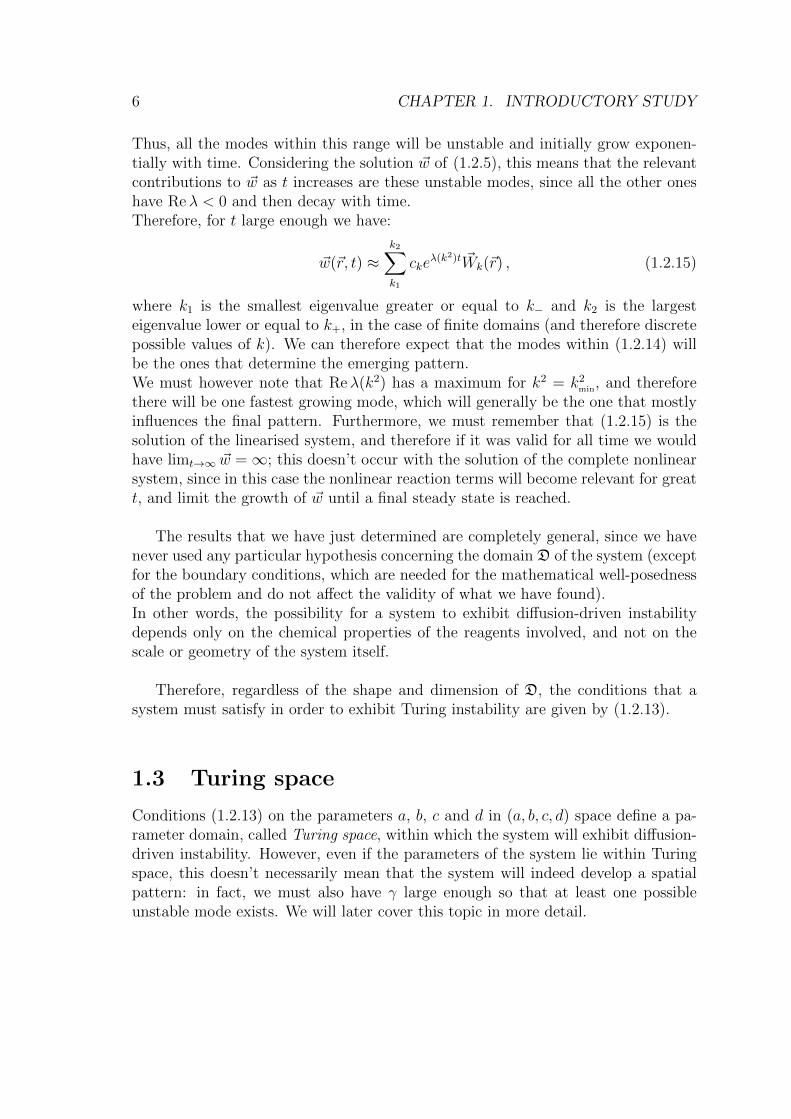
Thus, all the modes within this range will be unstable and initially grow exponen-tially with time. Considering the solution ~w of (1.2.5), this means that the relevantcontributions to ~w as t increases are these unstable modes, since all the other oneshave Reλ < 0 and then decay with time.Therefore, for t large enough we have:

~w(~r, t) ≈k2∑k1

ckeλ(k2)t ~Wk(~r) , (1.2.15)

where k1 is the smallest eigenvalue greater or equal to k− and k2 is the largesteigenvalue lower or equal to k+, in the case of finite domains (and therefore discretepossible values of k). We can therefore expect that the modes within (1.2.14) willbe the ones that determine the emerging pattern.We must however note that Reλ(k2) has a maximum for k2 = k2min, and thereforethere will be one fastest growing mode, which will generally be the one that mostlyinfluences the final pattern. Furthermore, we must remember that (1.2.15) is thesolution of the linearised system, and therefore if it was valid for all time we wouldhave limt→∞ ~w =∞; this doesn’t occur with the solution of the complete nonlinearsystem, since in this case the nonlinear reaction terms will become relevant for greatt, and limit the growth of ~w until a final steady state is reached.

The results that we have just determined are completely general, since we havenever used any particular hypothesis concerning the domain D of the system (exceptfor the boundary conditions, which are needed for the mathematical well-posednessof the problem and do not affect the validity of what we have found).In other words, the possibility for a system to exhibit diffusion-driven instabilitydepends only on the chemical properties of the reagents involved, and not on thescale or geometry of the system itself.

Therefore, regardless of the shape and dimension of D, the conditions that asystem must satisfy in order to exhibit Turing instability are given by (1.2.13).

1.3 Turing space

Conditions (1.2.13) on the parameters a, b, c and d in (a, b, c, d) space define a pa-rameter domain, called Turing space, within which the system will exhibit diffusion-driven instability. However, even if the parameters of the system lie within Turingspace, this doesn’t necessarily mean that the system will indeed develop a spatialpattern: in fact, we must also have γ large enough so that at least one possibleunstable mode exists. We will later cover this topic in more detail.

1.3. TURING SPACE 7

1.3.1 Determination of Turing space

The domain defined by inequalities (1.2.13) is not straightforward to represent (alsobecause it lives in a four-dimensional space); we are therefore going to introducesome simplifications in order to make the problem easier to study, and then gener-alise as much as we can.Let us then consider c and d fixed, so that we can first determine two-dimensionalsections of Turing space in (a, b) space.

In order to determine an explicit representation of this domain we use Murray’smethod (see [5]), i.e. we set u0 as a non-negative parametric variable and expressv0 and b in terms of u0 and a. We thus have:

v0 = u20 , b =a+ c

u0

and:

fu =c− au0

, fv = − c

u20, gu = 2u0 , gv = −1 .

We now express the conditions for Turing instability in terms of u0, so that we candetermine regions of (a, b) plane enclosed by parametric curves.The Turing space of the system will then be given by the intersection of these regions.

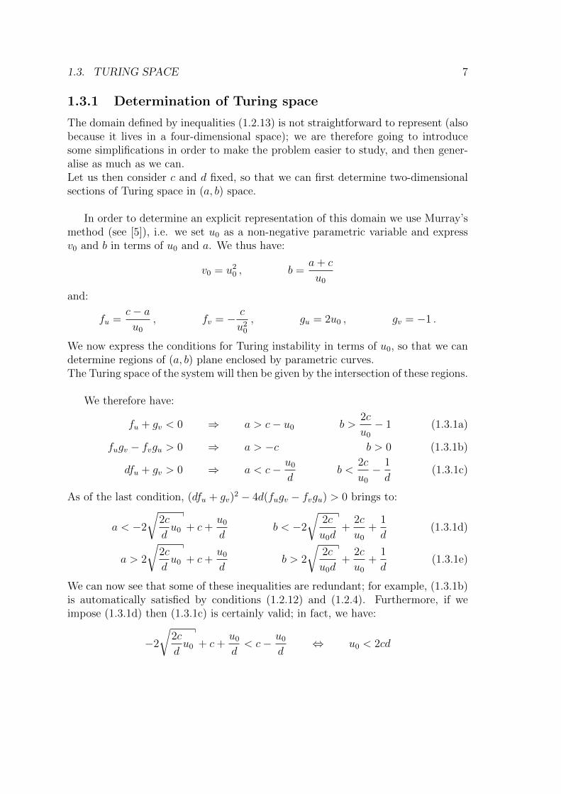
We therefore have:

fu + gv < 0 ⇒ a > c− u0 b >2c

u0− 1 (1.3.1a)

fugv − fvgu > 0 ⇒ a > −c b > 0 (1.3.1b)

dfu + gv > 0 ⇒ a < c− u0d

b <2c

u0− 1

d(1.3.1c)

As of the last condition, (dfu + gv)2 − 4d(fugv − fvgu) > 0 brings to:

a < −2

√2c

du0 + c+

u0d

b < −2

√2c

u0d+

2c

u0+

1

d(1.3.1d)

a > 2

√2c

du0 + c+

u0d

b > 2

√2c

u0d+

2c

u0+

1

d(1.3.1e)

We can now see that some of these inequalities are redundant; for example, (1.3.1b)is automatically satisfied by conditions (1.2.12) and (1.2.4). Furthermore, if weimpose (1.3.1d) then (1.3.1c) is certainly valid; in fact, we have:

−2

√2c

du0 + c+

u0d< c− u0

d⇔ u0 < 2cd


b

a(1.3.1a)

(1.3.1b) (1.3.1c)

(1.3.1d)

(1.3.1e)

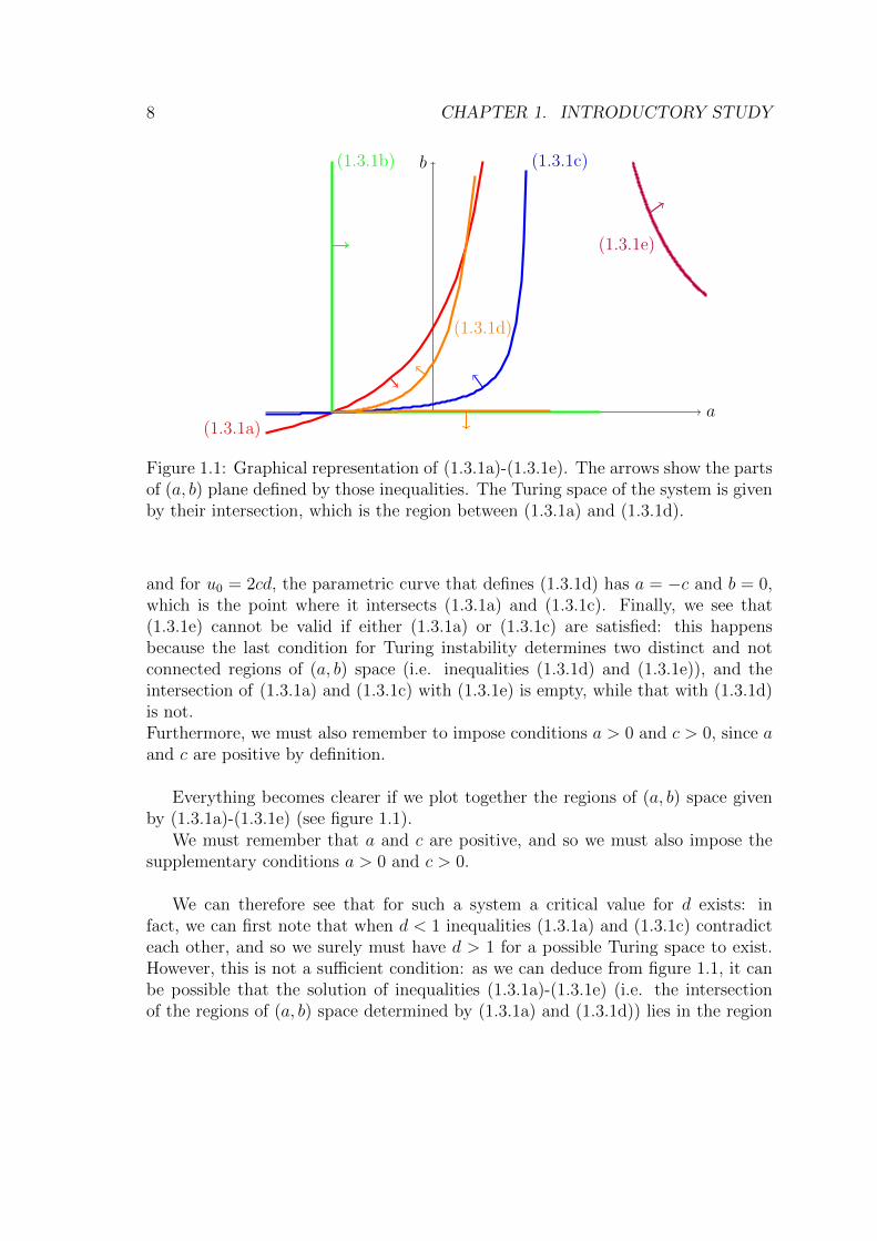
Figure 1.1: Graphical representation of (1.3.1a)-(1.3.1e). The arrows show the partsof (a, b) plane defined by those inequalities. The Turing space of the system is givenby their intersection, which is the region between (1.3.1a) and (1.3.1d).

and for u0 = 2cd, the parametric curve that defines (1.3.1d) has a = −c and b = 0,which is the point where it intersects (1.3.1a) and (1.3.1c). Finally, we see that(1.3.1e) cannot be valid if either (1.3.1a) or (1.3.1c) are satisfied: this happensbecause the last condition for Turing instability determines two distinct and notconnected regions of (a, b) space (i.e. inequalities (1.3.1d) and (1.3.1e)), and theintersection of (1.3.1a) and (1.3.1c) with (1.3.1e) is empty, while that with (1.3.1d)is not.Furthermore, we must also remember to impose conditions a > 0 and c > 0, since aand c are positive by definition.

Everything becomes clearer if we plot together the regions of (a, b) space givenby (1.3.1a)-(1.3.1e) (see figure 1.1).

We must remember that a and c are positive, and so we must also impose thesupplementary conditions a > 0 and c > 0.

We can therefore see that for such a system a critical value for d exists: infact, we can first note that when d < 1 inequalities (1.3.1a) and (1.3.1c) contradicteach other, and so we surely must have d > 1 for a possible Turing space to exist.However, this is not a sufficient condition: as we can deduce from figure 1.1, it canbe possible that the solution of inequalities (1.3.1a)-(1.3.1e) (i.e. the intersectionof the regions of (a, b) space determined by (1.3.1a) and (1.3.1d)) lies in the region

1.3. TURING SPACE 9

a < 0, and so in these conditions no actual Turing space exists.Therefore, in order to find the critical value dc for d we determine the intersectionof the parametric curves (1.3.1a) and (1.3.1d), setting:

c− u0 = −2

√2c

du0 + c+

u0d

⇒ u0 = 8cd

(d+ 1)2.

Thus, the value of a where (1.3.1a) and (1.3.1d) intersect each other is:

a = c− u0 = c

[1− 8

d

(d+ 1)2

].

By setting a > 0, we get:d2 − 6d+ 1 > 0 ,

whose solution is d < 3−2√

2 or d > 3+2√

2 . However, since d must be greater than1, for what stated previously, the only valid solution of the inequality is d > 3+2

√2 .

Therefore, dc = 3 + 2√

2 and if d < dc (with all the other parameters kept fixed) noTuring space exists.

1.3.2 Representation of Turing space

Therefore, Turing space for Gierer and Menihardt’s system is, for c and d fixed, theregion of (a, b) space enclosed between the two parametric curves:

(1.3.1a) :

{a = c− u0b = 2c

u0− 1

(1.3.1d) :

a = −2√

2cdu0 + c+ u0

d

b = −2√

2cu0d

+ 2cu0

+ 1d

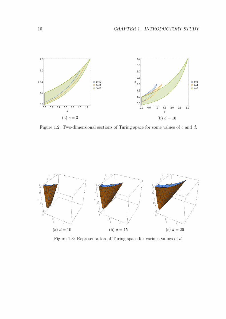
with a, c > 0.Figure 1.2 represents some examples of two-dimensional sections of Turing space forvarious values of fixed c and d, while in figure 1.3 Turing space is represented in(a, b, c) space, for d fixed.

1.3.3 Notes on Turing space

We can now deduce some general properties of Gierer and Meinhardt’s system.

From figure 1.3, we can see that it is not very robust : since its Turing spaceis quite “narrow”, reaction-diffusion systems obeying Gierer and Meinhardt’s equa-tions can be very sensible to random perturbations, which are always present inbiological contexts.


(a) c = 3 (b) d = 10

Figure 1.2: Two-dimensional sections of Turing space for some values of c and d.

(a) d = 10 (b) d = 15 (c) d = 20

Figure 1.3: Representation of Turing space for various values of d.

1.3. TURING SPACE 11

We can also note that diffusion-driven instability is the result of a combinationof various effects: if we suppose the system to be initially outside Turing space, thenthere will be several ways by which we can make it diffusively unstable; in fact, byvarying one or more of the parameters of the system we can “move” it inside Turingspace, and there is no single way to do it. Therefore, there will be different andequivalent effects, through the variation of the parameters of the system, that willlead to the formation of the same patterns.

Chapter 2

Gierer and Meinhardt’s system ona sphere

We will now proceed to the main part of this work, namely the study of Giererand Meinhardt’s system defined on a sphere of radius R, in order to investigate theeffects of curvature on pattern formation.

2.1 Initial considerations

The mathematical formulation of the problem we want to analyse is the following:

∂u

∂t= γ

(a− bu+ c

u2

v

)+∇2u

∂v

∂t= γ(u2 − v) + d∇2v

u(θ, ϕ, 0) and v(θ, ϕ, 0) given,

where we have written u and v in spherical coordinates, since D is now a sphere of(fixed) radius R, and curvature ρ = 1/R. Since the problem is defined on a sphere,no boundary conditions are required.

Note that γ is related to the curvature of the sphere, namely its size. By takingR as a characteristic length of the system we have γ = R2k5/DA = (1/ρ2)(k5/DA).We therefore must keep in mind that γ ∝ R2 = 1/ρ2, since this will be importantto determine the effects of curvature on spatial pattern formation on a sphere. Forfuture convenience, we set γ = Γ/ρ2 (namely, Γ = k5/DA).

The eigenvalue problem we have to solve now is:

∇2 ~Wk + k2 ~Wk = 0 ~Wk defined on D ,

13

14 CHAPTER 2. GIERER AND MEINHARDT’S SYSTEM ON A SPHERE

whose solutions are the spherical harmonics Y m` (θ, ϕ). Therefore we have:

k2 =`(`+ 1)

R2= ρ2`(`+ 1) (2.1.1)

(where ` = 0, 1, 2, . . . ) and we look for solutions of the complete linearised systemin the form:

~w(θ, ϕ, t) =∞∑`=0

∑m=−`

~Cm` e

λtY m` (θ, ϕ) , (2.1.2)

where ~Cm` are constants determined with an expansion of the initial conditions in

terms of spherical harmonics.

We can now apply all the results we have determined in 1.2 with the substitution(2.1.1), which is the particular form of the eigenvalues of the Laplacian in this case.We thus have:

k2min = ρ2`min(`min + 1) =Γ

2dρ2,

where we have set, for the sake of convenience, Γ = Γ(db c−a

c+a− 1). Therefore:

`2min + `min −Γ

2dρ4= 0 ⇒ `min = −1

2+

1

2

√1 +

2Γ

dρ4

and:

h(`min) =1

ρ4

(Γ2b− Γ2

4d

). (2.1.3)

The range of unstable modes is then given by:

`− < ` < `+ , `± = −1

2+

1

2

√1 +

2

dρ4

(Γ±

√Γ2 − 4dbΓ2

). (2.1.4)

Of course, this could also be determined by explicitly substitute (2.1.2) in system(1.2.5). In fact, by proceeding like in section 1.2.3 we find:

λ2 + λ

[ρ2`(`+ 1)(1 + d)− Γ

ρ2

(bc− ac+ a

− 1

)]+ h(`) = 0 , (2.1.5)

h(`) = dρ4`4 + 2dρ4`3 + (dρ4 − Γ)`2 − Γ`+Γ2

ρ4b . (2.1.6)

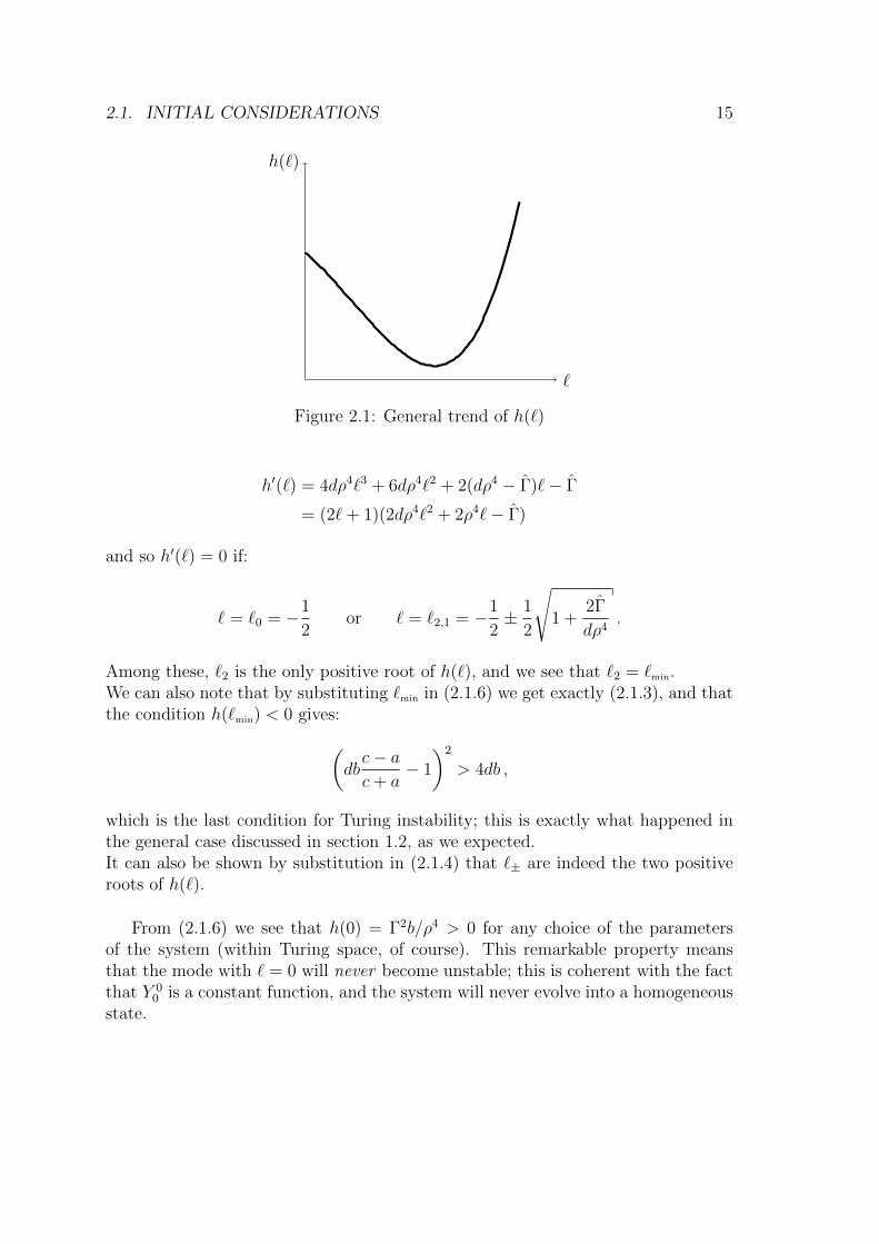
The behaviour of h(`) is reported in figure 2.1. Note that h(`) has only one minimumfor ` > 0. In fact:

2.1. INITIAL CONSIDERATIONS 15

h(`)

`

Figure 2.1: General trend of h(`)

h′(`) = 4dρ4`3 + 6dρ4`2 + 2(dρ4 − Γ)`− Γ

= (2`+ 1)(2dρ4`2 + 2ρ4`− Γ)

and so h′(`) = 0 if:

` = `0 = −1

2or ` = `2,1 = −1

2± 1

2

√1 +

2Γ

dρ4.

Among these, `2 is the only positive root of h(`), and we see that `2 = `min.We can also note that by substituting `min in (2.1.6) we get exactly (2.1.3), and thatthe condition h(`min) < 0 gives:(

dbc− ac+ a

− 1

)2

> 4db ,

which is the last condition for Turing instability; this is exactly what happened inthe general case discussed in section 1.2, as we expected.It can also be shown by substitution in (2.1.4) that `± are indeed the two positiveroots of h(`).

From (2.1.6) we see that h(0) = Γ2b/ρ4 > 0 for any choice of the parametersof the system (within Turing space, of course). This remarkable property meansthat the mode with ` = 0 will never become unstable; this is coherent with the factthat Y 0

0 is a constant function, and the system will never evolve into a homogeneousstate.


2.2 The role of curvature

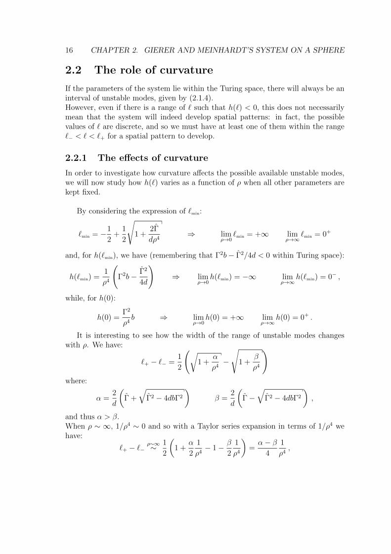
If the parameters of the system lie within the Turing space, there will always be aninterval of unstable modes, given by (2.1.4).However, even if there is a range of ` such that h(`) < 0, this does not necessarilymean that the system will indeed develop spatial patterns: in fact, the possiblevalues of ` are discrete, and so we must have at least one of them within the range`− < ` < `+ for a spatial pattern to develop.

2.2.1 The effects of curvature

In order to investigate how curvature affects the possible available unstable modes,we will now study how h(`) varies as a function of ρ when all other parameters arekept fixed.

By considering the expression of `min:

`min = −1

2+

1

2

√1 +

2Γ

dρ4⇒ lim

ρ→0`min = +∞ lim

ρ→∞`min = 0+

and, for h(`min), we have (remembering that Γ2b− Γ2/4d < 0 within Turing space):

h(`min) =1

ρ4

(Γ2b− Γ2

4d

)⇒ lim

ρ→0h(`min) = −∞ lim

ρ→∞h(`min) = 0− ,

while, for h(0):

h(0) =Γ2

ρ4b ⇒ lim

ρ→0h(0) = +∞ lim

ρ→∞h(0) = 0+ .

It is interesting to see how the width of the range of unstable modes changeswith ρ. We have:

`+ − `− =1

2

(√1 +

α

ρ4−

√1 +

β

ρ4

)where:

α =2

d

(Γ +

√Γ2 − 4dbΓ2

)β =

2

d

(Γ−

√Γ2 − 4dbΓ2

),

and thus α > β.When ρ ∼ ∞, 1/ρ4 ∼ 0 and so with a Taylor series expansion in terms of 1/ρ4 wehave:

`+ − `−ρ∼∞∼ 1

2

(1 +

α

2

1

ρ4− 1− β

2

1

ρ4

)=α− β

4

1

ρ4,

2.2. THE ROLE OF CURVATURE 17

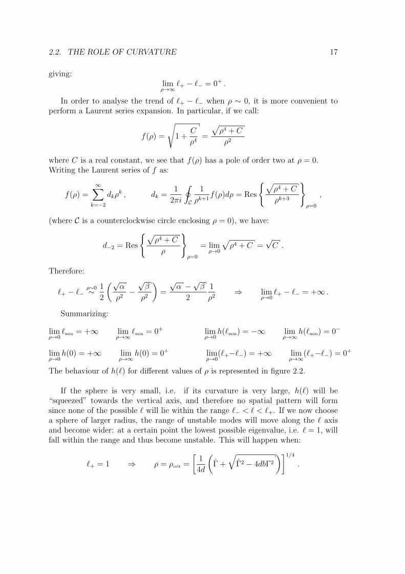
giving:limρ→∞

`+ − `− = 0+ .

In order to analyse the trend of `+ − `− when ρ ∼ 0, it is more convenient toperform a Laurent series expansion. In particular, if we call:

f(ρ) =

√1 +

C

ρ4=

√ρ4 + C

ρ2

where C is a real constant, we see that f(ρ) has a pole of order two at ρ = 0.Writing the Laurent series of f as:

f(ρ) =∞∑

k=−2

dkρk , dk =

1

2πi

∮C

1

ρk+1f(ρ)dρ = Res

{√ρ4 + C

ρk+3

}ρ=0

,

(where C is a counterclockwise circle enclosing ρ = 0), we have:

d−2 = Res

{√ρ4 + C

ρ

}ρ=0

= limρ→0

√ρ4 + C =

√C .

Therefore:

`+ − `−ρ∼0∼ 1

2

(√α

ρ2−√β

ρ2

)=

√α −

√β

2

1

ρ2⇒ lim

ρ→0`+ − `− = +∞ .

Summarizing:

limρ→0

`min = +∞ limρ→∞

`min = 0+ limρ→0

h(`min) = −∞ limρ→∞

h(`min) = 0−

limρ→0

h(0) = +∞ limρ→∞

h(0) = 0+ limρ→0

(`+−`−) = +∞ limρ→∞

(`+−`−) = 0+

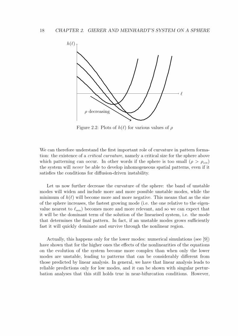
The behaviour of h(`) for different values of ρ is represented in figure 2.2.

If the sphere is very small, i.e. if its curvature is very large, h(`) will be“squeezed” towards the vertical axis, and therefore no spatial pattern will formsince none of the possible ` will lie within the range `− < ` < `+. If we now choosea sphere of larger radius, the range of unstable modes will move along the ` axisand become wider: at a certain point the lowest possible eigenvalue, i.e. ` = 1, willfall within the range and thus become unstable. This will happen when:

`+ = 1 ⇒ ρ = ρcrit =

[1

4d

(Γ +

√Γ2 − 4dbΓ2

)]1/4.


h(`)

`

ρ decreasing

Figure 2.2: Plots of h(`) for various values of ρ

We can therefore understand the first important role of curvature in pattern forma-tion: the existence of a critical curvature, namely a critical size for the sphere abovewhich patterning can occur. In other words if the sphere is too small (ρ > ρcrit)the system will never be able to develop inhomogeneous spatial patterns, even if itsatisfies the conditions for diffusion-driven instability.

Let us now further decrease the curvature of the sphere: the band of unstablemodes will widen and include more and more possible unstable modes, while theminimum of h(`) will become more and more negative. This means that as the sizeof the sphere increases, the fastest growing mode (i.e. the one relative to the eigen-value nearest to `min) becomes more and more relevant, and so we can expect thatit will be the dominant term of the solution of the linearised system, i.e. the modethat determines the final pattern. In fact, if an unstable modes grows sufficientlyfast it will quickly dominate and survive through the nonlinear region.

Actually, this happens only for the lower modes: numerical simulations (see [9])have shown that for the higher ones the effects of the nonlinearities of the equationson the evolution of the system become more complex than when only the lowermodes are unstable, leading to patterns that can be considerably different fromthose predicted by linear analysis. In general, we have that linear analysis leads toreliable predictions only for low modes, and it can be shown with singular pertur-bation analyses that this still holds true in near-bifurcation conditions. However,

2.3. THE ROLE OF INITIAL CONDITIONS 19

we must note that this method determines correctly parameter ranges for patternformation, namely Turing space.

Therefore, for big enough spheres the final steady state can be different fromwhat we can predict with the method we are using.

2.2.2 Mode selection

We would now like to answer a simple question: how can we excite a selected mode?In other words, by changing the radius of the sphere, how can we make sure that agiven mode will become unstable and hence determine the final pattern?We can use what we have previously stated so that the selected mode will have thelargest growth factor. If we call `chs the eigenvalue of the mode we have chosen toexcite, this will occur if `min = `chs, namely:

ρ =

{2Γ

d [(2`chs + 1)2 − 1]

}1/4

.

2.3 The role of initial conditions

Until now we have always neglected the effects that initial conditions might have onthe evolution of spatial patterns. As we shall now see, they are extremely importantand determine some relevant properties of the final pattern.

2.3.1 Polarity

We have seen in section 1.2.3 that in general if a system is diffusively unstable anda range of possible unstable modes exists, for t large enough the solution ~w of thecomplete linearised system of Gierer and Meinhardt’s equations is (1.2.5):

~w(~r, t) ≈k2∑k1

ckeλ(k2)t ~Wk(~r)

where k1 and k2 are, respectively, the smallest and largest possible eigenvalues withinthe range of unstable modes.In the case we are considering, i.e. when the domain D is a spherical surface, wehave:

~w(θ, ϕ, t) ≈`2∑`=`1

∑m=−`

~Cm` e

λ(`)tY m` (θ, ϕ) (2.3.1)


where `1 is the smallest eigenvalue greater or equal to `− and `2 is the largest onelower or equal to `+.Let us now suppose, for example, that the system is such that only the mode with` = 1 and m = 0 is unstable; we then have:

~w(θ, ϕ, t) ≈ ~C01eλ(1)tY 0

1 (θ, ϕ)

and ~C01 is a vector of constants determined, as usual, with an expansion of initial

conditions in terms of Y 01 .

To get a better understanding of how initial conditions can influence the polarity ofthe final pattern, let us suppose ~C0

1 to be (ε, ε) for ε > 0 small. Therefore:

~w(θ, ϕ, t) ≈(εε

)eλ(1)tY 0

1 (θ, ϕ)

and considering the single components of ~w:

u(θ, ϕ, t) ≈ u0 + εeλ(1)tY 01 (θ, ϕ) v(θ, ϕ, t) ≈ v0 + εeλ(1)tY 0

1 (θ, ϕ) .

We therefore have that both u and v will finally be spatially arranged like thespherical harmonic of order one, i.e. with u > u0 and v > v0 in one of the twohemispheres.However, if we now suppose to have ~C0

1 = (−ε, ε), then:

u(θ, ϕ, t) ≈ u0 − εeλ(1)tY 01 (θ, ϕ) v(θ, ϕ, t) ≈ v0 − εeλ(1)tY 0

1 (θ, ϕ)

which is the same arrangement of the preceding case, but with opposite polarity.Therefore, we can see that for any possible excited mode we have two possible dif-ferent patterns, each with opposite polarity, that are both solutions of the linearisedsystem of equations.This poses some conceptual difficulties under a biological point of view, within thecontext of prepattern theory: in fact, what we have just seen means that if cellsdifferentiate when the concentration of a morphogen exceeds some threshold level,then the differentiated cell pattern is different for each case. However, developmentis a sequential process, i.e. every stage of the development induces the next one;therefore this means that there must be a bias in the initial conditions towards one ofthe possible patterns. This is still an open issue, and is exactly what we have statedin the preface: we still don’t know the mechanism that links genetic informationand the bias on the initial conditions that leads to the final pattern.

2.3.2 Order of the unstable modes

Another fact that we have completely ignored until now is that in this case sphericalharmonics are degenerate with respect to the eigenvalue `. In fact, for a fixed value

2.4. CONCLUSIONS 21

of ` there are 2` + 1 different possible spherical harmonics, and we can only excitea certain value of `, i.e. the degree of the spherical harmonics. Therefore, if we usemode selection in order to excite a particular `, we still don’t know exactly whatwill the final heterogeneous pattern look like because we have no way to select anyof those 2` + 1 possible spherical harmonics by only varying the parameters of thesystem.In fact, if we suppose that the only unstable mode is that relative to the eigenvalue`, (2.3.1) becomes:

~w(θ, ϕ, t) ≈∑m=−`

~Cm` e

λ(`)tY m` (θ, ϕ)

and the order of the final pattern is determined by ~Cm` . For example, if we take

` = 3 and ~C23 = (ε, ε) for ε > 0 small, while ~Cm

3 = 0 for m 6= 2, we will have:

~w(θ, ϕ, t) ≈(εε

)eλ(3)tY 2

3 (θ, ϕ) .

Therefore, the conceptual difficulty we have described in the preceding sectionbecomes even more challenging if we consider that also the order of the excitedspherical harmonic depends on a bias on the initial conditions.

2.4 Conclusions

We have made a simple linear analysis of a system composed of two chemical reagentsobeying Gierer and Meinhardt’s equations on a spherical surface in order to deter-mine the spatial patterns that might develop from such a system. We have seenthat Turing instability occurs when conditions:

bc− ac+ a

< 1 , b > 0 , dbc− ac+ a

> 1 ,

(dbc− ac+ a

− 1

)2

> 4db

are satisfied, which confirms the predictions already known for flat surfaces. In thiscase, a range of unstable modes always exists and is given by:

`− < ` < `+ , `± = −1

2+

1

2

√1 +

2

dρ4

(Γ±

√Γ2 − 4dbΓ2

),

where Γ = k5/DA and Γ = Γ(db c−a

c+a− 1).

We have then seen how this range behaves as a function of the curvature ρ, and havededuced that a critical value for ρ exists, i.e. is the sphere is too small the system


will never be able to develop inhomogeneous spatial patterns, even if it satisfies theaforementioned conditions for diffusion-driven instability. We have also seen that asthe curvature decreases, the range of possible unstable modes becomes wider andthus more complex pattern can be generated as the radius of the sphere increases.Therefore, for a fixed value R = 1/ρ of the radius we can conclude that the set ofpatterns that can develop from the system are the spherical harmonics of degree `included in the aforementioned range. In particular the dominant pattern (i.e. theone with the largest growth factor) will be that with degree ` nearest to `min, where:

`min = −1

2+

1

2

√1 +

2Γ

dρ4.

We have also stated that linear prediction is reliable only near bifurcation condi-tions and for the lowest values of `, and must be used only as a guide to understandthe final pattern when higher modes are unstable.Finally, we have also seen that the order m of the unstable spherical harmonics, aswell as their polarity, are determined only by initial conditions.

2.5 Numerical simulations

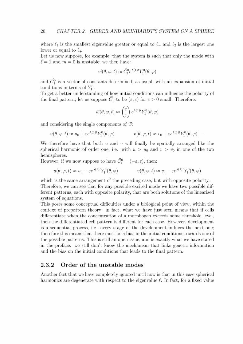
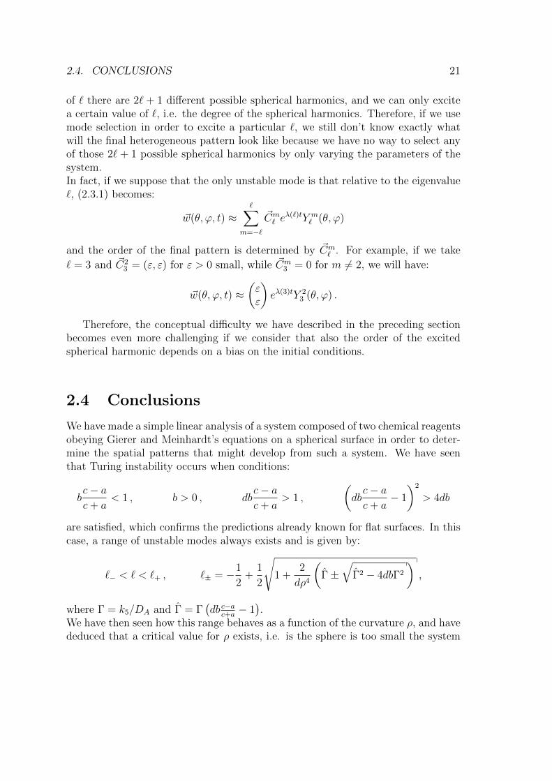
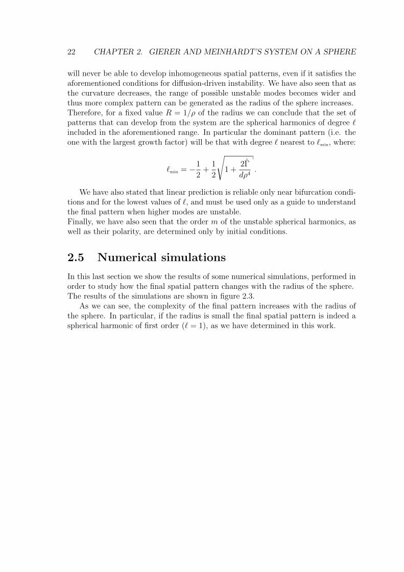
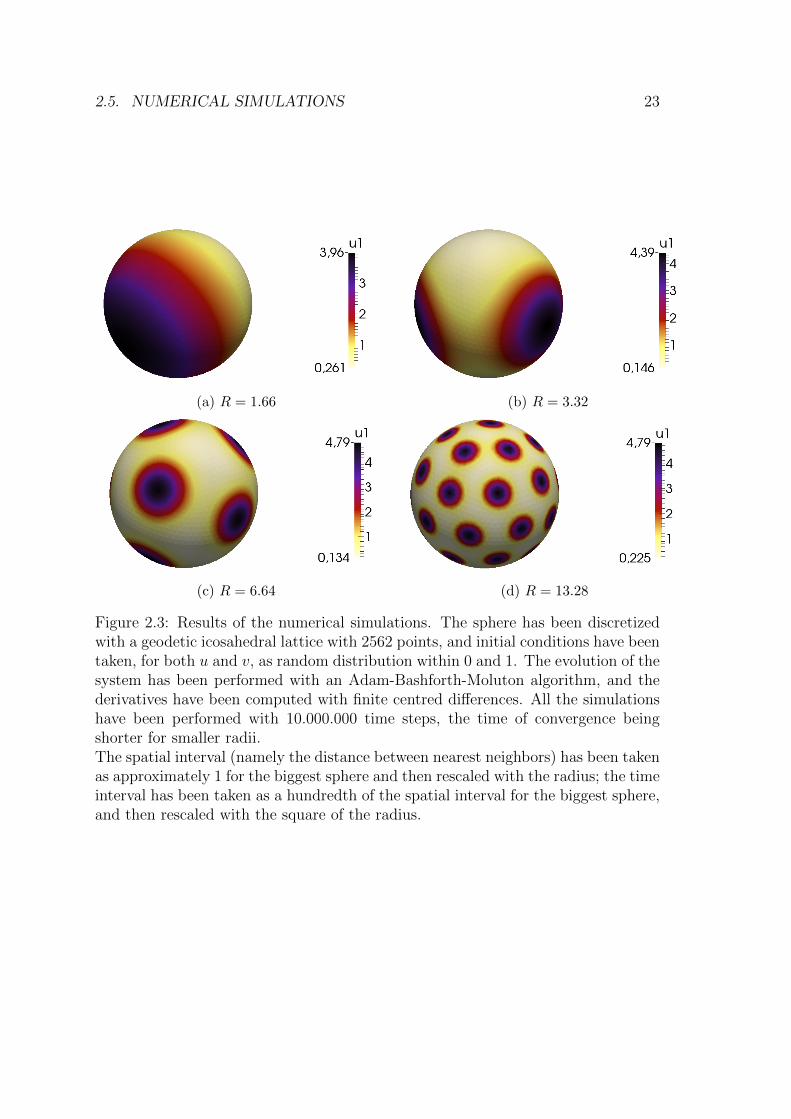
In this last section we show the results of some numerical simulations, performed inorder to study how the final spatial pattern changes with the radius of the sphere.The results of the simulations are shown in figure 2.3.

As we can see, the complexity of the final pattern increases with the radius ofthe sphere. In particular, if the radius is small the final spatial pattern is indeed aspherical harmonic of first order (` = 1), as we have determined in this work.

2.5. NUMERICAL SIMULATIONS 23

(a) R = 1.66 (b) R = 3.32

(c) R = 6.64 (d) R = 13.28

Figure 2.3: Results of the numerical simulations. The sphere has been discretizedwith a geodetic icosahedral lattice with 2562 points, and initial conditions have beentaken, for both u and v, as random distribution within 0 and 1. The evolution of thesystem has been performed with an Adam-Bashforth-Moluton algorithm, and thederivatives have been computed with finite centred differences. All the simulationshave been performed with 10.000.000 time steps, the time of convergence beingshorter for smaller radii.The spatial interval (namely the distance between nearest neighbors) has been takenas approximately 1 for the biggest sphere and then rescaled with the radius; the timeinterval has been taken as a hundredth of the spatial interval for the biggest sphere,and then rescaled with the square of the radius.

Bibliography

[1] J. D. Murray, Mathematical Biology (third edition), Volume 2, Springer-Verlag,2003

[2] A. M. Turing, The chemical basis of morphogenesis, Philosophical Transactionsof the Royal Society of London, series B, 237:37–72, 1952

[3] T. Laux et al., Genetic regulation of embryonic pattern formation, The PlantCell, 2004

[4] A. Gierer and H. Meinhardt, A theory of biological pattern formation, Kyber-netik, 12:30–39, 1972

[5] J. D. Murray, Parameter space for Turing instability in reaction diffusion mech-anisms: a comparison of models, Journal of Theoretical Biology, 98:143–163,1982

[6] A.J. Koch and H. Meinhardt, Biological pattern formation: from basic mecha-nisms to complex structures, Review of Modern Physics, 66:1481–1507, 1994

[7] L. Wolpert, Positional information and the spatial pattern of cellular differenti-ation, Journal of Theoretical Biology, 25:1–47, 1969

[8] G. F. Oster and J. D. Murray, Pattern formation models and developmentalconstraints, The Journal of Experimental Zoology, 251:186–202, 1989

[9] P. Arcuri and J. D. Murray, Pattern sensitivity to boundary and initial conditionsin reaction-diffusion models, Journal of Mathematical Biology, 24:141–165, 1986

25

curvature effect on patterning dynamics on spherical...

Documents