current limitations of sequential inference in general hidden markov models
TRANSCRIPT
Current limitations of sequential inference ingeneral hidden Markov models
Pierre JacobDepartment of Statistics, University of Oxford
March 5th
Pierre Jacob Sequential inference in HMM 1/ 60
Outline
1 Setting: online inference in time seriesHidden Markov ModelsImplicit modelsExact / sequential / online methods
2 Plug and play methodsApproximate Bayesian ComputationParticle Filters
3 SMC2 for sequential inferenceA sequential method for HMMNot online
4 Numerical experiments
5 Discussion
Pierre Jacob Sequential inference in HMM 2/ 60
Hidden Markov Models
y2y1 yT
X2X0 X1 XT
y0
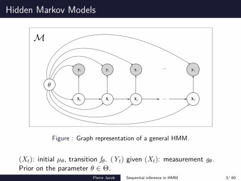
Figure : Graph representation of a general HMM.
(Xt): initial µθ, transition fθ. (Yt) given (Xt): measurement gθ.Prior on the parameter θ ∈ Θ.
Pierre Jacob Sequential inference in HMM 3/ 60
Phytoplankton–Zooplankton
●●●
●
●●
●
●●●●●
●●
●
●●
●
●
●
●
●
●●●●
●
●
●
●
●●
●
●●
●●
●●
●
●
●
●
●
●
●●●●
●
●
●
●
●
●
●●●●●
●
●
●
●
●
●
●●●
●
●
●
●
●
●●●●●●
●
●
●
●●●
●
●●
●●
●
●
●●
●
●
●●
●●
●
●
●●●●
●
●●
●
●
●
●●●●●
●
●
●
●
●
●●●●
●●●●
●●
●
●
●
●
●
●
●●
●
●●
●
●
●
●●●●
●●
●
●
●
●
●●
●
●●●
●
●
●
●●●●●●
●
●●
●
●
●
●
●
●
●
●●
●
●
●
●
●●●●●●●●
●●
●
●
●
●
●●
●●●
●
●
●
●
●●●
●
●
●
●
●●●●●
●●●●
●
●
●
●
●●●
●●●
●●
●
●
●
●
●
●●
●
●●
●●●●
●●
●
●●●●●●
●
●
●●
●●
●
●●
●
●
●
●
●
●
●
●
●
●
●
●
●●●●
●
●
●
●●
●
●
●
●
●
●
●
●
●
●
●
●●
●
●●
●
●
●
●
●
●
●
●
●●●
●
●
●
●●●●
●●●
●
●
●
●
●
●
●
●●
●●
●
●
●
●
●
●●
●●●●●●
●●
●
●
●
●
●
●●●●
●
●
0
10
20
30
40
0 100 200 300time
obse
rvat
ions
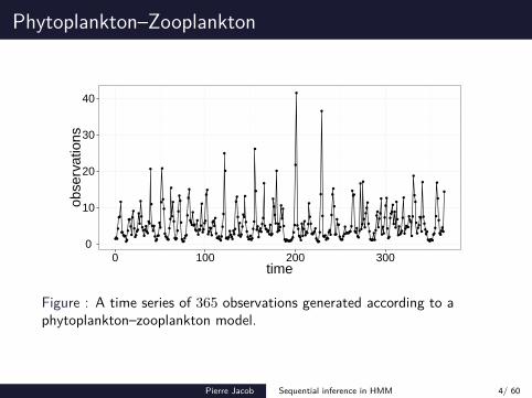
Figure : A time series of 365 observations generated according to aphytoplankton–zooplankton model.
Pierre Jacob Sequential inference in HMM 4/ 60
General questions
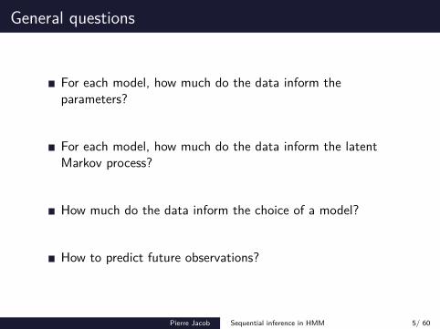
For each model, how much do the data inform theparameters?
For each model, how much do the data inform the latentMarkov process?
How much do the data inform the choice of a model?
How to predict future observations?
Pierre Jacob Sequential inference in HMM 5/ 60
Questions translated into integrals
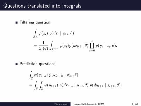
Filtering question:∫Xφ(xt) p(dxt | y0:t , θ)
= 1Zt(θ)
∫Xt+1
φ(xt)p(dx0:t | θ)t∏
s=0p(ys | xs, θ).
Prediction question:∫Yφ(yt+k) p(dyt+k | y0:t , θ)
=∫Y
∫Xφ(yt+k) p(dxt+k | y0:t , θ) p(dyt+k | xt+k , θ).
Pierre Jacob Sequential inference in HMM 6/ 60
Questions translated into integrals
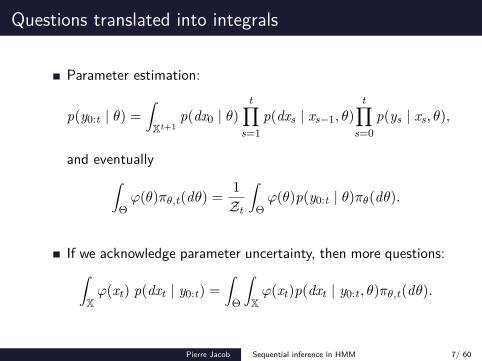
Parameter estimation:
p(y0:t | θ) =∫Xt+1
p(dx0 | θ)t∏
s=1p(dxs | xs−1, θ)
t∏s=0
p(ys | xs, θ),
and eventually∫Θφ(θ)πθ,t(dθ) = 1
Zt
∫Θφ(θ)p(y0:t | θ)πθ(dθ).
If we acknowledge parameter uncertainty, then more questions:∫Xφ(xt) p(dxt | y0:t) =
∫Θ
∫Xφ(xt)p(dxt | y0:t , θ)πθ,t(dθ).
Pierre Jacob Sequential inference in HMM 7/ 60
Questions translated into integrals
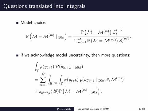
Model choice:
P(M =M(m) | y0:t
)=
P(M =M(m)
)Z(m)
t∑Mm′=1 P
(M =M(m′))Z(m′)
t.
If we acknowledge model uncertainty, then more questions:∫Yφ(yt+k) P(dyt+k | y0:t)
=M∑
m=1
∫Θ(m)
∫Yφ(yt+k) p(dyt+k | y0:t , θ,M(m))
× πθ(m),t(dθ)P(M =M(m) | y0:t
).
Pierre Jacob Sequential inference in HMM 8/ 60
Outline
1 Setting: online inference in time seriesHidden Markov ModelsImplicit modelsExact / sequential / online methods
2 Plug and play methodsApproximate Bayesian ComputationParticle Filters
3 SMC2 for sequential inferenceA sequential method for HMMNot online
4 Numerical experiments
5 Discussion
Pierre Jacob Sequential inference in HMM 8/ 60
Phytoplankton–Zooplankton model
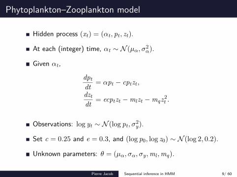
Hidden process (xt) = (αt , pt , zt).
At each (integer) time, αt ∼ N (µα, σ2α).
Given αt ,
dptdt
= αpt − cptzt ,
dztdt
= ecptzt −mlzt −mqz2t .
Observations: log yt ∼ N (log pt , σ2y).
Set c = 0.25 and e = 0.3, and (log p0, log z0) ∼ N (log 2, 0.2).
Unknown parameters: θ = (µα, σα, σy,ml ,mq).
Pierre Jacob Sequential inference in HMM 9/ 60

Implicit models
Even simple, standard scientific models are such that theimplied probability distribution p(dx0:t | θ) admits a densityfunction that cannot be computed pointwise.
To cover as many models as possible, we can only assumethat the hidden process can be simulated.
This covers cases where xt = ψ(xt−1, k, v1:k), for some integerk, vector v1:k ∈ Rk , and deterministic function ψ.
Calls for “plug and play” methods.
Time series analysis via mechanistic models,Breto, He, Ionides and King, 2009.
Pierre Jacob Sequential inference in HMM 10/ 60
Outline
1 Setting: online inference in time seriesHidden Markov ModelsImplicit modelsExact / sequential / online methods
2 Plug and play methodsApproximate Bayesian ComputationParticle Filters
3 SMC2 for sequential inferenceA sequential method for HMMNot online
4 Numerical experiments
5 Discussion
Pierre Jacob Sequential inference in HMM 10/ 60
Exact methods
Consider the problem of estimating some quantity It .
Consider an estimator I Nt where N is a tuning parameter.
Hopefully N is such that I Nt
some sense−−−−−−→N→∞
It .
For instance E[(I Nt − It)2] goes to zero when N →∞.
Variational methods / Ensemble Kalman Filters are not exact.
Consider the estimator that always returns 29.5. . .
Pierre Jacob Sequential inference in HMM 11/ 60
Sequential methods
Consider the problem of estimating some quantity It , for allt ≥ 0, e.g. upon the arrival of new data.
Assume the quantities It for all t ≥ 0 are related one to theother.
A sequential method “updates” the estimate I Nt into I N
t+1.
MCMC methods are not sequential: they have to be re-runfrom scratch whenever a new observation arrives.
Therefore, sequential methods are not to be confused withiterative methods.
Pierre Jacob Sequential inference in HMM 12/ 60
Online methods
Consider the problem of estimating some quantity It , for allt ≥ 0, e.g. upon the arrival of new data.
A method is online if it provides estimates I Nt of It for all
t ≥ 0, such that. . .
. . . the computational cost of obtaining each I Nt given I N
t−1 isindependent of t,
. . . the precision of the estimate does not explode over time:
r(I Nt ) =
(E
[(I N
t − It)2])1/2
|It |
can be uniformly bounded over t.
Consider the estimator that always returns 29.5. . .
Pierre Jacob Sequential inference in HMM 13/ 60
Outline
1 Setting: online inference in time seriesHidden Markov ModelsImplicit modelsExact / sequential / online methods
2 Plug and play methodsApproximate Bayesian ComputationParticle Filters
3 SMC2 for sequential inferenceA sequential method for HMMNot online
4 Numerical experiments
5 Discussion
Pierre Jacob Sequential inference in HMM 13/ 60
Approximate Bayesian Computation
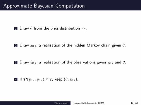
1 Draw θ from the prior distribution πθ.
2 Draw x0:t , a realisation of the hidden Markov chain given θ.
3 Draw y0:t , a realisation of the observations given x0:t and θ.
4 If D(y0:t , y0:t) ≤ ε, keep (θ, x0:t).
Pierre Jacob Sequential inference in HMM 14/ 60
Approximate Bayesian Computation
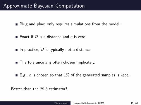
Plug and play: only requires simulations from the model.
Exact if D is a distance and ε is zero.
In practice, D is typically not a distance.
The tolerance ε is often chosen implicitely.
E.g., ε is chosen so that 1% of the generated samples is kept.
Better than the 29.5 estimator?
Pierre Jacob Sequential inference in HMM 15/ 60
Outline
1 Setting: online inference in time seriesHidden Markov ModelsImplicit modelsExact / sequential / online methods
2 Plug and play methodsApproximate Bayesian ComputationParticle Filters
3 SMC2 for sequential inferenceA sequential method for HMMNot online
4 Numerical experiments
5 Discussion
Pierre Jacob Sequential inference in HMM 15/ 60
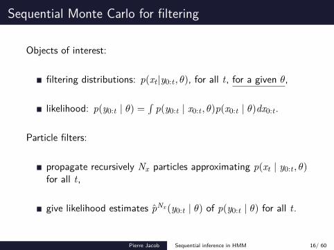
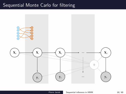
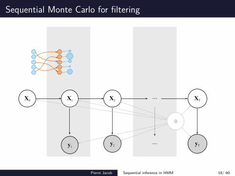
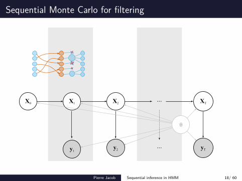
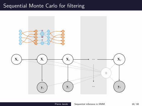
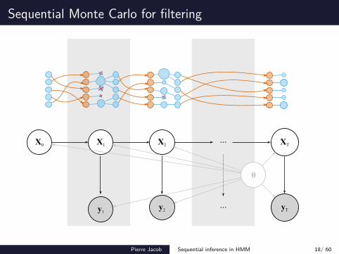
Sequential Monte Carlo for filtering
Objects of interest:
filtering distributions: p(xt |y0:t , θ), for all t, for a given θ,
likelihood: p(y0:t | θ) =∫
p(y0:t | x0:t , θ)p(x0:t | θ)dx0:t .
Particle filters:
propagate recursively Nx particles approximating p(xt | y0:t , θ)for all t,
give likelihood estimates pNx (y0:t | θ) of p(y0:t | θ) for all t.
Pierre Jacob Sequential inference in HMM 16/ 60
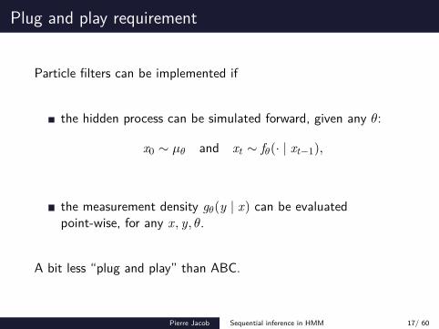
Plug and play requirement
Particle filters can be implemented if
the hidden process can be simulated forward, given any θ:
x0 ∼ µθ and xt ∼ fθ(· | xt−1),
the measurement density gθ(y | x) can be evaluatedpoint-wise, for any x, y, θ.
A bit less “plug and play” than ABC.
Pierre Jacob Sequential inference in HMM 17/ 60

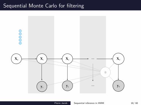
Sequential Monte Carlo for filtering
y2
X2X0
y1
X1...
... yT
XT
θ
Pierre Jacob Sequential inference in HMM 18/ 60
Sequential Monte Carlo for filtering
y2
X2X0
y1
X1...
... yT
XT
θ
Pierre Jacob Sequential inference in HMM 18/ 60
Sequential Monte Carlo for filtering
y2
X2X0
y1
X1...
... yT
XT
θ
Pierre Jacob Sequential inference in HMM 18/ 60
Sequential Monte Carlo for filtering
y2
X2X0
y1
X1...
... yT
XT
θ
Pierre Jacob Sequential inference in HMM 18/ 60
Sequential Monte Carlo for filtering
y2
X2X0
y1
X1...
... yT
XT
θ
Pierre Jacob Sequential inference in HMM 18/ 60
Sequential Monte Carlo for filtering
y2
X2X0
y1
X1...
... yT
XT
θ
Pierre Jacob Sequential inference in HMM 18/ 60
Sequential Monte Carlo for filtering
y2
X2X0
y1
X1...
... yT
XT
θ
Pierre Jacob Sequential inference in HMM 18/ 60

Sequential Monte Carlo for filtering
Consider I (φt) =∫φt(xt)p(xt | y0:t)dxt .
Lp-bound:
E[∣∣∣I N (φt)− I (φt)
∣∣∣p]1/p≤ c(p) ||φt ||∞√
N.
Central limit theorem:√
N(I N (φt)− I (φt)
) D−−−−→N→∞
N(0, σ2
t
).
where σ2t < σ2
max for all t.
Particle filters are fully online, plug and play, and exact. . . forfiltering.
Pierre Jacob Sequential inference in HMM 19/ 60
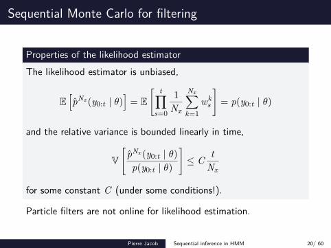
Sequential Monte Carlo for filtering
Properties of the likelihood estimatorThe likelihood estimator is unbiased,
E[pNx (y0:t | θ)
]= E
[ t∏s=0
1Nx
Nx∑k=1
wks
]= p(y0:t | θ)
and the relative variance is bounded linearly in time,
V[
pNx (y0:t | θ)p(y0:t | θ)
]≤ C t
Nx
for some constant C (under some conditions!).
Particle filters are not online for likelihood estimation.
Pierre Jacob Sequential inference in HMM 20/ 60
Outline
1 Setting: online inference in time seriesHidden Markov ModelsImplicit modelsExact / sequential / online methods
2 Plug and play methodsApproximate Bayesian ComputationParticle Filters
3 SMC2 for sequential inferenceA sequential method for HMMNot online
4 Numerical experiments
5 Discussion
Pierre Jacob Sequential inference in HMM 20/ 60
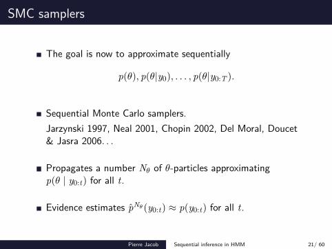
SMC samplers
The goal is now to approximate sequentially
p(θ), p(θ|y0), . . . , p(θ|y0:T ).
Sequential Monte Carlo samplers.Jarzynski 1997, Neal 2001, Chopin 2002, Del Moral, Doucet& Jasra 2006. . .
Propagates a number Nθ of θ-particles approximatingp(θ | y0:t) for all t.
Evidence estimates pNθ (y0:t) ≈ p(y0:t) for all t.
Pierre Jacob Sequential inference in HMM 21/ 60
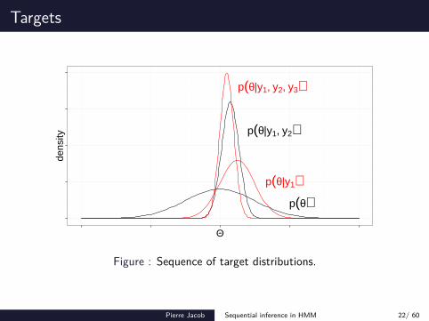
Targets
p(θ|y1)
p(θ|y1, y2)
p(θ|y1, y2, y3)
p(θ)
Θ
dens
ity
Figure : Sequence of target distributions.
Pierre Jacob Sequential inference in HMM 22/ 60
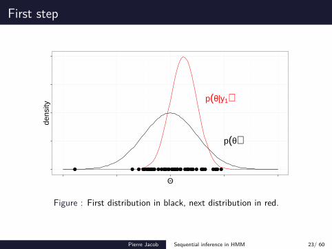
First step
p(θ|y1)
p(θ)
● ●●● ●● ● ●●● ●● ●● ●● ●● ●●●●● ●● ●●●●●● ●●● ● ●●● ●● ●●● ● ●● ●● ●●
Θ
dens
ity
Figure : First distribution in black, next distribution in red.
Pierre Jacob Sequential inference in HMM 23/ 60
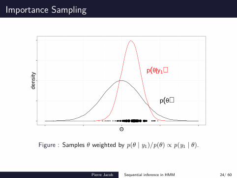
Importance Sampling
p(θ|y1)
p(θ)
● ●●● ●● ● ●●● ●● ●● ●● ●● ●●●●● ●● ●● ●●●● ● ●● ● ●●● ●● ●● ● ● ●● ●● ●●
Θ
dens
ity
Figure : Samples θ weighted by p(θ | y1)/p(θ) ∝ p(y1 | θ).
Pierre Jacob Sequential inference in HMM 24/ 60
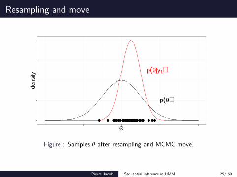
Resampling and move
p(θ|y1)
p(θ)
● ●●●● ●● ● ● ●●● ●● ●●● ●●● ●●●● ●●● ●● ●● ● ●●● ● ●●● ● ●● ●●● ●● ● ●●
Θ
dens
ity
Figure : Samples θ after resampling and MCMC move.
Pierre Jacob Sequential inference in HMM 25/ 60
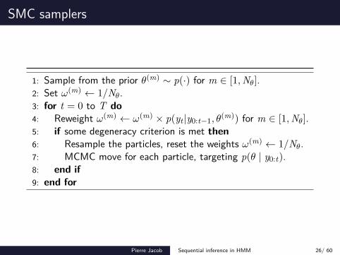
SMC samplers
1: Sample from the prior θ(m) ∼ p(·) for m ∈ [1,Nθ].2: Set ω(m) ← 1/Nθ.3: for t = 0 to T do4: Reweight ω(m) ← ω(m) × p(yt |y0:t−1, θ
(m)) for m ∈ [1,Nθ].5: if some degeneracy criterion is met then6: Resample the particles, reset the weights ω(m) ← 1/Nθ.7: MCMC move for each particle, targeting p(θ | y0:t).8: end if9: end for
Pierre Jacob Sequential inference in HMM 26/ 60
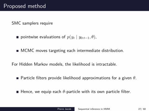
Proposed method
SMC samplers require
pointwise evaluations of p(yt | y0:t−1, θ),
MCMC moves targeting each intermediate distribution.
For Hidden Markov models, the likelihood is intractable.
Particle filters provide likelihood approximations for a given θ.
Hence, we equip each θ-particle with its own particle filter.
Pierre Jacob Sequential inference in HMM 27/ 60
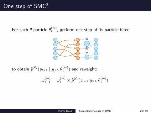
One step of SMC2
For each θ-particle θ(m)t , perform one step of its particle filter:
to obtain pNx (yt+1 | y0:t , θ(m)t ) and reweight:
ω(m)t+1 = ω
(m)t × pNx (yt+1|y0:t , θ
(m)t ).
Pierre Jacob Sequential inference in HMM 28/ 60

One step of SMC2
Whenever
Effective sample size =
(∑Nθm=1 ω
(m)t+1
)2
∑Nθm=1
(ω
(m)t+1
)2 < threshold×Nθ
(Kong, Liu & Wong, 1994)
resample the θ-particles and move them by PMCMC, i.e.
Propose θ⋆ ∼ q(·|θ(m)t ) and run PF(Nx , θ
⋆) for t + 1 steps.
Accept or not based on pNx (y0:t+1 | θ⋆).
Pierre Jacob Sequential inference in HMM 29/ 60
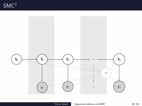
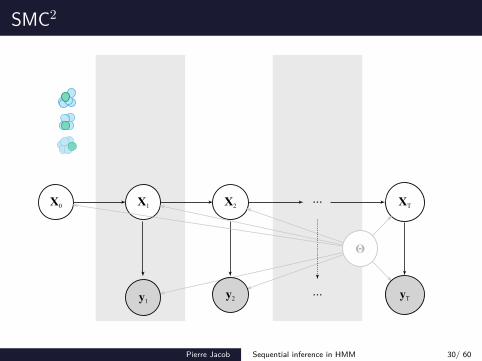
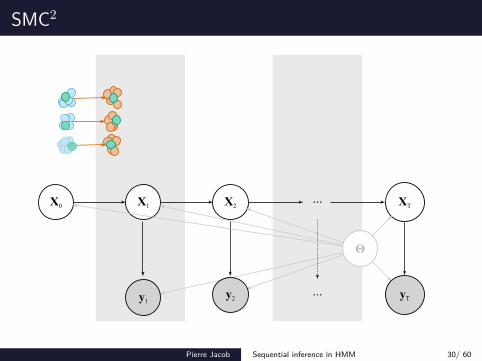
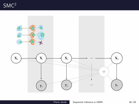
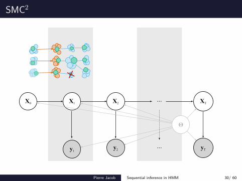
SMC2
y2
X2X0
y1
X1...
... yT
XT
Θ
Pierre Jacob Sequential inference in HMM 30/ 60
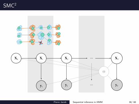
SMC2
y2
X2X0
y1
X1...
... yT
XT
Θ
Pierre Jacob Sequential inference in HMM 30/ 60
SMC2
y2
X2X0
y1
X1...
... yT
XT
Θ
Pierre Jacob Sequential inference in HMM 30/ 60
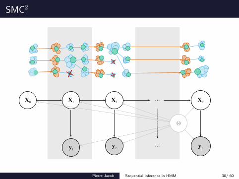
SMC2
y2
X2X0
y1
X1...
... yT
XT
Θ
Pierre Jacob Sequential inference in HMM 30/ 60
SMC2
y2
X2X0
y1
X1...
... yT
XT
Θ
Pierre Jacob Sequential inference in HMM 30/ 60
SMC2
y2
X2X0
y1
X1...
... yT
XT
Θ
Pierre Jacob Sequential inference in HMM 30/ 60
SMC2
y2
X2X0
y1
X1...
... yT
XT
Θ
Pierre Jacob Sequential inference in HMM 30/ 60
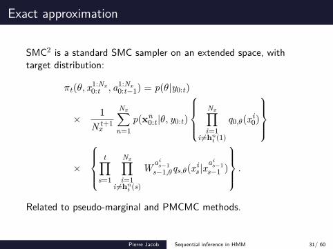
Exact approximation
SMC2 is a standard SMC sampler on an extended space, withtarget distribution:
πt(θ, x1:Nx0:t , a1:Nx
0:t−1) = p(θ|y0:t)
× 1N t+1
x
Nx∑n=1
p(xn0:t |θ, y0:t)
Nx∏i=1
i =hnt (1)
q0,θ(x i0)
×
t∏
s=1
Nx∏i=1
i =hnt (s)
W ais−1
s−1,θqs,θ(x is |x
ais−1
s−1 )
.
Related to pseudo-marginal and PMCMC methods.
Pierre Jacob Sequential inference in HMM 31/ 60
Exact approximation
From the extended target representation, we obtainθ from p(θ | y1:t),xn
0:t from p(x0:t | θ, y1:t),thus allowing joint state and parameter inference.
Evidence estimates are obtained by computing the average ofthe θ-weights ω(m)
t .
The “extended target” argument yields consistency for anyfixed Nx , when Nθ goes to infinity.
Exact method, sequential by design, but not online.
Pierre Jacob Sequential inference in HMM 32/ 60
Outline
1 Setting: online inference in time seriesHidden Markov ModelsImplicit modelsExact / sequential / online methods
2 Plug and play methodsApproximate Bayesian ComputationParticle Filters
3 SMC2 for sequential inferenceA sequential method for HMMNot online
4 Numerical experiments
5 Discussion
Pierre Jacob Sequential inference in HMM 32/ 60
Scalability in T
Cost if MCMC move at each time step
A single move step at time t costs O (tNxNθ).
If move at every step, the total cost becomes O(t2NxNθ
).
If Nx = Ct, the total cost becomes O(t3Nθ
).
With adaptive resampling, the cost is only O(t2Nθ
). Why?
Pierre Jacob Sequential inference in HMM 33/ 60
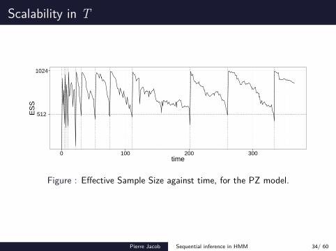
Scalability in T
512
1024
0 100 200 300time
ES
S
Figure : Effective Sample Size against time, for the PZ model.
Pierre Jacob Sequential inference in HMM 34/ 60
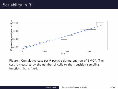
Scalability in T
0e+00
2e+06
4e+06
6e+06
0 100 200 300time
Cum
ulat
ive
cost
per
par
ticle
Figure : Cumulative cost per θ-particle during one run of SMC2. Thecost is measured by the number of calls to the transition samplingfunction. Nx is fixed.
Pierre Jacob Sequential inference in HMM 35/ 60
Scalability in T
iterations
ES
S
0
200
400
600
800
1000
1000 2000 3000 4000 5000
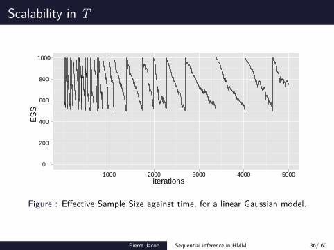
Figure : Effective Sample Size against time, for a linear Gaussian model.
Pierre Jacob Sequential inference in HMM 36/ 60
Scalability in T
iteration
com
putin
g tim
e (s
quar
e ro
ot s
cale
)
2500
10000
22500
40000
1000 2000 3000 4000 5000
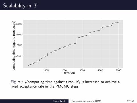
Figure :√
computing time against time. Nx is increased to achieve afixed acceptance rate in the PMCMC steps.
Pierre Jacob Sequential inference in HMM 37/ 60
Scalability in T
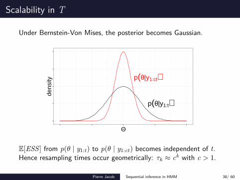
Under Bernstein-Von Mises, the posterior becomes Gaussian.
p(θ|y1:ct)
p(θ|y1:t)
Θ
dens
ity
E[ESS ] from p(θ | y1:t) to p(θ | y1:ct) becomes independent of t.Hence resampling times occur geometrically: τk ≈ ck with c > 1.
Pierre Jacob Sequential inference in HMM 38/ 60
Scalability in T
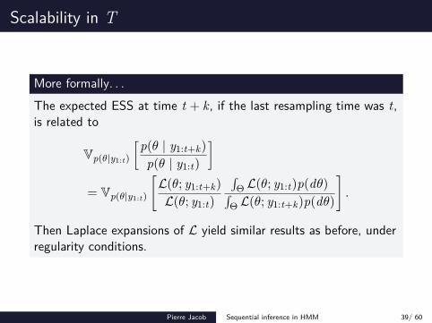
More formally. . .The expected ESS at time t + k, if the last resampling time was t,is related to
Vp(θ|y1:t)
[p(θ | y1:t+k)p(θ | y1:t)
]= Vp(θ|y1:t)
[L(θ; y1:t+k)L(θ; y1:t)
∫Θ L(θ; y1:t)p(dθ)∫
Θ L(θ; y1:t+k)p(dθ)
].
Then Laplace expansions of L yield similar results as before, underregularity conditions.
Pierre Jacob Sequential inference in HMM 39/ 60
Scalability in T
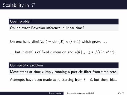
Open problemOnline exact Bayesian inference in linear time?
On one hand dim(X0:t) = dim(X )× (t + 1) which grows . . .
. . . but θ itself is of fixed dimension and p(θ | y1:t) ≈ N (θ⋆, v⋆/t)!
Our specific problemMove steps at time t imply running a particle filter from time zero.
Attempts have been made at re-starting from t −∆ but then, bias.
Pierre Jacob Sequential inference in HMM 40/ 60
Outline
1 Setting: online inference in time seriesHidden Markov ModelsImplicit modelsExact / sequential / online methods
2 Plug and play methodsApproximate Bayesian ComputationParticle Filters
3 SMC2 for sequential inferenceA sequential method for HMMNot online
4 Numerical experiments
5 Discussion
Pierre Jacob Sequential inference in HMM 40/ 60
Phytoplankton–Zooplankton: model
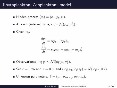
Hidden process (xt) = (αt , pt , zt).
At each (integer) time, αt ∼ N (µα, σ2α).
Given αt ,
dptdt
= αpt − cptzt ,
dztdt
= ecptzt −mlzt −mqz2t .
Observations: log yt ∼ N (log pt , σ2y).
Set c = 0.25 and e = 0.3, and (log p0, log z0) ∼ N (log 2, 0.2).
Unknown parameters: θ = (µα, σα, σy,ml ,mq).
Pierre Jacob Sequential inference in HMM 41/ 60
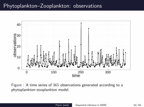
Phytoplankton–Zooplankton: observations
●●●
●
●●
●
●●●●●
●●
●
●●
●
●
●
●
●
●●●●
●
●
●
●
●●
●
●●
●●
●●
●
●
●
●
●
●
●●●●
●
●
●
●
●
●
●●●●●
●
●
●
●
●
●
●●●
●
●
●
●
●
●●●●●●
●
●
●
●●●
●
●●
●●
●
●
●●
●
●
●●
●●
●
●
●●●●
●
●●
●
●
●
●●●●●
●
●
●
●
●
●●●●
●●●●
●●
●
●
●
●
●
●
●●
●
●●
●
●
●
●●●●
●●
●
●
●
●
●●
●
●●●
●
●
●
●●●●●●
●
●●
●
●
●
●
●
●
●
●●
●
●
●
●
●●●●●●●●
●●
●
●
●
●
●●
●●●
●
●
●
●
●●●
●
●
●
●
●●●●●
●●●●
●
●
●
●
●●●
●●●
●●
●
●
●
●
●
●●
●
●●
●●●●
●●
●
●●●●●●
●
●
●●
●●
●
●●
●
●
●
●
●
●
●
●
●
●
●
●
●●●●
●
●
●
●●
●
●
●
●
●
●
●
●
●
●
●
●●
●
●●
●
●
●
●
●
●
●
●
●●●
●
●
●
●●●●
●●●
●
●
●
●
●
●
●
●●
●●
●
●
●
●
●
●●
●●●●●●
●●
●
●
●
●
●
●●●●
●
●
0
10
20
30
40
0 100 200 300time
obse
rvat
ions
Figure : A time series of 365 observations generated according to aphytoplankton–zooplankton model.
Pierre Jacob Sequential inference in HMM 42/ 60
Phytoplankton–Zooplankton: parameters
●●●●●●●●●●●●●●●●●●●●●●●●●●●●●●●●●●●●●●●●●●●●●●●●●●●●●●●●●●●●●●●●●●●●●●●●●●●●●●●●●●●●●●●●●●●●●●●●●●●●●●●●●●●●●●●●●●●●●●●●●●●●●●●●●●●●●●●●●●●●●●●●●●●●●●●●●●●●●●●●●●●●●●●●●●●●●●●●●●●●●●●●●●●●●●●●●●●●●●●●●●●●●●●●●●●●●●●●●●●●●●●●●●●●●●●●●●●●●●●●●●●●●●●●●●●●●●●●●●●●●●●●●●●●●●●●●●●●●●●●●●●●●●●●●●●●●●●●●●●●●●●●●●●●●●●●●●●●●●●●●●●●●●●●●●●●●●●●●●●●●●●●●●●●●●●●●●●●●●●●●●●●●●●●●●●●●●●●●●●●●●●●●●●●●●●●●●●●●●●●●●●●●●●●●●●●●●●●●●●●●●●●●●●●●●●●●●●●●●●●●●●●●●●●●●●●●●●●●●●●●●●●●●●●●●●●●●●●●●●●●●●●●●●●●●●●●●●●●●●●●●●●●●●●●●●●●●●●●●●●●●●●●●●●●●●●●●●●●●●●●●●●●●●●●●●●●●●●●●●●●●●●●●●●●●●●●●●●●●●●●●●●●●●●●●●●●●●●●●●●●●●●●●●●●●●●●●●●●●●●●●●●●●●●●●●●●●●●●●●●●●●●●●●●●●●●●●●●●●●●●●●●●●●●●●●●●●●●●●●●●●●●●●●●●●●●●●●●●●●●●●●●●●●●●●●●●●●●●●●●●●●●●●●●●●●●●●●●●●●●●●●●●●●●●●●●●●●●●●●●●●●●●●●●●●●●●●●●●●●●●●●●●●●●●●●●●●●●●●●●●●●●●●●●●●●●●●●●●●●●●●●●●●●●●●●●●●●●●●●●●●●●●●●●●●●●●●●●●●●●●●●●●●●●●●●●●●●●●●●●●●●●●●●●●●●●●●●●●●●●●●●●●●●●●●●●●●●●●●●●●●●●●●●●●●●●●●●●●●●●●●●●●●●●●●●●●●●●●●●●●●●●●●●●●●●●●●●●●●●●●●●●●●●●●●●●●●●●●●●●●●●●●●●●●●●●●●●●●●●●●●●●
0.60
0.65
0.70
0.75
0.80
0.45 0.50 0.55 0.60σα
µ α ●●●●●●●●●●●●●●●●●●●●●●●●●●●●●●●●●●●●●●●●●●●●●●●●●●●●●●●●●●●●●●●●●●●●●●●●●●●●●●●●●●●●●●●●●●●●●●●●●●●●●●●●●●●●●●●●●●●●●●●●●●●●●●●●●●●●●●●●●●●●●●●●●●●●●●●●●●●●●●●●●●●●●●●●●●●●●●●●●●●●●●●●●●●●●●●●●●●●●●●●●●●●●●●●●●●●●●●●●●●●●●●●●●●●●●●●●●●●●●●●●●●●●●●●●●●●●●●●●●●●●●●●●●●●●●●●●●●●●●●●●●●●●●●●●●●●●●●●●●●●●●●●●●●●●●●●●●●●●●●●●●●●●●●●●●●●●●●●●●●●●●●●●●●●●●●●●●●●●●●●●●●●●●●●●●●●●●●●●●●●●●●●●●●●●●●●●●●●●●●●●●●●●●●●●●●●●●●●●●●●●●●●●●●●●●●●●●●●●●●●●●●●●●●●●●●●●●●●●●●●●●●●●●●●●●●●●●●●●●●●●●●●●●●●●●●●●●●●●●●●●●●●●●●●●●●●●●●●●●●●●●●●●●●●●●●●●●●●●●●●●●●●●●●●●●●●●●●●●●●●●●●●●●●●●●●●●●●●●●●●●●●●●●●●●●●●●●●●●●●●●●●●●●●●●●●●●●●●●●●●●●●●●●●●●●●●●●●●●●●●●●●●●●●●●●●●●●●●●●●●●●●●●●●●●●●●●●●●●●●●●●●●●●●●●●●●●●●●●●●●●●●●●●●●●●●●●●●●●●●●●●●●●●●●●●●●●●●●●●●●●●●●●●●●●●●●●●●●●●●●●●●●●●●●●●●●●●●●●●●●●●●●●●●●●●●●●●●●●●●●●●●●●●●●●●●●●●●●●●●●●●●●●●●●●●●●●●●●●●●●●●●●●●●●●●●●●●●●●●●●●●●●●●●●●●●●●●●●●●●●●●●●●●●●●●●●●●●●●●●●●●●●●●●●●●●●●●●●●●●●●●●●●●●●●●●●●●●●●●●●●●●●●●●●●●●●●●●●●●●●●●●●●●●●●●●●●●●●●●●●●●●●●●●●●●●●●●●●●●●●●●●●●●●●●●●●●●●●●●●●●●●●
0.10
0.15
0.20
0.25
0.30
0.45 0.50 0.55 0.60σα
σ y
●●●●●●●●●●●●●●●●●●●●●●●●●●●●●●●●●●●●●●●●●●●●●●●●●●●●●●●●●●●●●●●●●●●●●●●●●●●●●●●●●●●●●●●●●●●●●●●●●●●●●●●●●●●●●●●●●●●●●●●●●●●●●●●●●●●●●●●●●●●●●●●●●●●●●●●●●●●●●●●●●●●●●●●●●●●●●●●●●●●●●●●●●●●●●●●●●●●●●●●●●●●●●●●●●●●●●●●●●●●●●●●●●●●●●●●●●●●●●●●●●●●●●●●●●●●●●●●●●●●●●●●●●●●●●●●●●●●●●●●●●●●●●●●●●●●●●●●●●●●●●●●●●●●●●●●●●●●●●●●●●●●●●●●●●●●●●●●●●●●●●●●●●●●●●●●●●●●●●●●●●●●●●●●●●●●●●●●●●●●●●●●●●●●●●●●●●●●●●●●●●●●●●●●●●●●●●●●●●●●●●●●●●●●●●●●●●●●●●●●●●●●●●●●●●●●●●●●●●●●●●●●●●●●●●●●●●●●●●●●●●●●●●●●●●●●●●●●●●●●●●●●●●●●●●●●●●●●●●●●●●●●●●●●●●●●●●●●●●●●●●●●●●●●●●●●●●●●●●●●●●●●●●●●●●●●●●●●●●●●●●●●●●●●●●●●●●●●●●●●●●●●●●●●●●●●●●●●●●●●●●●●●●●●●●●●●●●●●●●●●●●●●●●●●●●●●●●●●●●●●●●●●●●●●●●●●●●●●●●●●●●●●●●●●●●●●●●●●●●●●●●●●●●●●●●●●●●●●●●●●●●●●●●●●●●●●●●●●●●●●●●●●●●●●●●●●●●●●●●●●●●●●●●●●●●●●●●●●●●●●●●●●●●●●●●●●●●●●●●●●●●●●●●●●●●●●●●●●●●●●●●●●●●●●●●●●●●●●●●●●●●●●●●●●●●●●●●●●●●●●●●●●●●●●●●●●●●●●●●●●●●●●●●●●●●●●●●●●●●●●●●●●●●●●●●●●●●●●●●●●●●●●●●●●●●●●●●●●●●●●●●●●●●●●●●●●●●●●●●●●●●●●●●●●●●●●●●●●●●●●●●●●●●●●●●●●●●●●●●●●●●●●●●●●●●●●●●●●●●●●●●●●
0.08
0.09
0.10
0.11
0.05 0.10 0.15 0.20ml
mq
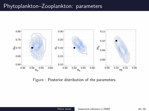
Figure : Posterior distribution of the parameters.
Pierre Jacob Sequential inference in HMM 43/ 60
Phytoplankton–Zooplankton: parameters
0.00
0.25
0.50
0.75
1.00
0 10 20 30 40 50time
µ α
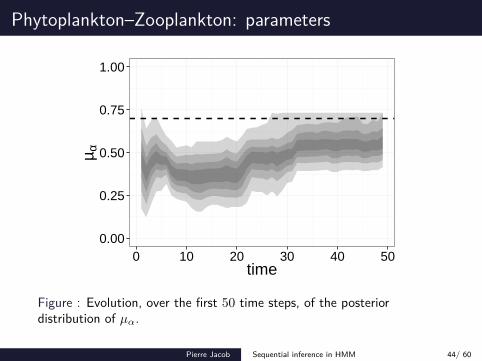
Figure : Evolution, over the first 50 time steps, of the posteriordistribution of µα.
Pierre Jacob Sequential inference in HMM 44/ 60
Phytoplankton–Zooplankton: parameters
0.00
0.25
0.50
0.75
1.00
0 10 20 30 40 50time
σ α
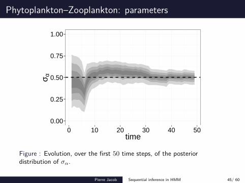
Figure : Evolution, over the first 50 time steps, of the posteriordistribution of σα.
Pierre Jacob Sequential inference in HMM 45/ 60
Phytoplankton–Zooplankton: parameters
0.00
0.25
0.50
0.75
1.00
0 10 20 30 40 50time
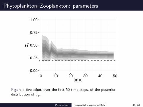
σ y
Figure : Evolution, over the first 50 time steps, of the posteriordistribution of σy.
Pierre Jacob Sequential inference in HMM 46/ 60
Phytoplankton–Zooplankton: parameters
0.00
0.25
0.50
0.75
1.00
0 10 20 30 40 50time
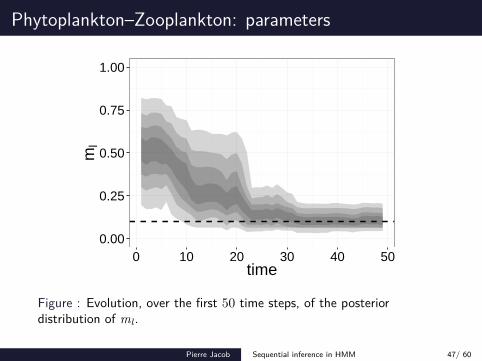
ml
Figure : Evolution, over the first 50 time steps, of the posteriordistribution of ml .
Pierre Jacob Sequential inference in HMM 47/ 60
Phytoplankton–Zooplankton: parameters
0.00
0.25
0.50
0.75
1.00
0 10 20 30 40 50time
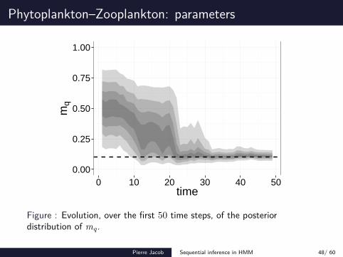
mq
Figure : Evolution, over the first 50 time steps, of the posteriordistribution of mq.
Pierre Jacob Sequential inference in HMM 48/ 60
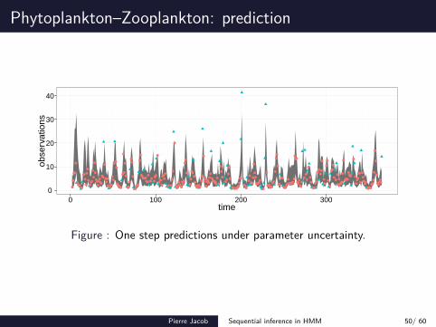
Phytoplankton–Zooplankton: prediction
●
●
● ●
●
●● ● ●
●
● ●
●
●
●
●
●
●● ●
●
●
●
●
●●
●
●●
● ●
● ●
●
●
●
●
●●
● ●
●
0
10
20
30
0 10 20 30 40 50time
obse
rvat
ions
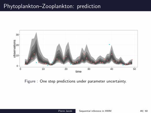
Figure : One step predictions under parameter uncertainty.
Pierre Jacob Sequential inference in HMM 49/ 60
Phytoplankton–Zooplankton: prediction
●
●
●●
●
●●●●
●
●●
●
●
●
●
●
●●●
●
●
●
●
●●●
●●●●
●●
●
●●●
●●●●
●●
●●
●
●●●●●
●
●
●
●
●
●●
●
●●
●
●●●●
●
●
●●●●●
●●
●
●●●
●
●●
●
●●●
●
●●●
●
●●●
●
●
●
●●●
●●●●
●●●
●●
●
●
●
●●●
●●●●●●
●
●
●
●●
●
●●●
●●
●●●●●
●
●
●
●
●
●
●●
●
●
●
●●●●●●●●●
●●
●●●
●
●
●●
●
●
●
●
●●●●●
●
●
●●●●●●
●●
●
●●
●
●●
●●
●●●●●
●
●●●●●●●
●●●
●●●
●●
●
●●
●
●
●
●
●●●
●●
●●
●●
●
●
●
●
●
●
●
●●
●
●●
●
●
●
●●●
●
●
●●●●
●●●
●
●
●●●
●●
●
●
●●●●
●●●●●●●●
●
●
●
●
●●●●●
0
10
20
30
40
0 100 200 300time
obse
rvat
ions
Figure : One step predictions under parameter uncertainty.
Pierre Jacob Sequential inference in HMM 50/ 60
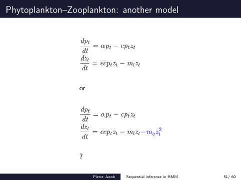
Phytoplankton–Zooplankton: another model
dptdt
= αpt − cptzt
dztdt
= ecptzt −mlzt
or
dptdt
= αpt − cptzt
dztdt
= ecptzt −mlzt−mqz2t
?
Pierre Jacob Sequential inference in HMM 51/ 60
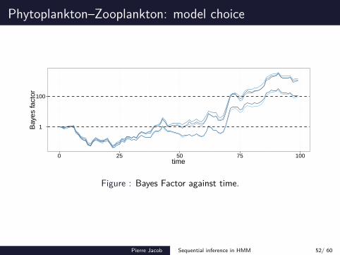
Phytoplankton–Zooplankton: model choice
1
100
0 25 50 75 100time
Bay
es fa
ctor
Figure : Bayes Factor against time.
Pierre Jacob Sequential inference in HMM 52/ 60
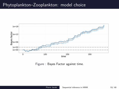
Phytoplankton–Zooplankton: model choice
1e+001e+02
1e+06
1e+12
1e+18
0 100 200 300time
Bay
es fa
ctor
Figure : Bayes Factor against time.
Pierre Jacob Sequential inference in HMM 53/ 60
Outline
1 Setting: online inference in time seriesHidden Markov ModelsImplicit modelsExact / sequential / online methods
2 Plug and play methodsApproximate Bayesian ComputationParticle Filters
3 SMC2 for sequential inferenceA sequential method for HMMNot online
4 Numerical experiments
5 Discussion
Pierre Jacob Sequential inference in HMM 53/ 60
Forgetting mechanism for hidden states
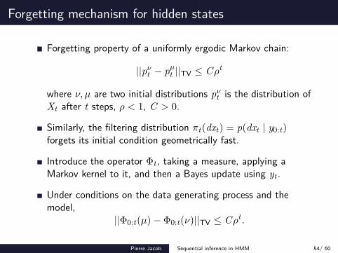
Forgetting property of a uniformly ergodic Markov chain:
||pνt − pµ
t ||TV ≤ Cρt
where ν, µ are two initial distributions pνt is the distribution of
Xt after t steps, ρ < 1, C > 0.
Similarly, the filtering distribution πt(dxt) = p(dxt | y0:t)forgets its initial condition geometrically fast.
Introduce the operator Φt , taking a measure, applying aMarkov kernel to it, and then a Bayes update using yt .
Under conditions on the data generating process and themodel,
||Φ0:t(µ)− Φ0:t(ν)||TV ≤ Cρt .
Pierre Jacob Sequential inference in HMM 54/ 60
Forgetting mechanism for parameters
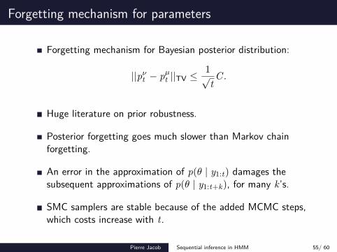
Forgetting mechanism for Bayesian posterior distribution:
||pνt − pµ
t ||TV ≤1√tC .
Huge literature on prior robustness.
Posterior forgetting goes much slower than Markov chainforgetting.
An error in the approximation of p(θ | y1:t) damages thesubsequent approximations of p(θ | y1:t+k), for many k’s.
SMC samplers are stable because of the added MCMC steps,which costs increase with t.
Pierre Jacob Sequential inference in HMM 55/ 60
Other challenges
Dimensionality: the other big open problem.
Particle filter’s errors grow exponentially fast with dim(X).
Can local particle filters beat the curse of dimensionality?Rebeschini, van Handel, 2013.
Carefully analyzed biased approximations.
Assumption of a spatial forgetting effect from the model.
Pierre Jacob Sequential inference in HMM 56/ 60
Other challenges
Particle filters provide useful estimates. . .
. . . but no estimates of their associated variance.
Can we estimate the variance without having to run thealgorithm many times?
Pierre Jacob Sequential inference in HMM 57/ 60
Other challenges
Particle methods are more and more commonly used outsidethe setting of HMMs.
For instance, in the setting of long memory processes:probabilistic programming, Bayesian non-parametricapplications.
Are particle methods useful for models that do not satisfyforgetting properties?
Stability of Feynman-Kac formulae with path-dependentpotentials,Chopin, Del Moral, Rubenthaler, 2009.
Pierre Jacob Sequential inference in HMM 58/ 60
Discussion
SMC2 allows sequential exact approximation in HMMs, butnot online.
Properties of posterior distributions could help achieving exactonline inference, or prove that it is, in fact, impossible.
Do we want to sample from the posterior as t →∞?
Importance of plug and play inference for time series.
Implementation in LibBi, with GPU support.
Pierre Jacob Sequential inference in HMM 59/ 60
Links
Particle Markov chain Monte Carlo,Andrieu, Doucet, Holenstein, 2010 (JRSS B)
Sequential Monte Carlo samplers: error bounds andinsensitivity to initial conditions,Whiteley, 2011 (Stoch. Analysis and Appl.).
SMC2: an algorithm for sequential analysis of HMM,Chopin, Jacob, Papaspiliopoulos, 2013 (JRSS B)
www.libbi.org
Pierre Jacob Sequential inference in HMM 60/ 60