current fluctuations in the open exclusion process - lapth filecurrent fluctuations in the open...

Current Fluctuations in the Open ExclusionProcess

K. Mallick and A. Lazarescu

Institut de Physique Theorique, CEA Saclay (France)

RAQIS, Angers, September 2012

K. Mallick, A. Lazarescu Current fluctuations in the Open Exclusion Process

Introduction

The statistical mechanics of a system at thermal equilibrium is encodedin the Boltzmann-Gibbs canonical law:

Peq(C) =e−E(C)/kT

Z

the Partition Function Z being related to the Thermodynamic FreeEnergy F:

F = −kTLog Z

This provides us with a well-defined prescription to analyze systems atequilibrium:(i) Observables are mean values w.r.t. the canonical measure.(ii) Statistical Mechanics predicts fluctuations (typically Gaussian) thatare out of reach of Classical Thermodynamics.


Systems far from equilibrium

No fundamental theory is yet available.

• What are the relevant macroscopic parameters?

• Which functions describe the state of a system?

• Do Universal Laws exist? Can one define Universality Classes?

• Can one postulate a general form for the microscopic measure?

• What do the fluctuations look like (‘non-gaussianity’)?

Example: Stationary driven systems in contact with reservoirs.

R1

J

R2


Rare Events and Large Deviations

Let ε1, . . . , εN be N independent binary variables, εk = ±1, withprobability p (resp. q = 1− p). Their sum is denoted by SN =

∑N1 εk .

• The Law of Large Numbers implies that SN/N → p − q a.s.

• The Central Limit Theorem implies that [SN − N(p − q)]/√

Nconverges towards a Gaussian Law.

One can show that for −1 < r < 1, in the large N limit,

Pr

(SN

N= r

)∼ e−N Φ(r)

where the positive function Φ(r) vanishes for r = (p − q).

The function Φ(r) is a Large Deviation Function: it encodes theprobability of rare events.

Φ(r) =1 + r

2ln

(1 + r

2p

)+

1− r

2ln

(1− r

2q

)


Thermodynamic Free Energy as a L. D. F.

The Large Deviation Function for density fluctuations of a gas enclosedin a box is given by

Φ(ρ) = f (ρ,T )− f (ρ0,T )− (ρ− ρ0)∂f

∂ρ0

where f = − log Z (ρ,T ) is the free energy per unit volume in units of kT .

The Free Energy of Thermodynamics can be viewed as a Large DeviationFunction

Conversely, large deviation functions may play the role of potentials innon-equilibrium statistical mechanics.

Large deviation functions obey remarkable identities that remain valid farfrom equilibrium: Fluctuation Theorem of Gallavotti and Cohen.In the vicinity of equilibrium the Fluctuation Theorem yields thefluctuation-dissipation relation (Einstein), Onsager’s relations and linearresponse theory (Kubo).


Total Current transported through an Open System

A paradigm of a non-equilibrium system

R1

J

R2

The asymmetric exclusion model with open boundaries

q 1

γ δ

1 L

RESERVOIRRESERVOIR

α β


Classical Transport in 1d: ASEP

q p p pq

Asymmetric Exclusion Process. A paradigm for non-equilibriumStatistical Mechanics.

• EXCLUSION: Hard core-interaction; at most 1 particle per site.

• ASYMMETRIC: External driving; breaks detailed-balance

• PROCESS: Stochastic Markovian dynamics; no Hamiltonian.

The probability Pt(C) to find the system in the microscopic configurationC at time t satisfies

dPt(C)

dt= MPt(C)

where the Markov Matrix M encodes the transitions rates amongstconfigurations.


ORIGINS

• Interacting Brownian Processes (Spitzer, Harris, Liggett).

• Driven diffusive systems (Katz, Lebowitz and Spohn).

• Transport of Macromolecules through thin vessels.Motion of RNA templates.

• Hopping conductivity in solid electrolytes.

• Directed Polymers in random media. Reptation models.

APPLICATIONS

• Traffic flow.

• Sequence matching.

• Brownian motors.


Representations of the quadratic algebra

The algebra encodes combinatorial recursion relations between systems ofdifferent sizes.Generically, the representations are infinite dimensional (q-deformedoscillators).

Infinite dimensional Representation:

D = 1 + d where d = q-deformed right-shift.

E = 1 + e where e = q-deformed left-shift.

D =

0√

1− q 0 0 . . .

0 0√

1− q2 0 . . .

0 0 0√

1− q3 . . .. . .

. . .

and E = D†

The matrix Ansatz allows one to calculate Stationary State Properties(currents, correlations, fluctuations) and to derive the Phase Diagram inthe infinite size limit (DEHP,1993).


The Phase Diagram

LOW DENSITY

HIGH DENSITY

MAXIMAL

CURRENT

ρ

1 − ρ

a

b

1/2

1/2

ρa = 1a++1 : effective left reservoir density.

ρb = b+

b++1 : effective right reservoir density.

a± =(1− q − α + γ)±

√(1− q − α + γ)2 + 4αγ

2α

b± =(1− q − β + δ)±

√(1− q − β + δ)2 + 4βδ

2β


Total Current

The observable Yt counts the total number of particles exchangedbetween the system and the left reservoir between times 0 and t.

Hence, Yt+dt = Yt + y with

y = +1 if a particle enters at site 1 (at rate α),

y = −1 if a particle exits from 1 (at rate γ)

y = 0 if no particle exchange with the left reservoir has occurredduring dt.

Expectation value: limt→∞〈Yt〉t = J(q, α, β, γ, δ, L) = ZL−1

ZL

The observable J represents the average-current in the stationarystate. It can be calculated by the steady-state matrix Ansatz.

Variance: limt→∞〈Y 2

t 〉−〈Yt〉2t = ∆ . This represents the fluctuations

of the total current. It requires more than the stationary measure.

Cumulant Generating Function: For t →∞, it can be proved that⟨eµYt

⟩' eE(µ)t

E (µ) encodes the statistical properties of the total current.


Large Deviations of the Current

The Large-Deviation Function Φ(j) of the total current is defined as

P

(Yt

t= j

)∼e−tΦ(j)

Using this asymptotic behaviour of the large-time PDF, one can evaluatethe average of eµYt :

〈exp(µYt)〉 '∫

dj eµtje−tΦ(j)

Hence, by the saddle-point method, we obtain that the Large-DeviationFunction and the Cumulant Generating Function E (µ) are related by aLegendre transform:

E (µ) = maxj (µj − Φ(j))


Current Statistics: Mathematical Framework

Let Pt(C,Y ) be the joint probability of being at time t in configuration Cwith Yt = Y . The time evolution of this joint probability can be deducedfrom the original Markov equation, by splitting the Markov operator

M = M0 + M+ + M−

M0 corresponds to transitions that do not modify the value of Y .

M+ are transitions that increment Y by 1: a particle enters thesystem from the left reservoir.

M− encodes rates in which Y decreases by 1, if a particle exits thesystem from the left reservoir (does not happen in the simplestTASEP case).

The Laplace transform of Pt(C,Y ) with respect to Y is defined as

Pt(C, µ) =∑Y

eµY Pt(C,Y ).


The Laplace transform Pt(C, µ) satisfies a dynamical equation governedby the deformation of the Markov Matrix M, obtained by adding ajump-counting fugacity µ:

dPt

dt= M(µ)Pt

withM(µ) = M0 + eµM+ + e−µM−

In the long time limit, t →∞, this proves the asymptotic behaviour⟨eµYt

⟩' eE(µ)t where the cumulant-generating function E (µ) is given by

the eigenvalue of M(µ) with maximal real part.

The current statistics is reduced to an eigenvalue problem, solvable byBethe Ansatz (periodic system) or by Matrix Ansatz (open system).


Analytic Procedure

Call Fµ(C) of the dominant eigenvector Fµ of M(µ). We have:

M(µ).Fµ = E (µ)Fµ

This dominant eigenvector can be formally expanded w. r. t. µ:

Fµ(C) = P(C) + µR1(C) + µ2R2(C) . . .

• For µ = 0: M(µ = 0) is the original Markov operator, E (µ = 0) = 0and P(C) is the stationary weight of the configuration C: M.P = 0.

• The generalized weight vector Rk(C) satisfies an inhomogeneouslinear equation: M.Rk = Φk (P,R1, . . .Rk−1), Φk being a linearfunctional.

• For each value of k, we show that Fµ can be represented by a matrixproduct Ansatz up to corrections of order µk+1.

• Knowing Fµ up to corrections of order µk+1, we calculate E (µ) toorder µk+1.


Generalized Matrix Ansatz

The dominant eigenvector of the deformed matrix M(µ) is given by thefollowing matrix product representation:

Fµ(C) =1

Z(k)L

〈Wk |L∏

i=1

(τiDk + (1− τi )Ek) |Vk〉+O(µk+1

)The matrices Dk and Ek are the same as above

Dk+1 = (1⊗ 1 + d ⊗ e)⊗ Dk + (1⊗ d + d ⊗ 1)⊗ Ek

Ek+1 = (1⊗ 1 + e ⊗ d)⊗ Ek + (e ⊗ 1 + 1⊗ e)⊗ Dk

The boundary vectors 〈Wk | and |Vk〉 are constructed recursively:

|Vk〉 = |β〉|V 〉|Vk−1〉 and 〈Wk | = 〈W µ|〈W µ|〈Wk−1|

[β(1− d)− δ(1− e)] |V 〉 = 0

〈W µ|[α(1 + eµ e)− γ(1 + e−µ d)] = (1− q)〈W µ|

〈W µ|[α(1− eµ e)− γ(1− e−µ d)] = 0


Structure of the solution I

For arbitrary values of q and (α, β, γ, δ), and for any system size L, thefunction E (µ) is obtained in a parametric representation

µ = −∞∑k=1

Ck(q;α, β, γ, δ, L)Bk

2k

E = −∞∑k=1

Dk(q;α, β, γ, δ, L)Bk

2k

The coefficients Ck and Dk are given by contour integrals in the complexplane:

Ck =

∮C

dz

2 i π

φk(z)

zand Dk =

∮C

dz

2 i π

φk(z)

(z + 1)2

There exists an auxiliary function

WB(z) =∑k≥1

φk(z)Bk

k

that contains the full information about the statistics of the current.K. Mallick, A. Lazarescu Current fluctuations in the Open Exclusion Process

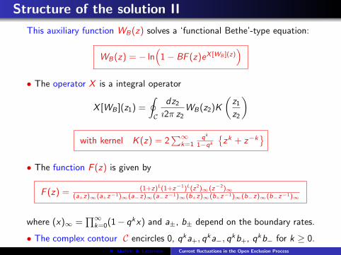
Structure of the solution II

This auxiliary function WB(z) solves a ‘functional Bethe’-type equation:

WB(z) = − ln(

1− BF (z)eX [WB ](z))

• The operator X is a integral operator

X [WB ](z1) =

∮C

dz2

ı2π z2WB(z2)K

(z1

z2

)

with kernel K (z) = 2∑∞

k=1qk

1−qk

{zk + z−k

}• The function F (z) is given by

F (z) = (1+z)L(1+z−1)L(z2)∞(z−2)∞(a+z)∞(a+z−1)∞(a−z)∞(a−z−1)∞(b+z)∞(b+z−1)∞(b−z)∞(b−z−1)∞

where (x)∞ =∏∞

k=0(1− qkx) and a±, b± depend on the boundary rates.

• The complex contour C encircles 0, qka+, qka−, q

kb+, qkb− for k ≥ 0.K. Mallick, A. Lazarescu Current fluctuations in the Open Exclusion Process

Discussion

These results are of combinatorial nature: valid for arbitrary valuesof the parameters and for any system sizes with no restrictions.

Average-Current:

J = limt→∞

〈Yt〉t

= (1− q)D1

C1= (1− q)

∮Γ

dz2 i π

F (z)z∮

Γdz

2 i πF (z)

(z+1)2

(cf. T. Sasamoto, 1999.)

Diffusion Constant:

∆ = limt→∞

〈Y 2t 〉 − 〈Yt〉2

t= (1− q)

D1C2 − D2C1

2C 31

where C2 and D2 are obtained using

φ1(z) =F (z)

2and φ2(z) =

F (z)

2

(F (z)+

∮Γ

dz2F (z2)K (z/z2)

2ıπz2

)(cf. the TASEP case: B. Derrida, M. R. Evans, K. M., 1995)


Asymptotic behaviour

Maximal Current Phase: Ek ∼ π(πL)k/2−3/2 for k ≥ 2

µ = −L−1/2

2√π

∞∑k=1

(2k)!

k!k(k+3/2)Bk

E − 1− q

4µ = − (1− q)L−3/2

16√π

∞∑k=1

(2k)!

k!k(k+5/2)Bk

Low Density (and High Density) Phases:Dominant singularity at a+: φk(z) ∼ F k(z). By Lagrange Inversion:

E (µ) = (1− q)(1− ρa)eµ − 1

eµ + (1− ρa)/ρa

Current Large Deviation Function:

Φ(j) = (1− q){ρa − r + r(1− r) ln

(1−ρaρa

r1−r

)}where the current j is parametrized as j = (1− q)r(1− r).

Matches the predictions of T. Bodineau and B. Derrida 2006, and acalculation of de Gier and Essler, 2011.


The TASEP Case (q =0)

In the case α = β = 1, the parametric representation of the cumulantgenerating function E (µ) is :

µ = −∞∑k=1

(2k)!

k!

[2k(L + 1)]!

[k(L + 1)]! [k(L + 2)]!

Bk

2k,

E = −∞∑k=1

(2k)!

k!

[2k(L + 1)− 2]!

[k(L + 1)− 1]! [k(L + 2)− 1]!

Bk

2k.

First cumulants of the current

Mean Value : J = L+22(2L+1)

Variance : ∆ = 32

(4L+1)![L!(L+2)!]2

[(2L+1)!]3(2L+3)!

Skewness :E3 = 12 [(L+1)!]2[(L+2)!]4

(2L+1)[(2L+2)!]3

{9 (L+1)!(L+2)!(4L+2)!(4L+4)!

(2L+1)![(2L+2)!]2[(2L+4)!]2 − 20 (6L+4)!(3L+2)!(3L+6)!

}For large systems: E3 → 2187−1280

√3

10368 π ∼ −0.0090978...


Full Current Statistics for the TASEP

For arbitrary (α, β), the parametric representation of E (µ) is

µ = −∞∑k=1

Ck(α, β)Bk

2k

E = −∞∑k=1

Dk(α, β)Bk

2k

with

Ck(α, β) =

∮{0,a,b}

dz

2iπ

F (z)k

zand Dk(α, β) =

∮{0,a,b}

dz

2iπ

F (z)k

(1 + z)2

where

F (z) =−(1 + z)2L(1− z2)2

zL(1− az)(z − a)(1− bz)(z − b), a =

1− αα

, b =1− ββ


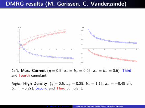
DMRG results (M. Gorissen, C. Vanderzande)

20 30 40 50 60 70 80L

- 0.004

- 0.002

0.002

0.004

0.006

E3 , E4

20 40 60 80 100L

- 0.03

- 0.02

- 0.01

0.01

0.02

0.03

0.04

E2 , E3

Left: Max. Current (q = 0.5, a+ = b+ = 0.65, a− = b− = 0.6), Thirdand Fourth cumulant.

Right: High Density (q = 0.5, a+ = 0.28, b+ = 1.15, a− = −0.48 andb− = −0.27), Second and Third cumulant.


Remarks

The function WB(z) also contains information on the 6-vertexmodel associated with the ASEP.

The periodic case falls to the same scheme:

F (z) = (1+z)L

zN

where L is the size of the system and N the conserved number ofparticles. The Kernel K (z1, z2) has the same expression.Here, the coefficients Ck and Dk are combinatorial factorsenumerating tree structures (Bethe Ansatz by S. Prolhac, 2010).

A striking coincidence: the double-series for the open TASEP of sizeL for α = 1 and β = 1/2 are identical to the formulas for thehalf-filled periodic TASEP of size 2L + 2.


Conclusion

Exact solutions of the asymmetric exclusion process are paradigms for thebehaviour of systems far from equilibrium in low dimensions: Dynamicalphase transitions, Non-Gibbsean measures, Large deviations, FluctuationsTheorems...

Large deviation functions (LDF) appear as the right generalization of thethermodynamic potentials: convex, optimized at the stationary state, andnon-analytic features can be interpreted as phase transitions. The LDF’sare very likely to play a key-role in the future of non-equilibriumstatistical mechanics.

Tensor products of quadratic algebras provides us with an efficient tool tosolve challenging problems: multispecies models; current fluctuations inthe open ASEP. In particular, the tensor matrix Ansatz gives access todensity profiles that generate atypical currents.

A. Lazarescu and K. M., J. Phys. A 44 315001 (2011)M. Gorissen, A. Lazarescu, K. M. and C. Vanderzande, PRL (Sept 2012)


current fluctuations in the open exclusion process - lapth filecurrent fluctuations in the open...

Documents