special topic

EM & Potential Methods

© 2016 EAGE www.firstbreak.org 47

first break volume 34, April 2016

CSEM anomaly identification

Neville Barker1* and Daniel Baltar1 present a simple and clear criterion to qualify a feature as anomalous with respect to its surroundings.

I n a sedimentary basin, everything typically present is highly resistive, except brine. A localized region of higher resistivity, whether identified on well logs or from con-trolled-source electromagnetic (CSEM) data, is therefore

indicative of a local reduction in interconnected brine content. This may be due to the presence of fresh water, low-porosity lithologies (including salt, volcanics and some types of carbon-ate), or hydrocarbons. It is this first-order sensitivity to fluid presence and properties that makes CSEM information of high potential value in an exploration environment (Baltar et al., 2015; Fanavoll et al., 2014; Zweidler et al., 2015).

In its simplest form, the use of CSEM for hydrocarbon detection can be considered a two-stage process. First, local-ized regions of higher resistivity need to be identified from the CSEM data. Second, these ‘anomalous’ regions must be interpreted in terms of their potential for being indicative of hydrocarbon presence. One might reasonably expect that the greater challenge is the latter: successfully predicting the geological cause of an anomalous resistivity. However, in our experience, the initial task of reliably identifying the anomalous features can prove equally challenging without an appropriate process. Early CSEM interpretation work-flows, focusing on measurement interpretation, tended to use a ‘threshold normalized amplitude response’ (NAR) rule such as 15% (Hesthammer, 2010). This proved useful in the most simple geologies, but of less value in more complex settings, and also failed to account for relative data quality. Today, the starting-point for CSEM interpretation is sub-surface resistivity images. With these, there still exists plenty

of leeway for the choice of colour scale to have a large effect on the apparent sizes of any ‘red blobs’ in the study area.

We detail here a simple and clear criterion to qualify a feature as anomalous with respect to its surroundings, which is analogous to that followed when qualifying the significance of seismic amplitude anomalies (Roden et al., 2014). We expand on an approach first proposed in Baltar and Roth, 2013, as part of a quantitative interpretation workflow for CSEM, providing a more practical guide to its application and implications. The concept is first illustrated with well data, before the method is detailed with CSEM examples.

Anomaly detection in well resistivity logsIn well analysis, we typically rely on multiple log types for interpretation. However, to draw a more strict analogy to independent CSEM interpretation, it is important to con-sider the analysis of well resistivity traces in isolation. In one-dimensional profiles of resistivity the simplest pay zones can be identified due to their outstandingly high resistivities, such as in Figure 1a. A histogram of this log (Figures 1b, 1c) shows a clear narrow ‘background’ range centered around 2.35 Wm that can be visually or algorithmically fitted to a simple distribution. In this example, we have chosen to visu-ally fit a normal distribution, which is plotted together with the histograms in Figures 1b and 1c. This distribution has a mean, m=2.35 Wm and a standard deviation, s=0.48 Wm. Given the properties of a normal distribution, this leads to a P90 of 1.74 Wm and a P10 of 2.96 Wm, as illustrated in Figure 1b.

1 EMGS.* Corresponding author, E-mail: nbarker@emgs.com

Figure 1 (a) a section of well log resistivity data, including a pay zone. (b) and (c), histograms of the same data, with a normal distribution (green) fitted to the ‘background’. Background distribution P90, P10, mean (m) and standard deviations (#s) are also labeled on (b).

special topic

EM & Potential Methods

www.firstbreak.org © 2016 EAGE48

first break volume 34, April 2016

With an interpretation for the background distribution, we now have the ability to assess the likelihood that any measure-ment is a member of this distribution, and can therefore set a criterion for how far from the background the value needs to be in order to be qualified as anomalous with high confidence. Since in this case we are using a normal distribution, we can use the simple rule that values above 3.79 Ωm (3 sigmas above background mean) only have a 0.15% chance of belonging to the background distribution. We will revisit the choice of ‘cutoff’ criterion below, in relation to CSEM data.

There are three key steps in this process:1. Identification of background resistivity.2. Fitting of background to a reasonable probability distribu-

tion.3. Moving far enough away from the background mean to

have a high confidence that measurements no longer form a part of this distribution.

Quantitative criteria can be chosen to evaluate the goodness of fit for the distribution used, and the required distance (in terms of probability) from the background to something qualifying as anomalous.

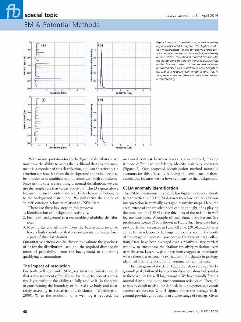
The impact of resolutionFor both well logs and CSEM, resistivity sensitivity is such that a measurement often allows for the detection of a resis-tive layer, without the ability to fully resolve it (in the sense of constraining the boundary of the resistive body and accu-rately assessing its resistivity and thickness – Worthington, 2000). When the resolution of a well log is reduced, the

measured contrast between layers is also reduced, making it more difficult to confidently identify resistivity contrasts (Figure 2). Our proposed identification method naturally accounts for this effect, by reducing the confidence in those anomalous features with a lower contrast to the background.

CSEM anomaly identificationThe CSEM measurement typically has higher resolution lateral-ly than vertically. 3D CSEM datasets therefore naturally favour interpretation in vertically averaged resistivity maps. Here, the areal extent of the resistive body can be thought of as playing the same role for CSEM as the thickness of the resistor in well log measurements. A sample of such data, from Barents Sea production licence 713, is shown in Figure 3a. These data have previously been discussed in Fanavoll et al. (2014) and Baltar et al. (2015), in relation to the Pingvin discovery, seen in the north of the image (an untested prospect at the time of data collec-tion). Data have been averaged over a relatively large vertical window to encompass the shallow resistivity variations seen over the area. Laterally, data have been cropped at boundaries where there is a reasonable expectation of a change in geology, identified from interpretation in conjunction with seismic.

The histogram of the data (Figure 3b) shows a clear ‘back-ground’ peak, followed by a potentially-anomalous tail, similar to those seen in the well log examples. We have visually fitted a normal distribution to the most common resistivities. Then, the resistivity cutoff needs to be defined. In our experience, a cutoff somewhere between 2 to 4 sigmas above the average back-ground provides good results in a wide range of settings. Given

Figure 2 Impact of resolution on a well resistivity log and associated histogram. The higher-resolu-tion measurement ((a) and (b)) shows a large con-trast between the background and high-resistivity outliers. When resolution is reduced ((c) and (d)), the background distribution remains qualitatively similar, but the contrast of the anomalous layers is reduced (seen as a reduction in peak heights in (c), and as a reduced ‘tail’ length in (d)). This, in turn, reduces the confidence in their presence and interpretability.

special topic

EM & Potential Methods

© 2016 EAGE www.firstbreak.org 49

first break volume 34, April 2016

is considered, a narrower range of resistivities is present. With a tighter color scale, a number of resistive ‘anomalies’ appear distributed across the region (Figure 3c). However, in the histogram we see that a normal distribution provides a good fit to most of the observed resistivity variation (Figure 3d). Using the same cutoff rules as above, we now transfer the P90 and P10 of the cutoff distribution on to the map view: several of the high-resistivity areas sit within the low-confidence contour, but only one area in the north-west is within the higher-confidence contour. While an interpreter may still decide to label some of these features as anomalous, there is a clear need to account for the greater chance that these are simply background resistivity variations.

there is some inherent uncertainty in where this cutoff should be placed, we choose to specify it as a normally distributed probability range, rather than a single value. We typically use a distribution width equal to the background distribution width, and a mean positioned 2.6s above the background mean. In terms of percentiles, this is equivalent to a cutoff P90 equal to the background P10. The P90 and P10 of the cutoff distribu-tion can then be treated as anomaly confidence indicators, and shown as contours on the original map view.

Small surveys, and the absence of clear anomaly-qual-ification criteria, often lead to ambiguous and uncertain interpretations. This effect can be illustrated with subsets of the above data. If only the southern portion of the data

Figure 3 (a,c,e) vertically-averaged map-views of CSEM data. (b,d,f) corresponding resistivity histo-grams, along with interpreted background and cutoff distributions. The P90 and P10 of the cutoff distributions provide the resistivity values for the anomaly confidence contours in the correspond-ing map views.

special topic

EM & Potential Methods

www.firstbreak.org © 2016 EAGE50

first break volume 34, April 2016

how this risk can be mitigated through acquisition of CSEM data over a larger area.

ReferencesBaltar, D. and Barker N.D. [2015] Prospectivity Evaluation with CSEM,

First Break 33 (9), 33-41.

Baltar, D. and Roth F. [2013] Reserves estimation methods for prospect

evaluation with 3D CSEM data: First Break 31 (6), 103–110, doi

10.3997/2214-4609.20148252.

Fanavoll, S., Gabrielsen P.T. and Ellingsrud S. [2014] CSEM as a tool

for better exploration decisions: Case studies from the Barents Sea,

Norwegian Continental Shelf: Interpretation, 2.3, SH55-SH66, doi

10.1190/INT-2013-0171.1.

Hesthammer, J., Fanavoll S., Stefatos A., Danielsen J.E. and

Boulaenko M. [2010] CSEM performance in light of well

results: The Leading Edge, 29 (1), 258–264, doi 10.1190/1.

3284051.

Roden, R., Forrest, M., Holeywell, R., Carr, M. and Alexander, P.A.

[2014] The role of AVO in prospect risk assessment. Interpretation

2.2, SC61-SC76, doi 10.1190/int-2013-0114.1.

Worthington, P.F. [2000] Recognition and evaluation of low resistivity

pay, Petroleum Geoscience, 6, 77-92.

Zweidler, D., Baltar D. and Barker N. [2015] Additional data helps

investment decisions. AAPG Explorer, November, 42-43.

Now consider a smaller region localized on the Pingvin discovery in the north (Figure 3e). This simulates a ‘single-prospect-testing’ CSEM survey, with limited coverage outside the prospect extents. The histogram now shows a wide range of common resistivities (Figure 3f). It is difficult to confidently assign a normally distributed background, and therefore the cutoff distribution is equally poorly constrained. While this result has the potential to be anomalous, analysis is pointing to the greater interpretation risk. Alternative interpretations would include:1. Large variability in regional background resistivities.2. An imaging artefact due to reduced data fold at the edges

of the small survey.Even if this is a ‘true’ anomaly, uncertainty in its quantitative evaluation will be higher, reducing the value of the CSEM information.

SummaryWe have presented a simple workflow which is designed to improve the objectivity of CSEM anomaly identification and confidence assessment. This workflow serves the same purpose as best-practice approaches for seismic amplitude anomaly interpretation. Results highlight the high interpreta-tion risk associated with single-prospect-testing surveys, and

Topics1. Seismic Survey Planning, Acquisition and Processing2. Basin Analysis and Petroleum System Modelling3. Geophysical Methods for Hydrocarbon Prospecting4. Reservoir Modelling, Characterization and Assessment5. Designing, Construction and Support of Wells Drilling6. Geological Engineering Survey7. The Experience of G&G Exploration at Okhotsk Offshore and

its Application in the Polar Region

The Fourth International Science and Applied Research Workshop

Far East Hydrocarbons 2016From Oil and Gas Basin Studies to Field Models

Call for Abstracts Deadline — 1 July 2016For more information, please contact us via e-mail: sakh@eage.org

4-6 October 2016 — Yuzhno-Sakhalinsk, Russia

www.eage.orgwww.eage.ru

18614 SAK16 170x115.indd 1 11/03/16 15:11