cse5230 - data mining, 2004lecture 9.1 data mining - cse5230 hidden markov models (hmms)...
Post on 21-Dec-2015
216 views
TRANSCRIPT

CSE5230 - Data Mining, 2004 Lecture 9.1
Data Mining - CSE5230
Hidden Markov Models (HMMs)
CSE5230/DMS/2004/9

CSE5230 - Data Mining, 2004 Lecture 9.2
Lecture Outline
Time- and space-varying processes First-order Markov models Hidden Markov models Examples: coin toss experiments Formal definition Use of HMMs for classification The three HMM problems
The evaluation problem The Forward algorithm The Viterbi and Forward-Backward algorithms
HMMs for web-mining References

CSE5230 - Data Mining, 2004 Lecture 9.3
Time- and Space-varying Processes (1)
The data mining techniques we have discussed so far have focused on the classification, prediction or characterization of single data points, e.g.: Assign a record to one of a set of classes
» Decision trees, back-propagation neural networks, Bayesian classifiers, etc.
Predicting the value of a field in a record given the values of the other fields
» Regression, back-propagation neural networks, etc. Finding regions of feature space where data points are
densely grouped
» Clustering, self-organizing maps

CSE5230 - Data Mining, 2004 Lecture 9.4
Time- and Space-varying Processes (2)
In the methods we have considered so far, we have assumed that each observed data point is statistically independent from the observation that preceded it, e.g. Classification: the class of data point xt (from time t) is
not influenced by the class of x_t-1 (from time t – 1), or indeed any other data point
Prediction: the value of a field for a record depends only on the values of the field of that record, not on values in any other records.
Several important real-world data mining problems can not be modeled in this way.

CSE5230 - Data Mining, 2004 Lecture 9.5
Time- and Space-varying Processes (3)
We often encounter sequences of observations, where each observation may depend on the observations which preceded it
Examples Sequences of phonemes (fundamental sounds) in speech
(speech recognition) Sequences of letters or words in text (text categorization,
information retrieval, text mining) Sequences of web page accesses (web usage mining) Sequences of bases (CGAT) in DNA (genome projects
[human, fruit fly, etc.)) Sequences of pen-strokes (hand-writing recognition)
In all these cases, the probability of observing a particular value in the sequence can depend on the values which came before it
CSE5230 - Data Mining, 2004 Lecture 9.6
Example: web log
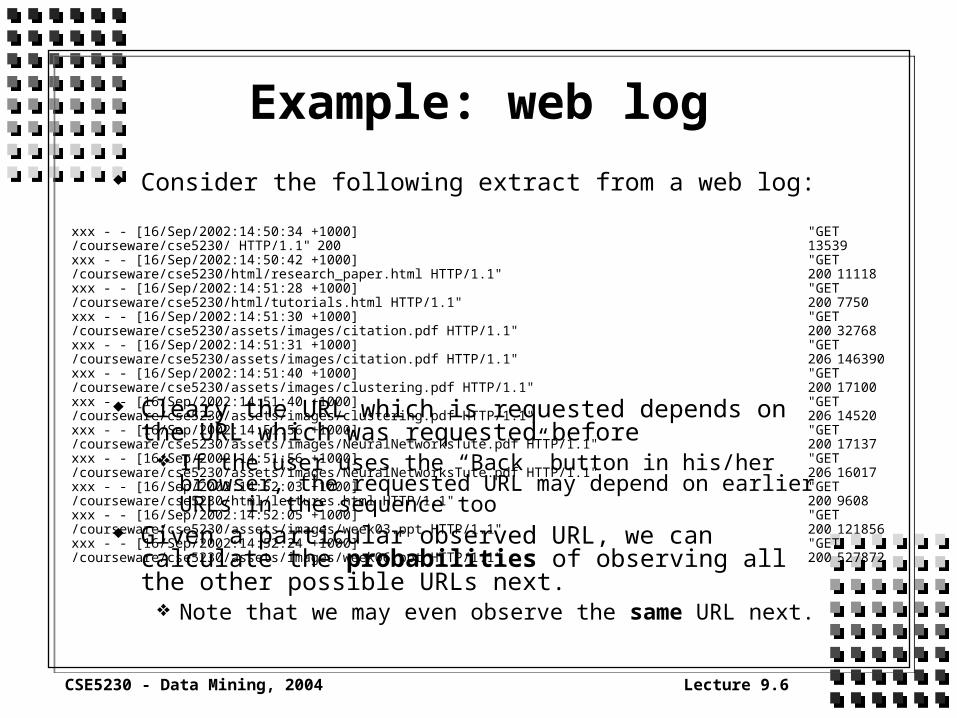
Consider the following extract from a web log:
Cleary the URL which is requested depends on the URL which was requested before
If the user uses the “Back” button in his/her browser, the requested URL may depend on earlier URLs in the sequence too
Given a particular observed URL, we can calculate the probabilities of observing all the other possible URLs next.
Note that we may even observe the same URL next.
xxx - - [16/Sep/2002:14:50:34 +1000] "GET /courseware/cse5230/ HTTP/1.1" 200 13539xxx - - [16/Sep/2002:14:50:42 +1000] "GET /courseware/cse5230/html/research_paper.html HTTP/1.1" 200 11118xxx - - [16/Sep/2002:14:51:28 +1000] "GET /courseware/cse5230/html/tutorials.html HTTP/1.1" 200 7750xxx - - [16/Sep/2002:14:51:30 +1000] "GET /courseware/cse5230/assets/images/citation.pdf HTTP/1.1" 200 32768xxx - - [16/Sep/2002:14:51:31 +1000] "GET /courseware/cse5230/assets/images/citation.pdf HTTP/1.1" 206 146390xxx - - [16/Sep/2002:14:51:40 +1000] "GET /courseware/cse5230/assets/images/clustering.pdf HTTP/1.1" 200 17100xxx - - [16/Sep/2002:14:51:40 +1000] "GET /courseware/cse5230/assets/images/clustering.pdf HTTP/1.1" 206 14520xxx - - [16/Sep/2002:14:51:56 +1000] "GET /courseware/cse5230/assets/images/NeuralNetworksTute.pdf HTTP/1.1" 200 17137xxx - - [16/Sep/2002:14:51:56 +1000] "GET /courseware/cse5230/assets/images/NeuralNetworksTute.pdf HTTP/1.1" 206 16017xxx - - [16/Sep/2002:14:52:03 +1000] "GET /courseware/cse5230/html/lectures.html HTTP/1.1" 200 9608xxx - - [16/Sep/2002:14:52:05 +1000] "GET /courseware/cse5230/assets/images/week03.ppt HTTP/1.1" 200 121856xxx - - [16/Sep/2002:14:52:24 +1000] "GET /courseware/cse5230/assets/images/week06.ppt HTTP/1.1" 200 527872

CSE5230 - Data Mining, 2004 Lecture 9.7
First-Order Markov Models (1)
In order to model processes such as these, we make use of the idea of states. At any time t, we consider the system to be in state q(t).
We can consider a sequence of successive states of length T:
qT = (q(1), q(2), …, q(T)) We will model the production of such a sequence using
transition probabilities:
Which is the probability that the system will be in state qj at time t+1 given that it was in state qi at time t
ijij atqtqP ))(|)1((
CSE5230 - Data Mining, 2004 Lecture 9.8
First-Order Markov Models (2)
A model of states and transition probabilities, such as the one we have just described, is called a Markov model.
Since we have assumed that the transition probabilities depend only on the previous state, this is a first-order Markov model Higher order Markov models are possible, but we will
not consider them here.
For example, Markov models for human speech could have states corresponding phonemes A Markov model for the word “cat” would have states
for /k/, /a/, /t/ and a final silent state

CSE5230 - Data Mining, 2004 Lecture 9.9
Example: Markov model for “cat”
/k/ /a/ /t/ /silent/
CSE5230 - Data Mining, 2004 Lecture 9.10
Hidden Markov Models
In the preceding example, we have said that the states correspond to phonemes
In a speech recognition system, however, we don’t have access to phonemes – we can only measure properties of the sound produced by a speaker
In general, our observed data does not correspond directly to a state of the model: the data corresponds to the visible states of the system
The visible states are directly accessible for measurement. The system can also have internal “hidden” states, which
can not be observed directly For each hidden state, there is a probability of observing each
visible state. This sort of model is called Hidden Markov Model (HMM)

CSE5230 - Data Mining, 2004 Lecture 9.11
Example: coin toss experiments
Let us imagine a scenario where we are in a room which is divided in two by a curtain.
We are on one side of the curtain, and on the other is a person who will carry out a procedure using coins resulting in a head (H) or a tail (T).
When the person has carried out the procedure, they call out the result, H or T, which we record.
This system will allow us to generate a sequence of Hs and Ts, e.g. HHTHTHTTHTTTTTHHTHHHHTHHHTTHHHHHHTTTTTTTTHTHHTHTTTTTHHTHTHHHTHTHHTTTTHHTTTHHTHHTTTHTHTHTHTHHHTHHTTHT….

CSE5230 - Data Mining, 2004 Lecture 9.12
Example: single fair coin Imagine that the person behind the curtain has a single fair coin
(i.e. it has equal probabilities of coming up heads or tails). This generates sequences such as
THTHHHTTTTHHHHHTHHTTHHTTHHTHHHHHHHTTHTTHHHHTHTTTHHTHTTHHHHTHTHHTTHTHTTHHTHTHHHTHHTHT…
We could model the process producing the sequence of Hs and Ts as a Markov model with two states, and equal transition probabilities:
Note that here the visible states correspond exactly to the internal states – the model is not hidden
Note also that states can transition to themselves
TH0.5
0.5
0.5
0.5
CSE5230 - Data Mining, 2004 Lecture 9.13
Example: a fair and a biased coin
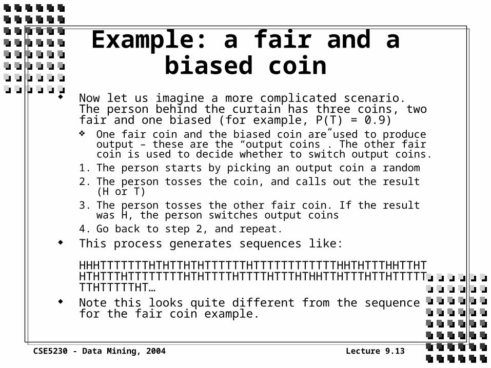
Now let us imagine a more complicated scenario. The person behind the curtain has three coins, two fair and one biased (for example, P(T) = 0.9) One fair coin and the biased coin are used to produce output –
these are the “output coins”. The other fair coin is used to decide whether to switch output coins.
1. The person starts by picking an output coin a random2. The person tosses the coin, and calls out the result (H or T)3. The person tosses the other fair coin. If the result was H, the
person switches output coins4. Go back to step 2, and repeat.
This process generates sequences like:
HHHTTTTTTTHTHTTHTHTTTTTTHTTTTTTTTTTTTHHTHTTTHHTTHTHTHTTTHTTTTTTTTHTHTTTTHTTTTHTTTHTHHTTHTTTHTTHTTTTTTTHTTTTTHT…
Note this looks quite different from the sequence for the fair coin example.
CSE5230 - Data Mining, 2004 Lecture 9.14
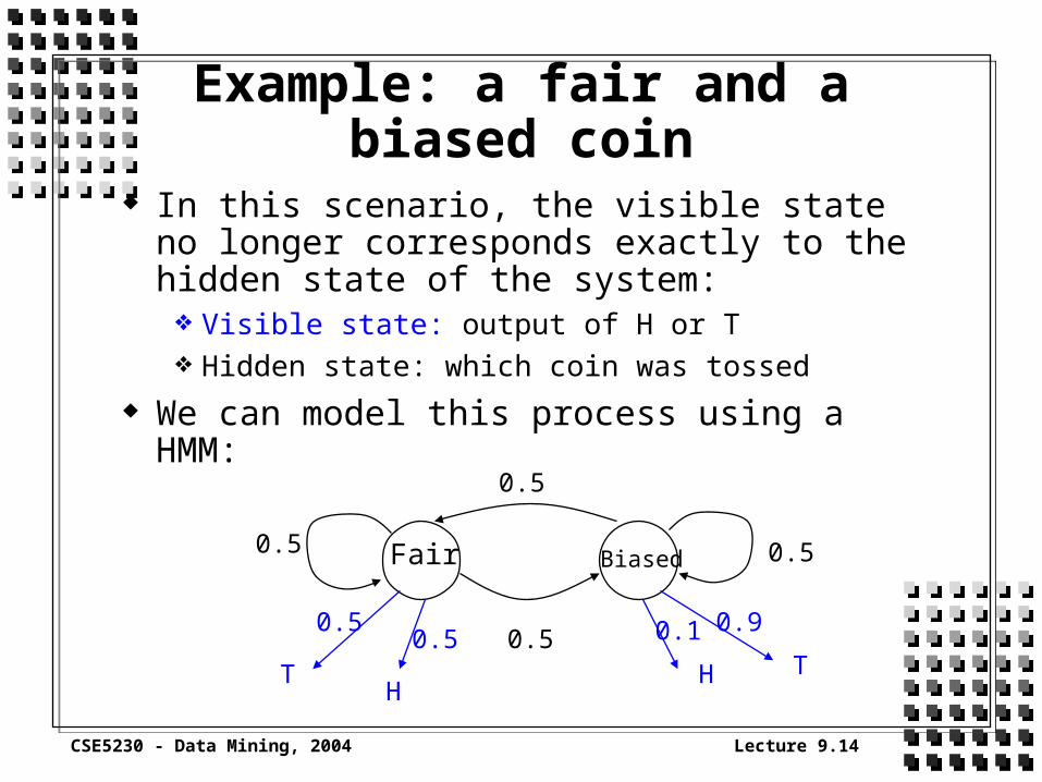
Example: a fair and a biased coin
In this scenario, the visible state no longer corresponds exactly to the hidden state of the system: Visible state: output of H or T Hidden state: which coin was tossed
We can model this process using a HMM:
BiasedFair0.5
0.5
0.5
0.50.90.10.5
0.5T
HH T
CSE5230 - Data Mining, 2004 Lecture 9.15
Example: a fair and a biased coin
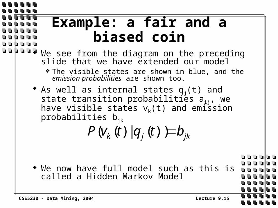
We see from the diagram on the preceding slide that we have extended our model The visible states are shown in blue, and the emission
probabilities are shown too. As well as internal states qj(t) and state transition
probabilities aij, we have visible states vk(t) and emission probabilities bjk
We now have full model such as this is called a Hidden Markov Model
jkjk btqtvP ))(|)((
CSE5230 - Data Mining, 2004 Lecture 9.16
HMM: formal definition (1)
We can now give a more formal definition of a first-order Hidden Markov Model (adapted from [RaJ1986]:
There is a finite number of (internal) states, N At each time t, a new state is entered, based upon a transition
probability distribution which depends on the state at time t – 1. Self-transitions are allowed
After each transition is made, a symbol is output, according to a probability distribution which depends only on the current state. There are thus N such probability distributions.
If we want to build an HMM to model a real sequence, we have to solve several problems. We must estimate:
the number of states N the transition probabilities aij
the emission probabilities bjk

CSE5230 - Data Mining, 2004 Lecture 9.17
HMM: formal definition (2)
When an HMM is “run”, it produces an sequence of symbols. This called an observation sequence O of length T:
O = (O(1), O(2), …, O(T))
In order to talk about using, building and training an HMM, we need some definitions:
N — the number of states in the modelM — the number of different symbols that can observed
Q = {q1, q2, …, qN} — the set of internal states
V = { v1, v2, …, vM} — the set of observable symbols
A = {aij} — the set of state transition probabilities
B = {bjk} — the set of symbol emission probabilities = {i = P(qi(1)} — the initial state probability distribution = (A, B, ) — a particular HMM model

CSE5230 - Data Mining, 2004 Lecture 9.18
Generating a Sequence
To generate an observation sequence using an HMM, we use the following algorithm:
1. Set t = 1
2. Choose an initial state q(1) according to i
3. Output a symbol O(T) according to bq(t)k
4. Choose the next state q(t + 1) according to aq(t)q(t+1)
5. Set t = t + 1; if t < T, go to 3
In applications, however, we don’t actually do this. We assume that the process that generates our data does this. The problem is to work out which HMM is responsible for a data sequence

CSE5230 - Data Mining, 2004 Lecture 9.19
Use of HMMs We have now seen what sorts of processes can be
modeled using HMMs, and how an HMM is specified mathematically.
We now consider how HMMs are actually used. Consider the two H and T sequences we saw in the
previous examples: How could we decided which coin-toss system was most likely
to have produced each sequence? To which system would you assign these sequences?
1: TTHHHTHHHTTTTTHTTTTTTHTHTHTTHHHHTHTH2: TTTTTTHTHHTHTTHTTTTHHHTHHHHTTHTHTTTT3: THTTHTTTTHTTHHHTHTTTHTHHHHTTHTHHHTHT4: TTTHHTTTHHHTTTTTTTHTTTTTHHTHTTHTTTTH
We can answer this question using a Bayesian formulation (see last week’s lecture)

CSE5230 - Data Mining, 2004 Lecture 9.20
Use of HMMs for classification HMMs are often used to classify sequences To do this, a separate HMM is built and trained (i.e. the
parameters are estimated) for each class of sequence in which we are interested
e.g. we might have an HMM for each word in a speech recognition system. The hidden states would correspond to phonemes, and the visible states to measured sound features
This gives us a set of HMMs, {l} For a given observed sequence O, we estimate the probability
that each HMM l generated it:
We assign the sequence to the model with the highest posterior probability
i.e. the probability given the evidence, where the evidence is the sequence to be classified
)(
)()|()|(
OP
POPOP ll
l

CSE5230 - Data Mining, 2004 Lecture 9.21
The three HMM problems
If we want to apply HMMs real problems with real data, we must solve three problems: The evaluation problem: given an observation
sequence O and an HMM model , compute P(O|), the probability that the sequence was produced by the model
The decoding problem: given an observation sequence O and a model , find the most likely state sequence q(1), q(2), … q(T) to have produced O
The learning problem: given a training sequence O, find a model , specified by parameters A, B, to maximize P(O|) (we assume for now that Q and V are known)
The evaluation problem has a direct solution. The others are harder, and involve optimization
CSE5230 - Data Mining, 2004 Lecture 9.22
The evaluation problem
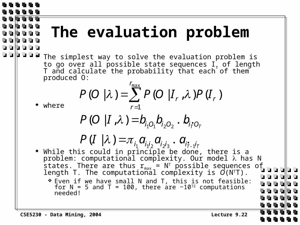
The simplest way to solve the evaluation problem is to go over all possible state sequences Ir of length T and calculate the probability that each of them produced O:
where
While this could in principle be done, there is a problem: computational complexity. Our model has N states. There are thus rmax = NT possible sequences of length T. The computational complexity is O(NTT).
Even if we have small N and T, this is not feasible: for N = 5 and T = 100, there are ~1072 computations needed!
max
1
)(),|()|(r
rrr IPIOPOP
TT
TT
iiiiiii
OiOiOi
aaaIP
bbbIOP
132211
2211
...)|(
...),|(
CSE5230 - Data Mining, 2004 Lecture 9.23
The Forward Algorithm (1)
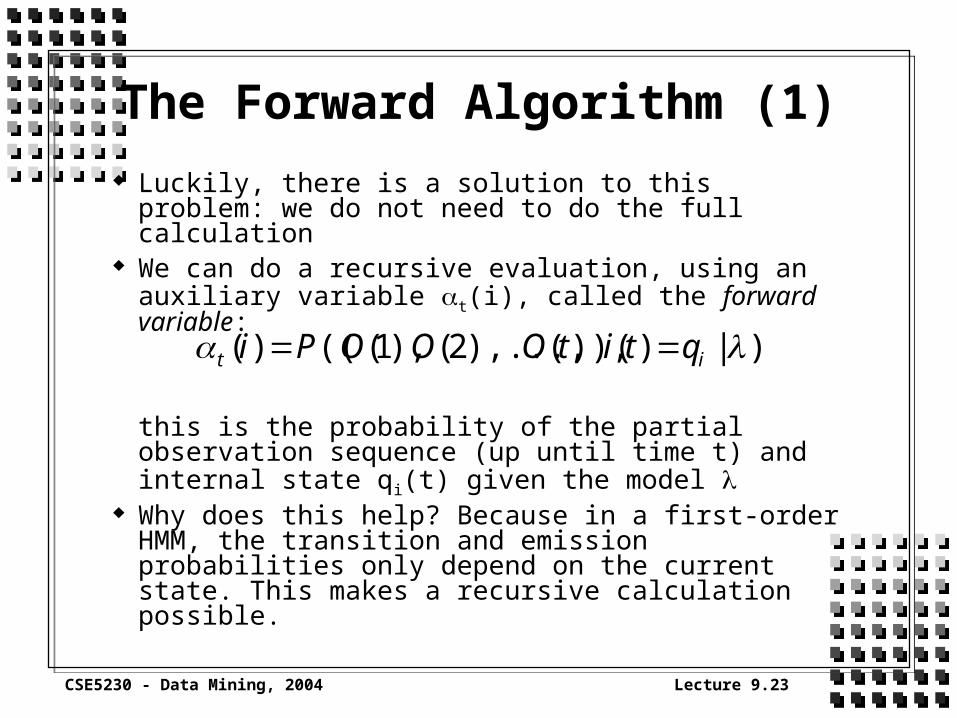
Luckily, there is a solution to this problem: we do not need to do the full calculation
We can do a recursive evaluation, using an auxiliary variable t(i), called the forward variable:
this is the probability of the partial observation sequence (up until time t) and internal state qi(t) given the model
Why does this help? Because in a first-order HMM, the transition and emission probabilities only depend on the current state. This makes a recursive calculation possible.
)|)()),(),...,2(),1((()( it qtitOOOPi

CSE5230 - Data Mining, 2004 Lecture 9.24
The Forward Algorithm (2)
We can calculate at+1(j) – the next step – using the previous one:
This just says that the probability of the observation sequence up to time t + 1 and being in state qj at time t + 1 is:
the probability of observing symbol Ot+1 when in state qj, bjOt+1, times the sum of
the probabilities of getting to state qj from state qitimes the probability of the observation sequence up to time t and being in state qi
Note that we have to keep track of t(i) for all N possible internal states
N
itijjOt iabi
t1
1 )()(1

CSE5230 - Data Mining, 2004 Lecture 9.25
The Forward Algorithm (3)
If we know T(i) for all the possible states, we can calculate the overall probability of the sequence given the model (as we wanted on slide 9.22):
We can now specify the forward algorithm, which will let us calculate the T(i):
for i = 1 to N { } /* initialize */for t = 1 to T – 1 {
for j = 1 to N {
}
}
N
iT iOP
1
)()|(
1)(1 iOibi
N
itijjOt iabi
t1
1 )()(1
CSE5230 - Data Mining, 2004 Lecture 9.26
The Forward Algorithm (4)
The forward algorithm allows us to calculate P(O|), and has computational complexity O(N2T), as can be seen from the algorithm This is linear in T, rather than exponential, as the direct
calculation was. This means that it is feasible
We can use P(O|) in the Bayesian equation on slide 9.20 to use a set of HMMs a classifier The other terms in the equation can be estimated from
the training data, as with the Naïve Bayesian Classifier
CSE5230 - Data Mining, 2004 Lecture 9.27
The Viterbi and Forward-Backward Algorithms
The most common solution to the decoding problem uses the Viterbi algorithm [RaJ1986], which also uses partial sequences and recursion
There is no known method for finding an optimal solution to the learning problem. The most commonly used optimization technique is known as the forward-backward algorithm, or the Baum-Welch algorithm [RaJ1986,DHS2000]. It is a generalized expectation maximization algorithm. See references for details

CSE5230 - Data Mining, 2004 Lecture 9.28
HMMs for web-mining (1)
HMMs can be used to analyse to clickstreams the web users leave in the log files of web servers (see slide 9.6).
Ypma and Heskes (2002) report the application of HMMs to: Web page categorization User clustering
They applied their system to real-word web logs from a large Dutch commercial web site [YpH2002]

CSE5230 - Data Mining, 2004 Lecture 9.29
HMMs for web-mining (2)
A mixture of HMMs is used to learn page categories (the hidden state variables) and inter-category transition probabilities The page URLs are treated as the observations
Web surfer types are modeled by HMMs A clickstream is modeled as a mixture of HMMs,
to account for several types of user being present at once

CSE5230 - Data Mining, 2004 Lecture 9.30
HMMs for web-mining (3)
When applied to data from a commercial web site, page categories were learned as hidden states
Inspection of the emission probabilities B showed that several page categories were discovered:
» Shop info» Start, customer/corporate/promotion» Tools» Search, download/products
Four user types were discovered too (HMMs with different state prior and transition probabilities)
Two types dominated:» General interest users» Shop users
The starting state was the most important difference between the types

CSE5230 - Data Mining, 2004 Lecture 9.31
References [DHS2000] Richard O. Duda, Peter E. Hart and David
G. Stork, Pattern Classification (2nd Edn), Wiley, New York, NY, 2000, pp. 128-138
[RaJ1986] L. R. Rabiner and B. H. Juang, An introduction to hidden Markov models, IEEE Magazine on Acoustics, Speech and Signal Processing, 3, 1, pp. 4-16, January 1986.
[YpH2002] Alexander Ypma and Tom Heskes, Categorization of web pages and user clustering with mixtures of hidden Markov models, In Proceedings of the International Workshop on Web Knowledge Discovery and Data mining (WEBKDD'02), Edmonton, Canada, July 17 2002.