cse461 constraint logic programming (clp) u logic programming u clp programs u evaluation of clp...
Post on 22-Dec-2015
249 views
TRANSCRIPT

CSE461Constraint Logic Programming (CLP)
Logic programming CLP programs Evaluation of CLP programs The CLP class of programming languages Using data structures Modelling with finite domain constraints Optimisation in CLP advanced programming techniques
Based on
Chapters 4, 5, 6 & 8 of Marriott & Stuckey

Constraint Logic Programs (CLP)
Constraint logic programs (CLP) have simple syntax yet allow flexible modelling of constraint problems.
The most basic construct in a CLP program is a rule (similar to a procedure definition).
% abs(X,Y) holds if Y = |X|abs(X,Y) :- X ≥ 0, Y = X.abs(X,Y) :- X < 0, Y = -X.
This defines a user defined constraint (also called a predicate). In this case abs (or more exactly abs/2).
A CLP program is simply a collection of rules.
and
comment
if

Constraint Logic Programs (Cont.)
We can have complex expressions in the head of the rule. abs(X,X) :- X ≥ 0.abs(X,-X) :- X < 0.
We can call user defined constraints in the body of the rule.
abs(X,X) :- X ≥ 0.abs(X,Y) :- neg(X,Y).neg(X,-X).
A rule without a body is called a fact.
body
head
fact
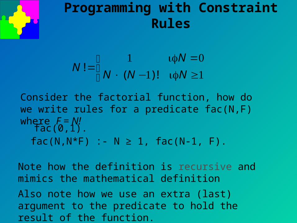
Programming with Constraint Rules
Consider the factorial function, how do we write rules for a predicate fac(N,F) where F = N!
NN
N N N!
( )!=
=× − ≥
⎧⎨⎩
1 01 1
if if
fac(0,1). fac(N,N*F) :- N ≥ 1, fac(N-1, F).
Note how the definition is recursive and mimics the mathematical definition
Also note how we use an extra (last) argument to the predicate to hold the result of the function.
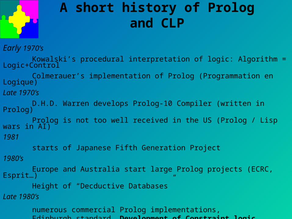
A short history of Prolog and CLP
Early 1970’s
Kowalski’s procedural interpretation of logic: Algorithm = Logic+Control
Colmerauer’s implementation of Prolog (Programmation en Logique)
Late 1970’s
D.H.D. Warren develops Prolog-10 Compiler (written in Prolog)
Prolog is not too well received in the US (Prolog / Lisp wars in AI)
1981
starts of Japanese Fifth Generation Project
1980’s
Europe and Australia start large Prolog projects (ECRC, Esprit…)
Height of “Decductive Databases”
Late 1980’s
numerous commercial Prolog implementations, Edinburgh standard, Development of Constraint logic Programming
Late 1980’s / 1990’s
Prolog widely used in AI

History of CLP
SKETCHPAD (Sutherland, 1963)
CONSTRAINTS (Steele, 1980)
ThingLab (Borning, 1981)
Prolog (Colmeraur, 1972)
Prolog II (Colmeraur, 1982)
CLP Scheme & CLP(R) (Jaffar & Lassez, 1987)
CHIP (Dincbas & Van Hentenryck
1988)
Prolog III (Colmeraur, 1987
Lots of CLP Languages Eclipse, SICStus Prolog, HAL..
ILOG Solver (Puget, 1994)

The Roots: Database Programming
In Prolog:
married(couple1, benjamin, stella).married(couple2, lisa, scott).married(couple3, tom, lydia).
child(couple1, roger).child(couple1, lisa).child(couple2, tom).child(couple2, martin).
ChildrenCouple Childcouple1 rogercouple1 lisacouple2 tomcouple2 martin
MarriageCouple Husband Wifecouple1 benjamin stellacouple2 scott lisa couple3 tom lydia
Queries:
“Who is Lisa married to?”?- married(Couple, Husband, lisa).
-> Husband=scott, Couple=couple2
“Who are the Children of Lisa and Scott?”?- child(couple2, Child).
-> Child=tom-> Child=martin
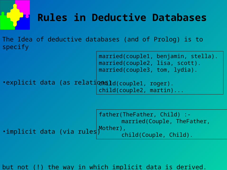
Rules in Deductive Databases
The Idea of deductive databases (and of Prolog) is to specify
•explicit data (as relations)
•implicit data (via rules)
but not (!) the way in which implicit data is derived.
married(couple1, benjamin, stella).married(couple2, lisa, scott).married(couple3, tom, lydia).
child(couple1, roger).child(couple2, martin)...
father(TheFather, Child) :- married(Couple, TheFather, Mother),child(Couple, Child).

Logic Programming
The dream of Declarative Programming
- don’t program how to find solution
- model the problem and use a universal problem
solving procedure to find the solution
Algorithm = Logic + Control
...obviously this is also what one wants from a modelling language
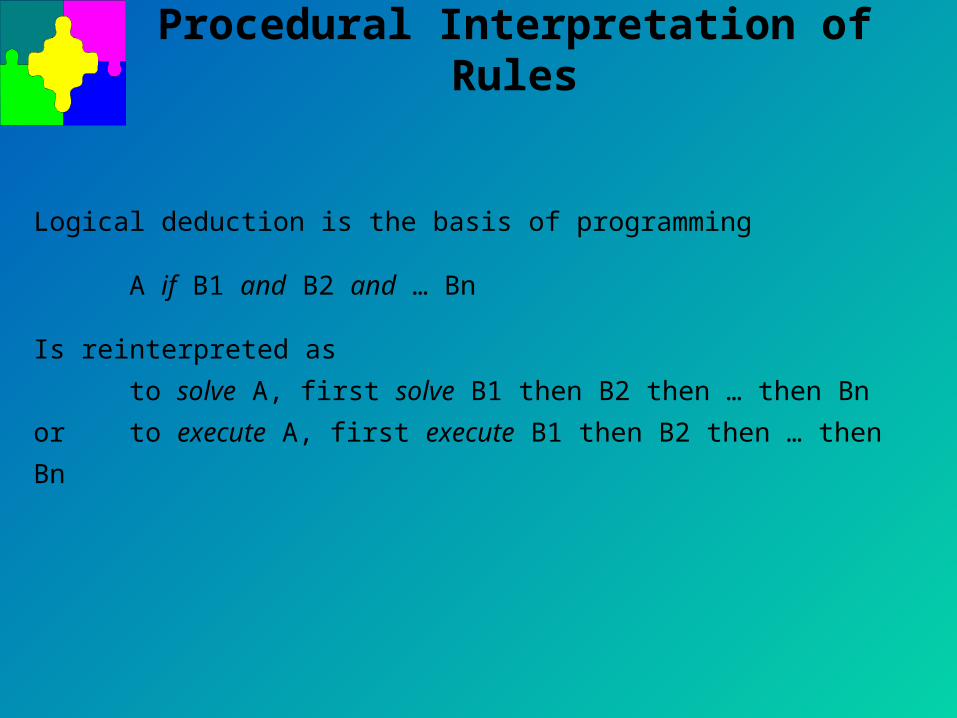
Procedural Interpretation of Rules
Logical deduction is the basis of programming
A if B1 and B2 and … Bn
Is reinterpreted as
to solve A, first solve B1 then B2 then … then Bn
or to execute A, first execute B1 then B2 then … then Bn
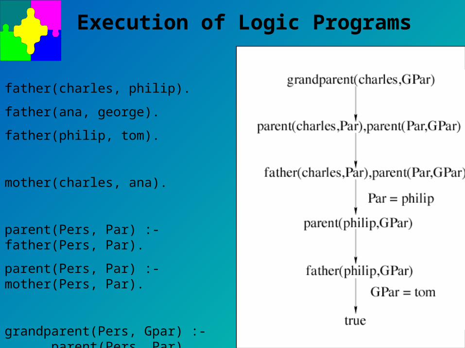
Execution of Logic Programs
father(charles, philip).
father(ana, george).
father(philip, tom).
mother(charles, ana).
parent(Pers, Par) :- father(Pers, Par).
parent(Pers, Par) :- mother(Pers, Par).
grandparent(Pers, Gpar) :-parent(Pers, Par), parent(Par, Gpar).

Simplified Interpreter (ground goals)
Input: A ground goal G and a program P
Output: yes if G is a consequence of P (“is true in P”),
no otherwise
Initialize resolvent to G
Algorithm:
While (resolvent A1, …, An is not empty) do
choose a goal A from the resolvent
choose a ground instance of a clause
A’ :- B1, …, Bn from P
such that A and A’ are identical
(exit with “no” if no such clause)
replace A by B1, …, Bn in the resolvent
If (resolvent is empty) answer “yes” else answer “no”
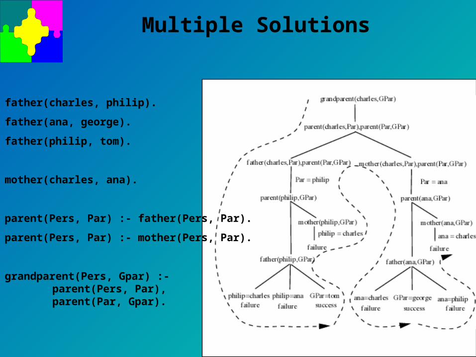
Multiple Solutions
father(charles, philip).
father(ana, george).
father(philip, tom).
mother(charles, ana).
parent(Pers, Par) :- father(Pers, Par).
parent(Pers, Par) :- mother(Pers, Par).
grandparent(Pers, Gpar) :-parent(Pers, Par), parent(Par, Gpar).

Recursion
ancestor(P, Anc) :- parent(P, Anc).
ancestor(P, Anc) :- parent(P, Par), ancestor(Par, Anc).
father(charles,philip).
father(ana,george).
father(philip,tom).
mother(charles,ana).

Evaluating CLP Programs
A CLP program is evaluated by running a goal which is a sequence of literals (I.e. user defined constraints and primitive constraints).
The leftmost user-defined constraint is repeatedly replaced by its definition until no user defined constraints are left.
The resulting constraint is simplified in terms of the variables in the original goal: it is called an answer to the goal.
Conceptually the rules act like macro definitions: the head of the rule is replaced by the body of the rule.

Evaluating CLP Programs--Example
(R1) fac(0,1).(R2) fac(N,N*F) :- N >= 1, fac(N-1, F).
Rewriting the goal fac(2,X) (i.e. what is 2!)fac X( , )2fac X
R
N X N F N fac N F
( , )
, , , ( , )
2
2
2 1 1
⇓= = × ≥ −
fac X
R
N X N F N fac N F
R
N X N F N N N F N F N fac N F
( , )
, , , ( , )
, , , ' , ' ' , ' , ( ' , ' )
2
2
2 1 1
2
2 1 1 1 1
⇓= = × ≥ −
⇓= = × ≥ − = = × ≥ −
fac X
R
N X N F N fac N F
R
N X N F N N N F N F N fac N F
R
N X N F N N N F N F N N F
( , )
, , , ( , )
, , , ' , ' ' , ' , ( ' , ' )
, , , ' , ' ' , ' , ' , '
2
2
2 1 1
2
2 1 1 1 1
1
2 1 1 1 1 0 1
⇓= = × ≥ −
⇓= = × ≥ − = = × ≥ −
⇓= = × ≥ − = = × ≥ − = =
Simplified onto variable X, then answer X = 2Different rewriting: the constraints are unsatisfiable
fac X
R
N X N F N fac N F
R
N X N F N N N F N F N fac N F
R
N X N F N N N F N F N
N N F N F N fac N F
( , )
, , , ( , )
, , , ' , ' ' , ' , ( ' , ' )
, , , ' , ' ' , ' ,
' ' ' , ' ' ' ' ' , ' ' , ( ' ' , ' ' )
2
2
2 1 1
2
2 1 1 1 1
2
2 1 1 1
1 1 1
⇓= = × ≥ −
⇓= = × ≥ − = = × ≥ −
⇓= = × ≥ − = = × ≥
− = = × ≥ −

Evaluating CLP Programs (Cont.)
Evaluation is a little more complex than this: We have to rename the rules (so as to avoid name
conflicts with local variables) and add equations to equate the formal and actual parameters
For efficiency it is better to repeatedly test the primitive constraints encountered so far for satisfiability, as if they are unsatisfiable we can stop with failure.
To do this we collect the primitive constraints in a constraint store and whenever the leftmost literal is a primitive constraint this is added to the store and tested by the (incremental) constraint solver for satisfiability.

Evaluating CLP Programs (Cont.)
There may be more than one rule defining the same user-defined constraint. (This encodes choice).
In this case the rules are tried in turn. Once one definition leads to failure, the system backtracks and tries the next rule in the definition.
Once an answer is found, the CLP system returns. The user can request the next answer, in which case the system backtracks to find the next.
If all choices lead to failure, the goal is said to have finitely failed, and no is returned.

Evaluating CLP Programs--Example
(R1) abs(X,X) :- X ≥ 0.(R2) abs(X,-X) :- X < 0.
Evaluate the goal abs(- 4,Y):
<abs(-4,Y) | true>
goal
Constraint store
<-4=X, Y=X, X≥0 | true>
(R1)
<Y=X, X≥0 | -4=X>
< X≥0 | -4=XY=X>
failure
<-4=X, Y=-X, X<0 | true>
(R2)
<Y=-X, X<0 | -4=X>
<X<0 | -4=X Y=-X>
<nil| -4=X Y=-X X<0>
simplify in terms of Y giving answer Y=4

The CLP Scheme
We have actually introduced the CLP scheme. This defines a family of programming languages A language CLP(X) is defined by
constraint domain X solver for the constraint domain X
We have been using CLP(Real) Prolog is actually CLP(Tree)
This provides equality over terms (or trees). Their combination is CLP(R). This provides equality over
terms (or trees) and arithmetic constraints over the reals. CLP(FD) provides finite domain constraints.

Data Structures
CLP languages inherit data structures from Prolog: Records Lists Trees
Data structures are terms They are accessed and manipulated using term constraints
--they are just another constraint domain! There are no type declarations
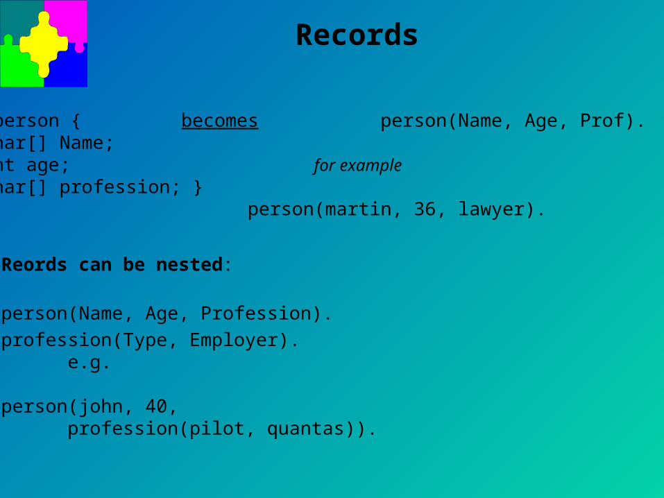
Records
Reords can be nested:
person(Name, Age, Profession).
profession(Type, Employer).e.g.
person(john, 40,profession(pilot, quantas)).
Struct person { becomes person(Name, Age, Prof).char[] Name;int age; for examplechar[] profession; }
person(martin, 36, lawyer).
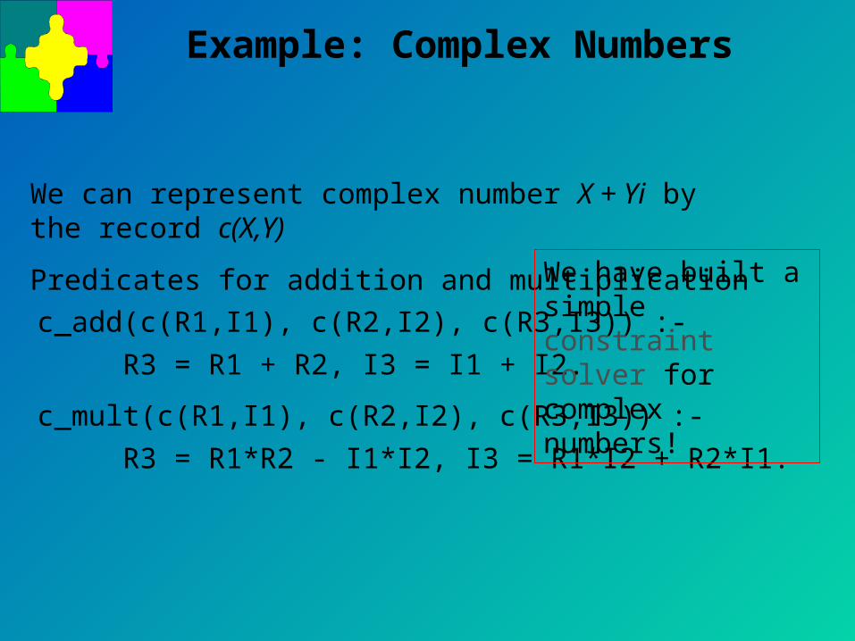
Example: Complex Numbers
We can represent complex number X + Yi by the record c(X,Y)
Predicates for addition and multiplication
c_add(c(R1,I1), c(R2,I2), c(R3,I3)) :-
R3 = R1 + R2, I3 = I1 + I2.
c_mult(c(R1,I1), c(R2,I2), c(R3,I3)) :-
R3 = R1*R2 - I1*I2, I3 = R1*I2 + R2*I1.
We have built a simple constraint solver for complex numbers!
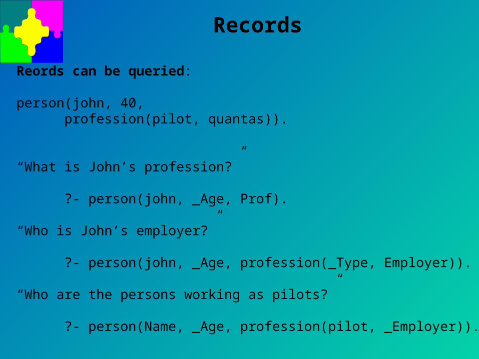
Records
Reords can be queried:
person(john, 40,profession(pilot, quantas)).
“What is John’s profession?”
?- person(john, _Age, Prof).
“Who is John’s employer?”
?- person(john, _Age, profession(_Type, Employer)).
“Who are the persons working as pilots?”
?- person(Name, _Age, profession(pilot, _Employer)).

Equality Constraints on Terms Unification
•In (constraint) logic programming there are no assignments
X = Y means “ make X and Y equal, but keep them as general as possible”
X=abc => X=abcabc=X => X=abcX=Y => no change,
but both variables identical (as if X=_1, Y=_1)
f(a)=f(X) => X=af(a,Y)=f(X,X) => X=Y and X=Y=af(X)=X => ??????? (not permitted). except in Prolog III)
Unification computes the most general substitution required to make the terms equal
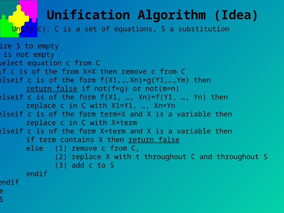
Unification Algorithm (Idea)Unify(C): C is a set of equations, S a substitution
Initialize S to emptyWhile C is not empty
select equation c from Cif c is of the from X=X then remove c from Celseif c is of the form f(X1,…,Xn)=g(Y1,…,Ym) then
return false if not(f=g) or not(m=n)elseif c is of the form f(X1, …, Xn)=f(Y1, …, Yn) then
replace c in C with X1=Y1, …, Xn=Ynelseif c is of the form term=X and X is a variable then
replace c in C with X=termelseif c is of the form X=term and X is a variable then
if term contains X then return falseelse (1) remove c from C,
(2) replace X with t throughout C and throughout S(3) add c to S
endifendif
endwhilereturn S
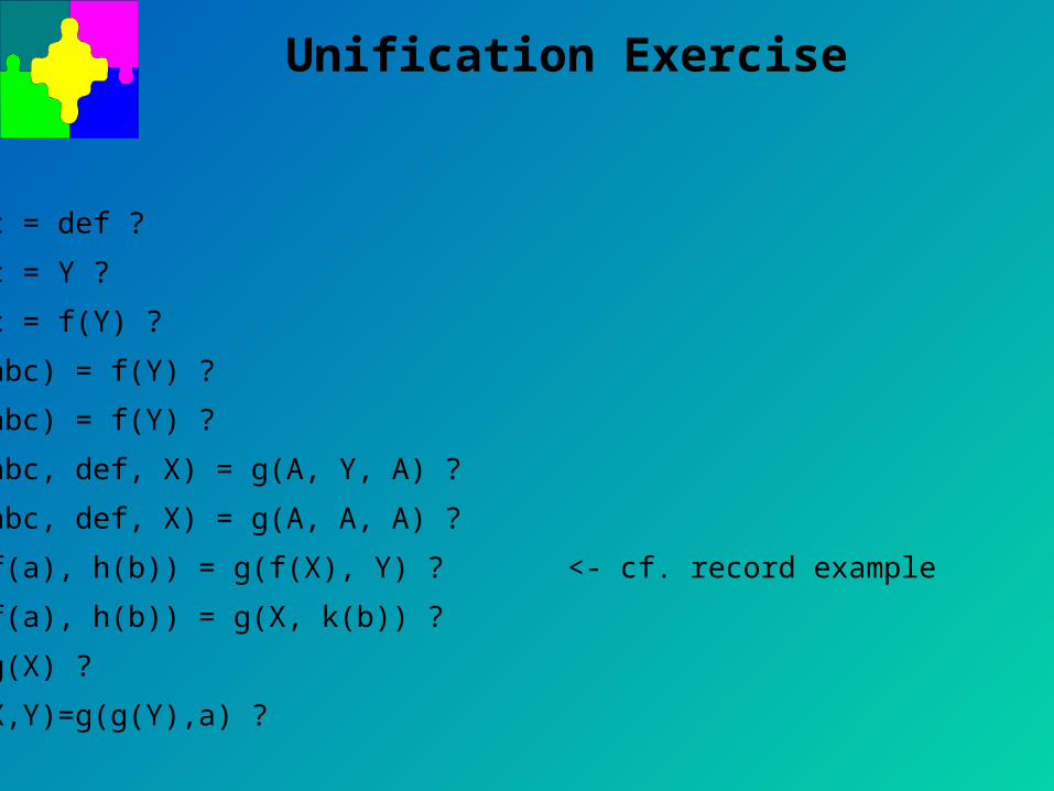
Unification Exercise
•abc = def ?
•abc = Y ?
•abc = f(Y) ?
•f(abc) = f(Y) ?
•g(abc) = f(Y) ?
•g(abc, def, X) = g(A, Y, A) ?
•g(abc, def, X) = g(A, A, A) ?
•g(f(a), h(b)) = g(f(X), Y) ? <- cf. record example
•g(f(a), h(b)) = g(X, k(b)) ?
•X=g(X) ?
•g(X,Y)=g(g(Y),a) ?
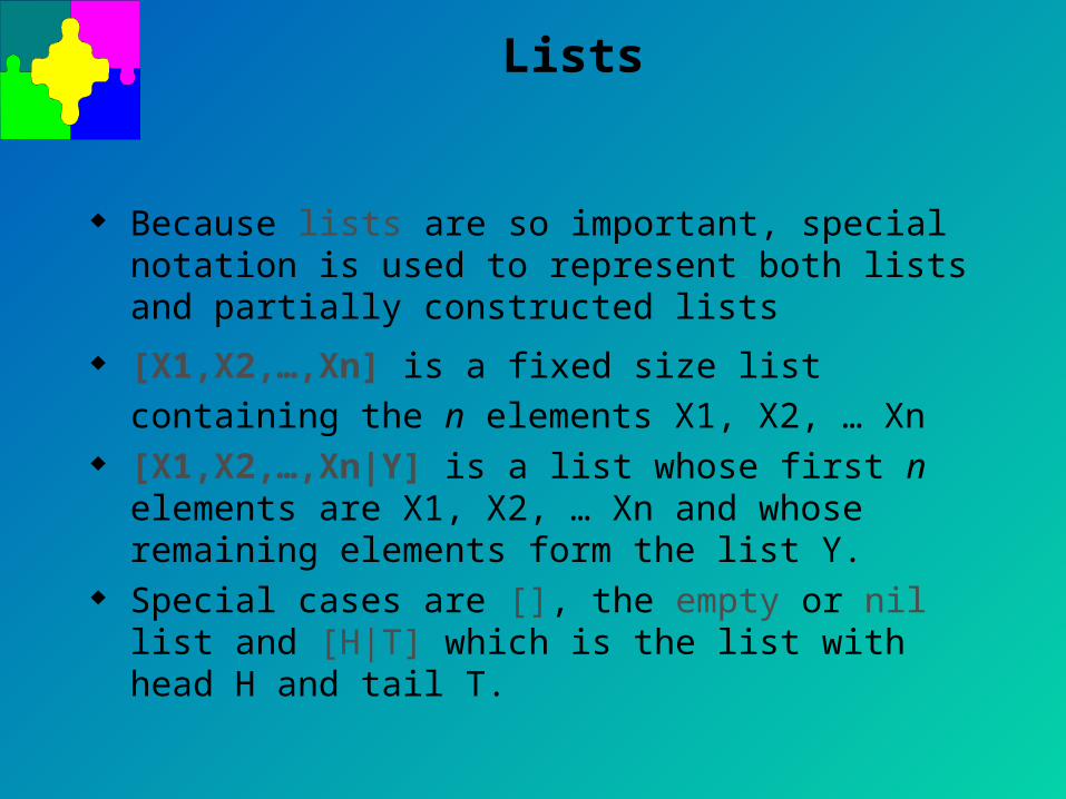
Lists
Because lists are so important, special notation is used to represent both lists and partially constructed lists
[X1,X2,…,Xn] is a fixed size list containing the n
elements X1, X2, … Xn [X1,X2,…,Xn|Y] is a list whose first n elements are X1,
X2, … Xn and whose remaining elements form the list Y. Special cases are [], the empty or nil list and [H|T] which
is the list with head H and tail T.
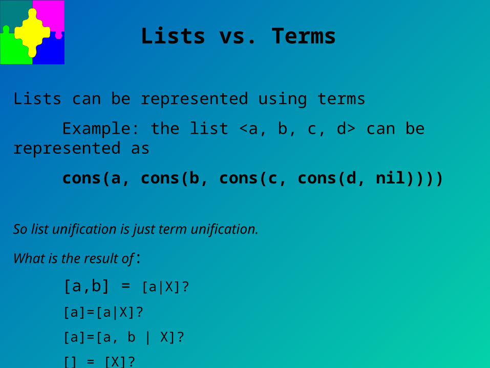
Lists vs. Terms
Lists can be represented using terms
Example: the list <a, b, c, d> can be represented as
cons(a, cons(b, cons(c, cons(d, nil))))
So list unification is just term unification.
What is the result of:
[a,b] = [a|X]?
[a]=[a|X]?
[a]=[a, b | X]?
[] = [X]?

Programming with Lists
CLP languages do not provide iteration, only recursion. The key to programming with lists is to reason recursively
about the list Either the list is empty, and the operation of interest
should be straightforward, or It is non-empty and can be broken into a first element
(the head) and the remaining list (the tail) which is dealt with recursively.

List Membership
Define a constraint, member(X,L), which holds if X is an element of list L.
Key: reason about two cases for L L is [ ], fail L is [H|T]:
if H is X then true, or if X is an element of T it is true.
member(X,[]) :- fail.
member(X, [H|T]) :- X=H.member(X, [H|T]) :- member(X,T).
member(X, [X|_]).member(X, [_|T]) :- member(X,T).

Membership Examples
member(X, [X|_]).member(X, [_|T]) :- member(X,T).
• Is X a member of L? ?- member(1,[2,3,1,4]).
Yes
•What are the elements in L??- member(X,[2,3,1,4]).
X=2; X=3; X=1; X=4; no (more answers)
•What lists contain X as an element??- member(X,L).
L=[X|_]; L=[_,X|_]; L=[_,_,X|_]; ...
Notice how member behaves as a constraint rather than as a function

member/3
We can also define a predicate member(X,L,R) that checks whether an
element X is in the List L and unifies R with L after removal of X
member(X, [X | Rest], Rest).
member(X, [_ | Rest], Rest1) :- member(X, Rest, Rest1).
Analyze: member(X, [a,b], R).member(a, [a,b,a,c], R).member(c, [a,b], R).
This does not achieve the desired effect, because it looses elements in front of the item that we are looking for!

member/3: Corrected
member(X, [X | Rest], Rest).
member(X, [F | Rest], [F | Rest1]) :- member(X, Rest, Rest1).
Analyze: member(X, [a,b], R).member(a, [a,b,a,c], R).member(c, [a,b], R).
This no longer “discards” items that are not the search element,but keeps track of them in F.The base case remains unchanged.
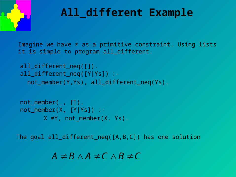
All_different Example
Imagine we have ≠ as a primitive constraint. Using lists it is simple to program all_different.
all_different_neq([]).all_different_neq([Y|Ys]) :-
not_member(Y,Ys), all_different_neq(Ys).
The goal all_different_neq([A,B,C]) has one solution
A B A C B C≠ ∧ ≠ ∧ ≠
not_member(_, []).not_member(X, [Y|Ys]) :-
X ≠Y, not_member(X, Ys).

append/3
A frequently needed operation is the concatenation of two lists:
append(L1, L2, L3) is defined such that L3 is the concatenation of L1 and L2
append([], L2, L2).append([X | Rest], L2, [X | Result]) :- append(Rest, L2, Result).

append/3
What happens with the following queries?
append([a,b],[c,d], Result). Yes!append(X, [b,c], [a,b,c]). Yes!append(X, Y, [a,b,c]). Yes, generates all possible solutions
append(L1, [], Result). No!because first and third argumentcan infinitely be extended
The recursion tries to shorten the first and third argument. This must eventually terminate to reach base case or to fail.
append([], L2, L2).append([X | Rest], L2, [X | Result]) :- append(Rest, L2, Result).

reverse/3
As defined here, reverse is hideously inefficient,Because append has to traverse the list.
We will see a better solution soon...
a predicate to reverse the order of the elements in a list:
reverse([], []).reverse([H | T ], L) :-
reverse(T, RT),append(RT, [H], L).
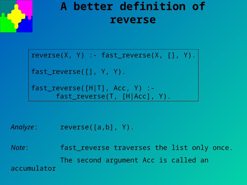
A better definition of reverse
reverse(X, Y) :- fast_reverse(X, [], Y).
fast_reverse([], Y, Y).
fast_reverse([H|T], Acc, Y) :- fast_reverse(T, [H|Acc], Y).
Note: fast_reverse traverses the list only once.
The second argument Acc is called an accumulator
Analyze: reverse([a,b], Y).

Execution of fast_reverse
reverse([a,b,c], Y) :- fast_reverse([a,b,c], [], Y).
fast_reverse ([a,b,c], [], Y) :- fast_reverse([b,c], [a], Y).
by rule 2
fast_reverse ([b,c], [a], Y) :- fast_reverse([c], [b,a], Y).
by rule 2
fast_reverse ([c], [b,a], Y) :- fast_reverse([], [c,b,a], Y).
by rule 1
fast_reverse ([], [c,b,a], [c,b,a])
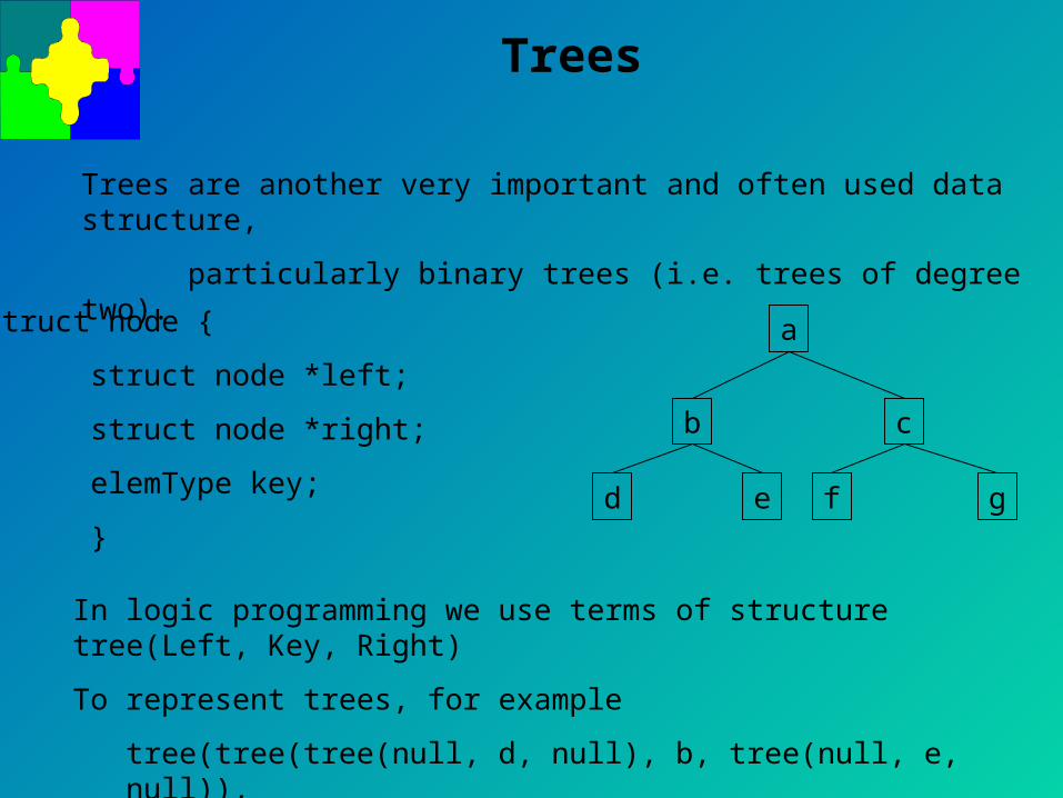
Trees
Trees are another very important and often used data structure,
particularly binary trees (i.e. trees of degree two).
astruct node {
struct node *left;
struct node *right;
elemType key;
}
b c
d e f g
In logic programming we use terms of structure tree(Left, Key, Right)
To represent trees, for example
tree(tree(tree(null, d, null), b, tree(null, e, null)),
tree(tree(null, f, null), c, tree(null, g, null)))
Tree Search
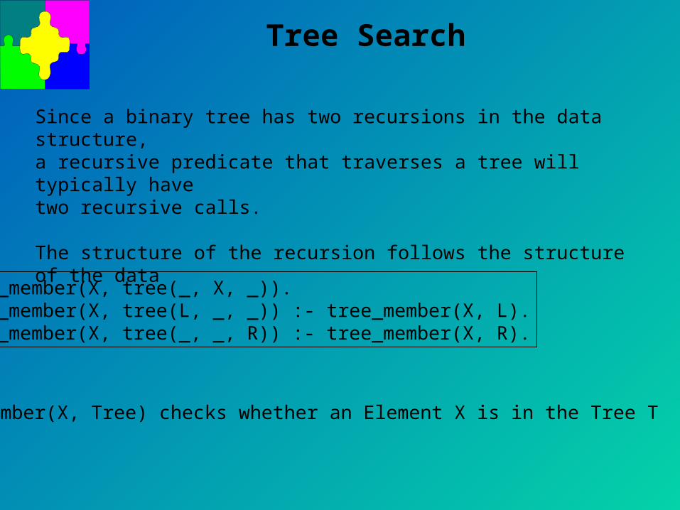
Since a binary tree has two recursions in the data structure, a recursive predicate that traverses a tree will typically havetwo recursive calls.
The structure of the recursion follows the structure of the data
tree_member(X, Tree) checks whether an Element X is in the Tree T
tree_member(X, tree(_, X, _)).tree_member(X, tree(L, _, _)) :- tree_member(X, L).tree_member(X, tree(_, _, R)) :- tree_member(X, R).

Tree Preorder Traversal
Tree traversals:
•Inorder: left child -> node -> right child
•Preorder: node -> left child -> right child
•Postorder: left child -> right child -> node
a
b c
d e f g
Preorder(null, []).Preorder(tree(L,X,R), [X | Rest]) :-
preorder(L, Left),preorder(R, Right),append(Left, Right, Rest).

Isomorphic Trees
Two binary Trees T1, T2 are called isomorphicIf T2 can be obtained from T1 by
swapping left and right subtrees.
a
b c
d e f g
a
c b
g f d e
isoTree(null, null).
isoTree(tree(L1, X, R1), tree(L2, X, R2)) :-isoTree(L1, L2), isoTree(R1, R2).
isoTree(tree(L1, X, R1), tree(L2, X, R2)) :-isoTree(L1, R2), isoTree(R1, L2).
iso

Impure Logic Programming: The Cut
Consider: member(X, [X|_]).member(X, [_|Rest]) :- member(X, Rest).
member finds duplicate solutions, e.g. member(a, [a,b,a,c,a,d]) suceeds three times.
What if we are only interested in a yes/no answer for member?=> We don’t want to consider the alternative solutions after the
first member is used.
A Cut (written as ‘!’) can be used to prune unwanted alternative solutionsthat could be found upon backtracking from the search tree.
member(X, [X|_]) :- !.member(X, [_|Rest]) :- member(X, Rest).
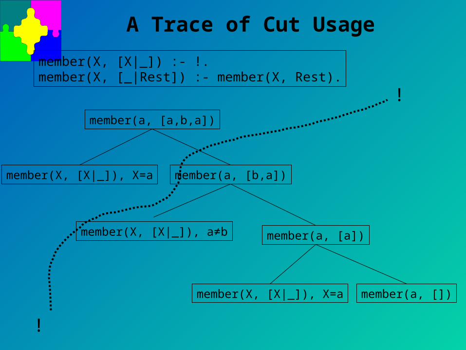
A Trace of Cut Usage
member(X, [X|_]) :- !.member(X, [_|Rest]) :- member(X, Rest).
member(a, [a,b,a])
member(X, [X|_]), X=a member(a, [b,a])
member(a, [a])
member(X, [X|_]), X=a
member(X, [X|_]), a≠b
member(a, [])
!
!

The Cut
•cuts of all subsequent rules for the predicate that follow the cut:
p(X) :- test(X), !, q(X).p(X) :- r(X).
r(X) will never be tried if test(X) succeeds.
•cuts of all alternative solutions for predicates left of the cut in this rule•it does not influence any predicates to its right.
p(X,Z) :- q(X,Y), !, r(Y,Z).
the definitions q(a,b). q(a,c). r(b,l). r(b,m). r(c,n)
will generate only the solutions p(a,l) and p(a,m), but not p(a,n).

Red Cuts
A typical usage of cuts is to avoid duplicate conditions in mutually exclusive tests.
Consider the following program:
minimum(X,Y,Z) :- X <= Y, Z=X.minimum(X,Y,Z) :- X > Y, Z=Y.
This can be rewritten as:
minimum(X,Y,Z) :- X <= Y, !, Z=X.minimum(X,Y,Z) :- Z=Y.
Be careful with such cuts, since removing them will change the meaning of the program. They are called “red cuts”.

NegationTo negate a test we write \+(G) (read as “not G”).
\+(G) is true if G is false, \+(G) is false, if G is true.
This can be used to negate conditions, for example:
minimum(X,Y,Z) :- \+(X>Y), Z=X.minimum(X,Y,Z) :- X>Y, Z=Y.
Procedurally Prolog executes \+(G) in the following way:G is executed. If G succeeds, the call to \+(G) fails.If G fails, the call to \+(G) succeeds.
This “Negation by failure” can be defined as:
not(G) :- G, !, fail.not(G).

Negation
Two things to keep in mind, when using negation:
•Negation never gives back any bindingsfor example: \+(edge(X,Y)) will never bind X or Y.
•Only the first successful execution of G is executed by the program