cse - iit kanpur

Bias/Variance Trade-off, Some Practical Issues,Semi-supervised and Active Learning

Piyush Rai

Introduction to Machine Learning (CS771A)

November 13, 2018

Intro to Machine Learning (CS771A) Bias/Variance Trade-off, Some Practical Issues, Semi-supervised and Active Learning 1

Plan for today

Bias/Variance Trade-off of Learning Algorithms

Some basic guidelines for debugging ML algorithms

What if training data and test data distributions are NOT the same

How to utilize unlabeled data: Semi-supervised Learning

How to selectively ask for the most informative data: Active Learning


Bias/Variance Trade-off


A Fundamental Decomposition

Assume F to be a class of models (e.g., set of linear classifiers with some pre-defined features)

Suppose we’ve learned a model f ∈ F learned using some (finite amount of) training data

Can decompose the test error ε(f ) of f as follows

ε(f ) =

[minf ∗∈F

ε(f ∗)

]︸︷︷︸

approximation error

+

[ε(f )− min

f ∗∈Fε(f ∗)

]︸︷︷︸

estimation error

Here f ∗ is the best possible model in F assuming infinite amount of training data

Approximation error: Error of best model f ∗ because of the model class F being too simple

Estimation error: Error of learned model f (relative to f ∗) because we only had finite training data


A Trade-off

There is a trade-off between the two components of the error

ε(f ) =

[minf ∗∈F

ε(f ∗)

]︸︷︷︸approximation error

+

[ε(f )− min

f ∗∈Fε(f ∗)

]︸︷︷︸

estimation error

Can reduce the approximation error by making F more complex/richer, e.g.,

Replace the linear classifiers by a higher order polynomials

Add more features in the data

However, making F richer will usually cause estimation error to increase since f can now overfit

f may give small error on some datasets, large error on some datasets

Note: The above trade-off is popularly known as the bias/variance trade-off

Approximation error known as “bias”(high if the model is simple)

Estimation error known as “variance”(high if the model is complex)


A Visual Illustration of the Trade-off

Model Complexity

BiasVariance

Test Error

Small Medium High

Underfitting Overfitting

Training Error


Debugging ML Algorithms


Debugging Learning Algorithms

A notoriously hard problem in general

Note that code for ML algorithms is not procedural but data-driven

What to do when our model (say logistic regression) isn’t doing well on test data

Use more training examples to train the model?

Use a smaller number of features?

Introduce new features (can be combinations of existing features)?

Try tuning the regularization parameter?

Run (the iterative) optimizer longer, i.e., for more iterations?

Change the optimization algorithm (e.g., GD to SGD or Newton..)?

Give up and switch to a different model (e.g., SVM)?

How to know what might be going wrong and how to debug?


High Bias or High Variance?

The bad performance (low accuracy on test data) could be due either

High Bias (Underfitting)

High Variance (Overfitting)

Looking at the training and test error can tell which of the two is the case

Model Complexity

BiasVariance

Test Error

Small Medium High


Training Error

High Bias: Both training and test errors are large

High Variance: Small training error, large test error (and huge gap)


Some Guidelines for Debugging Learning Algorithms

Model Complexity

BiasVariance

Test Error

Small Medium High


Training Error

If the model has high bias (underfitting) then the model class is weak

Adding more training data won’t help

Instead, try making the model class richer, or add more features (makes the model richer)

If the model has high variance (overfitting) then the model class is sufficiently rich

Adding more training data can help (overfitting might be due to limited training data)

Using a simpler model class or fewer features or regularization can help


When Train and Test Distributions Differ


When Train and Test Conditions are Different..

Training and test inputs typically assumed to be drawn from same distribution, i.e., ptr (x) = pte(x)

However, this is rarely true in real-world applications of ML where ptr (x) 6= pte(x)

So the training and test data are from different “domains”. How can we “adapt”?

Known as “domain adaptation” (also “covariate-shift”, since features x are also called covariates)


Handling Domain Differences: Some Approaches

Learning a transformation that makes the training and test data distributions “close”

Use an “importance weighted” correction of the loss function defined on the training data

N∑n=1

pte(xn)

ptr (xn)`(yn, f (xn))

.. basically, assign a weight to each term of the loss function, depending on how “close” the trainingexample (xn, yn) is from the test distribution


Importance-Weighted Correction: A Closer Look

Note that, since we care about test data, ideally, we would like to learn f by minimizing

Epte(x)[`(y , f (x))] =

∫pte(x)`(y , f (x))dx

However, we don’t have labeled data from the test domain. :-( What can we do now?

Let’s re-express the above in terms of the loss on training data∫pte(x)`(y , f (x))dx =

∫ptr (x)

pte(x)

ptr (x)`(y , f (x))dx

= Eptr (x)

[pte(x)

ptr (x)`(y , f (x))

]≈

N∑n=1

pte(xn)

ptr (xn)`(yn, f (xn)) (uses only training data from ptr )

In order to do this, we need to estimate the two densities ptr (x) and pte(x) (can assume some formfor these and estimate them using unlabeled data from both domains)


Semi-supervised Learning


Labeled vs Unlabeled Data

Supervised Learning models require labeled data

Learning a reliable model usually requires plenty of labeled data

Labeled Data: Expensive and Scarce (someone has to do the labeling)

Often labeling is very difficult too (e.g., in speech analysis or NLP problems)

Unlabeled Data: Abundant and Free/Cheap

E.g., can easily crawl the web and download webpages/images


Learning with Labeled+Unlabeled Data

Usually such problems come in one of the following two flavors

Semi-supervised Learning

Training set containslabeled data L = {x i , yi}Li=1 and unlabeled data U = {x j}L+Uj=L+1 (usually U � L)

Note: In some cases, U is also our test data (this is called transductive setting)

Inductive setting is more standard: Want to learn a classifier for future test data

Semi-Unsupervised Learning

We are given unlabeled data D = {x i}Ni=1

Additionally, we’re given supervision in form of some constraints on data (e.g., points xn and xm

belong to the same cluster) or “labels” of some points.

Want to learn an unsupervised learning model combining both data sources

Here, we will focus on Semi-supervised Learning (SSL)


Why/How Might Unlabeled Data Help?

Red: + 1, Dark Blue: -1

Let’s include some additional unlabeled points (Light Blue points)

Assumption: Examples from the same class are clustered together

Assumption: Decision boundary lies in the region where data has low density


Why/How Might Unlabeled Data Help?

Knowledge of the input distribution helps even if the data is unlabeled


Some Basic Assumptions used in SSL

Nearby points (may) have the same label

Smoothness assumption

Points in the same cluster (may) have same label

Cluster assumption

Decision boundary lies in areas where data has low density

Low-density separation

Note: Generative models already take some of these assumptions into account (recall HW3problem on semi-supervised learning using EM)


SSL using Graph-based Regularization

Based on smoothness assumption

Requires constructing a graph between all the examples (labeled/unlabeled)

The graph can be constructed using several ways

Connecting every example with its top k neighbors (labeled/unlabeled)

Constructing an all-connected weighted graph

Weighted case: weight of edge connecting examples x i and x j

aij = exp(−||x i − x j ||2/σ2)

.. where A is the (L + U)× (L + U) matrix of pairwise similarities


SSL using Graph-based Regularization

Suppose we want to learn a function f using labeled+unlabeld data L ∪ U

Suppose fi denotes the prediction on example x i

Similar examples x i and x j (thus high aij) should have similar fi and fj

Graph-based regularization optimizes the following objective:

minf

∑i∈L

`(yi , fi )︸︷︷︸loss term

+ λR(f )︸︷︷︸usual regularizer

+ γ∑

i,j∈L,U

aij(fi − fj)2

︸︷︷︸graph-based regularizer


SSL using EM based Generative Classification

Suppose data D is labeled L = {x i , yi}Li=1 and unlabeled U = {x j}L+Uj=L+1

Assume the following model

p(D|θ) =L∏

i=1

p(x i , yi |θ)

︸︷︷︸labeled

L+U∏j=L+1

p(x j |θ)

︸︷︷︸unlabeled

=L∏

i=1

p(x i , yi |θ)L+U∏j=L+1

∑yj

p(x j , yj |θ)

The unknowns are {yj}L+Uj=L+1 (latent variables) and θ (parameters)

We can use EM to estimate the unknowns

Given θ = θ̂, E step will compute expected labels for unlabeled examples

E[yj ] = +1× P(yj = +1|θ̂, x j) + (−1)× P(yj = −1|θ̂, x j)

M step can then perform standard MLE for re-estimating the parameters θ

A fairly general framework for semi-supervised learning. Can be used for different types of data (bychoosing the appropriate p(x |y) distribution)


Things can go wrong..

If assumptions are not appropriate for the data (e.g., incorrectly specified class conditional distributions)

Thus need to be careful/flexible about the choice of class conditional distributions


Active Learning


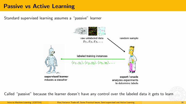
Passive vs Active Learning

Standard supervised learning assumes a “passive” learner

Called “passive” because the learner doesn’t have any control over the labeled data it gets to learn


Active Learning

An “active” learner can specifically request labels of “hard” examples that are most useful for learning

How to quantify the “hardness” or “usefulness” of an unlabeled example?


Active Learning

Various ways to define the usefulness/hardness of an unlabeled example x

A probabilistic approach can use distribution of y given x to quantify usefulness of x , e.g.,

In classification, can look at the entropy of the distribution p(y |x ,w) or posterior predictive p(y |x)

.. and choose example(s) for which the distribution of y given x has the largest entropy

Look at the variance of the posterior predictive p(y |x). E.g. for regression,

.. and choose choose example(s) for which variance of posterior predictive is the largest

.. many other ways to utilize the information in p(y |x)


cse - iit kanpur

Documents