cse 774 robotic systemsyiannisr/774/2014/lectures/06-pathplanning.pdf · call the line from the...
TRANSCRIPT

Ioannis Rekleitis
Path Planning

Outline
• Path Planning
– Visibility Graph
– Potential Fields
– Bug Algorithms
– Skeletons/Voronoi Graphs
– C-Space
2CSCE-774 Robotic Systems
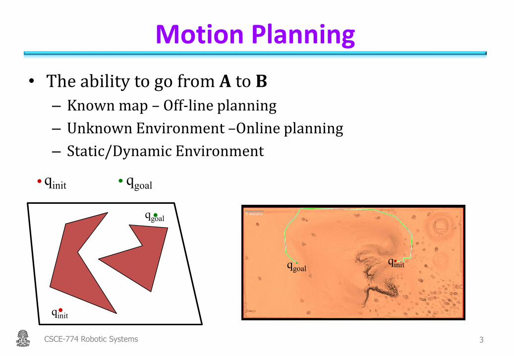
Motion Planning
• The ability to go from A to B
– Known map – Off-line planning
– Unknown Environment –Online planning
– Static/Dynamic Environment
CSCE-774 Robotic Systems 3
qgoalqinit
qgoal
qgoalqinit
qinit
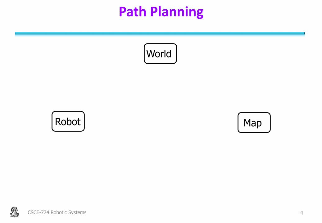
Path Planning
Robot Map
World
4CSCE-774 Robotic Systems
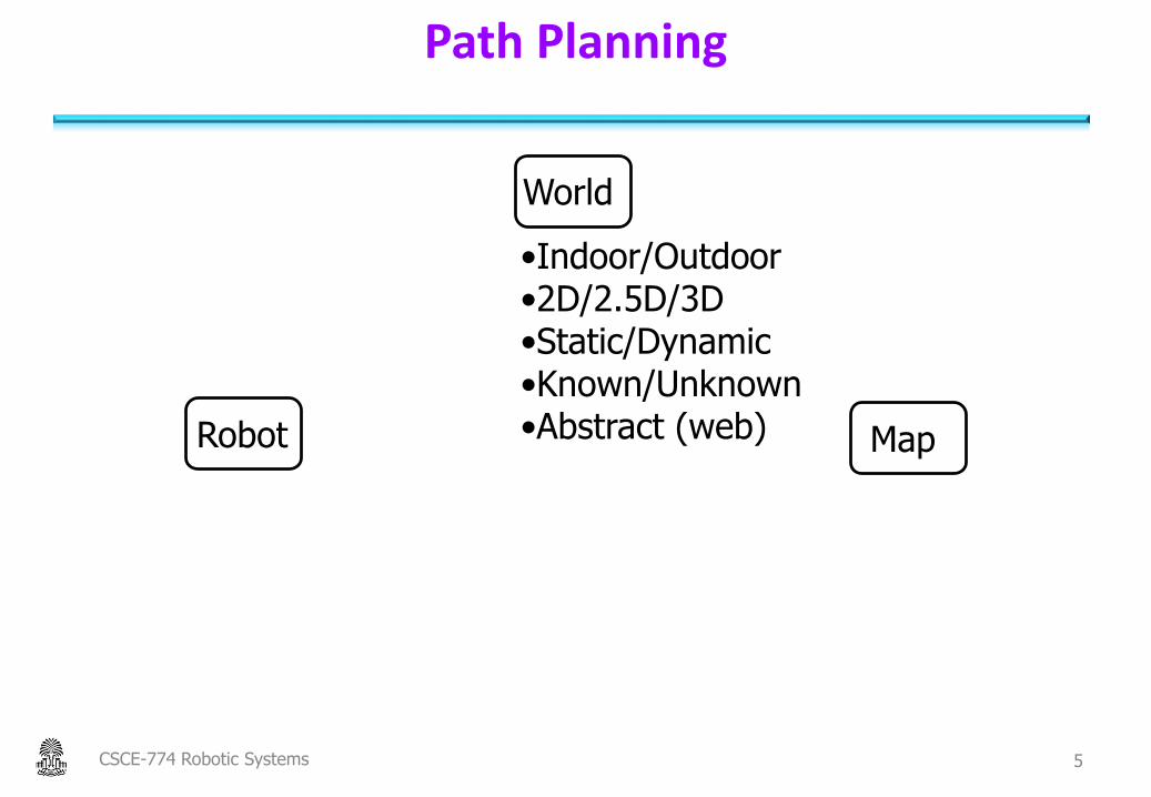
Path Planning
Robot Map
World
•Indoor/Outdoor•2D/2.5D/3D•Static/Dynamic•Known/Unknown•Abstract (web)
5CSCE-774 Robotic Systems
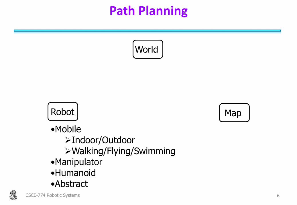
Path Planning
Robot Map
World
•MobileIndoor/OutdoorWalking/Flying/Swimming
•Manipulator•Humanoid•Abstract
6CSCE-774 Robotic Systems
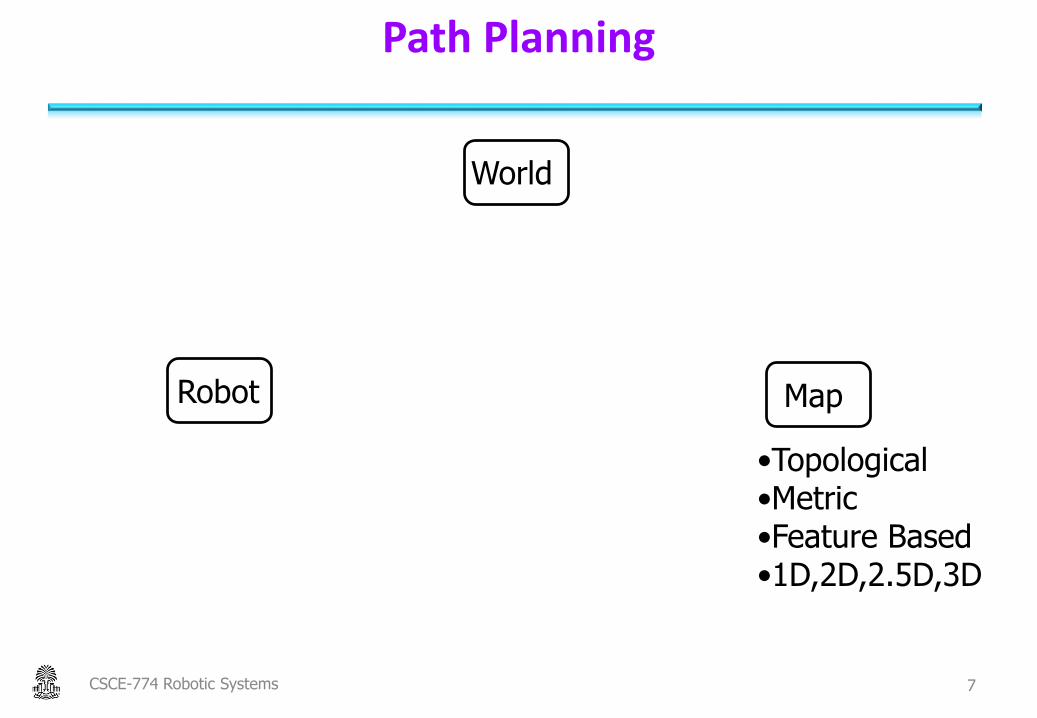
Path Planning
Robot Map
World
•Topological•Metric•Feature Based•1D,2D,2.5D,3D
7CSCE-774 Robotic Systems

Path Planning
Robot Map
World
•Topological•Metric•Feature Based•1D,2D,2.5D,3D
•MobileIndoor/OutdoorWalking/Flying/Swimming
•Manipulator•Humanoid•Abstract
•Indoor/Outdoor•2D/2.5D/3D•Static/Dynamic•Known/Unknown•Abstract (web)
8CSCE-774 Robotic Systems

Path Planning: Assumptions
• Known Map
• Roadmaps (Graph representations)
• Polygonal Representation
qgoal
qinit
9CSCE-774 Robotic Systems

Visibility Graph
• Connect Initial and goal locations with all the visible vertices
qgoal
qinit
10CSCE-774 Robotic Systems
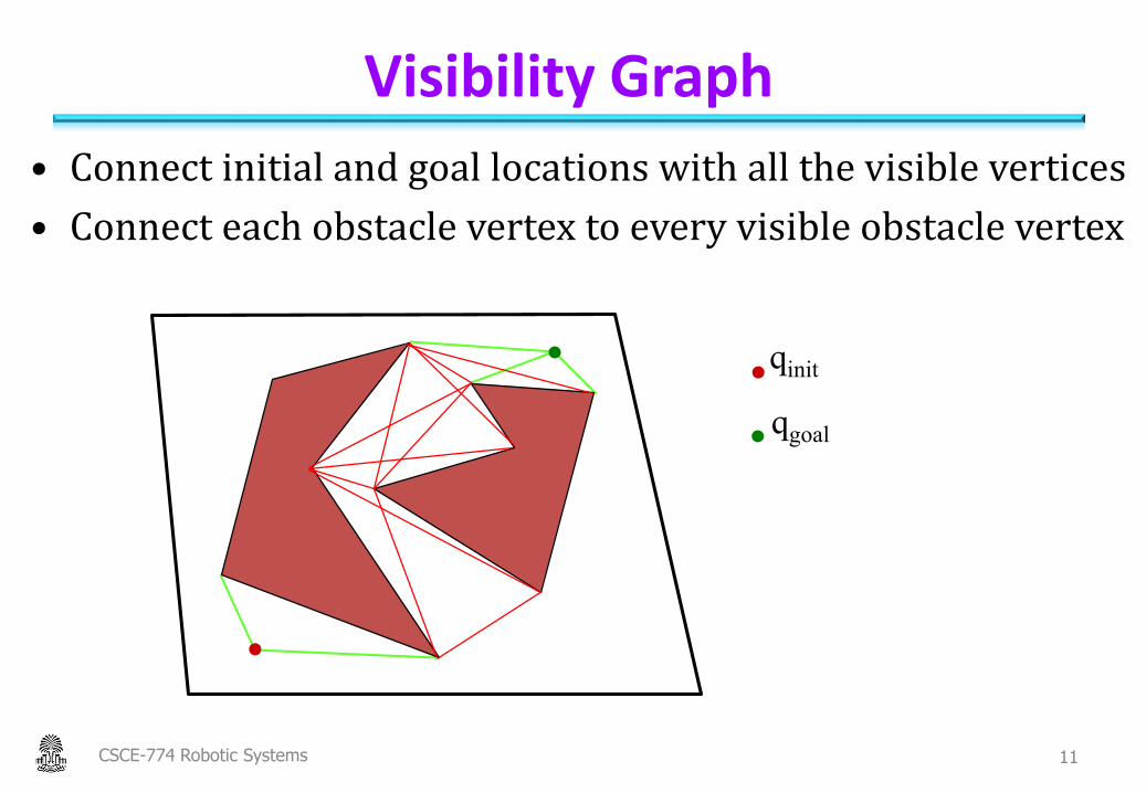
Visibility Graph
• Connect initial and goal locations with all the visible vertices
• Connect each obstacle vertex to every visible obstacle vertex
qgoal
qinit
11CSCE-774 Robotic Systems

Visibility Graph
• Connect initial and goal locations with all the visible vertices
• Connect each obstacle vertex to every visible obstacle vertex
• Remove edges that intersect the interior of an obstacle
qgoal
qinit
12CSCE-774 Robotic Systems

Visibility Graph• Connect initial and goal locations with all the visible vertices
• Connect each obstacle vertex to every visible obstacle vertex
• Remove edges that intersect the interior of an obstacle
• Plan on the resulting graph
qgoal
qinit
13CSCE-774 Robotic Systems

Visibility Graph• An alternative path
• Alternative name: “Rubber band algorithm”
qgoal
qinit
14CSCE-774 Robotic Systems

Major Fault• Point robot
• Path planning like that guarantees to hit the obstacles
15CSCE-774 Robotic Systems
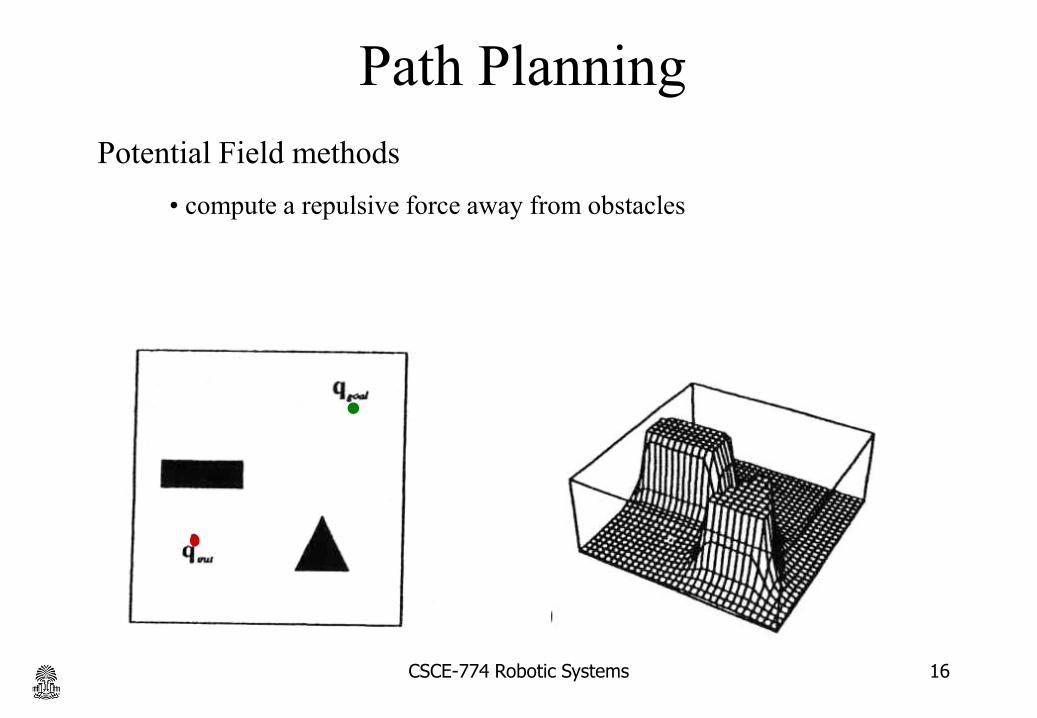
Path Planning
Potential Field methods
• compute a repulsive force away from obstacles
CSCE-774 Robotic Systems 16

Local techniques
Potential Field methods
• compute a repulsive force away from obstacles
• compute an attractive force toward the goal
CSCE-774 Robotic Systems 17

Local techniques
Potential Field methods
• compute a repulsive force away from obstacles
• compute an attractive force toward the goal
let the sum of the forces control the robot
key advantages?CSCE-774 Robotic Systems 18

Local techniques
Potential Field methods
• compute a repulsive force away from obstacles
• compute an attractive force toward the goal
let the sum of the forces control the robot
To a large extent, this is
computable from sensor readingsCSCE-774 Robotic Systems 19
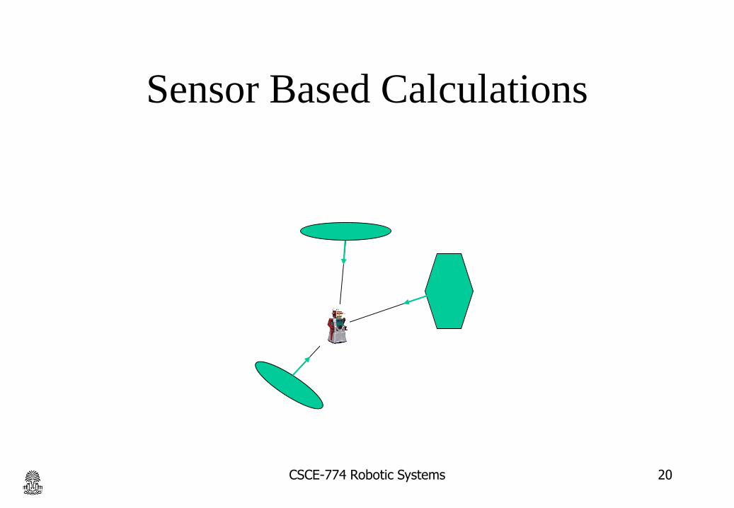
Sensor Based Calculations
CSCE-774 Robotic Systems 20

Major Problem?
CSCE-774 Robotic Systems 21
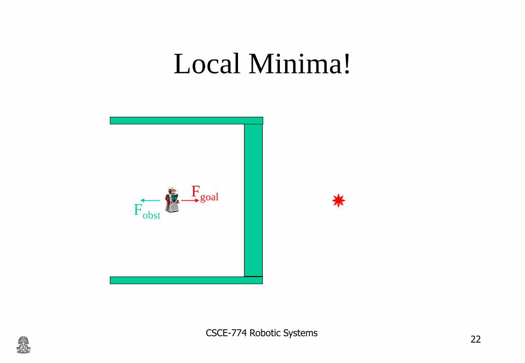
Local Minima!
Fobst
Fgoal
CSCE-774 Robotic Systems22
Simulated Annealing
• Every so often add some random force
CSCE-774 Robotic Systems 23
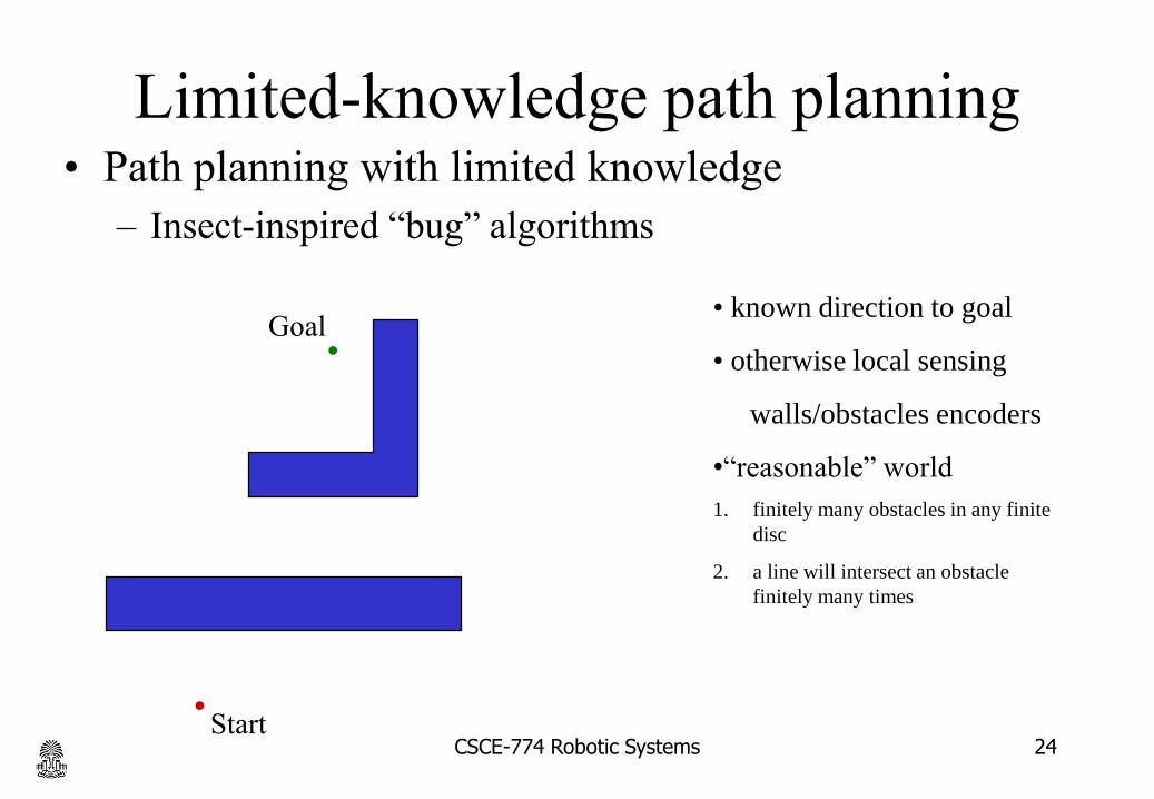
Limited-knowledge path planning
• known direction to goal
• otherwise local sensing
walls/obstacles encoders
•“reasonable” world
1. finitely many obstacles in any finite
disc
2. a line will intersect an obstacle
finitely many times
Goal
Start
• Path planning with limited knowledge
– Insect-inspired “bug” algorithms
24CSCE-774 Robotic Systems
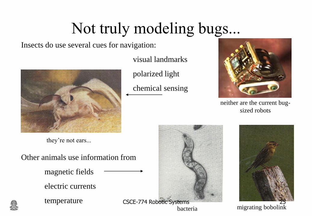
Not truly modeling bugs...Insects do use several cues for navigation:
neither are the current bug-
sized robots
visual landmarks
polarized light
chemical sensing
Other animals use information from
magnetic fields
electric currents
temperature
they’re not ears...
migrating bobolinkbacteria25CSCE-774 Robotic Systems

Bug Strategy
“Bug 0” algorithm
• known direction to goal
• otherwise only local sensing
walls/obstacles encoders
1) head toward goal
2) follow obstacles until you can
head toward the goal again
3) continue
Insect-inspired “bug” algorithms
CSCE-774 Robotic Systems 26
assume a
left-turn robot
Does It Work?
27CSCE-774 Robotic Systems
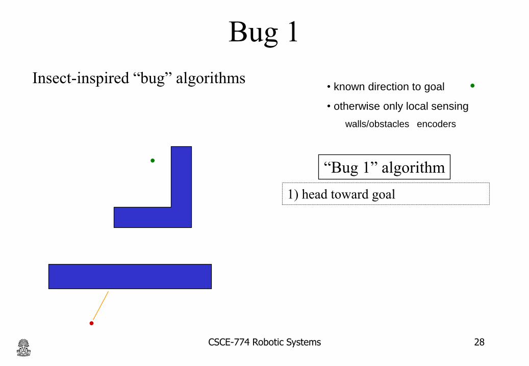
“Bug 1” algorithm
• known direction to goal
• otherwise only local sensing
walls/obstacles encoders
1) head toward goal
Insect-inspired “bug” algorithms
Bug 1
CSCE-774 Robotic Systems 28
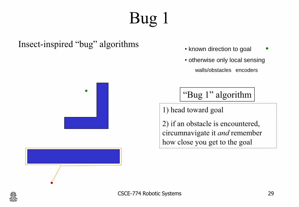
“Bug 1” algorithm
• known direction to goal
• otherwise only local sensing
walls/obstacles encoders
1) head toward goal
2) if an obstacle is encountered,
circumnavigate it and remember
how close you get to the goal
Insect-inspired “bug” algorithms
Bug 1
CSCE-774 Robotic Systems 29

“Bug 1” algorithm
• known direction to goal
• otherwise only local sensing
walls/obstacles encoders
1) head toward goal
2) if an obstacle is encountered,
circumnavigate it and remember
how close you get to the goal
3) return to that closest point (by
wall-following) and continue
Insect-inspired “bug” algorithms
Vladimir Lumelsky & Alexander Stepanov Algorithmica 1987
Bug 1
CSCE-774 Robotic Systems 30
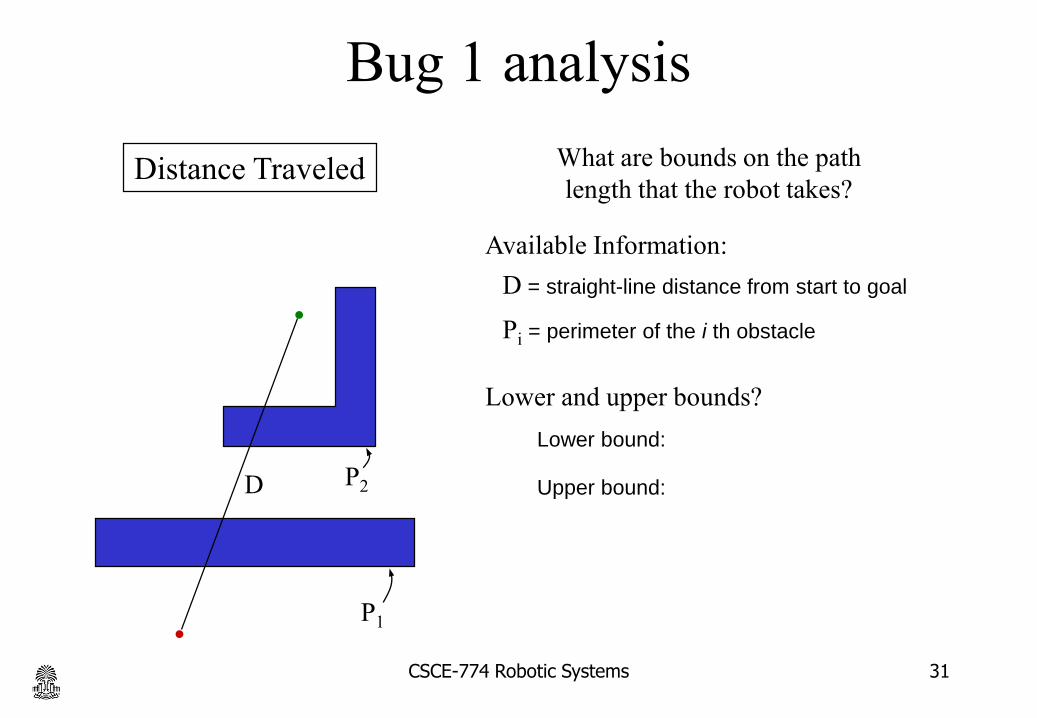
Distance Traveled What are bounds on the path
length that the robot takes?
Lower and upper bounds?
Available Information:
D = straight-line distance from start to goal
Pi = perimeter of the i th obstacle
Lower bound:
Upper bound:
Bug 1 analysis
CSCE-774 Robotic Systems 31
D
P1
P2

Distance Traveled What are bounds on the path
length that the robot takes?
Lower and upper bounds?
Available Information:
D = straight-line distance from start to goal
Pi = perimeter of the i th obstacle
Lower bound: D
Upper bound:
Bug 1 analysis
CSCE-774 Robotic Systems 32
D
P1
P2

Distance Traveled What are bounds on the path
length that the robot takes?
Lower and upper bounds?
Available Information:
D = straight-line distance from start to goal
Pi = perimeter of the i th obstacle
Lower bound: D
Upper bound: D + 1.5 Pii
How good a bound?
How good an algorithm?
Bug 1 analysis
CSCE-774 Robotic Systems 33
D
P1
P2
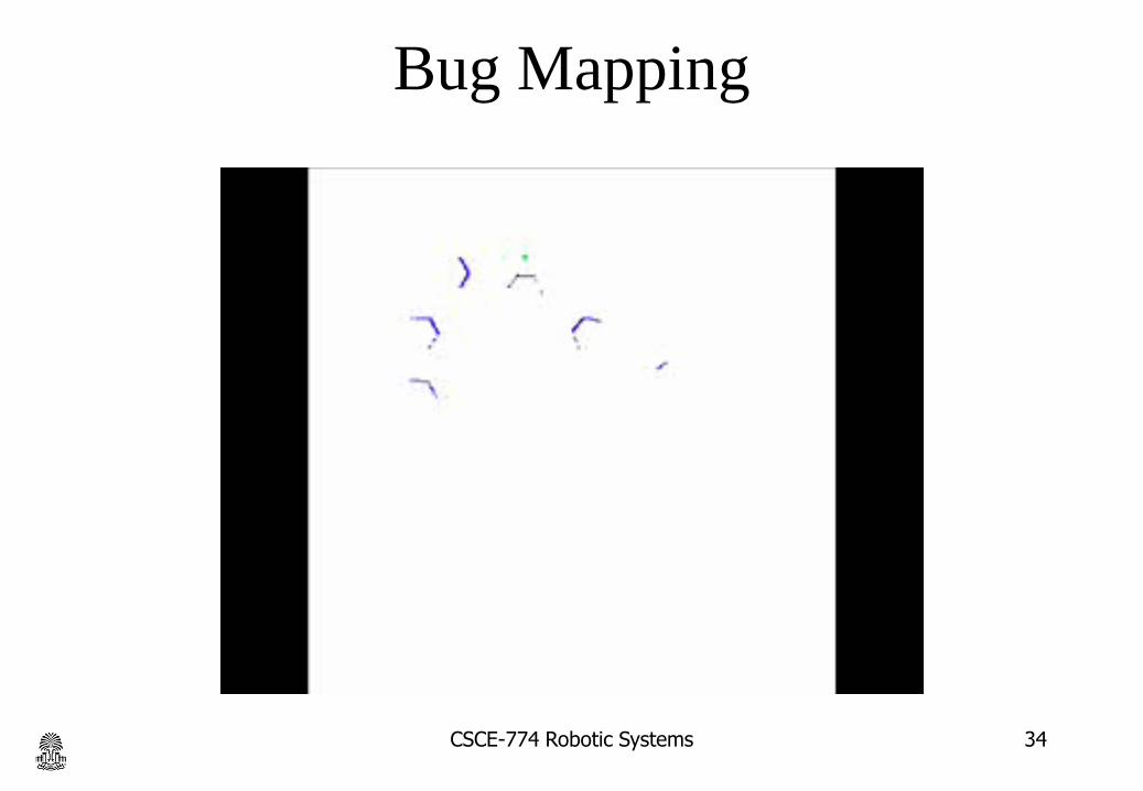
Bug Mapping
34CSCE-774 Robotic Systems

“Bug 2” algorithmCall the line from the starting
point to the goal the s-line
A better bug?
CSCE-774 Robotic Systems 35
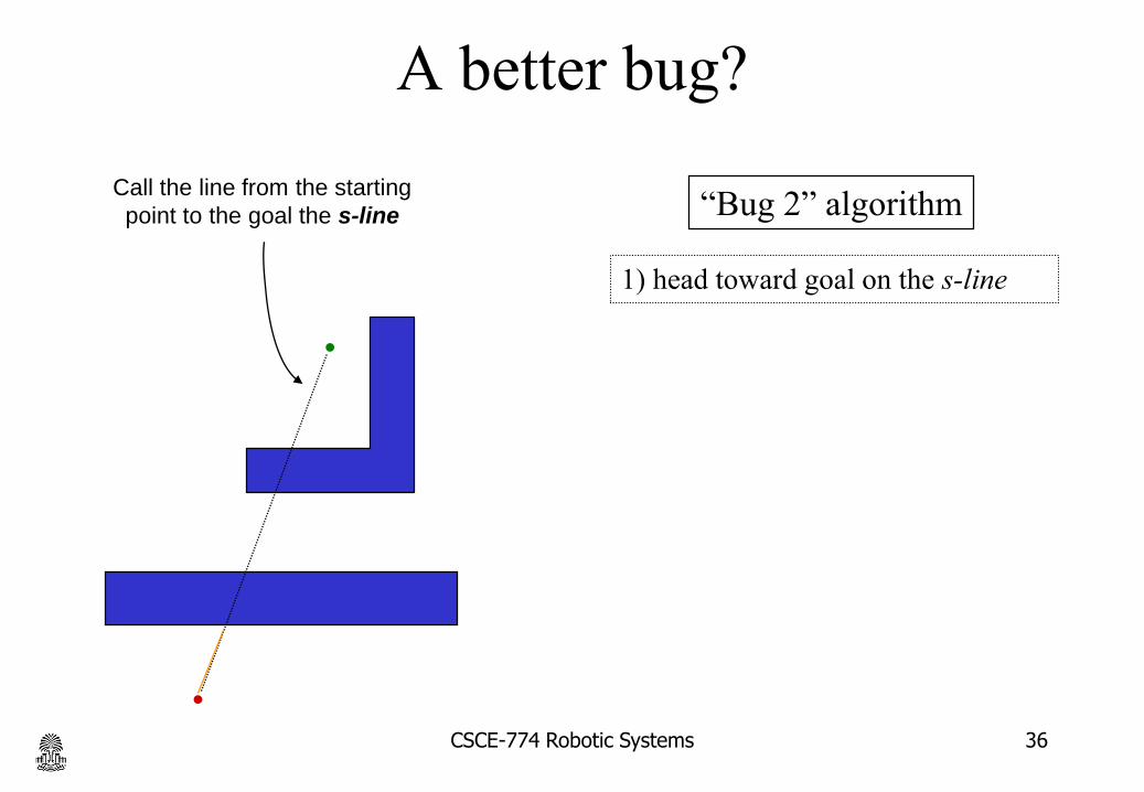
“Bug 2” algorithmCall the line from the starting
point to the goal the s-line
1) head toward goal on the s-line
A better bug?
CSCE-774 Robotic Systems 36

“Bug 2” algorithmCall the line from the starting
point to the goal the s-line
1) head toward goal on the s-line
2) if an obstacle is in the way,
follow it until encountering the s-
line again.
A better bug?
CSCE-774 Robotic Systems 37

“Bug 2” algorithm
1) head toward goal on the s-line
2) if an obstacle is in the way,
follow it until encountering the s-
line again.
3) Leave the obstacle and continue
toward the goal
OK ?
s-line
A better bug?
CSCE-774 Robotic Systems 38
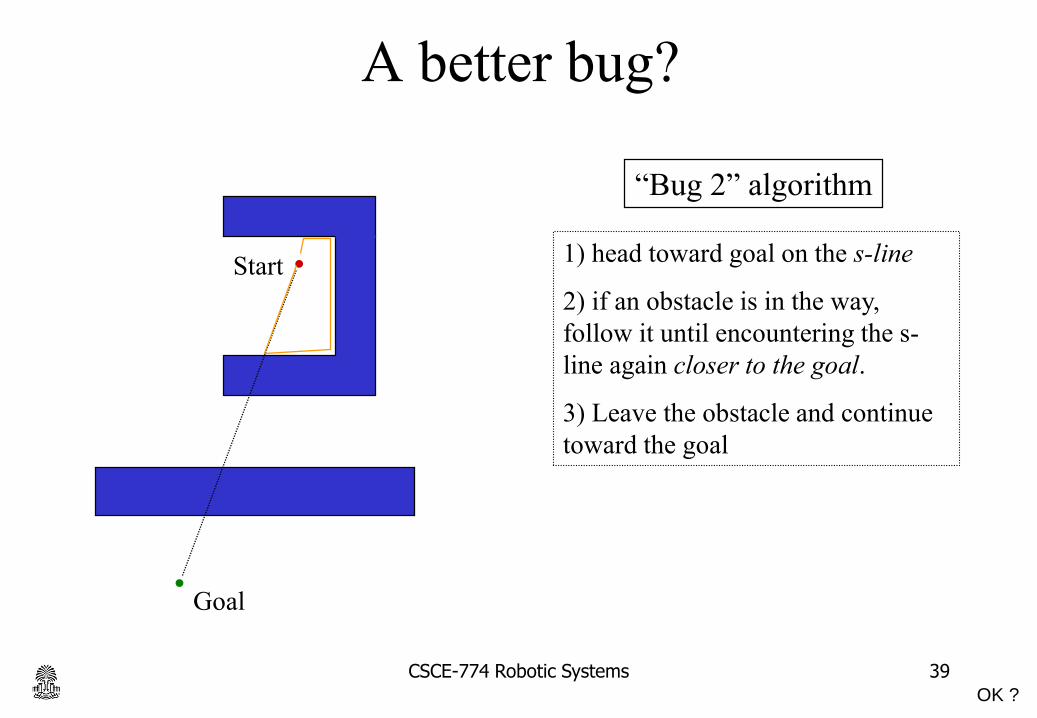
“Bug 2” algorithm
1) head toward goal on the s-line
2) if an obstacle is in the way,
follow it until encountering the s-
line again closer to the goal.
3) Leave the obstacle and continue
toward the goal
OK ?
A better bug?
CSCE-774 Robotic Systems 39
Goal
Start

Distance Traveled What are bounds on the path
length that the robot takes?
Lower and upper bounds?
Available Information:
D = straight-line distance from start to goal
Pi = perimeter of the i th obstacle
Lower bound:
Upper bound:
Bug 2 analysis
CSCE-774 Robotic Systems 40
Goal
Start

Distance Traveled What are bounds on the path
length that the robot takes?
Lower and upper bounds?
Available Information:
D = straight-line distance from start to goal
Pi = perimeter of the i th obstacle
Lower bound:
Upper bound:
Ni = number of s-line intersections
with the i th obstacle
Bug 2 analysis
CSCE-774 Robotic Systems 41
Goal
Start

Distance Traveled What are bounds on the path
length that the robot takes?
Lower and upper bounds?
Available Information:
D = straight-line distance from start to goal
Pi = perimeter of the i th obstacle
Lower bound: D
Upper bound:
Ni = number of s-line intersections
with the i th obstacle
Bug 2 analysis
CSCE-774 Robotic Systems 42
Goal
Start

Distance Traveled What are bounds on the path
length that the robot takes?
Lower and upper bounds?
Available Information:
D = straight-line distance from start to goal
Pi = perimeter of the i th obstacle
Lower bound: D
Upper bound: D + 0.5 Ni Pi
Ni = number of s-line intersections
with the i th obstacle
i
Bug 2 analysis
CSCE-774 Robotic Systems 43
Goal
Start

head-to-head comparison
What are worlds in which Bug 2 does
better than Bug 1 (and vice versa) ?
Bug 2 beats Bug 1
or thorax-to-thorax, perhaps
Bug 1 beats Bug 2
CSCE-774 Robotic Systems 44

head-to-head comparison
What are worlds in which Bug 2 does
better than Bug 1 (and vice versa) ?
Bug 2 beats Bug 1
or thorax-to-thorax, perhaps
Bug 1 beats Bug 2
CSCE-774 Robotic Systems 45
“zipper world”
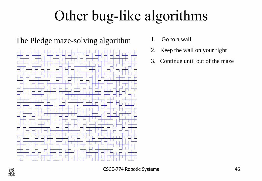
Other bug-like algorithms
The Pledge maze-solving algorithm 1. Go to a wall
2. Keep the wall on your right
3. Continue until out of the maze
46CSCE-774 Robotic Systems

Other bug-like algorithms
The Pledge maze-solving algorithm 1) Go to a wall
2) Keep the wall on your right
3) Continue until out of the maze
mazes of unusual origin
int a[1817];main(z,p,q,r){for(p=80;q+p-80;p=2*a[p])
for(z=9;z--;)q=3&(r=time(0)+r*57)/7,q=q?q-1?q-2?1-p%79?-
1:0:p%79-77?1:0:p<1659?79:0:p>158?-
79:0,q?!a[p+q*2]?a[p+=a[p+=q]=q]=q:0:0;for(;q++-
1817;)printf(q%79?"%c":"%c\n"," #"[!a[q-1]]);}
###############################################################################
# # ### # # # # # # # # # # # # # #
# # ####### ##### ##### # ####### # # ### ### # ##### ##### # ### ##### # ### #
# # # # # # # # # # # # # # # # # # # #
# ##### # # # # # # ##### ##### # ### ### # # # ### ### ### ##### # ### ##### #
# # # # # # # # # # # # # # # #
# # ### ##### ### ##### ##### ### # ### # # # # ### ##### ### ##### # ##### ###
# # # # # # # # # # # # # # # # # # # # # #
######### ##### # # # ########### ### ########### ### ##### ##### # # # ### # #
# # # # # # # # # # # # # # # # # # # # # #
### ### ##### ####### ### # # ### # # # # ##### # # ##### # # # ### # # ##### #
# # # # # # # # # # ### # # # # # # # # #
### # ### # ##### ### # ##### # # # ##### ##### ### ### ####### # ##### # ### #
# # # # # # # # # # # # # # # # # # # # # # #
# # # ########### ### ### ### ####### # # ### # ####### ### ##### ### ### #####
# # # # # # # # # # # # # # # #
# # # ### ##### ##### # ####### # ### ####### ### # ### ####### ### ##### ### #
# # # # # # # # # # # # # # # # # # # # #
# # # ### ### ### # # # # ### # # # ### # ####### # # ####### # # # # # # ### #
# # # # # # # # # # # # # # # # # #
# # # # # ### ##### ####### # ##### # ##### ### ### # # # ### ##### ### # ### #
# # # # # # # ### # # # # # # # # # # # # #
###############################################################################
IOCCC random maze generator
discretized RRT 47CSCE-774 Robotic Systems
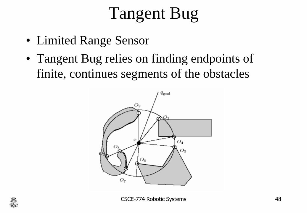
Tangent Bug
• Limited Range Sensor
• Tangent Bug relies on finding endpoints of
finite, continues segments of the obstacles
48CSCE-774 Robotic Systems
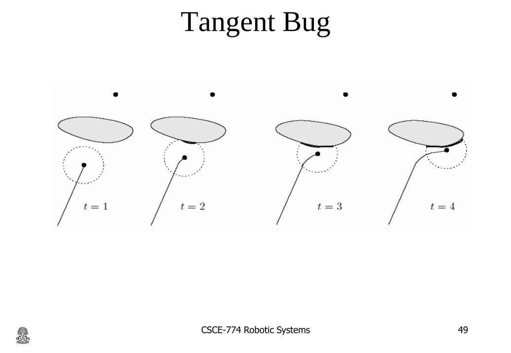
Tangent Bug
49CSCE-774 Robotic Systems

Contact Sensor Tangent Bug
1. Robot moves toward goal until it hits obstacle 1 at H12. Pretend there is an infinitely small sensor range and the direction which
minimizes the heuristic is to the right3. Keep following obstacle until robot can go toward obstacle again4. Same situation with second obstacle5. At third obstacle, the robot turned left until it could not increase heuristic6. D_followed is distance between M3 and goal, d_reach is distance between
robot and goal because sensing distance is zero50CSCE-774 Robotic Systems
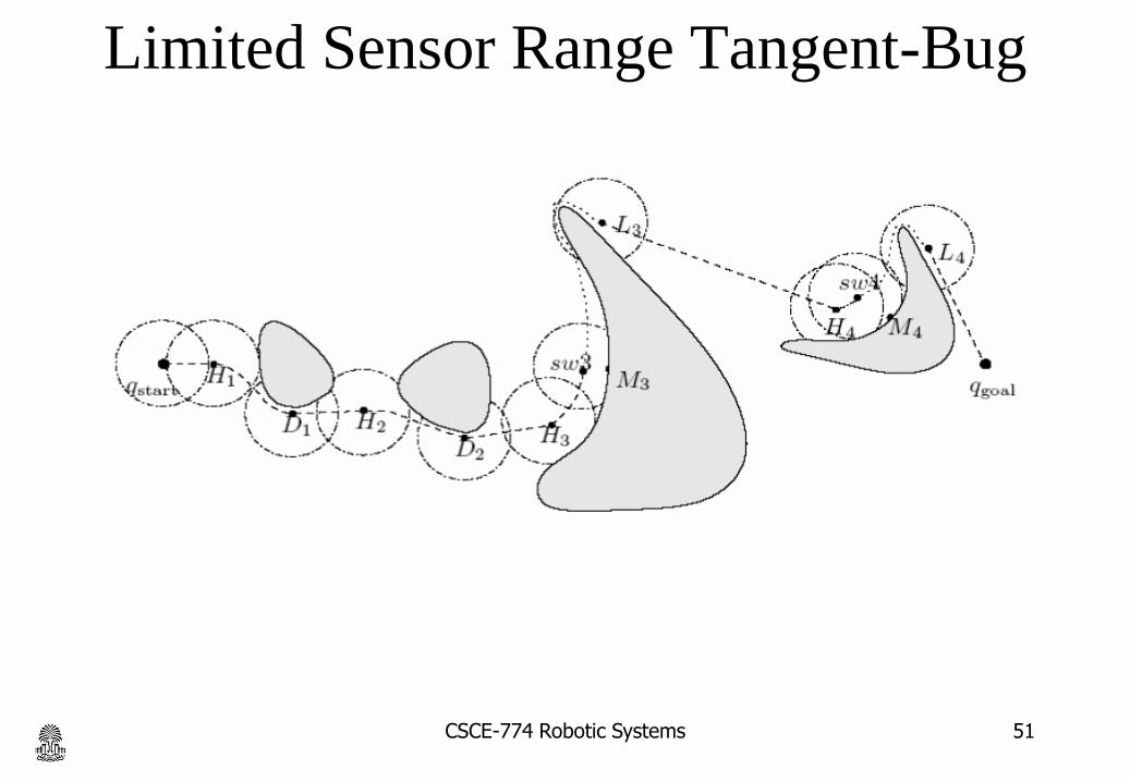
Limited Sensor Range Tangent-Bug
51CSCE-774 Robotic Systems
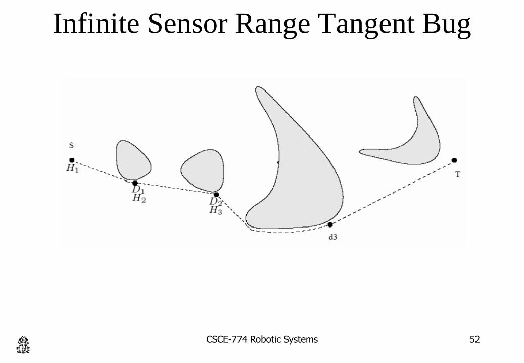
Infinite Sensor Range Tangent Bug
52CSCE-774 Robotic Systems
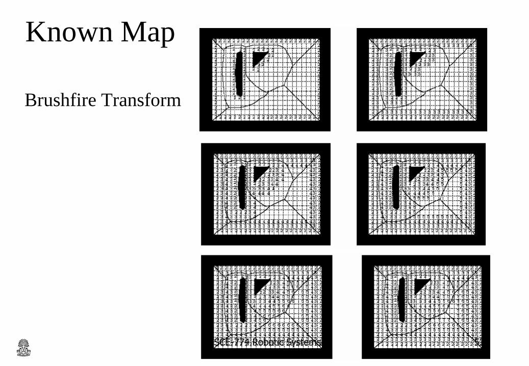
Known Map
Brushfire Transform
CSCE-774 Robotic Systems 53
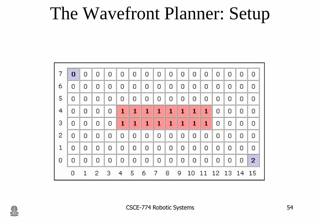
The Wavefront Planner: Setup
CSCE-774 Robotic Systems 54

The Wavefront in Action (Part 1)
• Starting with the goal, set all adjacent cells with “0” to the
current cell + 1
– 4-Point Connectivity or 8-Point Connectivity?
– Your Choice. We’ll use 8-Point Connectivity in our example
CSCE-774 Robotic Systems 55

The Wavefront in Action (Part 2)• Now repeat with the modified cells
– This will be repeated until no 0’s are adjacent to cells with values >= 2
• 0’s will only remain when regions are unreachable
CSCE-774 Robotic Systems 56

The Wavefront in Action (Part 3)• Repeat
CSCE-774 Robotic Systems 57
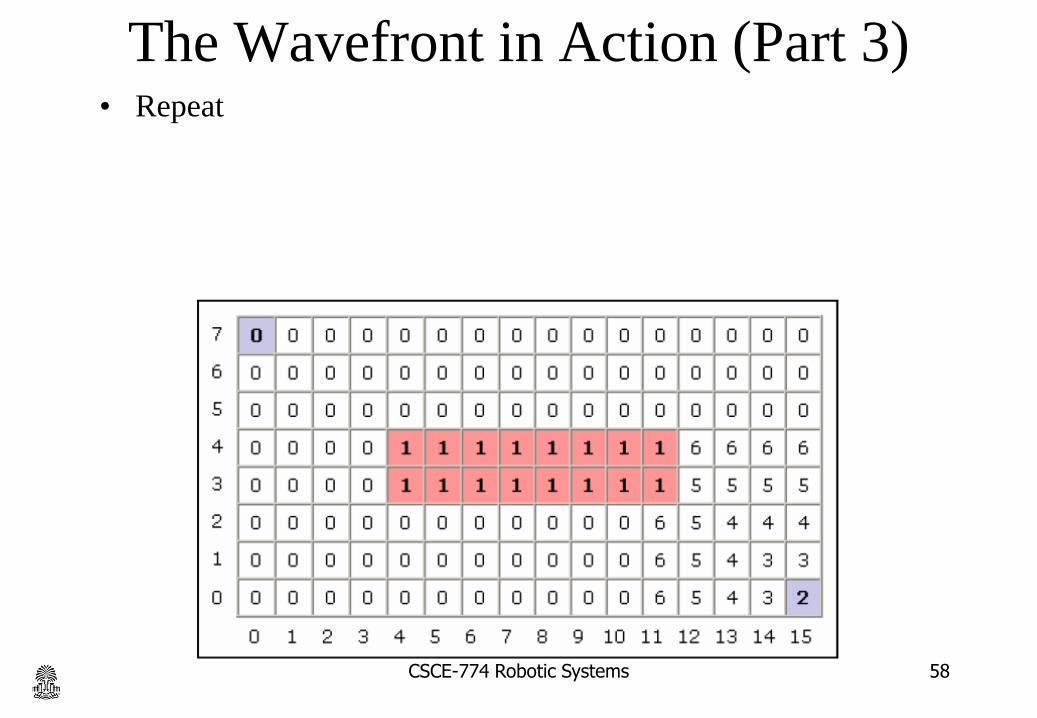
The Wavefront in Action (Part 3)• Repeat
CSCE-774 Robotic Systems 58
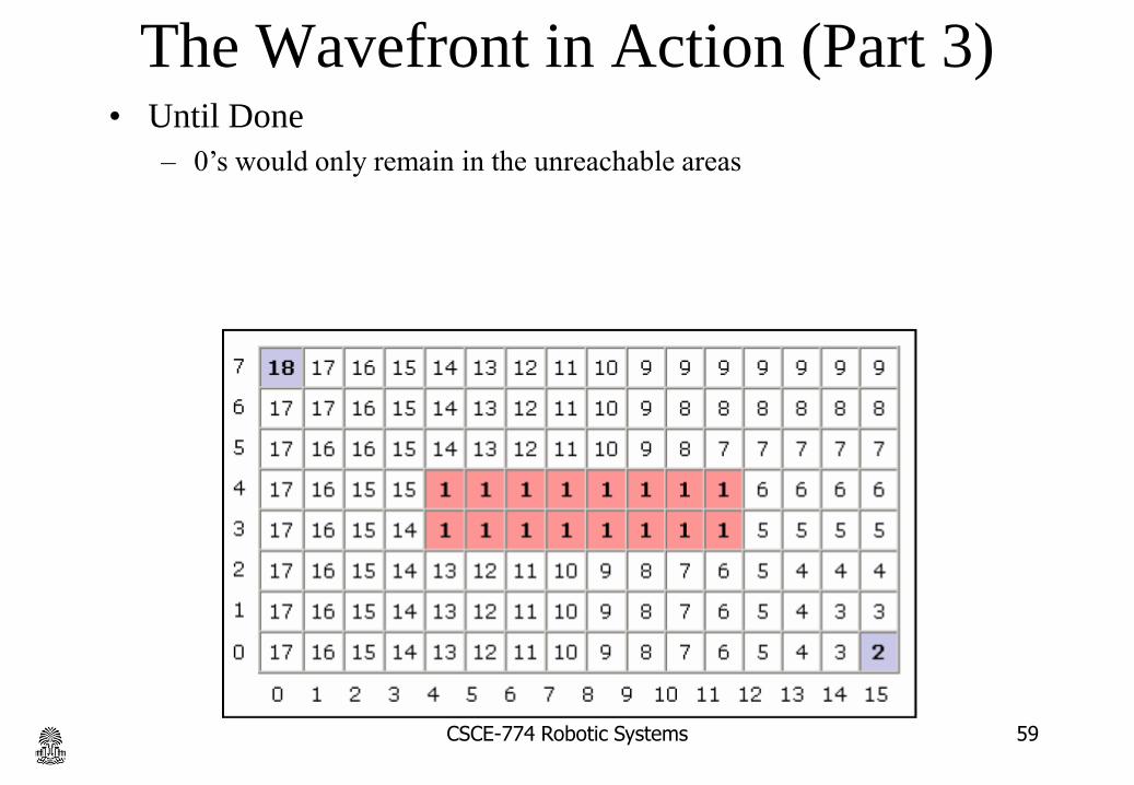
The Wavefront in Action (Part 3)• Until Done
– 0’s would only remain in the unreachable areas
CSCE-774 Robotic Systems 59
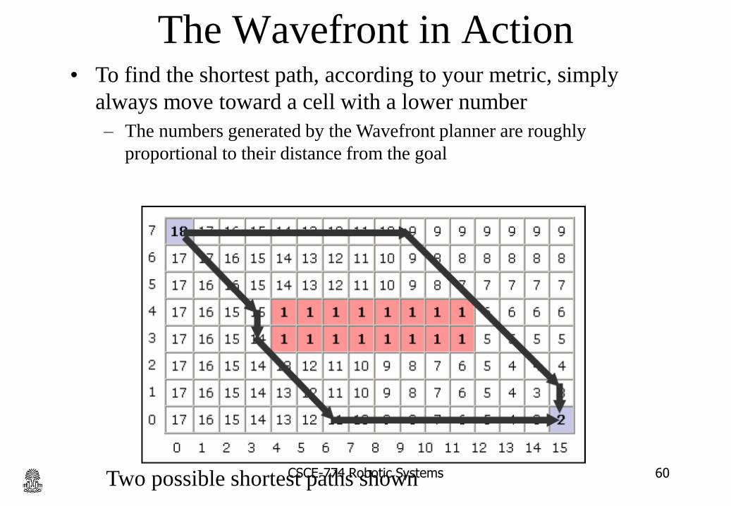
The Wavefront in Action• To find the shortest path, according to your metric, simply
always move toward a cell with a lower number
– The numbers generated by the Wavefront planner are roughly
proportional to their distance from the goal
Two possible shortest paths shownCSCE-774 Robotic Systems 60

An alternative roadmap
CSCE-774 Robotic Systems 61

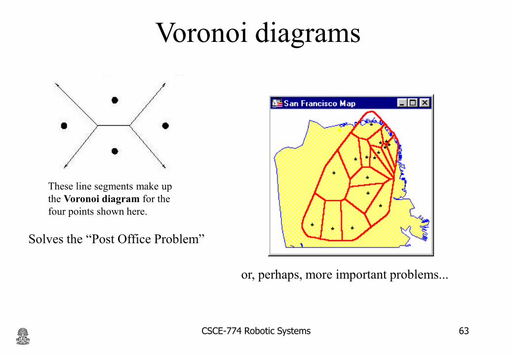
Voronoi diagrams
These line segments make up
the Voronoi diagram for the
four points shown here.
Solves the “Post Office Problem”
CSCE-774 Robotic Systems 62
Voronoi diagrams
These line segments make up
the Voronoi diagram for the
four points shown here.
Solves the “Post Office Problem”
or, perhaps, more important problems...
CSCE-774 Robotic Systems 63
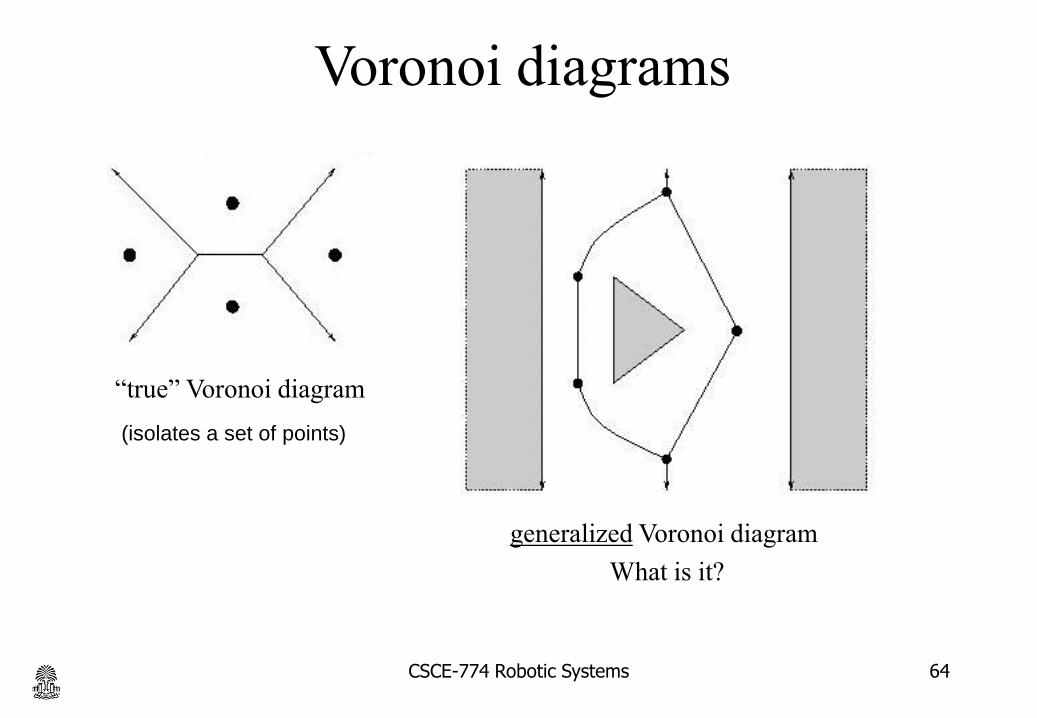
Voronoi diagrams
“true” Voronoi diagram
generalized Voronoi diagram
What is it?
(isolates a set of points)
CSCE-774 Robotic Systems 64
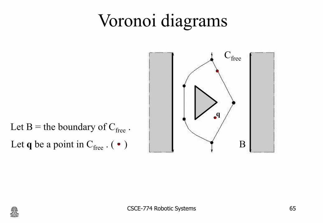
Voronoi diagrams
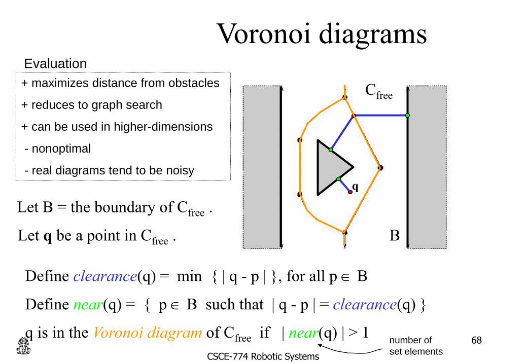
Let B = the boundary of Cfree .
Let q be a point in Cfree . ( )
Cfree
q
B
CSCE-774 Robotic Systems 65

Voronoi diagrams
Let B = the boundary of Cfree .
Let q be a point in Cfree .
Cfree
q
Define clearance(q) = min { | q - p | }, for all p B
B
CSCE-774 Robotic Systems 66

Voronoi diagrams
Let B = the boundary of Cfree .
Let q be a point in Cfree .
Cfree
q
Define clearance(q) = min { | q - p | }, for all p B
B
Define near(q) = { p B such that | q - p | = clearance(q) }
CSCE-774 Robotic Systems 67
Voronoi diagrams
Let B = the boundary of Cfree .
Let q be a point in Cfree .
Cfree
q
Define clearance(q) = min { | q - p | }, for all p B
B
Define near(q) = { p B such that | q - p | = clearance(q) }
q is in the Voronoi diagram of Cfree if | near(q) | > 1number of
set elements
+ maximizes distance from obstacles
+ reduces to graph search
+ can be used in higher-dimensions
- nonoptimal
- real diagrams tend to be noisy
Evaluation
CSCE-774 Robotic Systems
68

Generalized Voronoi Graph (GVG)
Free SpaceCSCE-774 Robotic Systems 69

Generalized Voronoi Graph (GVG)
Free Space with Topological Map (GVG)
CSCE-7
74 R
obotic
Syst
em
s
70
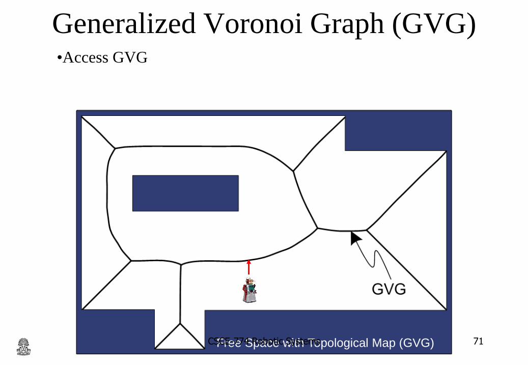
Generalized Voronoi Graph (GVG)
Free Space with Topological Map (GVG)
•Access GVG
71CSCE-774 Robotic Systems
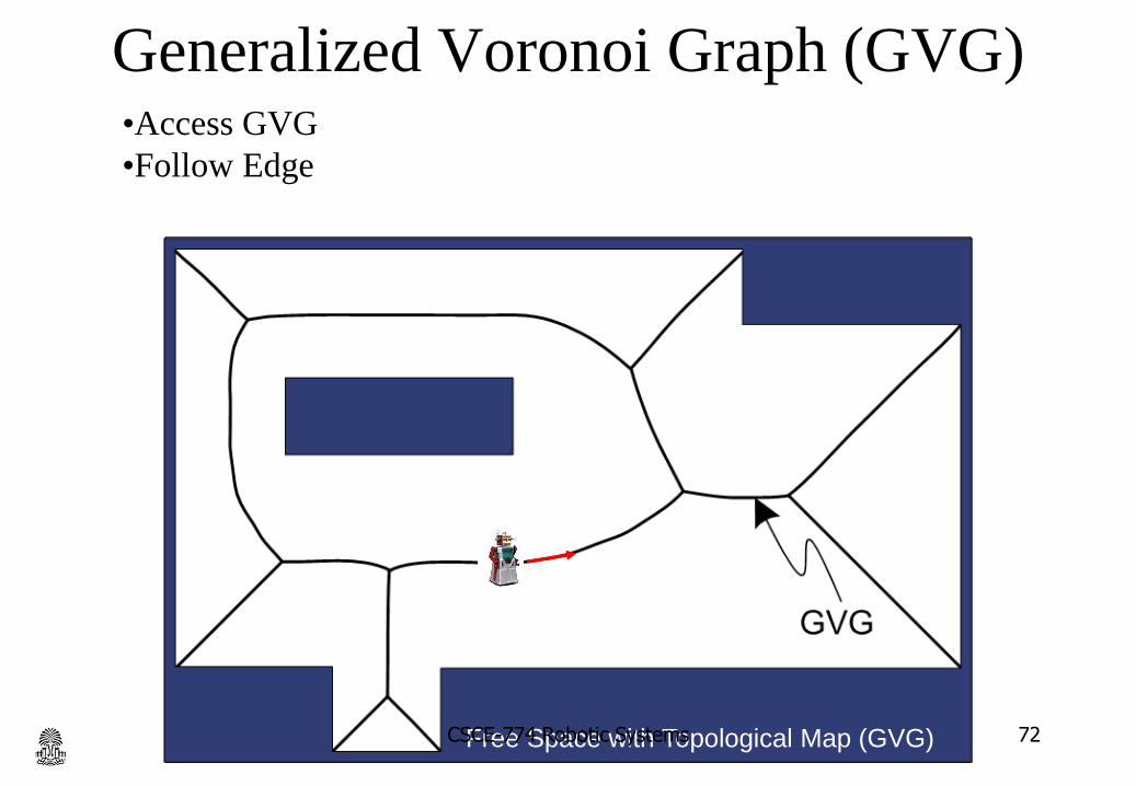
Generalized Voronoi Graph (GVG)
Free Space with Topological Map (GVG)
•Access GVG
•Follow Edge
CSCE-774 Robotic Systems 72
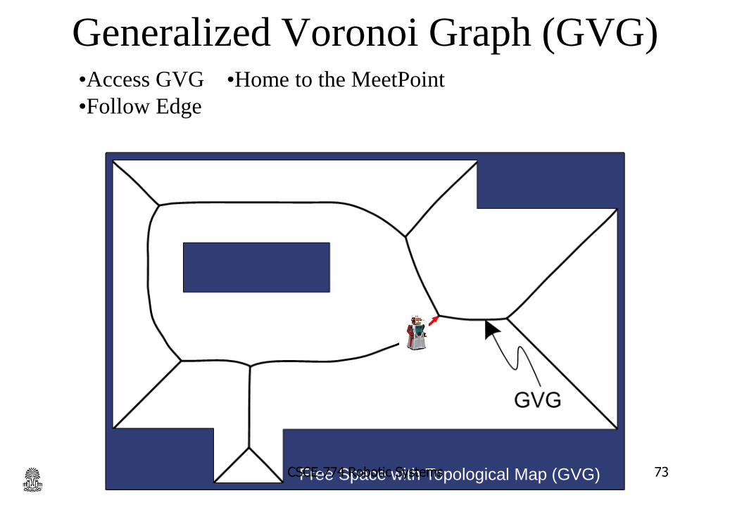
Generalized Voronoi Graph (GVG)
Free Space with Topological Map (GVG)
•Access GVG
•Follow Edge
•Home to the MeetPoint
CSCE-774 Robotic Systems 73

Generalized Voronoi Graph (GVG)
Free Space with Topological Map (GVG)
•Access GVG
•Follow Edge
•Home to the MeetPoint
•Select Edge
CSCE-774 Robotic Systems 74

• Nomadic Scout
• Sonar (GVG navigation)
• Camera with omni-directional
mirror (feature detection)
• Onboard 1.2 GHz processor
GVG construction using sonar
CSCE-774 Robotic Systems 75
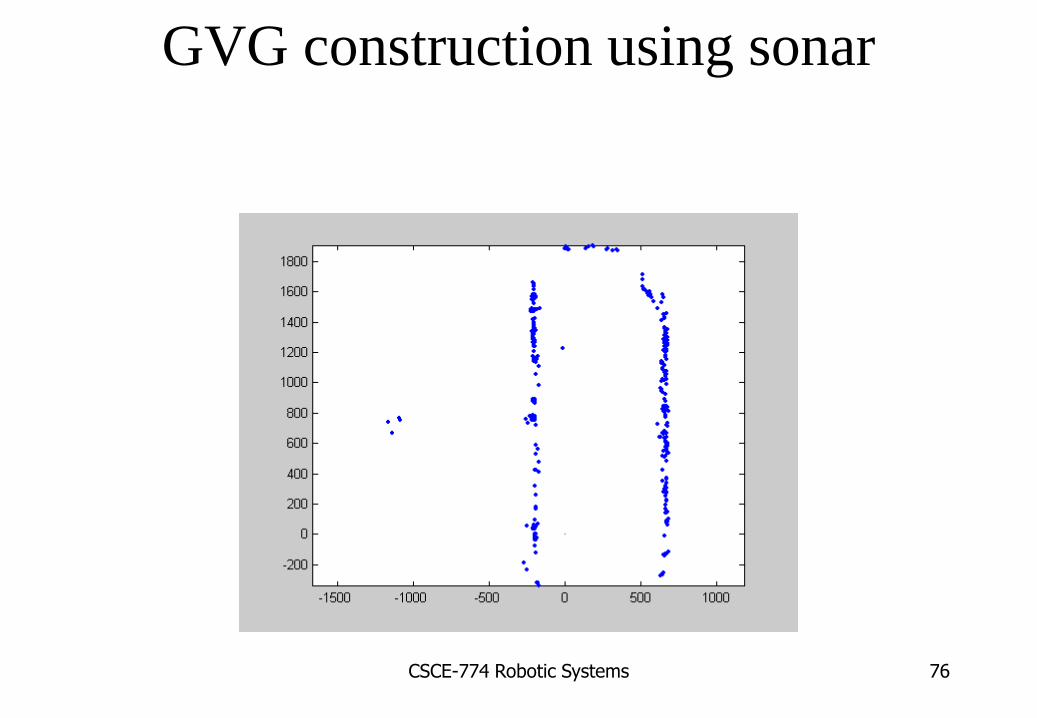
GVG construction using sonar
CSCE-774 Robotic Systems 76

GVG construction using sonar
CSCE-774 Robotic Systems 77

Slammer in Action
CSCE-774 Robotic Systems 78

Removing Edges
CSCE-774 Robotic Systems 79
Meetpoint Detection
• 3σ uncertainty ellipse of explored meetpoints
• Meetpoint degree (branching factor)
• Distances to local obstacles
• Relative angle bearings
• Edge signature
– Edge length
– Edge Curvature
• Vertex signal
CSCE-774 Robotic Systems 80
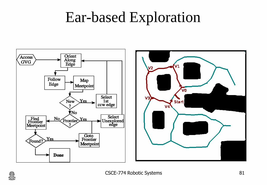
Ear-based Exploration
CSCE-774 Robotic Systems 81

Uncertainty Reduction
CSCE-774 Robotic Systems 82
Before Loop-closure After Loop-closure

Simulation
CSCE-774 Robotic Systems 83
Code available online at https://github.com/QiwenZhang/gvg
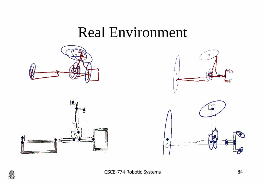
Real Environment
CSCE-774 Robotic Systems 84

Ear-based Exploration on
Hybrid Metric/Topological Maps
CSCE-774 Robotic Systems 85

Voronoi applications
Skeletonizations resulting from
constant-speed curve evolution
A retraction of a 3d object
== “medial surface” what?
in 2d, it’s called
a medial axisCSCE-774 Robotic Systems 86

skeleton shape
again reduces a 2d (or higher) problem to a question about graphs...
curve evolution centers of maximal diskswhere wavefronts collide
CSCE-774 Robotic Systems 87
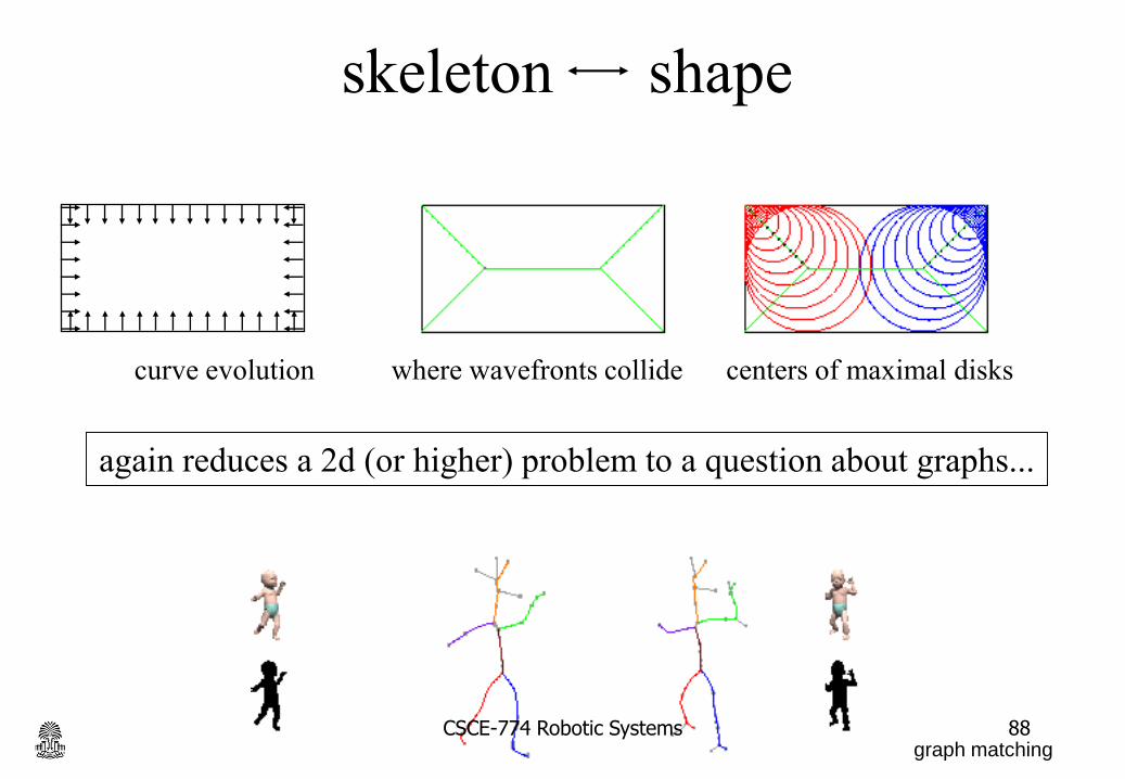
skeleton shape
again reduces a 2d (or higher) problem to a question about graphs...
curve evolution centers of maximal diskswhere wavefronts collide
graph matchingCSCE-774 Robotic Systems 88

Problems
The skeleton is sensitive to small changes in the object’s boundary.
- graph isomorphism (and lots of other graph questions) : NP-completeCSCE-774 Robotic Systems 89

Roadmap problems
If an obstacle decides to roll away... (or wasn’t there to begin with)
recomputing in less than O(N2) time?CSCE-774 Robotic Systems 90