cse 554 lecture 7: simplification
DESCRIPTION
CSE 554 Lecture 7: Simplification. Fall 2014. Geometry Processing. Fairing (smoothing) Relocating vertices to achieve a smoother appearance Method: centroid averaging Simplification Reducing vertex count Deformation Relocating vertices guided by user interaction or to fit onto a target. - PowerPoint PPT PresentationTRANSCRIPT

CSE554 Simplification Slide 1
CSE 554
Lecture 7: Simplification
CSE 554
Lecture 7: Simplification
Fall 2015
CSE554 Simplification Slide 2
Geometry ProcessingGeometry Processing
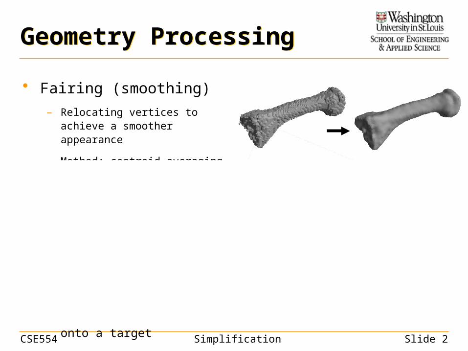
• Fairing (smoothing)
– Relocating vertices to achieve a smoother appearance
– Method: centroid averaging
• Simplification
– Reducing vertex count
• Deformation
– Relocating vertices guided by user interaction or to fit onto a target
CSE554 Simplification Slide 3
Simplification (2D)Simplification (2D)
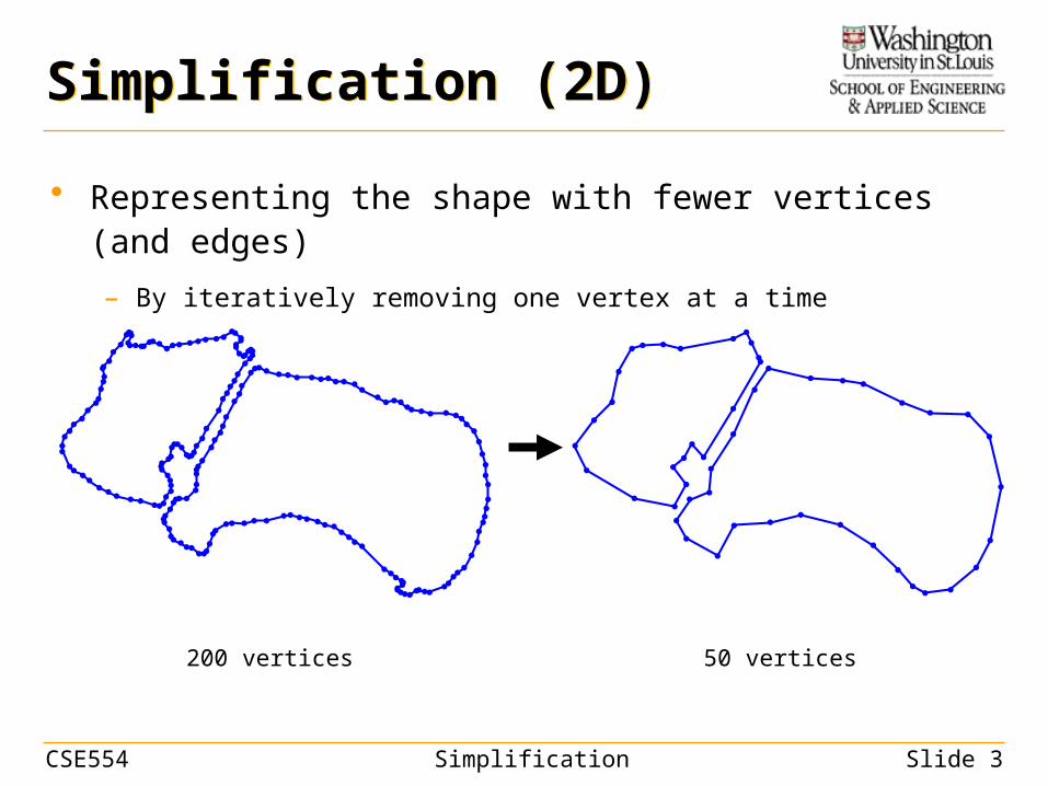
• Representing the shape with fewer vertices (and edges)
– By iteratively removing one vertex at a time
200 vertices 50 vertices
CSE554 Simplification Slide 4
Simplification (2D)Simplification (2D)
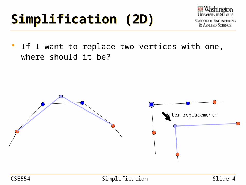
• If I want to replace two vertices with one, where should it be?
After replacement:

CSE554 Simplification Slide 5
Simplification (2D)Simplification (2D)
• If I want to replace two vertices with one, where should it be?
– Shortest distances to the supporting lines of involved edges
After replacement:

CSE554 Simplification Slide 6
• Same representation
• Different meaning:
– Point: a fixed location (relative to {0,0} or {0,0,0})
– Vector: a direction and magnitude
• No location (any location is possible)
Points and VectorsPoints and Vectors
x, y or x, y, zx
Y
1
2
2
p 1, 2 p 2, 2
v
1, 2v
1, 2
CSE554 Simplification Slide 7
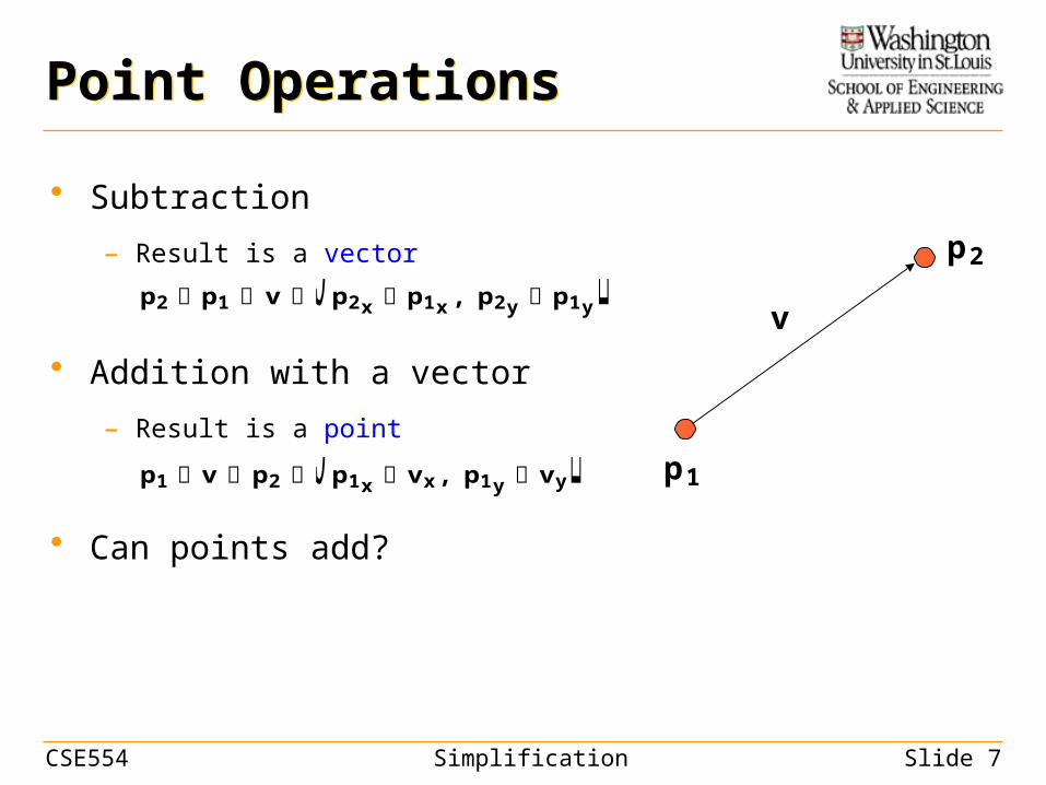
• Subtraction
– Result is a vector
• Addition with a vector
– Result is a point
• Can points add?
Point OperationsPoint Operations
p1
p2
vp2 p1 v p2x p1x, p2y p1yp1 v p2 p1x vx, p1y vy

CSE554 Simplification Slide 8
Adding PointsAdding Points
• Affine combinations
– Weighted addition of points where all weights sum to 1
– Result is another point
• Same as adding scaled vectors to a point
ni1
wi pi p, where ni1
wi 1 p1
p2
p3p4
p
ni1
wi pi ni1
wi pi p1 ni1
wi p1
ni1
wi vi p1
v2
v3 v4

CSE554 Simplification Slide 9
Adding PointsAdding Points
• Affine combinations: examples
– Mid-point of two points
– Linear interpolation of two points
– Centroid of multiple points
p p1 p2
2
p 1 p1 p2
p ni1
pi
n
p
p1
p2
pp1
p2
1
p1p2
p3 p4
p

CSE554 Simplification Slide 10
• Addition/Subtraction
– Result is a vector
• Scaling by a scalar
– Result is a vector
• Magnitude
– Result is a scalar
• A unit vector:
• To make a unit vector (normalization):
Vector OperationsVector Operations
v1
v2
v 1v 2 v1
v2
v1 v
2
vsv
v1 v2 v1x v2x, v1y v2ys v s vx, s vyv vx
2 vy2
v 1v
v

CSE554 Simplification Slide 11
• Dot product (in both 2D and 3D)
– Result is a scalar
– In coordinates (simple!)
• 2D:
• 3D:
• Matrix product between a row and a column vector
More Vector OperationsMore Vector Operations
v1
v2
v1 v2 v1x v2x v1y v2y v1z v2z
v1 v2 v1 v2 Cosv1 v2 v1x v2x v1y v2y
CSE554 Simplification Slide 12
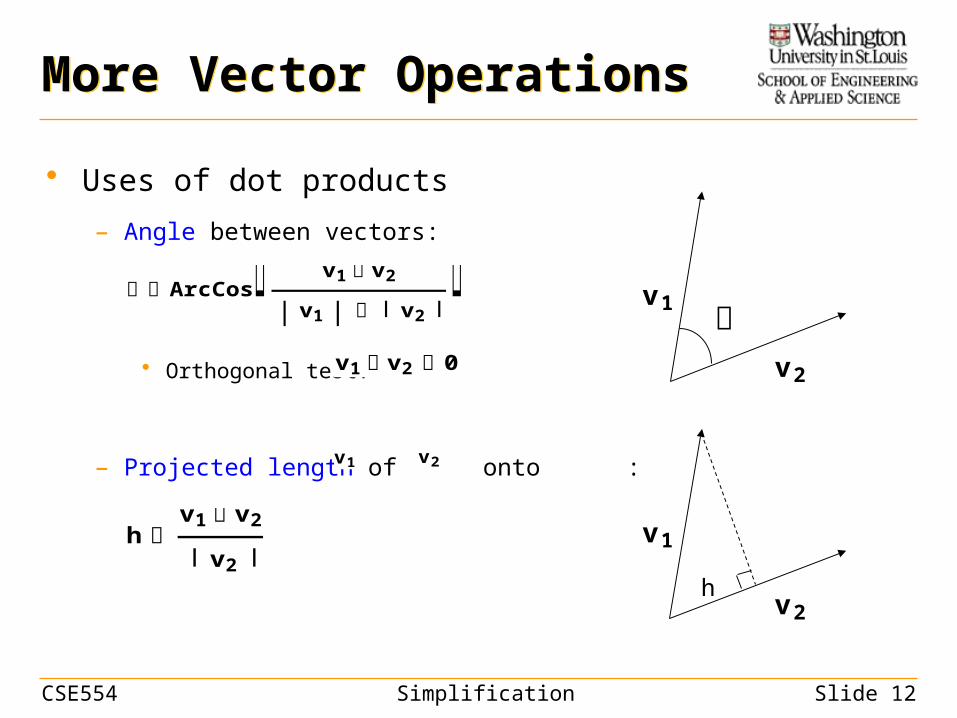
• Uses of dot products
– Angle between vectors:
• Orthogonal test:
– Projected length of onto :
More Vector OperationsMore Vector Operations
v1
v2
v1
v2h
v1 v2
ArcCos v1 v2
v1 v2
v1 v2 0
h v1 v2
v2

CSE554 Simplification Slide 13
• Cross product (only in 3D)
– Result is another 3D vector
• Direction: Normal to the plane where both vectors lie (right-hand rule)
• Magnitude:
– In coordinates:
More Vector OperationsMore Vector Operations
v1
v2
v1 v2 v1 v2 Sinv1 v2
v1y v2z v1z v2y, v1z v2x v1x v2z, v1x v2y v1y v2x v1v2

CSE554 Simplification Slide 14
More Vector OperationsMore Vector Operations
• Uses of cross products
– Getting the normal vector of the plane
• E.g., the normal of a triangle formed by
– Computing area of the triangle formed by
• Testing if vectors are parallel:
v1v2
v1v2
v1
v2Area v1 v2
2
v1 v2 0
v1v2

CSE554 Simplification Slide 15
PropertiesProperties
Dot Product Cross Product
Distributive?
Commutative?
Associative?
(Sign change!)
v v1 v2 v v1 v v2
v v1 v2 v v1 v v2
v1 v2 v2 v1 v1 v2 v2 v1
v1 v2 v3 v1 v2 v3v1 v2 v3

CSE554 Simplification Slide 16
Simplification (2D)Simplification (2D)
• Distance to a line
– Line represented as a point q on the line, and a perpendicular unit vector (the normal) n
• To get n: take a vector {x,y} along the line, n is {-y,x} followed by normalization
– Distance from any point p to the line:
• Projection of vector (p-q) onto n
– This distance has a sign
• “Above” or “under” of the line
• We will use the distance squared
p q n
p
q
n
CSE554 Simplification Slide 17
Simplification (2D)Simplification (2D)
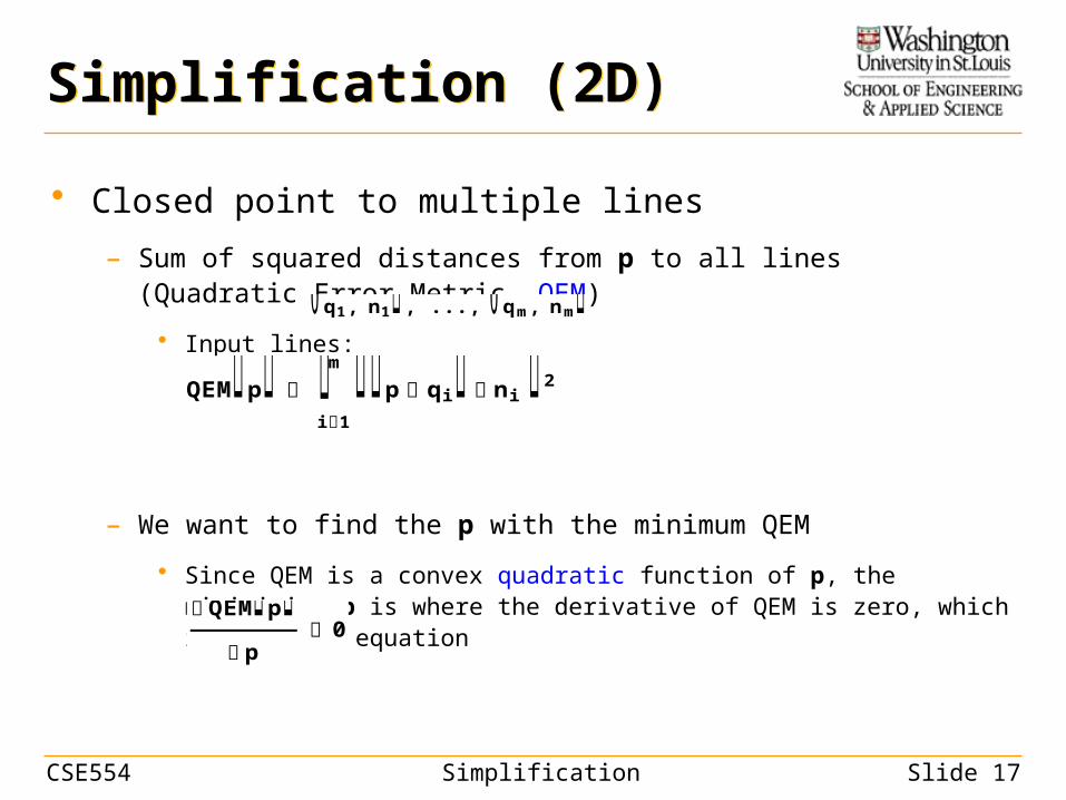
• Closed point to multiple lines
– Sum of squared distances from p to all lines (Quadratic Error Metric, QEM)
• Input lines:
– We want to find the p with the minimum QEM
• Since QEM is a convex quadratic function of p, the minimizing p is where the derivative of QEM is zero, which is a linear equation
QEMp i1
m p qi ni 2 q1, n1, ..., qm, nm
QEMp p
0

CSE554 Simplification Slide 18
Simplification (2D)Simplification (2D)
• Minimizing QEM
– Writing QEM in matrix form
2x2 matrix 1x2 column vector Scalar
a
mi1
nix nix mi1
nix niy mi1
nix niy mi1
niy niyb
mi1
nix ni qi mi1
niy ni qi c mi1
ni qi2
p px py QEMp p a pT 2 p b c [Eq. 1]
Matrix (dot) product
Row vectorMatrix transpose
QEMp i1
m p qi ni 2

CSE554 Simplification Slide 19
Simplification (2D)Simplification (2D)
• Minimizing QEM
– Solving the zero-derivative equation:
– A linear system with 2 equations and 2 unknowns (px,py)
• Using Gaussian elimination, or matrix inversion:
QEMp p
2 a pT 2 b 0
a pT b m
i1nix nix m
i1nix niy m
i1nix niy m
i1niy niy
pxpy
m
i1nix ni qi m
i1niy ni qi
[Eq. 2]
pT a1 b
QEMp p a pT 2 p b c
CSE554 Simplification Slide 20
Simplification (2D)Simplification (2D)
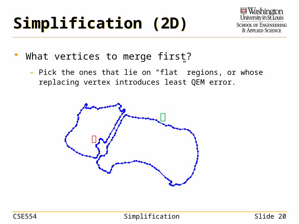
• What vertices to merge first?
– Pick the ones that lie on “flat” regions, or whose replacing vertex introduces least QEM error.
CSE554 Simplification Slide 21
Simplification (2D)Simplification (2D)
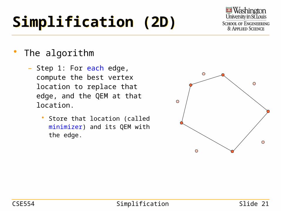
• The algorithm
– Step 1: For each edge, compute the best vertex location to replace that edge, and the QEM at that location.
• Store that location (called minimizer) and its QEM with the edge.

CSE554 Simplification Slide 22
Simplification (2D)Simplification (2D)
• The algorithm
– Step 1: For each edge, compute the best vertex location to replace that edge, and the QEM at that location.
• Store that location (called minimizer) and its QEM with the edge.
– Step 2: Pick the edge with the lowest QEM and collapse it to its minimizer.
• Update the minimizers and QEMs of the re-connected edges.

CSE554 Simplification Slide 23
Simplification (2D)Simplification (2D)
• The algorithm
– Step 1: For each edge, compute the best vertex location to replace that edge, and the QEM at that location.
• Store that location (called minimizer) and its QEM with the edge.
– Step 2: Pick the edge with the lowest QEM and collapse it to its minimizer.
• Update the minimizers and QEMs of the re-connected edges.

CSE554 Simplification Slide 24
Simplification (2D)Simplification (2D)
• The algorithm
– Step 1: For each edge, compute the best vertex location to replace that edge, and the QEM at that location.
• Store that location (called minimizer) and its QEM with the edge.
– Step 2: Pick the edge with the lowest QEM and collapse it to its minimizer.
• Update the minimizers and QEMs of the re-connected edges.
– Step 3: Repeat step 2, until a desired number of vertices is left.

CSE554 Simplification Slide 25
Simplification (2D)Simplification (2D)
• The algorithm
– Step 1: For each edge, compute the best vertex location to replace that edge, and the QEM at that location.
• Store that location (called minimizer) and its QEM with the edge.
– Step 2: Pick the edge with the lowest QEM and collapse it to its minimizer.
• Update the minimizers and QEMs of the re-connected edges.
– Step 3: Repeat step 2, until a desired number of vertices is left.

CSE554 Simplification Slide 26
Simplification (2D)Simplification (2D)
• Step 1: Computing minimizer and QEM on an edge
– Consider supporting lines of this edge and adjacent edges
– Compute and store at the edge:
• The minimizing location p (Eq. 2)
• QEM (substitute p into Eq. 1)
– Used for edge selection in Step 2
• QEM coefficients (a, b, c)
– Used for fast update in Step 2Stored at the edge:
p
a, b, c, p, QEMpQEMp p a pT 2 p b c [Eq. 1]

CSE554 Simplification Slide 27
Simplification (2D)Simplification (2D)
• Step 2: Collapsing an edge
– Remove the edge and its vertices
– Re-connect two neighbor edges to the minimizer of the removed edge
– For each re-connected edge:
• Increment its coefficients by that of the removed edge
– The coefficients are additive!
• Re-compute its minimizer and QEM
a, b, c,
p, QEMp a1, b1, c1,
p1, QEMp1 a2, b2, c2,
p2, QEMp2
p
a a1,b b1,c c1,p1, QEMp1
a a2,b b2,c c2,p2, QEMp2
Collapse
: new minimizer locations computed from the updated coefficients
p1, p2
a a1,b b1,c c1,p1, QEMp1
a a2,b b2,c c2,p2, QEMp2
CSE554 Simplification Slide 28
Simplification (3D)Simplification (3D)
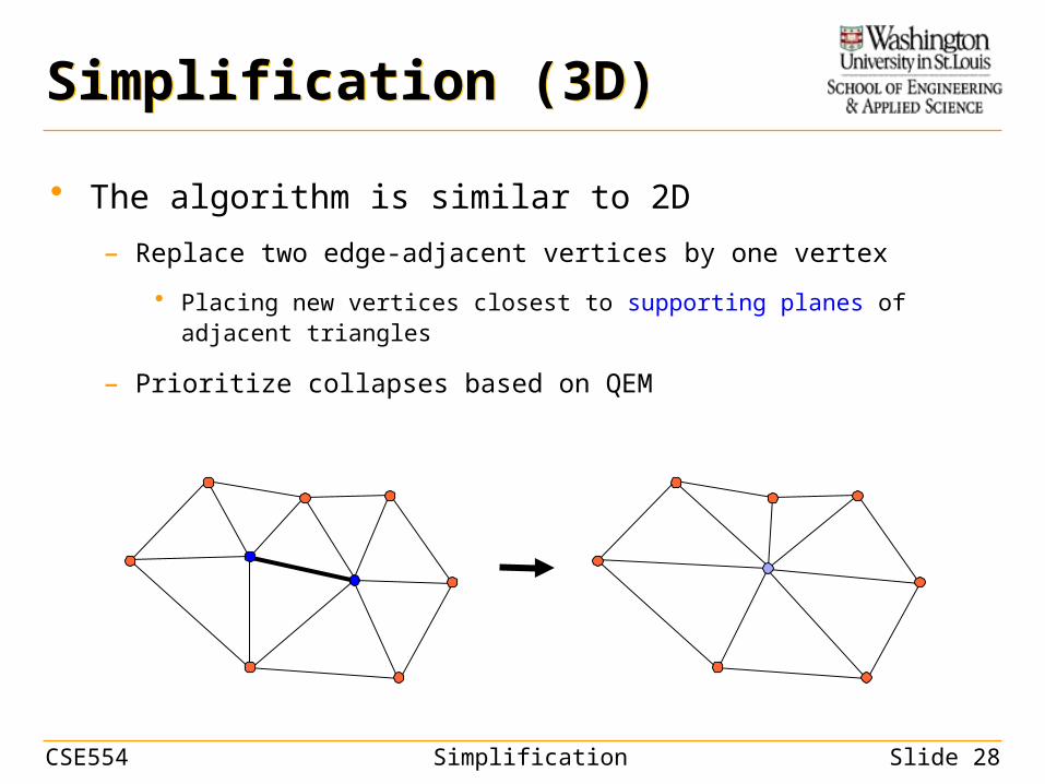
• The algorithm is similar to 2D
– Replace two edge-adjacent vertices by one vertex
• Placing new vertices closest to supporting planes of adjacent triangles
– Prioritize collapses based on QEM
CSE554 Simplification Slide 29
Simplification (3D)Simplification (3D)
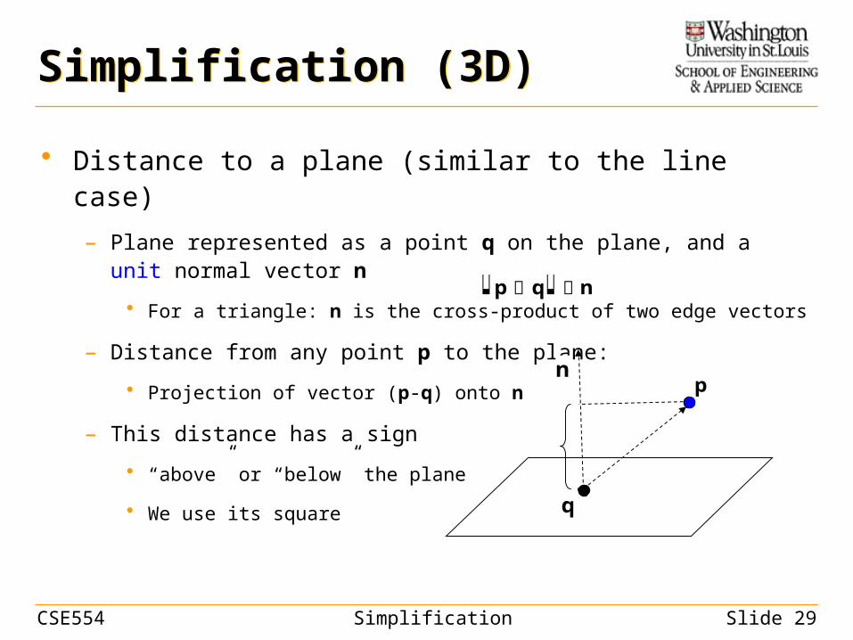
• Distance to a plane (similar to the line case)
– Plane represented as a point q on the plane, and a unit normal vector n
• For a triangle: n is the cross-product of two edge vectors
– Distance from any point p to the plane:
• Projection of vector (p-q) onto n
– This distance has a sign
• “above” or “below” the plane
• We use its square
p q n
p
q
n

CSE554 Simplification Slide 30
Simplification (3D)Simplification (3D)
• Closest point to multiple planes
– Input planes:
– QEM (same as in 2D)
• In matrix form:
– Find p that minimizes QEM:
• A linear system with 3 equations and 3 unknowns (px,py,pz)
QEMp p a pT 2 p b c
p px py pz q1, n1, ..., qm, nm
3x3 matrix
1x3 column vector
Scalar
a
m
i1nix nix m
i1nix niy m
i1nix niz m
i1niy nix m
i1niy niy m
i1niy niz m
i1niz nix m
i1niz niy m
i1niz niz
b
m
i1nix ni qi m
i1niy ni qi m
i1niz ni qi
c mi1
ni qi2a pT b
QEMp i1
m p qi ni 2

CSE554 Simplification Slide 31
Simplification (3D)Simplification (3D)
• Step 1: Computing minimizer and QEM on an edge
– Consider supporting planes of all triangles adjacent to the edge
– Compute and store at the edge:
• The minimizing location p
• QEM[p]
• QEM coefficients (a, b, c)
The supporting planes for all shaded triangles should be considered when computing the minimizer of the middle edge.
p
CSE554 Simplification Slide 32
Simplification (3D)Simplification (3D)
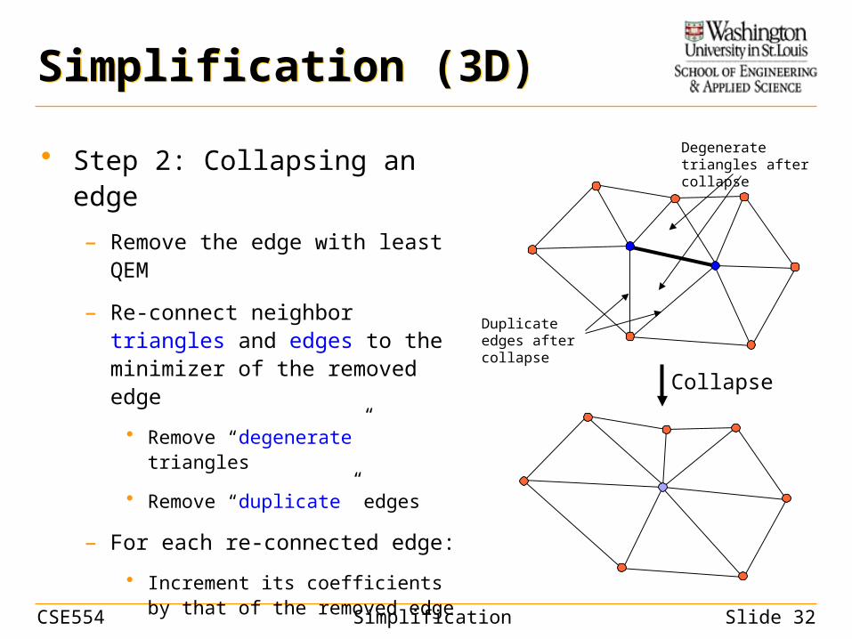
• Step 2: Collapsing an edge
– Remove the edge with least QEM
– Re-connect neighbor triangles and edges to the minimizer of the removed edge
• Remove “degenerate” triangles
• Remove “duplicate” edges
– For each re-connected edge:
• Increment its coefficients by that of the removed edge
• Re-compute its minimizer and QEM
Collapse
Degenerate triangles after collapse
Duplicate edges after collapse
CSE554 Simplification Slide 33
Simplification (3D)Simplification (3D)
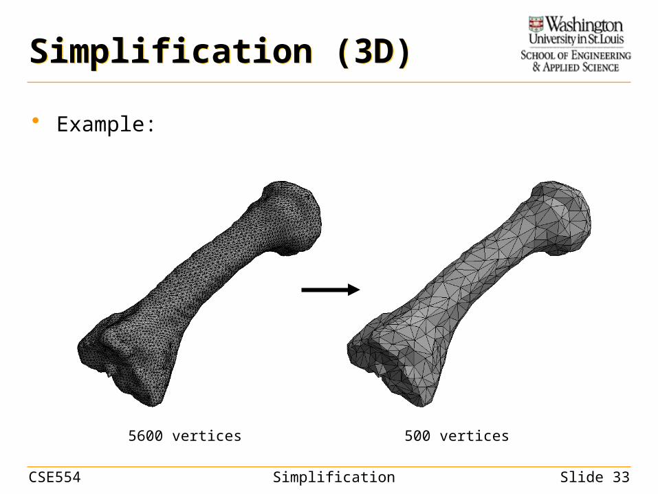
• Example:
5600 vertices 500 vertices
CSE554 Simplification Slide 34
Further ReadingsFurther Readings
• Fairing:
– “A signal processing approach to fair surface design”, by G. Taubin (1995)
• No-shrinking centroid-averaging
• Google citations > 1000
• Simplification:
– “Surface simplification using quadric error metrics”, by M. Garland and P. Heckbert (1997)
• Edge-collapse simplification
• Google citations > 2000