csce 990: real-time systems proportional share...

1

Rea

l-T

ime

Sys

tem

s P

rop

Shar

e -

1Je

ffay

/God

dardC

SC

E 9

90: R

eal-

Tim

e Sy

stem

s

Pro

port

iona

l Sha

reSc

hedu

ling

Stev

e G

odda

rdgo

ddar

d@cs

e.un

l.edu

htt

p:/

/ww

w.c

se.u

nl.e

du/~

god

dard

/Cou

rses

/Rea

lTim

eSys

tem

s

2

Real-Time Systems Prop Share - 2Jeffay/Goddard

Introduction

◆ We have looked at systems consisting exclusively ofhard real-time tasks and systems consisting of real-timeand non-real-time tasks.» In both cases, we assumed that all jobs were scheduled

according to normal real-time scheduling disciplines.

◆ We now look at another way of integrating real-timeand non-real-time computing: Fairness» Proportional Share Resource Allocation, Stoica et. al. (1996)

» P-fair Scheduling, Baruah et. al. (1996)

◆ We will show that the notion of Fairness can be used toexecute jobs in real-time.

3


◆ Processes are allocated a share of a shared resource:» a relative percentage of the resource’s total capacity.

◆ Processes make progress at a uniform rate according totheir share.

◆ OS Example — time sharing tasks allocated an equalshare (1/nth) of the processor’s capacity» round robin scheduling, fixed size quantum

0

T1

T2

q 2q 3q 4q 5q 6q 7q 8q 9q 10q 11q 12q 13q

T3

Proportional Share Concept

4


◆ Processes are allocated a share of the processor’scapacity:» Process i is assigned a weight wi

• Note: wi is a rational number. That is, it need not be aninteger.

» Process i’s share of the CPU at time t is

fi(t) =

• Note: in the denominator of fi(t) we are summing overonly the active processes in the system; all tasks in thecase of a real-time system.

Σj wj

wi

Formal Allocation Model

5


◆ If processes’ weights remain constant in [t1, t2] thenprocess i receives

units of execution time in [t1, t2] for a fluid-allocationsystem.

◆ Some comments on Si(t1,t2):» The definition of the integral Si() is always correct.» The assumption that weights remain constant over the

interval lets us reduce the integral to a linear equation.» Otherwise, we can generate a piecewise linear equation.

Formal Allocation Model

Si(t1,t2) = = (t2 - t1)Σj wj

wi∫2

1

)(t

t

i dtf τ

6


Real-Time Scheduling Example

◆ Ignoring weights for a moment, we note that Al Mok gave asimple proof (in his dissertation) that utilization ≤ 1 is asufficient condition for schedulability when each task Ti isallocated a fraction of each time unit equal to its utilization ei/pi.

◆ Thus, we can schedule periodic tasks with a round robinscheduling algorithm if we assume an infinitesimally smallquantum and allocate each task a share equal to their processorutilization ei/pi within each time unit.

0

T1 = (8, 2)

T2 = (6, 3)

1 2 3 4 5 6 7 8 9 10 11 12 13

0.5

0.25

7


◆ Now consider the same task set with RR schedulingand a variable-sized quantum. Assume a round lengthof 2.

◆ Thus, the share of task Ti in each round (of length 2) is2(ei/pi).

◆ Note: This slide and the rest of the presentation on ProportionalShare uses a slightly different notation for the release anddeadline of a task:» down arrows represent releases (or a job entering the system).» up arrows represent deadlines (or a job leaving the system).

0 1 2 3 4 5 6 7 8 9 10 11 12 13

T1 = (8, 2)

T2 = (6, 3)

0.5

1.0


8


◆ Round robin scheduling with an integer, variable-sizedquantum and a round length of 4:

◆ Notice that, in this and the last two examples, theprocessor is idle at least 25% of each round, even whenthere are ready tasks.» In these examples, the scheduling algorithm is non-work-

conserving.◆ However, each process always receives its share in each

round.

0

T1 = (8, 2)

T2 = (6, 3)

1 2 3 4 5 6 7 8 9 10 11 12 13

1.0

2.0 1.0


9


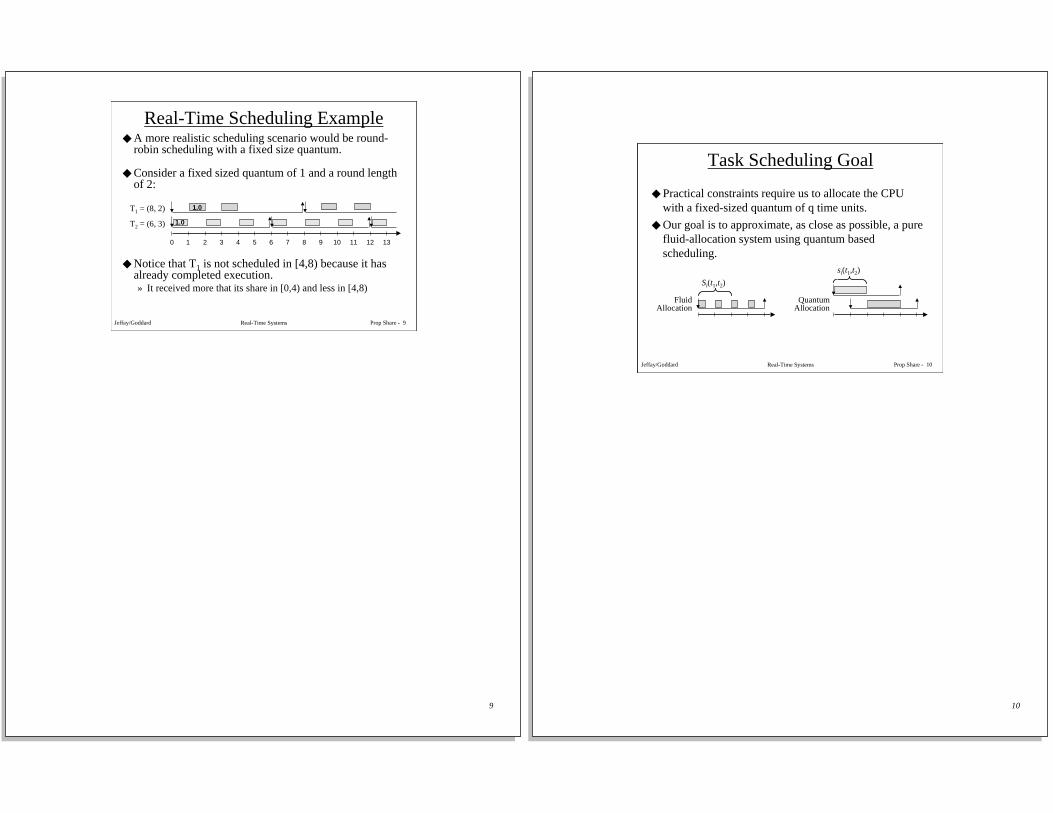
◆ A more realistic scheduling scenario would be round-robin scheduling with a fixed size quantum.

◆ Consider a fixed sized quantum of 1 and a round lengthof 2:

◆ Notice that T1 is not scheduled in [4,8) because it hasalready completed execution.» It received more that its share in [0,4) and less in [4,8)

0

T1 = (8, 2)

T2 = (6, 3)

1 2 3 4 5 6 7 8 9 10 11 12 13

1.0

1.0


10


Task Scheduling Goal

◆ Practical constraints require us to allocate the CPUwith a fixed-sized quantum of q time units.

◆ Our goal is to approximate, as close as possible, a purefluid-allocation system using quantum basedscheduling.

QuantumAllocation

FluidAllocation

Si(t1,t2)

si(t1,t2)

11


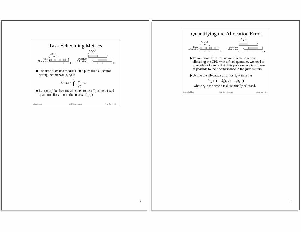
Task Scheduling Metrics

◆ The time allocated to task Ti in a pure fluid allocationduring the interval [t1,t2) is

◆ Let si(t1,t2) be the time allocated to task Ti using a fixedquantum allocation in the interval [t1,t2).

Si(t1,t2) = dτ Σjwj

wi∫2

1

t

t

QuantumAllocation

FluidAllocation

Si(t1,t2)

si(t1,t2)

12


◆ To minimize the error incurred because we areallocating the CPU with a fixed quantum, we need toschedule tasks such that their performance is as closeas possible to their performance in the fluid system.

◆ Define the allocation error for Ti at time t as

lagi(t) = Si(t0,t) – si(t0,t)where t0 is the time a task is initially released.

Quantifying the Allocation Error

QuantumAllocation

FluidAllocation

Si(t1,t2)

si(t1,t2)

13


◆ Because allocation is quantum-based, tasks can be eitherbehind or ahead of the fluid schedule.» If lag is negative then a task has received more service time

than it would have received in the fluid system.

» If lag is positive then a task has received less service time thanit would have received in the fluid system.

lagi(t) = Si(t0,t) – si(t0,t)

QuantumAllocation

FluidAllocation

Si(t1,t2)

si(t1,t2)

What Does lagi(t) Mean?

14


◆ Goal: Schedule tasks such that theirperformance is as close as possible to that inthe fluid system

◆ Schedule tasks such that the lag is:» bounded, and» minimized over all tasks and time intervals

lagi(t) = Si(t0,t) – si(t0,t)

QuantumAllocation

FluidAllocation

Si(t1,t2)

si(t1,t2)

Real-Time Computing using Proportional Share

15


Issues

◆ What happens when a task’s period/deadline is smallrelative to the size of a quantum?

◆ A large quantum is more efficient, but it introduces alarger allocation error.

◆ For example, a task’s lag can be negative when» The quantum is large and the task executes very soon after

being released.

» Some other task does not use the share of the CPU that it isallocated (i.e., the task finishes “early”) and the task inquestion consumes the left-over capacity.

◆ Under what conditions is a task’s lag positive?

16


◆ Tasks are scheduled in a virtual time domain

◆ Each task executes for wi real-time units during each virtualtime unit.

VirtualTimeV(t)

t

t

Real-Time

t t

Σjwj

1 = 1

Σjwj t

Σjwj t

Σjwj

1 > 1Σjwj

1 < 1

t t

Scheduling to Bound Lag

V(t) = dτΣjwj

1∫t

0

17


◆ Slope of virtual timechanges as (non-real-time) tasks enter andleave the system

VirtualTimeV(t)

Real-Time

Σjwj

1 < 1

w1

w2

w3

The Virtual Time Domain

V(t) = dτΣjwj

1∫t

0

18


◆ Tasks execute for wi real-time time units in eachvirtual-time time unit» Thus ideally, task Ti

executes for

time units in any real-timeinterval

V(t)

Real-Time

1

Σjwj

Σjwj

1 < 1

w1

w2

w3

The Virtual Time Domain

Si(t1,t2) = wi dτ

= (V(t2) – V(t1))wi

Σjwj

1∫2

1

t

t

19


◆ Schedule tasks only when their lag is non-negative» If a task with negative lag makes a request for execution at

time t, it is not considered until a future time t’ when lag(t’) ≥ 0

» Let e > t be the earliest time a task can be scheduled

• the time at which S(ti, e) = s(ti, t)» This time occurs in the virtual time domain at time S(ti, e) = s(ti, t) (V(e) – V(ti))wi = s(ti, t) V(e) = V(ti) + s(ti,t)/wi

dτ

lagi = Si(t1,t2) – si(t1,t2)

Σj wj

wiSi(t1,t2) = ∫2

1

t

t

Virtual time scheduling principlesq

20


◆ Task requests should not be considered beforetheir “eligible” time e. Why?

◆ Requests should be completed by virtual timeV(d) = V(e) + ci/wi

» where ci is the cost of executing the request.

◆ Our candidate scheduling algorithm: EarliestEligible Virtual Deadline First (EEVDF)

At each scheduling point, a new quantumis allocated to the eligible task with the

earliest virtual deadline

Virtual time scheduling principles

21


Cost = 2

0real-time

1 2 3 4 5 6 7

(V(e),V(d)) = (0,1)

(.5,1)

virtual timeat time 0

0 0.5 1

Cost = 1

Example: Two tasks with equal weight = 2 (q = 1 in real-time). These tasks arenot periodic, but each task makes a request immediately after it completes. Thefirst task arrives at (real) time 0 and the second at (real) time 1.

EEVDF Scheduling

V(d) = V(e) + c/w

V(e) = V(t0) + s(t0 , t)/w dτΣj wj

1V(t) = ∫

t

0

There are two unit of real timeper unit of virtual time until V(0.5).

22

Note: These are not periodic tasks! (The arrows just indicate when tasks enter and leave the system.

In particular, assume that a task makes its next request immediately after it completes.

Note that:

— task 1 always has a virtual deadline 1 time unit after its eligible time (it requires one virtual timeunit to complete)

— task 2 always has a virtual deadline 0.5 time units after its eligible time


Cost = 2

0real-time

1 2 3 4 5 6 7

(V(e),V(d)) = (0,1) (1,2) (2,3)

(.5,1) (1,1.5) (1.5,2) (2,2.5)

virtual timeat time 0

0 0.5 1

Cost = 1

at time 0.50 0.5 1 1.5 2

At time V(0.5) = 1, virtual time slows down to four units of real time per unitof virtual time because we continually have two jobs, each with weight 2.

EEVDF Scheduling

V(d) = V(e) + c/w

V(e) = V(t0) + s(t0 , t)/w dτΣj wj

1V(t) = ∫

t

0

Jobs from task 2 arrive as soon as theprevious jobs are finished, but they are noteligible until 0.25 virtual time units later.

23


◆ To use proportional share scheduling for real-time computing:» We need to ensure deadlines are respected in the

real-time domain.

» We must also bound the allocation error.

Issues

24


Using Proportional Share AllocationFor Real-Time Computing

◆ Deadlines in a proportional share system ensureuniformity of allocation, not timeliness

◆ Weights are used to allocate a relative fraction of theCPU’s capacity to a task

fi(t) =

◆ Real-time tasks require a constant fraction of aresource’s capacity

fi(t) =◆ Thus real-time performance can be achieved by

adjusting weights dynamically so that the share remainsconstant

Σj wj

wi

pi

ci

25


Dynamically Adjusting Weights toSupport Real-Time Computing

◆ Consider task Ti that arrives at time t with adeadline at time t + di

» In the interval [t, t+di] the task requires a share ofthe processor equal to ci/di

t t + d

V(d) = V(e) + c/wi

V(e) = V(t) + s(t , t)/wi = V(t)

c

Σjwj

wi

di

ci=

wi = (Σj≠ iwj + wi)di

ci

di

ci Σj≠ iwj

di

ci1 – wi =

26


Dynamically Adjusting Weights toSupport Real-Time Computing

◆ Example: task Ti = (t,4,1,4) joins a system with a totalweight of 3 at time t with a deadline at time t + 4.» In the interval [t, t+4] the task requires a share of the

processor equal to 1/4=0.25.

» Its weight should be

di

ci Σj≠ iwj

di

ci1 – wi = 4

1 x 3

41

1 – = = 1

27


Issues

◆ Every time the slope of the virtual time changes, wemust recompute the weight and deadline for the task.

» Will its lag change?

◆ If there are a n real-time tasks then we end up with nlinear equations with n unknowns.

◆ If real-time tasks require a fixed share of the CPU’scapacity, only a finite number of tasks may beguaranteed to execute in real-time.

» How do we limit the number of real-time tasks?

28


◆ We need simple (efficient) on-line admissioncontrol algorithm!

◆ Admission criterion:» a simple sufficient condition —

» a necessary condition??• it depends...

Σi ≤ 1di

ci

Admission control

29


◆ Is a task guaranteed to complete before itsdeadline?

◆ How late can a task be?

q

Bounding the Allocation Error

Theorem: A task will miss its deadline by at most qtime units.

30


◆ Consider a task system wherein jobs always terminatewith zero lag.

◆ Note: (2) says that if a task is late, it still must have beenexecuting uniformly


δ < q

Theorem: Let d be the current deadline of a request made bytask Tk. Let f be the actual time the request is fulfilled:

(1) f < d + q (the request is fulfilled no later than time d + q)(2) if f > d then for all t, d ≤ t < f, lagk(t) < q

31


◆ Eligibility law» If a task has non-negative lag

then it is eligible

◆ Lag conservation law» For all t,

◆ Missed deadline law» If a task misses its deadline d

then lagi(t) = remainingrequired service time

◆ lagi(t) < 0 implies that task i has received “too much”service, lagi(t) > 0 implies that it has received “too little”

Σilagi(t) = 0

◆ Preserved lateness law» If a task that misses a

deadline at d completesexecution at T, then

❖ for all t, T ≥ t > d, lagi(t) > 0❖ lagi(t) > remaining service

time

lagi(t) = Si(t0,t) – si(t0,t) V(d) = V(e) + c/wV(e) = V(t0) + s(t0 , t)/w

Some properties of lag(t)

32


◆ Let t’ < f be the latest time a task with deadline after dreceives a quantum

◆ At any time t partition tasks into those with requestswith deadlines before d and those with deadlines after d

t’ d t f

after(d)

before(d)

Σi in before(t’) lagi(t’) < 0 Σi in after(t’) lagi(t’) > 0

task k does not completebefore its deadline

Proof Sketch of Theorem

33


t’ t" d t f

after(d)

before(d)

Σi in before(t’) lagi(t’) < 0, Σi in after(t’) lagi(t’) > 0

Σi in after(t) lagi(t) > -q, Σi in before(t) lagi(t) < q, lagk(t) < q

Σi in before(d) lagi(d) < q,

This implies that all requests in before(d) must be completedby time d + q

Proof Sketch of Theorem

34



◆ The previous Theorem only dealt with lag after adeadline was missed.

◆ This theorem bounds the overall uniformity of resourceallocation.

Theorem: Let c be the size of the current request oftask Tk. Task Tk’s lag is bounded by

-c < lagk(t) < max(c, q)

35


◆ Practical considerations:» Maintaining virtual time

» Dealing with tasks that complete “early”

» Policing errant tasks

Remaining Issues

36


◆ What happens when a task completes after its deadline?» Preserved lateness law: ∀t, Τ ≥ t > d, lagi(t) > 0

◆ If the task makes another request immediately, the requestis eligible.

◆ If the task terminates the total lag in the system is negative» Lag conservation law requires that ∀t, Σilagi(t) = 0

Maintaining Virtual Time

37


Positive Lag

◆ A task with positive lag is behind schedule. Itneeds to execute “more.”

◆ A task can terminate with positive lag if:» it did not complete by its deadline

» it completes before its deadline but it does notexecute for as long as it expected to. (But simply notusing enough execution time does not imply that lagis positive upon termination.)

38


Tasks that Terminate Early

◆ When a task terminates “early” (i.e., executesfor less than its wcet), it creates a discontinuityin virtual time.

◆ What’s the effect/implication of discontinuitiesin virtual time?» lags have to be recomputed to their values at the

“primed” times in the left-hand figure on the nextslide.

39


Ideal system Actual system

VirtualTime

RealTime

t1 t1’ t2 t2’

VirtualTime

t1 t2+(t1’ – t1) RealTime

A Task Terminates with Positive Lag

40


◆ When task Tk terminates with positive lag we must:» update virtual time to the next point in time V(t) at which

lagk(t) = 0

» update each task’s lag to reflect the discontinuities in virtualtime

◆ If tk is the time a task with positive lag terminates, then

where tk′ is the virtual time at tk before task Tk

terminates.

V(tk) = V(tk’) + Σj≠ kwj

lagk(tk)

lagi(tk) = lagi(tk’) + wi Σj ≠ kwj

lagk(tk)

A Task Terminates with Positive Lag

41


◆ What happens when a task completes before its deadline?» Task’s lag will be negative.

◆ If the task makes another request immediately, therequest is ineligible

◆ If the task terminates, the termination can be delayeduntil the task’s lag is 0» If the task correctly estimated its execution time this will occur

at the task’s deadline.» Otherwise, this time may be either before or after its deadline.

Practical Considerations:Maintaining Virtual Time

42


◆ What happens when a task is not complete by itsdeadline but its lag is negative?» The task under estimated its execution time.

◆ Several alternatives:» Have the operating system issue a new request on

behalf of the task.

» Issue a new request for the task but penalize it byreducing its weight.

◆ In all cases, the “errant” task has no affect on theperformance of other tasks!

Policing Tasks

43


◆ Recall our previous theorem on bounding lag.

◆ We are now able to generalize this theorem.

Bounding the Allocation Error in Practice

Theorem: Let c be the size of the current request of task Tk.Task Tk’s lag is bounded by

-c < lagk(t) < max(c, q)

Theorem: If tasks terminate with positive lag then task Tk’slag is bounded by

-c < lagk(t) < max(cmax, q)

where cmax is the largest request made by any task in thesystem

44


Bounding the Allocation Error in Practice

◆ The previous Theorem only dealt with the case whereevery task terminated with zero lag.» The new theorem is more general.

◆ But what’s the impact of this theorem?» Ultimately when tasks terminate with positive lag they are

completing “early” in the real-time domain.

» Thus other tasks have received “more” time than they shouldhave.

◆ While lag bounds are potentially worse, this isprimarily a statement about the uniformity ofallocation.» Tasks are actually going to complete earlier in real-time.

45


◆ Theorem: If tasks terminate with positive lag then a taskk’s lag is bounded by -c < lagk(t) < max(cmax, q)

VirtualTime

RealTime

t1 t1’ t2 t2’

VirtualTime

t1 t2+(t1’ – t1) RealTime

Explanation of the Theorem

46


◆ Theorem: If tasks terminate with positive lag then atask k’s lag is bounded by -c < lagk(t) < max(cmax, q)» Thus a trade-off exists between the size of a task’s request

(i.e., scheduling overhead) and the accuracy of allocation

Exploring the Theorem Further

Corollary: If tasks requests are always less than aquantum then for all tasks Tk, -q < lagk(t) < q

47


◆ Platform» PC compatible, 75 Mhz Pentium processor, 16 MB RAM

◆ Implementation» Replaced FreeBSD CPU scheduler

» Time quantum = 10 ms

◆ Experiments» Non-real-time tasks making uniform progress

• Dhrystone benchmark tasks executing in parallel

» Each iteration of the benchmark requires approximately 9 ms

» Speeding up and slowing down task progress by manipulating weights

» Real-time execution (of non-real-time programs!)

Experimental EvaluationEEVDF Implementation in FreeBSD

48


0 100 200 300 400 500 600 700 800 900 10000

5

10

15

20

25

30

35

40

45

50

Time (msec.)

Num

ber

of It

erat

ions

(x

1000

)

client 1

client 2

client 3

Task 3w = 1

Task 2w = 2

Task 1w = 3

0 100 200 300 400 500 600 700 800 900 1000−20

−15

−10

−5

0

5

10

15

20

Time (msec.)

Lag

(mse

c.)

client 1 −x− client 2 −*− client 3 −o−

Number ofDhrystoneIterations(x 1,000)

ElapsedTime(secs)

v. MeasuredLag

ElapsedTime(secs)

v.

lagi = -q

lagi = q

Proportional Share Scheduling ExampleUniform allocation to non-real-time processes

49


◆ A “real-time” neutral model» Supports both real-time and non-real-time.

◆ EEVDF scheduling provides optimal lag bounds (± q)» Allocation error & hence timeliness guarantees are as good

as possible.

◆ But maintaining virtual time is non-trivial» Better than sorting but O(n) in the worst case.

◆ Unclear how to solve the integrated systems problem» How do you solve the system of linear equations efficiently?

Proportional Share Resource AllocationSummary

csce 990: real-time systems proportional share...

Documents