cs7015 (deep learning) : lecture 8miteshk/cs7015/slides/handout/lecture… · 4/1 we will begin...
TRANSCRIPT

1/1
CS7015 (Deep Learning) : Lecture 8Regularization: Bias Variance Tradeoff, l2 regularization, Early stopping,
Dataset augmentation, Parameter sharing and tying, Injecting noise at input,Ensemble methods, Dropout
Mitesh M. Khapra
Department of Computer Science and EngineeringIndian Institute of Technology Madras
Mitesh M. Khapra CS7015 (Deep Learning) : Lecture 8
2/1
Acknowledgements
Chapter 7, Deep Learning book
Ali Ghodsi’s Video Lectures on Regularizationa
Dropout: A Simple Way to Prevent Neural Networks from Overfittingb
aLecture 2.1 and Lecture 2.2bDropout
Mitesh M. Khapra CS7015 (Deep Learning) : Lecture 8
3/1
Module 8.1 : Bias and Variance
Mitesh M. Khapra CS7015 (Deep Learning) : Lecture 8

4/1
We will begin with a quick overview of bias, variance and the trade-off betweenthem.
Mitesh M. Khapra CS7015 (Deep Learning) : Lecture 8
5/1
Simple
Complex
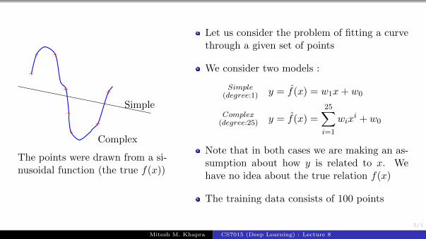
The points were drawn from a si-nusoidal function (the true f(x))
Let us consider the problem of fitting a curvethrough a given set of points
We consider two models :
Simple(degree:1) y = f(x) = w1x+ w0
Complex(degree:25) y = f(x) =
25∑i=1
wixi + w0
Note that in both cases we are making an as-sumption about how y is related to x. Wehave no idea about the true relation f(x)
The training data consists of 100 points
Mitesh M. Khapra CS7015 (Deep Learning) : Lecture 8

6/1
Simple
Complex
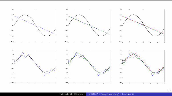
The points were drawn froma sinusoidal function (the truef(x))
We sample 25 points from the training dataand train a simple and a complex model
We repeat the process ‘k’ times to trainmultiple models (each model sees a differentsample of the training data)
We make a few observations from these plots
Mitesh M. Khapra CS7015 (Deep Learning) : Lecture 8
7/1
Mitesh M. Khapra CS7015 (Deep Learning) : Lecture 8

8/1
Simple models trained on different samples ofthe data do not differ much from each other
However they are very far from the true sinus-oidal curve (under fitting)
On the other hand, complex models trained ondifferent samples of the data are very differentfrom each other (high variance)
Mitesh M. Khapra CS7015 (Deep Learning) : Lecture 8
9/1
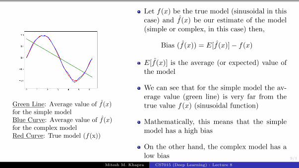
Green Line: Average value of f(x)for the simple modelBlue Curve: Average value of f(x)for the complex modelRed Curve: True model (f(x))
Let f(x) be the true model (sinusoidal in thiscase) and f(x) be our estimate of the model(simple or complex, in this case) then,
Bias (f(x)) = E[f(x)]− f(x)
E[f(x)] is the average (or expected) value ofthe model
We can see that for the simple model the av-erage value (green line) is very far from thetrue value f(x) (sinusoidal function)
Mathematically, this means that the simplemodel has a high bias
On the other hand, the complex model has alow bias
Mitesh M. Khapra CS7015 (Deep Learning) : Lecture 8

10/1
We now define,
Variance (f(x)) = E[(f(x)− E[f(x)])2]
(Standard definition from statistics)
Roughly speaking it tells us how much the dif-ferent f(x)’s (trained on different samples ofthe data) differ from each other
It is clear that the simple model has a low vari-ance whereas the complex model has a highvariance
Mitesh M. Khapra CS7015 (Deep Learning) : Lecture 8

11/1
In summary (informally)
Simple model: high bias, low variance
Complex model: low bias, high variance
There is always a trade-off between the biasand variance
Both bias and variance contribute to the meansquare error. Let us see how
Mitesh M. Khapra CS7015 (Deep Learning) : Lecture 8

12/1
Module 8.2 : Train error vs Test error
Mitesh M. Khapra CS7015 (Deep Learning) : Lecture 8
13/1
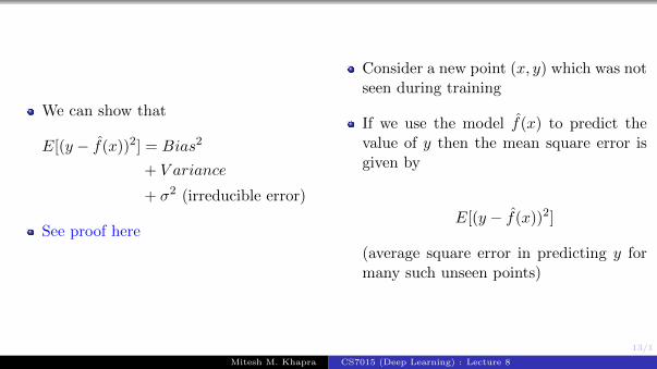
We can show that
E[(y − f(x))2] = Bias2
+ V ariance
+ σ2 (irreducible error)
See proof here
Consider a new point (x, y) which was notseen during training
If we use the model f(x) to predict thevalue of y then the mean square error isgiven by
E[(y − f(x))2]
(average square error in predicting y formany such unseen points)
Mitesh M. Khapra CS7015 (Deep Learning) : Lecture 8

14/1
model complexity
erro
r High bias High variance
Sweet spot--perfect tradeoff-ideal modelcomplexity
E[(y − f(x))2] = Bias2
+ V ariance
+ σ2 (irreducible error)
The parameters of f(x) (all wi’s) are trainedusing a training set (xi, yi)ni=1
However, at test time we are interested in eval-uating the model on a validation (unseen) setwhich was not used for training
This gives rise to the following two entities ofinterest:trainerr (say, mean square error)testerr (say, mean square error)
Typically these errors exhibit the trend shownin the adjacent figure
Mitesh M. Khapra CS7015 (Deep Learning) : Lecture 8
15/1
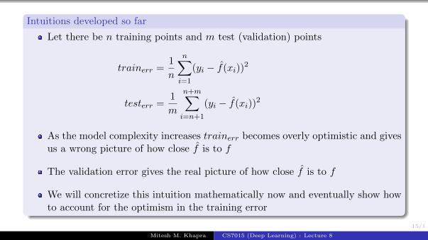
Intuitions developed so far
Let there be n training points and m test (validation) points
trainerr =1
n
n∑i=1
(yi − f(xi))2
testerr =1
m
n+m∑i=n+1
(yi − f(xi))2
As the model complexity increases trainerr becomes overly optimistic and givesus a wrong picture of how close f is to f
The validation error gives the real picture of how close f is to f
We will concretize this intuition mathematically now and eventually show howto account for the optimism in the training error
Mitesh M. Khapra CS7015 (Deep Learning) : Lecture 8
16/1
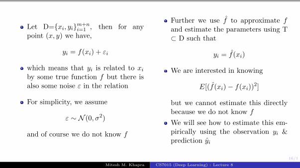
Let D=xi, yim+ni=1 , then for any
point (x, y) we have,
yi = f(xi) + εi
which means that yi is related to xiby some true function f but there isalso some noise ε in the relation
For simplicity, we assume
ε ∼ N (0, σ2)
and of course we do not know f
Further we use f to approximate fand estimate the parameters using T⊂ D such that
yi = f(xi)
We are interested in knowing
E[(f(xi)− f(xi))2]
but we cannot estimate this directlybecause we do not know f
We will see how to estimate this em-pirically using the observation yi &prediction yi
Mitesh M. Khapra CS7015 (Deep Learning) : Lecture 8

17/1
E[(yi − yi)2] = E[(f(xi)− f(xi)− εi)2] (yi = f(xi) + εi)
= E[(f(xi)− f(xi))2 − 2εi(f(xi)− f(xi)) + ε2i ]
= E[(f(xi)− f(xi))2]− 2E[εi(f(xi)− f(xi))] + E[ε2i ]
∴ E[(f(xi)− f(xi))2] = E[(yi − yi)2] − E[ε2i ] + 2E[ εi(f(xi)− f(xi)) ]
Mitesh M. Khapra CS7015 (Deep Learning) : Lecture 8

18/1
We will take a small detour to understand how to empirically estimate anExpectation and then return to our derivation
Mitesh M. Khapra CS7015 (Deep Learning) : Lecture 8
19/1
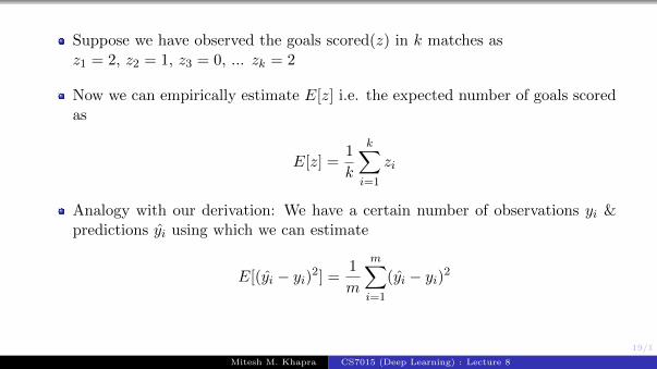
Suppose we have observed the goals scored(z) in k matches asz1 = 2, z2 = 1, z3 = 0, ... zk = 2
Now we can empirically estimate E[z] i.e. the expected number of goals scoredas
E[z] =1
k
k∑i=1
zi
Analogy with our derivation: We have a certain number of observations yi &predictions yi using which we can estimate
E[(yi − yi)2] =1
m
m∑i=1
(yi − yi)2
Mitesh M. Khapra CS7015 (Deep Learning) : Lecture 8

20/1
... returning back to our derivation
Mitesh M. Khapra CS7015 (Deep Learning) : Lecture 8

21/1
E[(f(xi)− f(xi))2] = E[(yi − yi)2] − E[ε2i ] + 2E[ εi(f(xi)− f(xi)) ]
We can empirically evaluate R.H.S using training observations or test observa-tions
Case 1: Using test observations
E[(f(xi)− f(xi))2]︸ ︷︷ ︸
true error
=1
m
n+m∑i=n+1
(yi − yi)2︸ ︷︷ ︸empirical estimation of error
− 1
m
n+m∑i=n+1
ε2i︸ ︷︷ ︸small constant
+ 2 E[ εi(f(xi)− f(xi)) ]︸ ︷︷ ︸= covariance (εi,f(xi)−f(xi))
∵ covariance(X,Y ) = E[(X − µX)(Y − µY )]
= E[(X)(Y − µY )](if µX = E[X] = 0)
= E[XY ]− E[XµY ] = E[XY ]− µYE[X] = E[XY ]
Mitesh M. Khapra CS7015 (Deep Learning) : Lecture 8
22/1
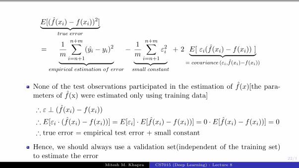
E[(f(xi)− f(xi))2]︸ ︷︷ ︸
true error
=1
m
n+m∑i=n+1
(yi − yi)2︸ ︷︷ ︸empirical estimation of error
− 1
m
n+m∑i=n+1
ε2i︸ ︷︷ ︸small constant
+ 2 E[ εi(f(xi)− f(xi)) ]︸ ︷︷ ︸= covariance (εi,f(xi)−f(xi))
None of the test observations participated in the estimation of f(x)[the para-meters of f(x) were estimated only using training data]
∴ ε ⊥ (f(xi)− f(xi))
∴ E[εi · (f(xi)− f(xi))] = E[εi] · E[f(xi)− f(xi))] = 0 · E[f(xi)− f(xi))] = 0
∴ true error = empirical test error + small constant
Hence, we should always use a validation set(independent of the training set)to estimate the error
Mitesh M. Khapra CS7015 (Deep Learning) : Lecture 8

23/1
Case 2: Using training observations
E[(f(xi)− f(xi))2]︸ ︷︷ ︸
true error
=1
n
n∑i=1
(yi − yi)2︸ ︷︷ ︸empirical estimation of error
− 1
n
n∑i=1
ε2i︸ ︷︷ ︸small constant
+ 2 E[ εi(f(xi)− f(xi)) ]︸ ︷︷ ︸= covariance (εi,f(xi)−f(xi))
Now, ε 6⊥ f(x) because ε was used for estimating the parameters of f(x)
∴ E[εi · (f(xi)− f(xi))] 6= E[εi] · E[f(xi)− f(xi))] 6= 0
Hence, the empirical train error is smaller than the true error and does not givea true picture of the error
But how is this related to model complexity? Let us see
Mitesh M. Khapra CS7015 (Deep Learning) : Lecture 8

24/1
Module 8.3 : True error and Model complexity
Mitesh M. Khapra CS7015 (Deep Learning) : Lecture 8

25/1
Using Stein’s Lemma (and some trickery) we can show that
1
n
n∑i=1
εi(f(xi)− f(xi)) =σ2
n
n∑i=1
∂f(xi)
∂yi
When will ∂f(xi)∂yi
be high? When a small change in the observation causes a
large change in the estimation(f)
Can you link this to model complexity?
Yes, indeed a complex model will be more sensitive to changes in observationswhereas a simple model will be less sensitive to changes in observations
Hence, we can say thattrue error = empirical train error + small constant + Ω(model complexity)
Mitesh M. Khapra CS7015 (Deep Learning) : Lecture 8

26/1
Mitesh M. Khapra CS7015 (Deep Learning) : Lecture 8

27/1
Let us verify that indeed acomplex model is more sens-itive to minor changes in thedata
We have fitted a simpleand complex model for somegiven data
We now change one of thesedata points
The simple model does notchange much as compared tothe complex model
Mitesh M. Khapra CS7015 (Deep Learning) : Lecture 8
28/1
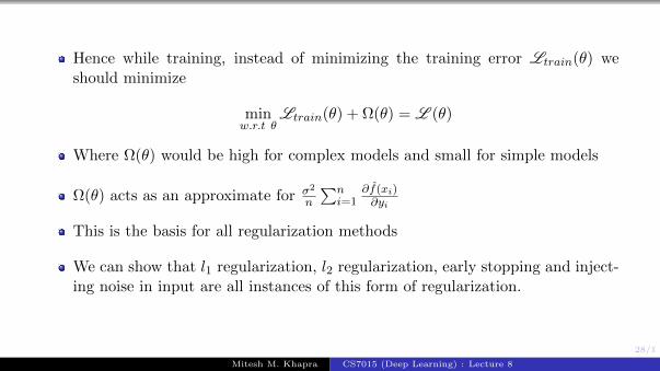
Hence while training, instead of minimizing the training error Ltrain(θ) weshould minimize
minw.r.t θ
Ltrain(θ) + Ω(θ) = L (θ)
Where Ω(θ) would be high for complex models and small for simple models
Ω(θ) acts as an approximate for σ2
n
∑ni=1
∂f(xi)∂yi
This is the basis for all regularization methods
We can show that l1 regularization, l2 regularization, early stopping and inject-ing noise in input are all instances of this form of regularization.
Mitesh M. Khapra CS7015 (Deep Learning) : Lecture 8
29/1
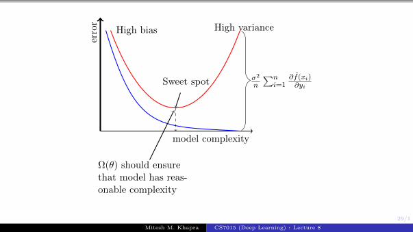
model complexity
erro
r
High bias High variance
Sweet spot
Ω(θ) should ensurethat model has reas-onable complexity
σ2
n
∑ni=1
∂f(xi)∂yi
Mitesh M. Khapra CS7015 (Deep Learning) : Lecture 8

30/1
Why do we care about thisbias variance tradeoff andmodel complexity?
Deep Neural networks are highly complexmodels.
Many parameters, many non-linearities.
It is easy for them to overfit and drive trainingerror to 0.
Hence we need some form of regularization.
Mitesh M. Khapra CS7015 (Deep Learning) : Lecture 8

31/1
Different forms of regularization
l2 regularization
Dataset augmentation
Parameter Sharing and tying
Adding Noise to the inputs
Adding Noise to the outputs
Early stopping
Ensemble methods
Dropout
Mitesh M. Khapra CS7015 (Deep Learning) : Lecture 8

32/1
Module 8.4 : l2 regularization
Mitesh M. Khapra CS7015 (Deep Learning) : Lecture 8

33/1
Different forms of regularization
l2 regularization
Dataset augmentation
Parameter Sharing and tying
Adding Noise to the inputs
Adding Noise to the outputs
Early stopping
Ensemble methods
Dropout
Mitesh M. Khapra CS7015 (Deep Learning) : Lecture 8
34/1
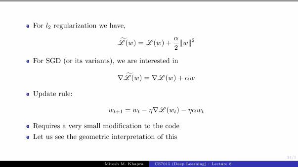
For l2 regularization we have,
L (w) = L (w) +α
2‖w‖2
For SGD (or its variants), we are interested in
∇L (w) = ∇L (w) + αw
Update rule:
wt+1 = wt − η∇L (wt)− ηαwt
Requires a very small modification to the code
Let us see the geometric interpretation of this
Mitesh M. Khapra CS7015 (Deep Learning) : Lecture 8
35/1
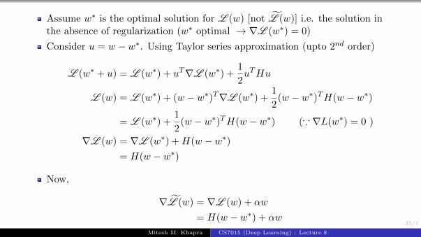
Assume w∗ is the optimal solution for L (w) [not L (w)] i.e. the solution inthe absence of regularization (w∗ optimal → ∇L (w∗) = 0)
Consider u = w − w∗. Using Taylor series approximation (upto 2nd order)
L (w∗ + u) = L (w∗) + uT∇L (w∗) +1
2uTHu
L (w) = L (w∗) + (w − w∗)T∇L (w∗) +1
2(w − w∗)TH(w − w∗)
= L (w∗) +1
2(w − w∗)TH(w − w∗) (∵ ∇L(w∗) = 0 )
∇L (w) = ∇L (w∗) +H(w − w∗)= H(w − w∗)
Now,
∇L (w) = ∇L (w) + αw
= H(w − w∗) + αw
Mitesh M. Khapra CS7015 (Deep Learning) : Lecture 8
36/1
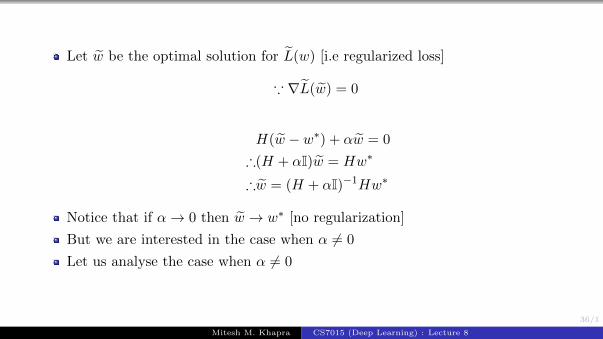
Let w be the optimal solution for L(w) [i.e regularized loss]
∵ ∇L(w) = 0
H(w − w∗) + αw = 0
∴(H + αI)w = Hw∗
∴w = (H + αI)−1Hw∗
Notice that if α→ 0 then w → w∗ [no regularization]
But we are interested in the case when α 6= 0
Let us analyse the case when α 6= 0
Mitesh M. Khapra CS7015 (Deep Learning) : Lecture 8
37/1
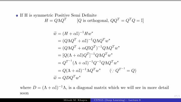
If H is symmetric Positive Semi DefiniteH = QΛQT [Q is orthogonal, QQT = QTQ = I]
w = (H + αI)−1Hw∗
= (QΛQT + αI)−1QΛQTw∗
= (QΛQT + αQIQT )−1QΛQTw∗
= [Q(Λ + αI)QT ]−1QΛQTw∗
= QT−1
(Λ + αI)−1Q−1QΛQTw∗
= Q(Λ + αI)−1ΛQTw∗ (∵ QT−1
= Q)
w = QDQTw∗
where D = (Λ + αI)−1Λ, is a diagonal matrix which we will see in more detailsoon
Mitesh M. Khapra CS7015 (Deep Learning) : Lecture 8

38/1
w = Q(Λ + αI)−1ΛQTw∗
= QDQTw∗
(Λ + αI)−1 =
1
λ1+α1
λ2+α. . .
1λn+α
D = (Λ + αI)−1Λ
(Λ + αI)−1Λ =
λ1
λ1+αλ2
λ2+α. . .
λnλn+α
So what is happening here?
w∗ first gets rotated by QT to giveQTw∗
However if α = 0 then Q rotatesQTw∗ back to give w∗
If α 6= 0 then let us see what Dlooks like
So what is happening now?
Mitesh M. Khapra CS7015 (Deep Learning) : Lecture 8
39/1
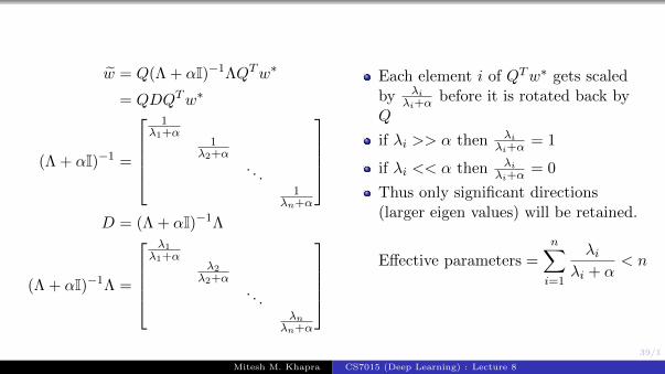
w = Q(Λ + αI)−1ΛQTw∗
= QDQTw∗
(Λ + αI)−1 =
1
λ1+α1
λ2+α. . .
1λn+α
D = (Λ + αI)−1Λ
(Λ + αI)−1Λ =
λ1
λ1+αλ2
λ2+α. . .
λnλn+α
Each element i of QTw∗ gets scaledby λi
λi+αbefore it is rotated back by
Q
if λi >> α then λiλi+α
= 1
if λi << α then λiλi+α
= 0
Thus only significant directions(larger eigen values) will be retained.
Effective parameters =
n∑i=1
λiλi + α
< n
Mitesh M. Khapra CS7015 (Deep Learning) : Lecture 8

40/1
The weight vector(w∗) is getting rotated to (w)
All of its elements are shrinking but some are shrinking more than the others
This ensures that only important features are given high weights
Mitesh M. Khapra CS7015 (Deep Learning) : Lecture 8

41/1
Module 8.5 : Dataset augmentation
Mitesh M. Khapra CS7015 (Deep Learning) : Lecture 8

42/1
Different forms of regularization
l2 regularization
Dataset augmentation
Parameter Sharing and tying
Adding Noise to the inputs
Adding Noise to the outputs
Early stopping
Ensemble methods
Dropout
Mitesh M. Khapra CS7015 (Deep Learning) : Lecture 8
43/1
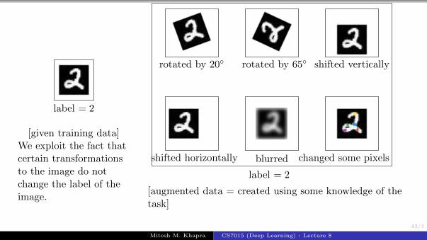
label = 2
[given training data]We exploit the fact thatcertain transformationsto the image do notchange the label of theimage.
label = 2
rotated by 20 rotated by 65 shifted vertically
shifted horizontally blurred changed some pixels
[augmented data = created using some knowledge of thetask]
Mitesh M. Khapra CS7015 (Deep Learning) : Lecture 8

44/1
Typically, More data = better learning
Works well for image classification / object recognition tasks
Also shown to work well for speech
For some tasks it may not be clear how to generate such data
Mitesh M. Khapra CS7015 (Deep Learning) : Lecture 8

45/1
Module 8.6 : Parameter Sharing and tying
Mitesh M. Khapra CS7015 (Deep Learning) : Lecture 8

46/1
Other forms of regularization
l2 regularization
Dataset augmentation
Parameter Sharing and tying
Adding Noise to the inputs
Adding Noise to the outputs
Early stopping
Ensemble methods
Dropout
Mitesh M. Khapra CS7015 (Deep Learning) : Lecture 8
47/1
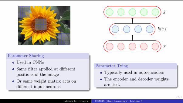
Parameter Sharing
Used in CNNs
Same filter applied at differentpositions of the image
Or same weight matrix acts ondifferent input neurons
x
h(x)
x
Parameter Tying
Typically used in autoencoders
The encoder and decoder weightsare tied.
Mitesh M. Khapra CS7015 (Deep Learning) : Lecture 8
48/1
Module 8.7 : Adding Noise to the inputs
Mitesh M. Khapra CS7015 (Deep Learning) : Lecture 8

49/1
Other forms of regularization
l2 regularization
Dataset augmentation
Parameter Sharing and tying
Adding Noise to the inputs
Adding Noise to the outputs
Early stopping
Ensemble methods
Dropout
Mitesh M. Khapra CS7015 (Deep Learning) : Lecture 8
50/1
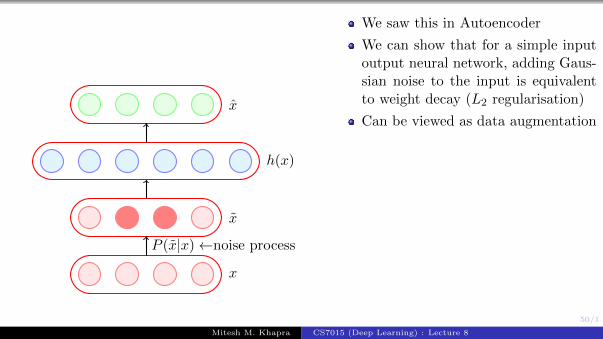
x
x
h(x)
x
P (x|x)←noise process
We saw this in Autoencoder
We can show that for a simple inputoutput neural network, adding Gaus-sian noise to the input is equivalentto weight decay (L2 regularisation)
Can be viewed as data augmentation
Mitesh M. Khapra CS7015 (Deep Learning) : Lecture 8

51/1
x1 + ε1 x2 + ε2
. . .xk + εk
. . .xn + εn
ε ∼ N (0, σ2)
xi = xi + εi
y =
n∑i=1
wixi
y =
n∑i=1
wixi
=
n∑i=1
wixi +
n∑i=1
wiεi
= y +
n∑i=1
wiεi
We are interested in E[(y − y)2]
E[(y − y)2
]= E
[(y +
n∑i=1
wiεi − y)2]
= E
((y − y)+( n∑
i=1
wiεi
))2
= E[(y − y)2
]+ E
[2(y − y)
n∑i=1
wiεi
]+ E
[( n∑i=1
wiεi
)2]
= E[(y − y)2
]+ 0 + E
[n∑
i=1
w2i ε
2i
](∵ εi is independent of εj and εi is independent of (y-y) )
= (E[(y − y)2
]+ σ2
n∑i=1
w2i (same as L2 norm penalty)
Mitesh M. Khapra CS7015 (Deep Learning) : Lecture 8
52/1
Module 8.8 : Adding Noise to the outputs
Mitesh M. Khapra CS7015 (Deep Learning) : Lecture 8

53/1
Other forms of regularization
l2 regularization
Dataset augmentation
Parameter Sharing and tying
Adding Noise to the inputs
Adding Noise to the outputs
Early stopping
Ensemble methods
Dropout
Mitesh M. Khapra CS7015 (Deep Learning) : Lecture 8
54/1
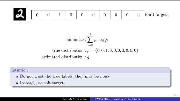
Hard targets0 0 1 0 0 0 0 0 0 0
minimize :
9∑i=0
pi log qi
true distribution : p = 0, 0, 1, 0, 0, 0, 0, 0, 0, 0estimated distribution : q
Intuition
Do not trust the true labels, they may be noisy
Instead, use soft targets
Mitesh M. Khapra CS7015 (Deep Learning) : Lecture 8
55/1
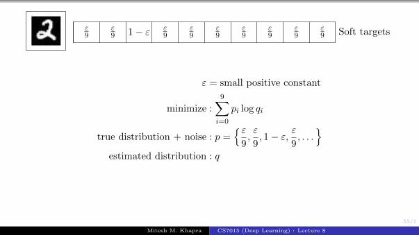
Soft targetsε9
ε9 1− ε ε
9ε9
ε9
ε9
ε9
ε9
ε9
ε = small positive constant
minimize :
9∑i=0
pi log qi
true distribution + noise : p =ε
9,ε
9, 1− ε, ε
9, . . .
estimated distribution : q
Mitesh M. Khapra CS7015 (Deep Learning) : Lecture 8

56/1
Module 8.9 : Early stopping
Mitesh M. Khapra CS7015 (Deep Learning) : Lecture 8

57/1
Other forms of regularization
l2 regularization
Dataset augmentation
Parameter Sharing and tying
Adding Noise to the inputs
Adding Noise to the outputs
Early stopping
Ensemble methods
Dropout
Mitesh M. Khapra CS7015 (Deep Learning) : Lecture 8
58/1
Steps
Error
Training error
V alidation error
k − p kstopreturn this model
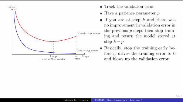
Track the validation error
Have a patience parameter p
If you are at step k and there wasno improvement in validation error inthe previous p steps then stop train-ing and return the model stored atstep k − pBasically, stop the training early be-fore it drives the training error to 0and blows up the validation error
Mitesh M. Khapra CS7015 (Deep Learning) : Lecture 8
59/1
Steps
Error
Training error
V alidation error
k − p kstopreturn this model
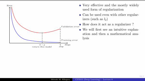
Very effective and the mostly widelyused form of regularization
Can be used even with other regular-izers (such as l2)
How does it act as a regularizer ?
We will first see an intuitive explan-ation and then a mathematical ana-lysis
Mitesh M. Khapra CS7015 (Deep Learning) : Lecture 8

60/1
Steps
Error
Training error
V alidation error
k − p kstopreturn this model
Recall that the update rule in SGD is
wt+1 = wt − η∇wt
= w0 − ηt∑i=1
∇wi
Let τ be the maximum value of ∇withen
|wt+1 − w0| ≤ ηt|τ |
Thus, t controls how far wt can gofrom the initial w0
In other words it controls the spaceof exploration
Mitesh M. Khapra CS7015 (Deep Learning) : Lecture 8

61/1
We will now see a mathematical analysis of this
Mitesh M. Khapra CS7015 (Deep Learning) : Lecture 8

62/1
Recall that the Taylor series approximation for L (w) is
L (w) = L (w∗) + (w − w∗)T∇L (w∗) +1
2(w − w∗)TH(w − w∗)
= L (w∗) +1
2(w − w∗)TH(w − w∗) [ w∗ is optimal so ∇L (w∗) is 0 ]
∇(L (w)) = H(w − w∗)
Now the SGD update rule is:
wt = wt−1 − η∇L (wt−1)
= wt−1 − ηH(wt−1 − w∗)= (I − ηH)wt−1 + ηHw∗
Mitesh M. Khapra CS7015 (Deep Learning) : Lecture 8
63/1
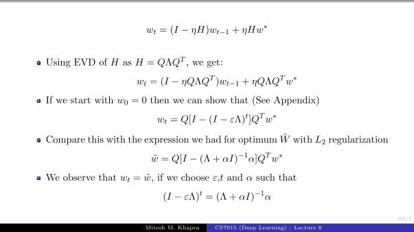
wt = (I − ηH)wt−1 + ηHw∗
Using EVD of H as H = QΛQT , we get:
wt = (I − ηQΛQT )wt−1 + ηQΛQTw∗
If we start with w0 = 0 then we can show that (See Appendix)
wt = Q[I − (I − εΛ)t]QTw∗
Compare this with the expression we had for optimum W with L2 regularization
w = Q[I − (Λ + αI)−1α]QTw∗
We observe that wt = w, if we choose ε,t and α such that
(I − εΛ)t = (Λ + αI)−1α
Mitesh M. Khapra CS7015 (Deep Learning) : Lecture 8
64/1
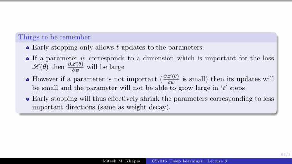
Things to be remember
Early stopping only allows t updates to the parameters.
If a parameter w corresponds to a dimension which is important for the lossL (θ) then ∂L (θ)
∂w will be large
However if a parameter is not important (∂L (θ)∂w is small) then its updates will
be small and the parameter will not be able to grow large in ‘t′ steps
Early stopping will thus effectively shrink the parameters corresponding to lessimportant directions (same as weight decay).
Mitesh M. Khapra CS7015 (Deep Learning) : Lecture 8

65/1
Module 8.10 : Ensemble methods
Mitesh M. Khapra CS7015 (Deep Learning) : Lecture 8

66/1
Other forms of regularization
l2 regularization
Dataset augmentation
Parameter Sharing and tying
Adding Noise to the inputs
Adding Noise to the outputs
Early stopping
Ensemble methods
Dropout
Mitesh M. Khapra CS7015 (Deep Learning) : Lecture 8
67/1
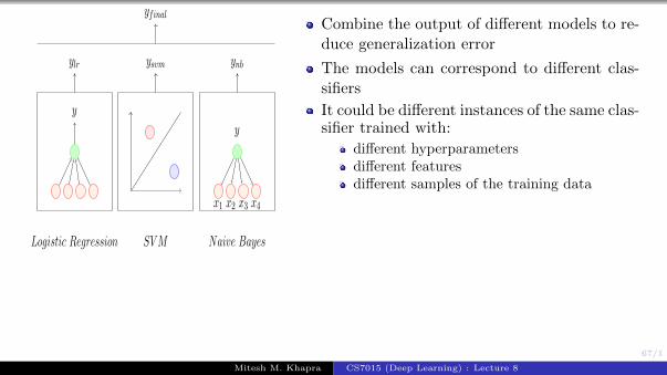
y
ylr
Logistic Regression
ysvm
SVM
ynb
x1 x2 x3 x4
y
Naive Bayes
yfinalCombine the output of different models to re-duce generalization error
The models can correspond to different clas-sifiers
It could be different instances of the same clas-sifier trained with:
different hyperparametersdifferent featuresdifferent samples of the training data
Mitesh M. Khapra CS7015 (Deep Learning) : Lecture 8

68/1
y
ylr1
y
ylr2
y
ylr3
Logistic LogisticLogisticRegression RegressionRegression
yfinal
Each model trained with a differentsample of the data (sampling withreplacement)
Bagging: form an ensemble using dif-ferent instances of the same classifier
From a given dataset, construct mul-tiple training sets by sampling withreplacement (T1, T2, ..., Tk)
Train ith instance of the classifier us-ing training set Ti
Mitesh M. Khapra CS7015 (Deep Learning) : Lecture 8
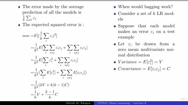
69/1
The error made by the averageprediction of all the models is1k
∑i εi
The expected squared error is :
mse =E[(1
k
∑i
εi)2]
=1
k2E[∑i
∑i=j
εiεj +∑i
∑i 6=j
εiεj ]
=1
k2E[∑i
ε2i +∑i
∑i 6=j
εiεj ]
=1
k2(∑i
E[ε2i ] +∑i
∑i 6=j
E[εiεj ])
=1
k2(kV + k(k − 1)C)
=1
kV +
k − 1
kC
When would bagging work?
Consider a set of k LR mod-els
Suppose that each modelmakes an error εi on a testexample
Let εi be drawn from azero mean multivariate nor-mal distribution
V ariance = E[ε2i ] = V
Covariance = E[εiεj ] = C
Mitesh M. Khapra CS7015 (Deep Learning) : Lecture 8

70/1
mse =1
kV +
k − 1
kC
When would bagging work ?
If the errors of the model are perfectlycorrelated then V = C and mse = V[bagging does not help: the mse of theensemble is as bad as the individualmodels]
If the errors of the model are inde-pendent or uncorrelated then C = 0and the mse of the ensemble reducesto 1
kV
On average, the ensemble will per-form at least as well as its individualmembers
Mitesh M. Khapra CS7015 (Deep Learning) : Lecture 8

71/1
Module 8.11 : Dropout
Mitesh M. Khapra CS7015 (Deep Learning) : Lecture 8

72/1
Other forms of regularization
l2 regularization
Dataset augmentation
Parameter Sharing and tying
Adding Noise to the inputs
Adding Noise to the outputs
Early stopping
Ensemble methods
Dropout
Mitesh M. Khapra CS7015 (Deep Learning) : Lecture 8

73/1
Typically model averaging(baggingensemble) always helps
Training several large neural net-works for making an ensemble is pro-hibitively expensive
Option 1: Train several neuralnetworks having different architec-tures(obviously expensive)
Option 2: Train multiple instancesof the same network using differenttraining samples (again expensive)
Even if we manage to train with op-tion 1 or option 2, combining severalmodels at test time is infeasible inreal time applications
Mitesh M. Khapra CS7015 (Deep Learning) : Lecture 8

74/1
Dropout is a technique which ad-dresses both these issues.
Effectively it allows training severalneural networks without any signific-ant computational overhead.
Also gives an efficient approximateway of combining exponentially manydifferent neural networks.
Mitesh M. Khapra CS7015 (Deep Learning) : Lecture 8

75/1
Dropout refers to dropping out units
Temporarily remove a node and all its incoming/outgoing connectionsresulting in a thinned network
Each node is retained with a fixed probability (typically p = 0.5) for hiddennodes and p = 0.8 for visible nodes
Mitesh M. Khapra CS7015 (Deep Learning) : Lecture 8
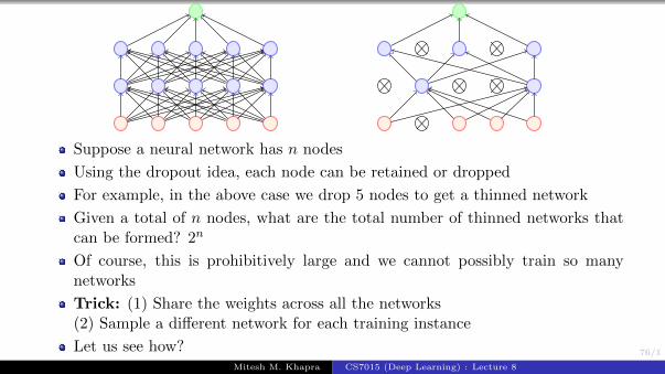
76/1
Suppose a neural network has n nodes
Using the dropout idea, each node can be retained or dropped
For example, in the above case we drop 5 nodes to get a thinned network
Given a total of n nodes, what are the total number of thinned networks thatcan be formed? 2n
Of course, this is prohibitively large and we cannot possibly train so manynetworks
Trick: (1) Share the weights across all the networks(2) Sample a different network for each training instance
Let us see how?Mitesh M. Khapra CS7015 (Deep Learning) : Lecture 8

77/1
We initialize all the parameters (weights) of the network and start training
For the first training instance (or mini-batch), we apply dropout resulting inthe thinned network
We compute the loss and backpropagate
Which parameters will we update? Only those which are active
Mitesh M. Khapra CS7015 (Deep Learning) : Lecture 8
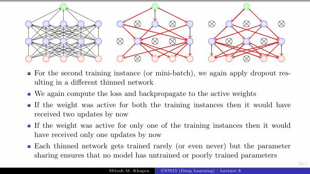
78/1
For the second training instance (or mini-batch), we again apply dropout res-ulting in a different thinned network
We again compute the loss and backpropagate to the active weights
If the weight was active for both the training instances then it would havereceived two updates by now
If the weight was active for only one of the training instances then it wouldhave received only one updates by now
Each thinned network gets trained rarely (or even never) but the parametersharing ensures that no model has untrained or poorly trained parameters
Mitesh M. Khapra CS7015 (Deep Learning) : Lecture 8

79/1
Present withprobability p
w1 w2 w3 w4
At training time
Alwayspresent
pw1 pw2 pw3 pw4
At test time
What happens at test time?
Impossible to aggregate the outputs of 2n thinned networks
Instead we use the full Neural Network and scale the output of each node bythe fraction of times it was on during training
Mitesh M. Khapra CS7015 (Deep Learning) : Lecture 8
80/1
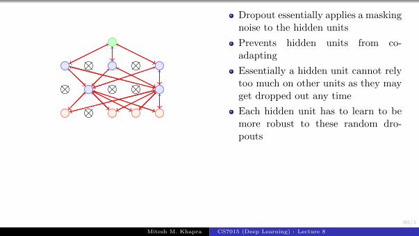
Dropout essentially applies a maskingnoise to the hidden units
Prevents hidden units from co-adapting
Essentially a hidden unit cannot relytoo much on other units as they mayget dropped out any time
Each hidden unit has to learn to bemore robust to these random dro-pouts
Mitesh M. Khapra CS7015 (Deep Learning) : Lecture 8
81/1
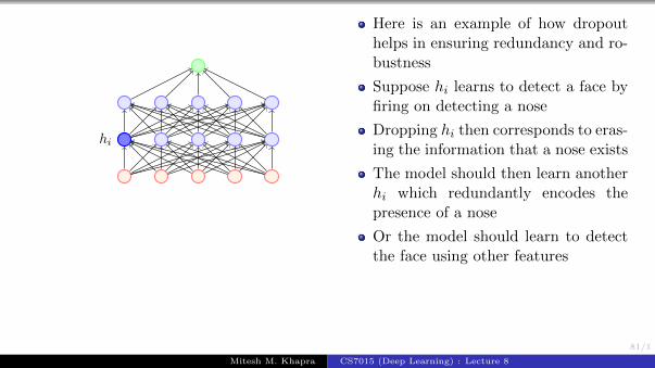
hi
Here is an example of how dropouthelps in ensuring redundancy and ro-bustness
Suppose hi learns to detect a face byfiring on detecting a nose
Dropping hi then corresponds to eras-ing the information that a nose exists
The model should then learn anotherhi which redundantly encodes thepresence of a nose
Or the model should learn to detectthe face using other features
Mitesh M. Khapra CS7015 (Deep Learning) : Lecture 8

82/1
Recap
l2 regularization
Dataset augmentation
Parameter Sharing and tying
Adding Noise to the inputs
Adding Noise to the outputs
Early stopping
Ensemble methods
Dropout
Mitesh M. Khapra CS7015 (Deep Learning) : Lecture 8

83/1
Appendix
Mitesh M. Khapra CS7015 (Deep Learning) : Lecture 8

84/1
To prove: The below two equations are equivalent
wt = (I − ηQΛQT )wt−1 + ηQΛQTw∗
wt = Q[I − (I − εΛ)t]QTw∗
Proof by induction:
Base case: t = 1 and w0=0:
w1 according to the first equation:
w1 = (I − ηQΛQT )w0 + ηQΛQTw∗
= ηQΛQTw∗
w1 according to the second equation:
w1 = Q(I − (I − ηΛ)1)QTw∗
= ηQΛQTw∗
Mitesh M. Khapra CS7015 (Deep Learning) : Lecture 8

85/1
Induction step: Let the two equations be equivalent for tth step
∴ wt = (I − ηQΛQT )wt−1 + ηQΛQTw∗
= Q[I − (I − εΛ)t]QTw∗
Proof that this will hold for (t+ 1)th step
wt+1 = (I − ηQΛQT )wt + ηQΛQTw∗
(using wt = Q[I − (I − εΛ)t]QTw∗)
(using wt = Q[I − (I − εΛ)t]QTw∗)
= (I − ηQΛQT )Q(I − (I − ηΛ)t)QTw∗ + ηQΛQTw∗
= (I − ηQΛQT )Q(I − (I − ηΛ)t)QTw∗ + ηQΛQTw∗
= (I − ηQΛQT )Q(I − (I − ηΛ)t)QTw∗ + ηQΛQTw∗
(Opening this bracket)
= IQ(I − (I − ηΛ)t)QTw∗ − ηQΛQTQ(I − (I − ηΛ)t)QTw∗ + ηQΛQTw∗
= Q(I − (I − ηΛ)t)QTw∗ − ηQΛQTQ(I − (I − ηΛ)t)QTw∗ + ηQΛQTw∗Mitesh M. Khapra CS7015 (Deep Learning) : Lecture 8
86/1
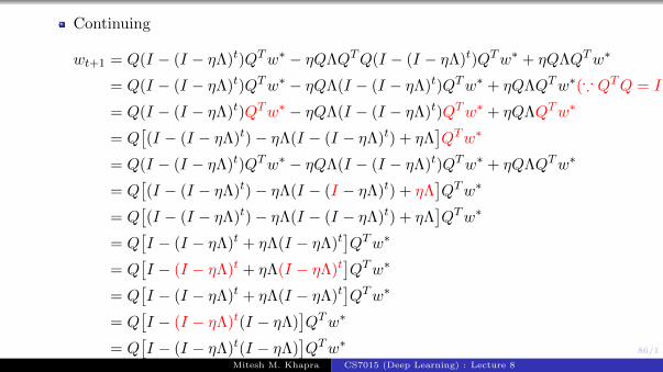
Continuing
wt+1 = Q(I − (I − ηΛ)t)QTw∗ − ηQΛQTQ(I − (I − ηΛ)t)QTw∗ + ηQΛQTw∗
= Q(I − (I − ηΛ)t)QTw∗ − ηQΛ(I − (I − ηΛ)t)QTw∗ + ηQΛQTw∗(∵ QTQ = I)
= Q(I − (I − ηΛ)t)QTw∗ − ηQΛ(I − (I − ηΛ)t)QTw∗ + ηQΛQTw∗
= Q[(I − (I − ηΛ)t)− ηΛ(I − (I − ηΛ)t) + ηΛ
]QTw∗
= Q(I − (I − ηΛ)t)QTw∗ − ηQΛ(I − (I − ηΛ)t)QTw∗ + ηQΛQTw∗
= Q[(I − (I − ηΛ)t)− ηΛ(I − (I − ηΛ)t) + ηΛ
]QTw∗
= Q[(I − (I − ηΛ)t)− ηΛ(I − (I − ηΛ)t) + ηΛ
]QTw∗
= Q[I − (I − ηΛ)t + ηΛ(I − ηΛ)t
]QTw∗
= Q[I − (I − ηΛ)t + ηΛ(I − ηΛ)t
]QTw∗
= Q[I − (I − ηΛ)t + ηΛ(I − ηΛ)t
]QTw∗
= Q[I − (I − ηΛ)t(I − ηΛ)
]QTw∗
= Q[I − (I − ηΛ)t(I − ηΛ)
]QTw∗
= Q(I − (I − ηΛ)t+1)QTw∗
Hence, proved!
Mitesh M. Khapra CS7015 (Deep Learning) : Lecture 8