CS5226

Indexing and Index Tuning

When Change is the Only Constant

CPUMemory Speed and SizeHarddisk Speed and SizeBandwidth

Moore’s Law being proved...

1969 2001 Factormain memory 200 KB 200 MB 103

cache 20 KB 20 MB 103

cache pages 20 5000 <103

disk size 7.5 MB 20 GB 3*103disk/memory size 40 100 -2.5transfer rate 150 KB/s 15 MB/s 102random access 50 ms 5 ms 10scanning full disk 130 s 1300 s -10

Improvement in Performance

1

10

100

1000

10000

1980 2000

CPU (60%/yr)

DRAM (10%/yr)

Disk(5%/yr)

Indexing

Single dimensional IndexingMulti-dimensional IndexingHigh-dimensional IndexingIndexing for advanced applications

Single Record and Range Searches

Single record retrievals ``Find student name whose matric# = 921000Y13’’

Range queries ``Find all students with cap > 3.0’’

Sequentially scanning the file is costly If data is in sorted file, do binary search to find

first such student, then scan to find others.cost of binary search can still be quite high.

Indexes

An index on a file speeds up selections on the search key fields for the index. Any subset of the fields of a relation can be the

search key for an index on the relation. Search key is not the same as key (minimal set

of fields that uniquely identify a record in a relation).

e.g., consider Student(matric#, name, addr, cap), the key is matric#, but the search key can be matric#, name, addr, cap or any combination of them.

Sequential File

2010

4030

6050

8070

10090

Dense Index

10203040

50607080

90100110120

Simple Index File (Data File Sorted)

Sequential File

2010

4030

6050

8070

10090

Sparse Index10305070

90110130150

170190210230

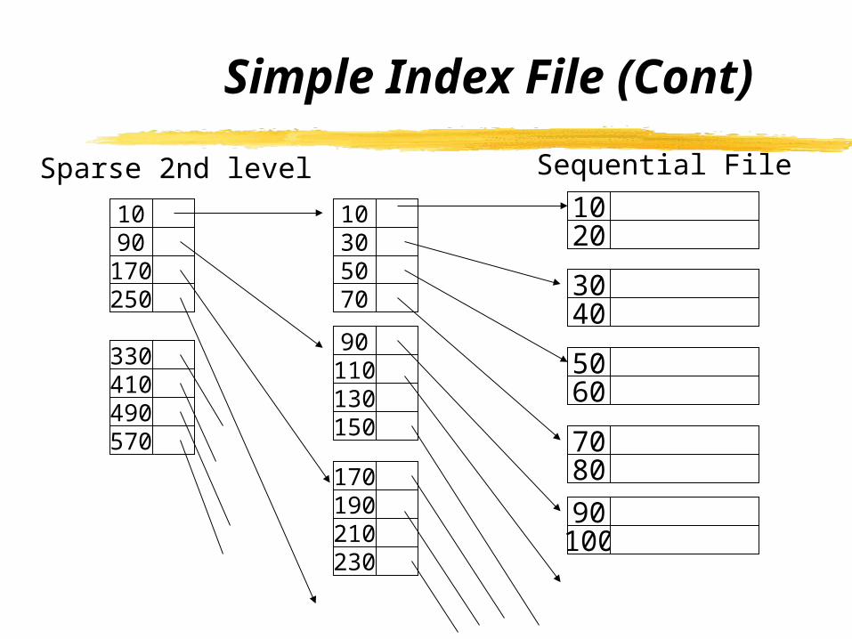
Simple Index File (Cont)

Sequential File

2010

4030

6050

8070

10090

Sparse 2nd level

10305070

90110130150

170190210230

1090

170250

330410490570

Simple Index File (Cont)

Secondary indexes

Sequencefield

5030

7020

4080

10100

6090

• Sparse index302080

100

90...

does not make sense!

Sequencefield

5030

7020

4080

10100

6090

• Dense index

10203040

506070...

105090...

sparsehighlevel

Secondary indexes

Conventional indexes

Advantages:- Simple- Index is sequential file

good for scans

Disadvantages:- Inserts expensive, and/or- Lose sequentiality & balance

102030

405060

708090

39313536

323834

33

overflow area(not sequential)

Example

Index(sequential)

continuous

free space

Tree-Structured Indexing

Tree-structured indexing techniques support both range searches and equality searches index file may still be quite large. But

we can apply the idea repeatedly!

Data pages

B+ Tree: The Most Widely Used Index

Height-balanced. Insert/delete at log F N cost (F = fanout, N = #

leaf pages);

Grow and shrink dynamically. Minimum 50% occupancy (except for root).

Each node contains d <= m <= 2d entries. The parameter d is called the order of the tree.

`next-leaf-pointer’ to chain up the leaf nodes.

Data entries at leaf are sorted.

Example B+ Tree

Each node can hold 4 entries (order = 2)

2 3

Root

17

24 30

14 16 19 20 22 24 27 29 33 34 38 39

135

75 8

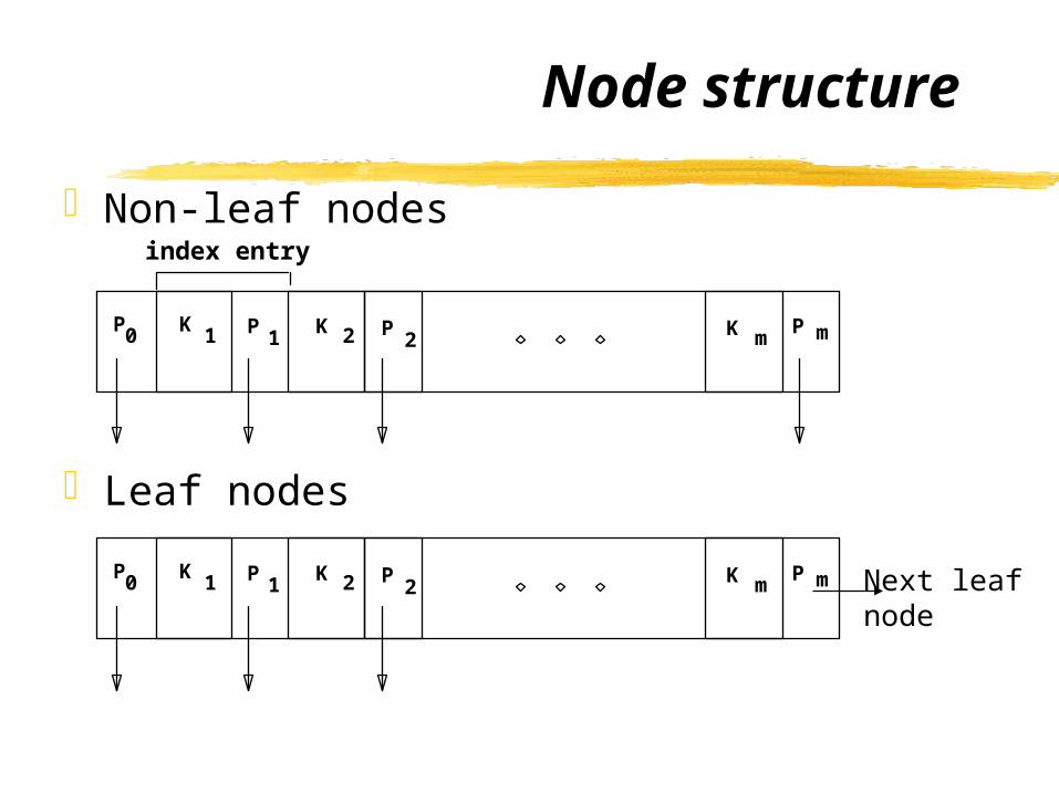
Node structure

P0

K1 P

1K 2 P

2K m

P m

index entry

Non-leaf nodes

Leaf nodes

P0

K1 P

1K 2 P

2K m

P m Next leaf node

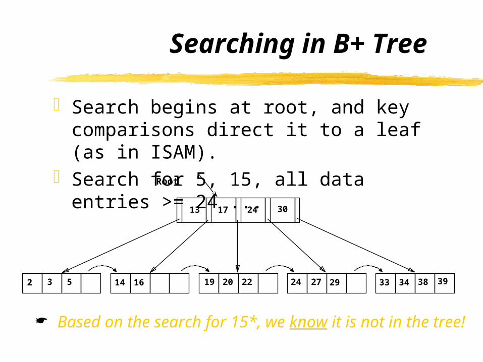
Searching in B+ Tree

Search begins at root, and key comparisons direct it to a leaf (as in ISAM).

Search for 5, 15, all data entries >= 24 ...

Based on the search for 15*, we know it is not in the tree!

Root

17 24 30

2 3 5 14 16 19 20 22 24 27 29 33 34 38 39

13

B+-Tree Scalability

Typical order: 100. Typical fill-factor: 67%. average fanout = 133

Typical capacities (root at Level 1, and has 133 entries): Level 5: 1334 = 312,900,700 records Level 4: 1333 = 2,352,637 records

Can often hold top levels in buffer pool: Level 1 = 1 page = 8 Kbytes Level 2 = 133 pages = 1 Mbyte Level 3 = 17,689 pages = 133 MBytes

A Note on `Order’

Order (d) concept replaced by physical space criterion in practice (`at least half-full’). Index pages can typically hold many more entries

than leaf pages. Variable sized records and search keys mean

different nodes will contain different numbers of entries.

Even with fixed length fields, multiple records with the same search key value (duplicates) can lead to variable-sized data entries

Inserting a Data Entry into a B+ TreeFind correct leaf L. Put data entry onto L.

If L has enough space, done! Else, must split L (into L and a new node L2)

Redistribute entries evenly, copy up middle key.Insert index entry pointing to L2 into parent of L.

This can happen recursively To split index node, redistribute entries evenly, but

push up middle key. (Contrast with leaf splits.)

Splits “grow” tree; root split increases height. Tree growth: gets wider or one level taller at top.

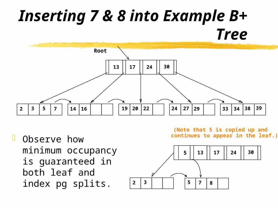
Inserting 7 & 8 into Example B+ Tree

Root

2 3 5 7 14 16 19 20 22 24 27 29 33 34 38 39

2 3 5 7 8

5

(Note that 5 is copied up andcontinues to appear in the leaf.)

17 24 3013

17 24 3013

Observe how minimum occupancy is guaranteed in both leaf and index pg splits.

Insertion (Cont)

Note difference between copy-up and push-up; be sure you understand the reasons for this.

appears once in the index. Contrast

5 24 30

17

13

(Note that 17 is pushed up and only

this with a leaf split.)

2 3 5 7 8

5 17 24 3013

Example B+ Tree After Inserting 8

Notice that root was split, leading to increase in height.

In this example, we can avoid splitting by re-distributing entries; however, this is usually not done in practice. Why?

2 3

Root

17

24 30

14 16 19 20 22 24 27 29 33 34 38 39

135

75 8

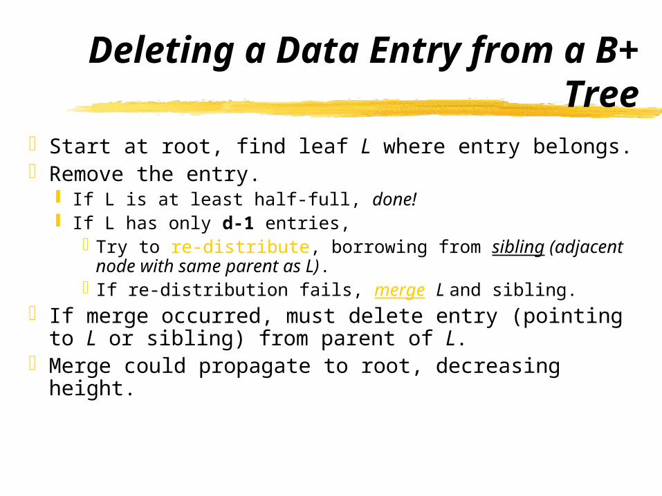
Deleting a Data Entry from a B+ Tree

Start at root, find leaf L where entry belongs.Remove the entry.

If L is at least half-full, done! If L has only d-1 entries,

Try to re-distribute, borrowing from sibling (adjacent node with same parent as L).

If re-distribution fails, merge L and sibling. If merge occurred, must delete entry (pointing to

L or sibling) from parent of L.Merge could propagate to root, decreasing

height.

Example Tree After (Inserting 8, Then) Deleting 19

Deleting 19 is easy.

2 3

Root

17

24 30

14 16 20 22 24 27 29 33 34 38 39

135

75 8

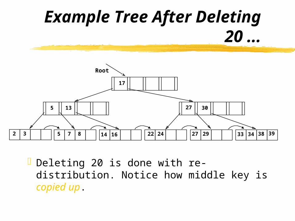
Example Tree After Deleting 20 ...

Deleting 20 is done with re-distribution. Notice how middle key is copied up.

2 3

Root

17

30

14 16 33 34 38 39

135

75 8 22 24

27

27 29

... And Then Deleting 24

Must merge.Observe `toss’ of

index entry (on right), and `pull down’ of index entry (below).

30

22 27 29 33 34 38 39

2 3 7 14 16 22 27 29 33 34 38 395 8

Root30135 17

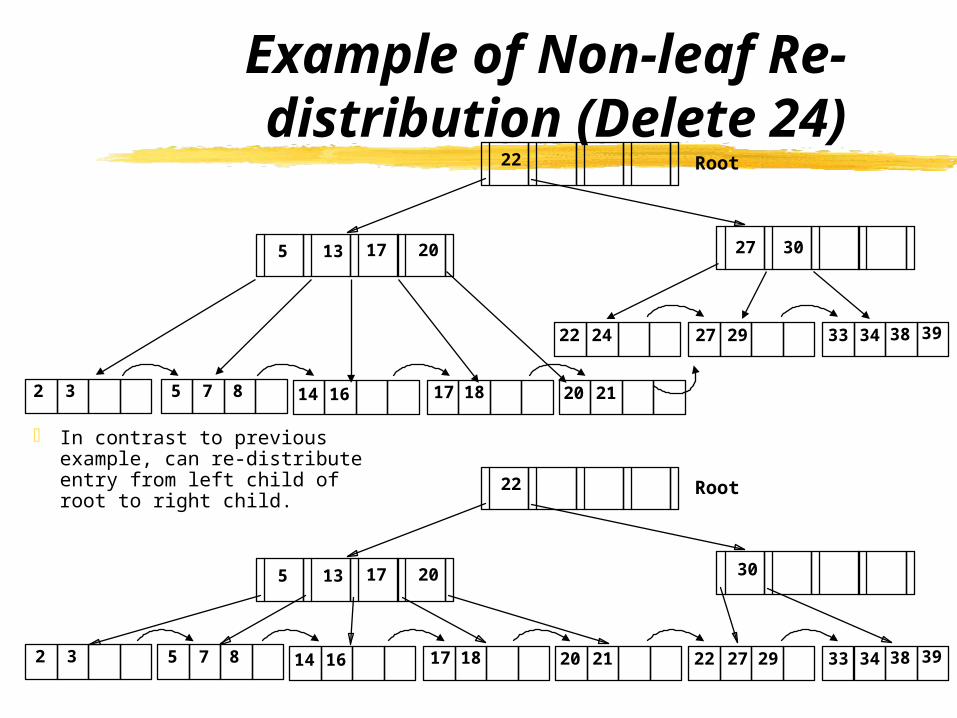
Example of Non-leaf Re-distribution (Delete 24)

In contrast to previous example, can re-distribute entry from left child of root to right child.

Root

135 17 20

22

30

14 16 17 18 20 33 34 38 3922 27 292175 832

Root

135 17 20

22

30

14 16 17 18 20

33 34 38 3927 29

2175 832

22 24

27

After Re-distribution

Intuitively, entries are re-distributed by `pushing through’ the splitting entry in the parent node.

It suffices to re-distribute index entry with key 20; we’ve re-distributed 17 as well for illustration.

14 16 33 34 38 3922 27 2917 18 20 2175 82 3

Root

135

17

3020 22

Index Classification

Primary vs. secondary: If search key contains primary key, then called primary index. Unique index: Search key contains a candidate key.

Clustered vs. unclustered: If order of data records is the same as, or `close to’, order of data entries, then called clustered index. A file can be clustered on at most one search key. Cost of retrieving data records through index varies

greatly based on whether index is clustered or not!

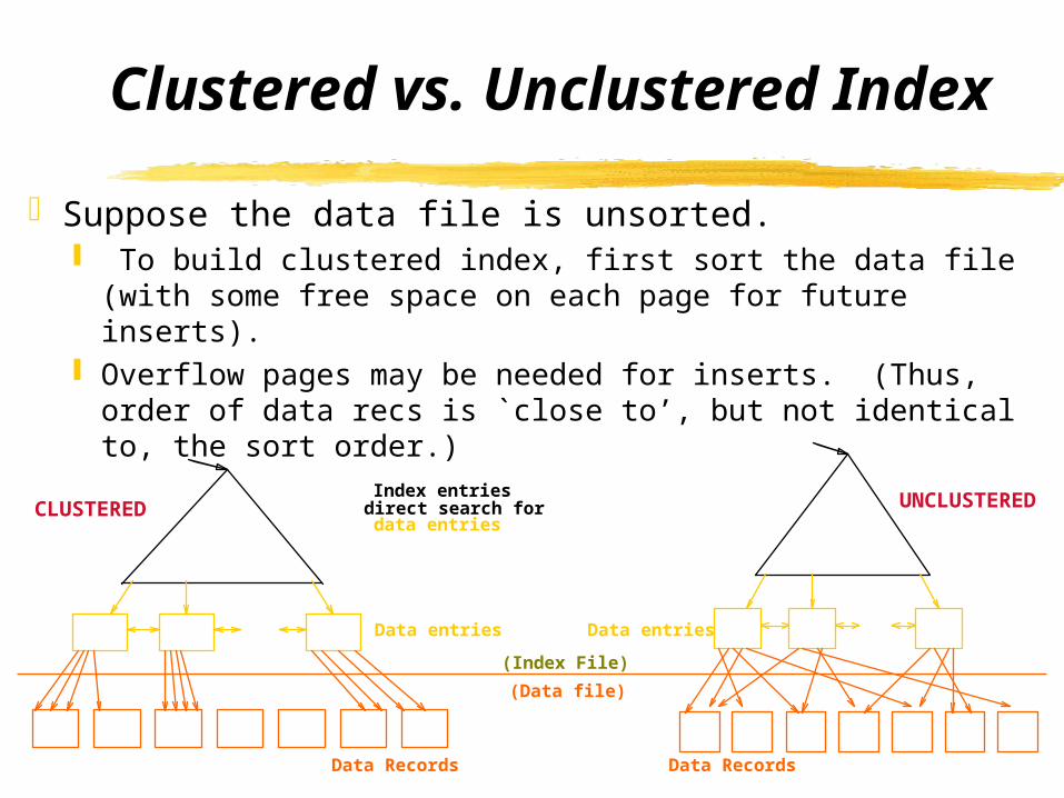
Clustered vs. Unclustered Index

Suppose the data file is unsorted. To build clustered index, first sort the data file (with

some free space on each page for future inserts). Overflow pages may be needed for inserts. (Thus,

order of data recs is `close to’, but not identical to, the sort order.)

Index entries

Data entries

direct search for

(Index File)

(Data file)

Data Records

data entries

Data entries

Data Records

CLUSTERED UNCLUSTERED

Index Classification (Cont.)

Dense vs. Sparse: If there is at least one data entry per search key value (in some data record), then dense. Every sparse

index is clustered! Sparse indexes

are smaller.

Ashby, 25, 3000

Smith, 44, 3000

Ashby

Cass

Smith

22

25

30

40

44

44

50

Sparse Indexon

Name Data File

Dense Indexon

Age

33

Bristow, 30, 2007

Basu, 33, 4003

Cass, 50, 5004

Tracy, 44, 5004

Daniels, 22, 6003

Jones, 40, 6003

Index Classification (Cont.)

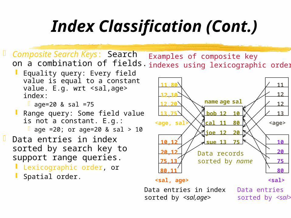
Composite Search Keys: Search on a combination of fields. Equality query: Every field value

is equal to a constant value. E.g. wrt <sal,age> index:

age=20 & sal =75 Range query: Some field value

is not a constant. E.g.: age =20; or age=20 & sal > 10

Data entries in index sorted by search key to support range queries. Lexicographic order, or Spatial order.

sue 13 75

bob

cal

joe 12

10

20

8011

12

name age sal

<sal, age>

<age, sal> <age>

<sal>

12,20

12,10

11,80

13,75

20,12

10,12

75,13

80,11

11

12

12

13

10

20

75

80

Data recordssorted by name

Data entries in indexsorted by <sal,age>

Data entriessorted by <sal>

Examples of composite keyindexes using lexicographic order.

Summary

Tree-structured indexes are ideal for range-searches, also good for equality searches.

B+ tree is a dynamic structure. Inserts/deletes leave tree height-

balanced; log F N cost.

High fanout (F) means depth rarely more than 3 or 4.

Almost always better than maintaining a sorted file.

Summary (Cont.)

Typically, 67% occupancy on average. Usually preferable to ISAM, modulo locking

considerations; adjusts to growth gracefully. If data entries are data records, splits can change

rids!

Indexes can be classified as clustered vs. unclustered, primary vs. secondary, and dense vs. sparse, simple vs composite

New Database Challenges

More Complex applications. Eg. GIS, OLAP, Mobile

Hardware Advances: Big and SmallWeb and Internet. Eg XML

New Index?

A most effective mechanism to prune the search

Order of magnitude of difference between I/O and CPU cost

Increasing data sizeIncreasing complexity of data and

search

Something that Transcends Time…B+-tree

Success Factors

RobustnessConcurrencyPerformanceScalability

Fundamentals of

Building DBMS

B+-trees forever?

Can the B+-tree being a single-dimensional index be used for emerging applications such as: Spatial databases High-dimensional databases Temporal databases Main memory databases String databases Genomic/sequence databases ...

B-tree

CS5226

Multi-Dimensional Indexing

What is a Spatial Database?

A Spatial DBMS is a DBMS It offers spatial data types/data models/

query language Support spatial properties/operations

It supports spatial data types in its implementation

Support spatial indexing, algorithms for spatial selection and join based on spatial relationships

Applications

Geographical Information Systems (GIS): dealing extensively with spatial data. Eg. Map system, resource management systems

Computer-aided design and manufacturing (CAD/CAM): dealing mainly with surface data. Eg. design systems.

Multimedia databases: storing and manipulating characteristics of MM objects.

Spatial Data

Examples of non-spatial data Names, zip-codes …

Examples of Spatial data Census Data NASA satellites imagery Weather and climate

Data Rivers, farms, ecological

impact Medical Imaging

Spatial Databases

Spatial Objects: Points: spatial location: eg. feature vectors Lines: set of points: eg. roads, coastal line Polygons: set of points: eg. Buildings, lakes

Data Types: Point: a spatial data object with no extension no size or volume Region:a spatial object with a location and a

boundary that defines the extension

Spatial Relationships

Topological relationships: adjacent, within/contain, intersect,

disjoint, etcDirection relationships:

Above, below, north-of, south-of,etcMetric relationships:

“distance < 100 km”And operations to express the

relationships

Spatial Queries

Range queries: “Find all cities within 50 km of Madras?”

Nearest neighbor queries: “Find the 5 cities that are nearest to Madras?”“Find the 10 images most similar to this

image?”Spatial join queries: “Find pairs of

cities within 200 km of each other?’

More Examples

Window Range Query: “Find me data points that satisfy the conditions x1 <A1 < y1, x2 <A2 <y2…?”

Spatial Query: “Find me buildings that are adjacent to the Railway Stations?”

Nearest Neighbour Query: “Find me the nearest fire station to Clementi Ave. 3?”

Spatial Representation

Raster model:

Vector model:

Representation of Spatial Objects

Testing on real objects is expensiveMinimum Bounding Box/RectangleHow to test if 2-d rectangles

intersect?

x1 x2

y1

y2

representation testing

Query Operation & Spatial Index

Filter Step: Select the objects whose mbr satisfies the

spatial predicate Traverse the index and apply the spatial test

on the mbrs indexed by the index Output: set of oids (including negatives)

Refinement Step: Spatial test is done on the actual geometries

of objects whose mbr satisfied the filter step (output)

Costly operation Executed only on a limited number of objects

Why spatial index methods (SAMs)?

B-tree & hash tables Guarantee the number of I/O operations is

respectively logarithmic and constant with respect to the collection’s size

Index a collection on a key Rely on a total order on the key domain, the

order of natural numbers, or the lexicographic order on strings

There is no such total order for geometric objects with spatial extent

SAMs were designed to try as much as possible to preserve spatial object proximity

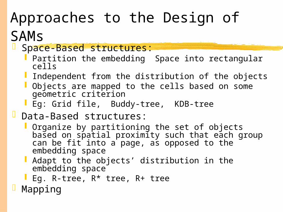
Approaches to the Design of SAMs Space-Based structures:

Partition the embedding Space into rectangular cells

Independent from the distribution of the objects Objects are mapped to the cells based on some

geometric criterion Eg: Grid file, Buddy-tree, KDB-tree

Data-Based structures: Organize by partitioning the set of objects based

on spatial proximity such that each group can be fit into a page, as opposed to the embedding space

Adapt to the objects’ distribution in the embedding space

Eg. R-tree, R* tree, R+ treeMapping

       

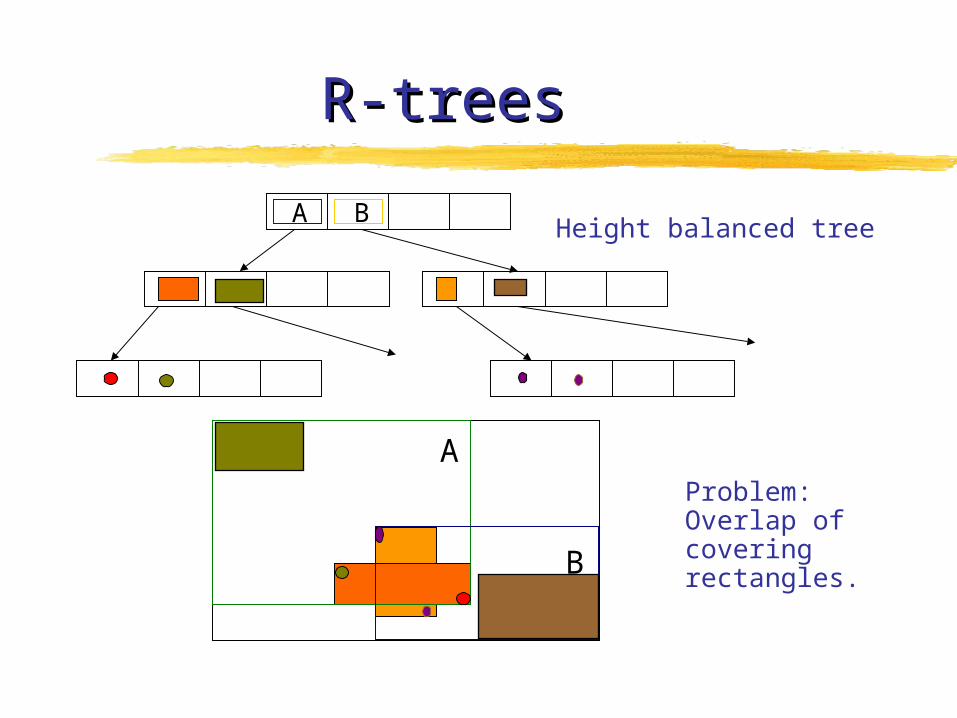
The R-treeA leaf entry is a pair (mbr, oid)A non-leaf node contains an array of node entries The number of entries is between m (fill-factor) and MFor each entry (mbr, nodeid) in a non-leaf node N, mbr is

the directory rectangle of a child node of N, whose page address is nodeid

All leaves are at the same level An object appears in one, and only one of the tree leaves

       

A

B

A B

R-treesR-trees

Height balanced tree

Problem: Overlap of covering rectangles.

Insertion in the R-TreeAlgorithm ChooseSubtreeCS1 [Initialize] Set N to be the root nodeCS2 [Leaf check]

If N is a leaf,return N

else[Choose subtree]Choose the entry in N whose rectangle needs least area

enlargement to include the new data. Resolve ties by choosing the entry with the rectangle of smallest area

endCS3 [Descend until a leaf is reached]

Set N to be the childnode pointed to by the childpointer of the chosen entry. Repeat from CS2

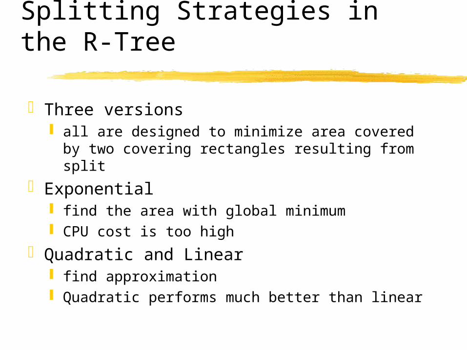
Splitting Strategies in the R-Tree

Three versions all are designed to minimize area covered by

two covering rectangles resulting from split

Exponential find the area with global minimum CPU cost is too high

Quadratic and Linear find approximation Quadratic performs much better than linear

Splitting Strategies in the R-Tree

Algorithm QuadraticSplitAlgorithm QuadraticSplit[Divide a set of M+1 index entries into two groups]QS1 [Pick first entry for each group ]

Invoke PickSeeds to choose two entries, each be first entry of each group

QS2 [Check if done]Repeat

DistributeEntryuntilall entries are distributed or one of the two groups has

Mm+1 entries (so that the other group has m entries)

QS3 [Select entry to assign ]If entries remain, assign them to the other group so that

it has the minimum number m required

Splitting in the R-Tree

Algorithm PickSeedsAlgorithm PickSeeds[Choose two entries to be the first entries of the groups]PS1 [Calculate inefficiency of grouping entries

together]For each pair of entries E1 and E2, compose a rectangle R including E1 rectangle and E2 rectangle

Calculate d = area(R) - area(E1 rectangle) - area(E2 rectangle)

PS2 [Choose the most wasteful pair ]Choose the pair with the largest d

[the seeds will tend to be small, if the rectangles are of very different size (and) or the overlap between them is high]

Splitting in the R-TreeAlgorithm DistributeEntryAlgorithm DistributeEntry[Assign the remaining entries by the criterion of minimum area]DE1 Invoke PickNext to choose the next entry to be assignedDE2 Add It to the group whose covering rectangle will have to

be enlarged least to accommodate It. Resolve ties by adding the entry to the group with the smallest area, then to the one with the fewer entries, then to either

Algorithm PickNextAlgorithm PickNext[chooses the entry with best area-goodness-value in every situation]

DE1 For each entry E not yet in a group, calculate d1 = the area increase required in the covering rectangle of Group 1 to

include E Rectangle. Calculate d2 analogously for Group 2

DE2 Choose the entry with the maximum difference between d1 and d2

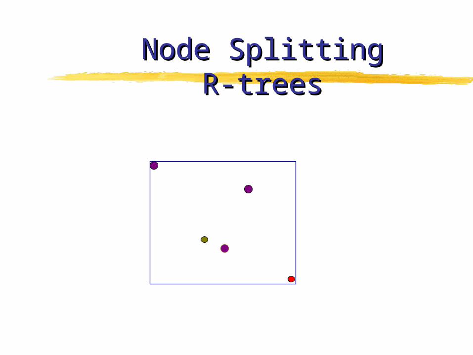
Node Splitting R-treesNode Splitting R-trees

Node Splitting R-treesNode Splitting R-trees

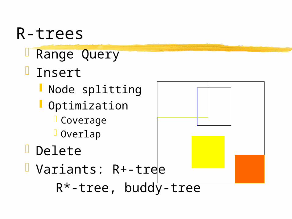
R-treesRange QueryInsert

Node splitting Optimization

CoverageOverlap

DeleteVariants: R+-tree R*-tree, buddy-tree

The R*-Tree

A variant of R-TreeSeveral improvements to the insertion

algorithmAim at optimizing

Node overlapping Area covered by a node Perimeter of a node’s directory rectangle

Given a fixed area, the shape that minimizes the rectangles perimeter is the square

Two variants that bring the most significant improvement

Split AlgorithmForced Reinsertion Strategy

The R+ TreeThe directory rectangles at a given level do not

overlapFor a point query, a single path is followed from the

root to a leaf; for a region query, subtrees whose covering mbr intersecting the query region is traversed

The I/O complexity is bounded by the depth of the tree

Dead space problem

3 - Index Tuning 68

Index Tuning

Index issues Indexes may be better or worse than

scans Multi-table joins that run on for hours,

because the wrong indexes are defined Concurrency control bottlenecks Indexes that are maintained and never

used

Information about indexes...

Application codesV$SQLAREA -- look for the one with

high # of executionsINDEX_STATS: meta information about

indexesHASH_AREA_SIZEHASH_MULTIBLOCK_IO_COUNT…home work

Clustered / Non clustered index

Clustered index (primary index) A clustered index on

attribute X co-locates records whose X values are near to one another.

Non-clustered index (secondary index) A non clustered index

does not constrain table organization.

There might be several non-clustered indexes per table.

Records Records

3 - Index Tuning 71

Dense / Sparse Index

Sparse index Pointers are associated

to pages

Dense index Pointers are associated

to records Non clustered indexes

are dense

P1 PiP2 record

recordrecord

3 - Index Tuning 72

Index Implementations in some major DBMS

SQL Server B+-Tree data structure Clustered indexes are

sparse Indexes maintained as

updates/insertions/deletes are performed

DB2 B+-Tree data structure,

spatial extender for R-tree Clustered indexes are

dense Explicit command for

index reorganization

Oracle B+-tree, hash, bitmap,

spatial extender for R-Tree

clustered index Index organized table

(unique/clustered) Clusters used when

creating tables.

TimesTen (Main-memory DBMS) T-tree

3 - Index Tuning 73

Types of Queries

Point Query

SELECT balanceFROM accountsWHERE number = 1023;

Multipoint Query

SELECT balanceFROM accountsWHERE branchnum = 100;

Range Query

SELECT numberFROM accountsWHERE balance > 10000 and balance <= 20000;

Prefix Match Query

SELECT *FROM employeesWHERE name = ‘J*’ ;

3 - Index Tuning 74

More Types of Queries

Extremal Query

SELECT *FROM accountsWHERE balance = max(select balance from accounts)

Ordering Query

SELECT *FROM accountsORDER BY balance;

Grouping Query

SELECT branchnum, avg(balance)FROM accountsGROUP BY branchnum;

Join Query

SELECT distinct branch.adresseFROM accounts, branchWHERE accounts.branchnum = branch.numberand accounts.balance > 10000;

Index Tuning -- data

Settings:employees(ssnum, name, lat, long, hundreds1,

hundreds2);

clustered index c on employees(hundreds1) with fillfactor = 100;

nonclustered index nc on employees (hundreds2);

index nc3 on employees (ssnum, name, hundreds2);

index nc4 on employees (lat, ssnum, name); 1000000 rows ; Cold buffer Dual Xeon (550MHz,512Kb), 1Gb RAM, Internal RAID controller from

Adaptec (80Mb), 4x18Gb drives (10000RPM), Windows 2000.

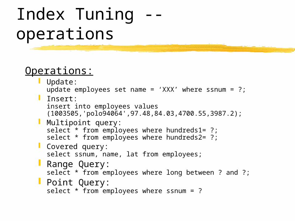
Index Tuning -- operations

Operations: Update:

update employees set name = ‘XXX’ where ssnum = ?; Insert:

insert into employees values (1003505,'polo94064',97.48,84.03,4700.55,3987.2);

Multipoint query: select * from employees where hundreds1= ?; select * from employees where hundreds2= ?;

Covered query: select ssnum, name, lat from employees;

Range Query: select * from employees where long between ? and ?;

Point Query: select * from employees where ssnum = ?

3 - Index Tuning 77

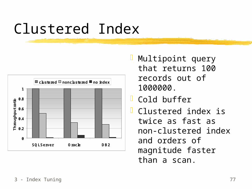
Clustered Index

Multipoint query that returns 100 records out of 1000000.

Cold bufferClustered index is

twice as fast as non-clustered index and orders of magnitude faster than a scan.

0

0.2

0.4

0.6

0.8

1

SQLServer Oracle DB2

Th

rou

gh

pu

t ra

tio

clustered nonclustered no index

Positive Points of Clustering indexes

If the index is sparse, it has less points --less I/Os

Good for multipoint queries eg. Looking up names in telephone dir.

Good for equijoin. Why?Good for range, prefix match, and

ordering queries

3 - Index Tuning 79

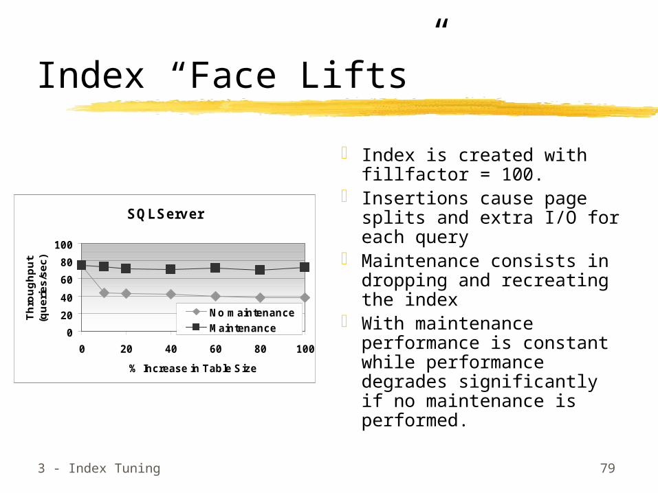
Index “Face Lifts”

Index is created with fillfactor = 100.

Insertions cause page splits and extra I/O for each query

Maintenance consists in dropping and recreating the index

With maintenance performance is constant while performance degrades significantly if no maintenance is performed.

SQLServer

0

20

40

60

80

100

0 20 40 60 80 100

% Increase in Table Size

Th

rou

gh

pu

t (q

ue

rie

s/s

ec

)

No maintenance

Maintenance

3 - Index Tuning 80

Index Maintenance

In Oracle, clustered index are approximated by an index defined on a clustered table

No automatic physical reorganization

Index defined with pctfree = 0

Overflow pages cause performance degradation

Oracle

0

5

10

15

20

0 20 40 60 80 100

% Increase in Table Size

Th

rou

gh

pu

t (q

uer

ies/

sec)

Nomaintenance

3 - Index Tuning 81

Covering Index - defined

Select name from employee where department = “marketing”

Good covering index would be on (department, name)

Index on (name, department) less useful.

Index on department alone moderately useful.

3 - Index Tuning 82

Covering Index - impact

Covering index performs better than clustering index when first attributes of index are in the where clause and last attributes in the select.

When attributes are not in order then performance is much worse.

0

10

20

30

40

50

60

70

SQLSe rv e r

Th

rou

gh

pu

t (q

uer

ies/

sec)

cov e ring

cov e ring - notorde re d

non cluste ring

cluste ring

Positive/negative points of non-clustering indexes

Eliminate the need to access the underlying table eg. Index on (A, B, C) Select B,C From R Where A=5.

Good if each query retrieves significantly fewer records than there are pages in DB

May not be good for multipoint queries

Examples:

Table T has 50-bytes records and attribute A has 20 different values which are uniformly distributed. Page size=4K. Is a nonclustering index on A any good?

Now the record size is 2Kbytes.

3 - Index Tuning 85

Scan Can Sometimes Win

IBM DB2 v7.1 on Windows 2000

Range Query If a query retrieves 10%

of the records or more, scanning is often better than using a non-clustering non-covering index. Crossover > 10% when records are large or table is fragmented on disk – scan cost increases.

0 5 10 15 20 25

% of se le cte d re cords

Th

rou

gh

pu

t (q

ue

rie

s/s

ec

)

scan

non clustering

3 - Index Tuning 86

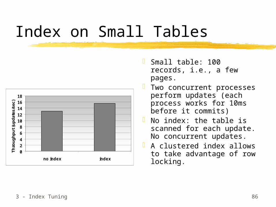
Index on Small Tables

Small table: 100 records, i.e., a few pages.

Two concurrent processes perform updates (each process works for 10ms before it commits)

No index: the table is scanned for each update. No concurrent updates.

A clustered index allows to take advantage of row locking.

0

2

4

6

8

10

12

14

16

18

no index index

Th

rou

gh

pu

t (u

pd

ates

/sec

)

Bitmap vs. Hash vs. B+-Tree

Settings:employees(ssnum, name, lat, long, hundreds1,

hundreds2);create cluster c_hundreds (hundreds2 number(8)) PCTFREE 0;create cluster c_ssnum(ssnum integer) PCTFREE 0 size 60;

create cluster c_hundreds(hundreds2 number(8)) PCTFREE 0 HASHKEYS 1000 size 600;

create cluster c_ssnum(ssnum integer) PCTFREE 0 HASHKEYS 1000000 SIZE 60;

create bitmap index b on employees (hundreds2);create bitmap index b2 on employees (ssnum);

1000000 rows ; Cold buffer Dual Xeon (550MHz,512Kb), 1Gb RAM, Internal RAID controller from Adaptec

(80Mb), 4x18Gb drives (10000RPM), Windows 2000.

3 - Index Tuning 88

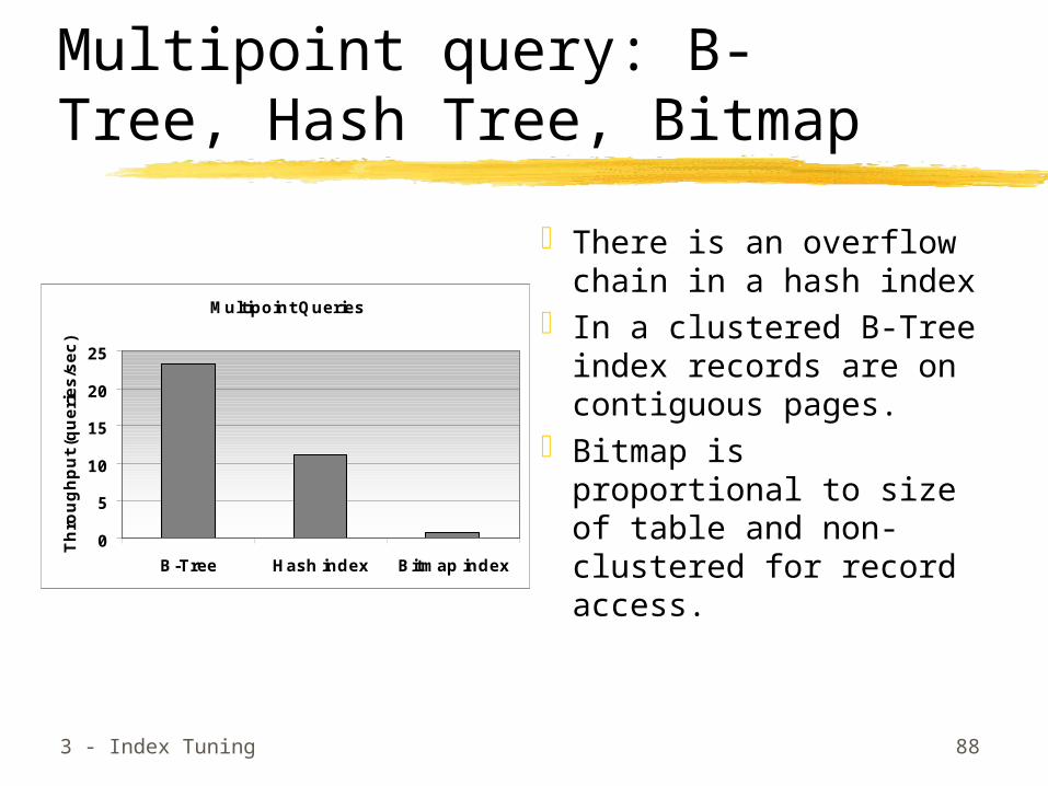
Multipoint query: B-Tree, Hash Tree, Bitmap

There is an overflow chain in a hash index

In a clustered B-Tree index records are on contiguous pages.

Bitmap is proportional to size of table and non-clustered for record access.

Multipoint Queries

0

5

10

15

20

25

B-Tree Hash index Bitmap index

Th

rou

gh

pu

t (q

ue

rie

s/s

ec

)

3 - Index Tuning 89

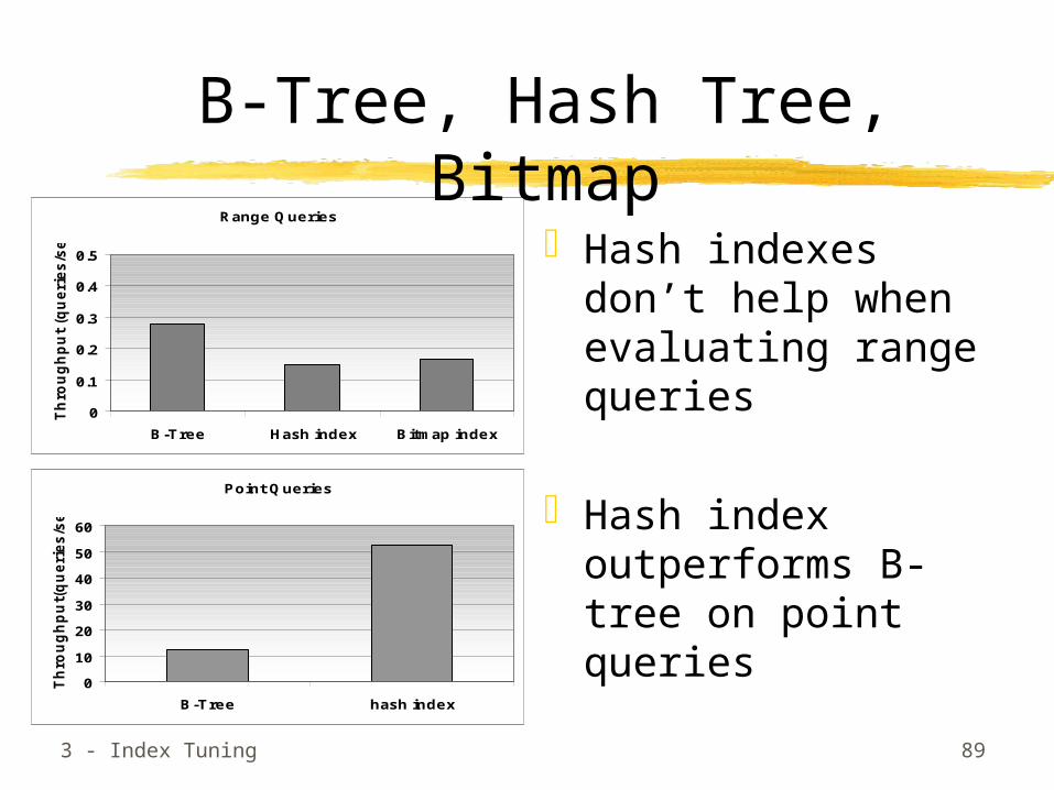
Hash indexes don’t help when evaluating range queries

Hash index outperforms B-tree on point queries

Range Queries

0

0.1

0.2

0.3

0.4

0.5

B-Tree Hash index Bitmap index

Th

rou

gh

pu

t (q

ue

rie

s/s

ec

)

B-Tree, Hash Tree, Bitmap

Point Queries

0

10

20

30

40

50

60

B-Tree hash index

Th

rou

gh

pu

t(q

ue

rie

s/s

ec

)

Summary

Primary means to reduce search costs (I/O and CPU)

Properties: robust, concurrent, scalable, efficient

Most supported indexes: Hash, B+-trees, bitmap index, and R-trees

Tuning: Usage, Maintenance, Drop/Rebuild, index locking in buffer...