cs379h undergraduate thesis -...

CS379H Undergraduate ThesisPolyphonic Guitar Transcription by Bayesian Methods

Mark KedzierskiUniversity of Texas at Austin, Department of Computer Sciences2005

Abstract

I present a method of transcribing Polyphonic guitar music using probabilistic modeling. The generative model an expanded version of the one found in (Cemgil, 2004). The piano roll, or score, of the given audio waveform is inferred using MAP (Maximum A Posteriori) trajectory estimation via a Switching Kalman Filter. Because exact inference is generally intractable on Switching Kalman Filters, pruning and approximation methods are used. Integral approximation is achieved by Kalman filtering recursions.

To make the model useful, and to expand on previous work, (Kedzierski, 2004), my generative model applies many restrictions to limit the size of the state space. The performance is restricted to a single guitar which can play at most 6 simultaneous notes. The Prior probability over the notes is novel and includes knowledge of tonality, tempo, composition structure, as well as the physical distances between notes on the neck of the guitar.

The goal of this paper is to step closer to a real-time polyphonic MIDI sequencer Virtual Studio Technology plug-in. This could be used for composition, performance, and the driving of virtual musicians/instruments.

2 CS379 Honors Thesis - Mark Kedzierski

Table of ContentsI. IntroductionII. Related WorksIII. Physical Properties of Sound WavesIV. Music Theory PrimerV. MIDI PrimerVI. State Space Models and Linear Dynamical SystemsVII. Bayes NetworksVIII. Damped Oscillator ExampleIX. Multinormal DistributionX. Kalman FilterXI. Switching Kalman Filter model for monophonic melodiesXII. Polyphonic Chord TranscriptionXIII. Extending to the PriorXIV. Instrument Parameter LearningXV. Future WorkXVI. Bibliography

CS379 Honors Thesis - Mark Kedzierski 3

IntroductionIn this report I will outline a solution to the problem of polyphonic music transcription based on Bayesian

inference. Specifically, transcribing a digital recording of a single guitar player. The applications of this capability include music education, composition, and recording.

Transcription is strongly related to the measurement of pitch in an audio signal; a problem which has been long investigated due to it's many potential appications. It is a difficult one, however, because pitch is a subjective attribute which cannot directly be measured. Pitch is defined as the characteristic of a sound which places it at a specific loca-tion in the musical scale. The ability to detect it varies among different people. Some are born with “perfect pitch”, which means that they can accurately classify the pitch of a sample sound without any reference. Most people how-ever, can only detect intervals, or the difference in pitch between different sounds. Some suggest that pitch detection might be a learned ability, as different cultures often have different musical scales, each with different intervals. In any case, it is difficult to detect any attribute which is, by definition, subjective. The first approach I took to solving this problem was to determine the fundamental frequency of the audio sample, in blocks (windows), and use it to classify its pitch. While this approach resulted in an effective real-time algorithm to detect the pitch of monophonic digital audio, it is ineffective in polyphonic applications. In this paper I explore a method of transcribing Polyphonic guitar music using probabilistic modeling. First, we define a state space model, based on (Cemgil, 2004), for generating audio signals not unlike those of stringed instru-ments. We then use our generative model to infer the most likely piano roll, i.e. a musical score, which would gener-ate the audio waveform. The piano roll describes the musical performance which caused the digital audio data. This is done by generating waveforms for every possible piano roll and comparing them to the source. The closest waveform would give us the correct piano roll. In practice, (because we can't realistically make all those calculations), we do this in real-time as a Viterbi MAP state trajectory estimation problem using Switching Kalman Filters (Murphy, 1998). This means we propagate the most likely sequence of states which led to the current audio sample. The implementation of my research has been developed in Matlab. The program is capable of learning parame-ters from sampled audio data as well as Viterbi MAP trajectory estimation for polyphonic music. I planned to imple-ment the code as a VST plug-in, but didn't have time. VST would allow the product to be used in conjunction with a variety of professional audio software. The remainder of this document consists of several sections. I have attempted to order the document in such a way that all necessary background theory is presented before its application. However, some background in probability/statistics is assumed. In the first section I mention related works. Next I describe those physical properties of sound waves which are relevant to music. Third, I provide a primer in the music theory necessary to understanding the implementation. Fourth, I explain the MIDI standard and how it enables digital instruments to communicate. Finally, I outline the solution of a simplified problem, as well as the algorithms/models utilized in the final implementa-tion. To close the document I summarize results from actual experiments and propose future enhancements the system.


Related WorksThis is work is largely based on a Ph.D. thesis by Ali Cemgil (Cemgil, 2004). He outlined a generative Switch-

ing Kalman Filter model for plucked string audio waveforms as well as Bayesian inference algorithms to implement polyphonic music transcription. The model is defined, in general, as a Dynamic Bayesian Network (DBN) such as those defined in (Murphy, 2004). The solution works very effectively for monophonic melodies and usually works for polyphonic. The errors in polyphonic transcription case arise from the hill-climing algorithm getting stuck on local maxima.

In this paper I propose to increase performance of inference by expanding the prior distribution over piano rolls with knowledge of tonality and by applying various limitations to Cemgil's generative model. I also describe my implementation of the inference and learning algorithms using Matlab.


Physical Properties of Sound WavesIn this section I discuss the physical nature of sound as relevant in the discussion of musical tones and/or

melodies. We define pitch as any the attribute of sound which defines its placement on the musical scale. We define a tone as any sound which is associated with a pitch. First I offer a concise explanation by Brian C.J. Moore: “Sound originates from the motion or vibration of an object. This motion is impressed upon the surrounding medium (usually air) as a pattern of changes in pressure. What actually happens is that the atmospheric particles, or molecules, are squeezed closer together than normal (called condensation) and then pulled farther apart than normal (called rarefac-tion).” (Moore, 1999) We obtain a graphical representation of a sound be plotting the amplitude of pressure variation over time. We call this plot a waveform. I provide an example below. Note because waveforms are a plot against time, they are said to exist in the time-domain.

Figure 1

This waveform is known as a pure-tone; plotted as pressure variation over time. Remember that a tone is defined as any sound which can be classified as having a pitch. A gunshot is not a tone. A pure tone is named for its very “clean” musical sound, very much similar to that of a tuning fork. A pure tone’s waveform is simply a sine wave, whose frequency determines where the note lies on the musical scale. For example, the commonly used A-440 tuning fork produces a wave very similar to a 440 Hz sine wave. We will discuss this in

greater detail in the next section.

While pure tones are important in defining pitch and useful in theoretical discussion, we do not encounter them in nature. Instead, we see complex-tones. Like pure-tones, all complex tones are assigned a unique pitch value. But instead of consisting of a single sine wave at a given frequency, they contain several superimposed sine waves, all located at harmonics. More accurately, a complex tone consists of a fundamental frequency and several overtones.

We define the ith harmonic of a given frequency as the ith integral multiple of said frequency. For example, the 0th, 1st, and 2nd harmonics of a 440Hz tone would exist at 440Hz, 880Hz, and 1320Hz, respectively. We define the fundamental frequency of a complex tone to be the 0th harmonic. We similarly define any tones which occur at subsequent harmonics as overtones of that fundamental frequency. The next figure depicts sine waves of frequencies at 3rd, 4th, and 5th harmonics combined to form a complex tone.


Figure 2

Complex tone, containing 3 overtones.

The sound generated from a plucked guitar string is an example of a complex tone. The waveform is shown below. Note how it resembles a damped sin wave, with the amplitude decreasing over time.

Figure 3

Sampled waveform of a plucked guitar string. This is an example of a complex tone.


Music Theory PrimerTo begin our primer on music theory, we define a note as any named tone. The ordered collection of all

possible notes is known as the musical scale. We define an interval as the spatial distance, on the musical scale, between successive notes. Commonly occurring intervals are given names. The smallest interval is the ½-step (or semitone), which is used to represent the distance between two adjacent notes on the scale. The Whole-step is the equivalent of two ½-steps. Some other commonly occurring intervals are the Fifth, Major Third and Minor Third. We can now define a melody as a series of notes played at varying intervals.

The musical scale is logically divided into groups of twelve notes known as octaves. Every octave consists of twelve semitones which are labeled in the following manner: C, C#/Db, D, D#/Eb, E, F, F#/Gb, G, G#/Ab, A, A#/Bb, B. We use this scheme because each of these labels represents a unique “sound”, only twelve of which exists. This means that a C note sounds the “same” as a C note in any other octave. Each octave in the musical scale is labeled by an index, starting at 0. In turn, every note on the musical scale can be uniquely identified by a note label and octave index. Examples are: C0, Db5, and G2. Middle C is represented as C4. So, if we know the pitch of a tone, we know where it belongs on the musical scale. But since real instruments don’t make pure tones, we need a way to assign pitch. “Since pitch is a subjective attribute, it cannot be measured directly. Assigning a pitch value to a sound is generally understood to mean specifying the frequency of a pure tone having the same subjective pitch as a sound.” (Moore, 1999). We define the relative frequency (ç) of any note ç as the frequency of said pure tone. For example, (C4) = 261.4Hz. Next we discuss how the musical scale maps to the human audible frequency range.

The human audible frequency range is approximately 20-20,000Hz. However, we are not concerned with anything above 5Khz, as we are unable to discern the pitch of frequencies in the that range. (Moore, 1999) The range of 0-5kHz is partitioned into eight octaves, each beginning at C, where (C0)=16.4Hz, (C1)=32.7Hz, (C8)=4186Hz. It may be clear now why C4 is known as middle C. You may notice that (C1) = 2(C0). This leads us to the real defini-tion of the octave as the interval between two tones when their frequencies are in a ratio 2:1 (Moore, 1997) We can deduce from this that the eight octaves are not the same size, instead they increase exponentially. Every interval, in fact, is actually a relationship between two tones. The following table depicts common intervals and their associated ratios:

Table 1

Interval Ratio ½ step 1:1.05946 Fifth 3:2 Maj Third 5:4 Min Third 6:5

Description of common intervals


MIDI PrimerThe Musical Instrument Device Interface is widely used by musicians to communicate between digital musical

instruments. It is a standard which has been agreed upon by major manufacturers in the industry. It connects not only musical instruments, but all devices such as recorders and lighting systems.

The communication in a MIDI system is done by sending and receiving messages. Examples of some mes-sages related to melody composition are Note-On, Note-Off, Tempo Change, Key-Signature Change, and Time-Signa-ture change. The meanings behind these events are self-explanatory. Each message contains variables specific to the message. For example, a Note-On event would contain information about which note should be played, and the volume at which it should be played. Each note is assigned a specific index. These indices are standard and are listed in Appendix A. The Key-Signature message would contain the new desired key signature.

In practice a synthesizer driver would create and dispatch a series of MIDI messages to a synthesizer. The synthesizer would then playback the desired notes using pre-recorded instrument audio samples.


State Space Models and Linear Dynamical SystemsBayesian inference problems involve making estimates of the current state of a graphical state-space system

model, given uncertain or incomplete data. This consists of defining a graphical system model and then performing inference algorithms on the model.

à Dynamical State-Space Models

A state-space system model consists of a set of equations which synthesize the output of some physical system. Though not always the case, in this paper I limit discussion to systems which operate/evolve as a function of time (a.k.a. Dynamical Systems ).

The system is defined, among other things, by the set of possible 'situations', or states, that it can be in at any particular time. The state variable, st, represents the current state of the system at each time t, {t: 0§t§T}. This can be represented as a single variable, or a vector; with continuous or discrete values. The length of a state vector, » st », is labeled as N (N=1 in single variable case). The sequence state variables, s0:T , are responsible for generating the output of the system. The actual information stored in the state variable depends on the system being described. In addition to the state variable, all we need to define a system is a state transition function, ,

(1)st = Hst-1L,» st » = N

which describes how the state of the system changes over time. As time progresses through each time-step, the state variable will change to reflect the current time-slice. In practice, the definition of can depend on a vector of some other constant parameters, q.

(2)st = Hst-1, qL,

Notice that this is a recursive definition. We can then run a simulation of our system over T time-slices, (i.e. calculate the progression of states, s0:T ), by specifying the base case, s0, and parameter vector q.


ü System Observations

In cases where the observed output of a physical system is digitally sampled, the output does not correspondexactly to the set of state vectors. Instead, it is a function of the current state. In this case we add another 'layer' ofvariables, y1:T , to represent the observations. The length of an observation vector, » yt », is given as M (M=1 in singlevariable case). Where the value of each observation is given by the observation function, .

(3)yt = Hst, qL» yt » = M

In this case we don't need an initial value, as the definition is not recursive. In summary:

Table 2

s0 = p,st = Hst-1, qL,

yt = Hst, qL» st » = N» yt » = M

The top layer of nodes, s1:T , represent the state vector. The bottom layer, y1:T , represents the observed data.

à Linear Dynamical Systems, (LDS's)

If we only consider models with linear transition functions we are dealing with Linear Dynamical Systems (LDS's). This linearity enables us to define the transition and observation functions using square transformation matrices A and C, respectively. The new equations are:

(4)st = A st-1

yt = C st, where

where A is a NäN matrix and C is a 1äM matrix. An example of a such a system is a damped sinusoid with a constant angular frequency w. The definition of the state-space model follows in the damped oscillator example.


ü Adding some 'randomness'

The above definitions, given s0 and q, are enough to describe a fully deterministic model. This means that we can tell with certainty what values of s0:T , y0:T will be: we can simply plug in the initial variables and calculate each time-slice. While a good start, this is not a realistic model of a sound wave. We need to model both noise in the state transitions, to account for minute frequency/damping variations, as well as observation noise. The latter models the noise introduced by digitizing the wave with recording hardware. This will create a more realistic, i.e. 'noisy', sound wave. We do this adding noise terms to both the state and observation vectors:

(5)st = A st-1 +

(6)yt = C st +

ü Modelling process noise

The process noise is defined as white gaussian. A noise is white when it is not correlated through time; its value at any time t is not dependant to any other time period. It's labeled as gaussian because it is drawn from a normal (gaussian) distribution. It particular, a zero-mean gaussian with diagonal covariance matrix Q:

(7)~ J@0 0D, JQ11 00 Q22

NN

where (m,S) represents a multivariate gaussian distribution with mean m and covariance matrix S. x ~ (m,S) means that x is a random variable, the value of which is drawn from the distribution. We can see how the diagonal terms of Q add noise the state vector. We can simplify (10) to get:

(8)st = A st-1 + H0, QL

st ~ HA st-1, QL

ü Modelling observation noise

The definition of the observation noise is identical to the process noise except for the dimensionality. We define a observation noise covariance matrix R and write:

(9)yt = C st + H0, RL

yt ~ HC st, RL


ü Modelling state transitions with conditional probability distributions

The noise terms now render the system model indeterministic. This means that we are no longer predict, with full certainty, the values of future state variables. Both the transition and observation functions are continuous vari-ables represented as conditional probability distributions.

Table 3

q = 8A, C, Q, R, p<s0 = p

st ~ pHst » st-1L ª HA st-1, QLyt ~ pHyt » stL ª HC st, RL

Where q represents the given parameter constants. p is also given as the initial state.

The term pHyt » stL is known as the likelihood of the observation. It will be explained in later sections.

ü Hidden / Observed variables

It is important to label the variables in our model as hidden or observed. The observation terms, y1:T , are obviously observed. The state vectors are hidden terms. They are considered hidden because we can't directly measure them in any way. We can only derive them past state variables. This is a big problem when we don't have the initial state vector, s0, from which to calculate s1..., then s2; all we have are noisy state observations, y1:T . How can we find the values of these hidden state variables? The answer is to find the joint distribution pHs1:T , y1:T L by utilizing the conditional independence structure of the graphical model. This is known as filtering. It is useful to first review Bayes Belief Networks.


Bayes Networks

ü Definition

Probabilistic graphical models are directed graphs which represent joint probability distributions (Murphy, 2004). Arrows between nodes represent conditional probabilities; while lack of arrows represent conditional indepen-dance. More specifically, the value of each node, X, is a probabilty distribution conditioned on it's parent nodes, Pa( X ).

(10)pHX » PaHX LL = ¤i=1N pHxi » PaHxiLL

ü Conditional Independence, Local Markov Property

One real benefit of using a Bayes nets is the conditional independence assumption, i.e. that each node X is conditionally independant of its non-descendants given its parents, Pa(X). This is known as the Local Markov Prop-erty.

Figure 4

Local Markov Properties of Bayes nets. (a) A node X is conditionally independant of its nondescendants (e.g. Z1 j , ..., ZnjL given its parents U1, ..., Um. (b) A node X is conditionally indepenendant of all other nodes in the

network given its Markov blanket (shaded). From [RN02].

This representation allows calculation the joint probability distribution of all the nodes by using the junction treealgorithm (i.e. Filtering) (Murphy, 2004).


ü Filtering

The most common problem in Bayesian statistics is propagating a joint state distribution. This done by running 'forward' and 'backward' passes across the graph. For example, consider the graphical model in the next figure, (Mur-phy, 2004)

Figure 5

(Murphy, 2004)

The joint distribution is given by:

(11)P(A,B,C,D, F,G) = P(A)P(B|A)P(C|A)P(D|B,A)P(F|B,C)P(G|F)

The conditional independance assumptions lead to the following factorization of the joint distribution.

We can marginilize one variable at a time, working from right to left:

where lGØFHFL = ⁄G PHG » FL.The forward pass starts from the root node and propagates the forward 'message', p, by repeatadly calculating

the conditional distributions for all child nodes. The backward 'message', l, starts from the leaves and propagates the


state distribution back to the root. Each step consists of marginalizing and conditioning. This is shown graphically inthe next figure.

Figure 6


ü Estimating values of hidden variables, a.k.a. filtering

The answer is to infer the values of the hidden variables, s0:T , conditioned on noisy observations. This is the most common problem in Bayesian statistics and is known as filtering. Think of filtering out the noise and returning the pure source of the observations.

Because the values of the hidden variables are unobserved and indeterministic, we can only make estimates, s1:T . The hat symbol, ^, indicates an estimated or predicted value.

Because we are making estimates of the hidden variables (a.k.a. state estimate, or belief state), we also associ-ate a degree of belief with our estimate. This is the essence of Bayesian probability: we use probabilities to represent the certainty in an estimate. More specifically, the belief state at time t is a probability density (i.e. normalized distribu-tion) over all possible states at time t given the observations, i.e. pHs1:T » y1:T L. This is known as the posterior distribu-tion, or filtering density. It can be calculated using an the prior state estimate, the likelihood of the evidence given the estimate, and Bayes' Theorem:

(13)pHs1:T » y1:T L ªpHy1:T »s1:T L pHs1:T LÅÅÅÅÅÅÅÅÅÅÅÅÅÅÅÅÅÅÅÅÅÅÅÅÅÅÅÅÅÅÅÅÅÅÅÅÅpHy1:T L

Same equation with labeled terms is:

(14)Posterior ª likelihood ä priorÅÅÅÅÅÅÅÅÅÅÅÅÅÅÅÅÅÅÅÅÅÅÅÅÅÅÅÅÅÅÅÅÅÅÅevidence

The prior probability is propagated from the initial state estimate, p ª pHs0),

(15)pHs1:T L ª p pHs0 » s1L pHs1 » s2L pHs2 » s3L ... pHsT-1 » sT L

The likelihood term is defined in the generative model.

The normalization factor, or evidence, is the sum of the marginal likelihoods of the data for all states st:

(16)pHy1:T L ª Ÿs1:TpHy1:T » s1:T L pHs1:T L

In general, ⁄ is used to marginalize over discrete variables, Ÿ is used to marginalize continuous variables. For LinearDynamical Systems, the marginilization can be done using the Kalman Filter equations.


Damped Oscillator ExampleThe generation of a digitally sampled damped sinusoidal of frequency w can be stated as a linear dynamical

system given by (Cemgil, 2004). We assume that our observations of the system are digital samples taken at a constant rate Fs.

ü Observations - y1:T

At each time slice the observation represents a single audio sample. The value of yt represents the amplitude of the wave at time t. It has only a single component, so M=1.

ü State Vector - s1:T

The waves can be generated by a two-dimensional oscillator vector, st, which rotates around the origin with an angular frequency w. The length of vector st corresponds to the initial amplitude of the sinusoidal and decreases over time at rate constant r. This is called the damping coefficient. Because the variables w and r stay constant for a given model, they are parameters,

(17)q = {w, r}

System parameters

The observations are generated by projecting the 2-dimensional state vectors onto a 1-dimensional plane (over time). This is depicted in the figure below (Cemgil, 2004).

Figure 8

A damped oscillator in state space form. Left: At each time step, the state vectorst rotates by w and its length becomes shorter. Right: The actual waveform is a one dimensional projection from the two

dimensional state vector.


ü Initial state estimate - p

The initial state estimate, p ª pHs0L is drawn from a zero-mean gaussian with covariance matrix S.

(18)p ~ H0, SLThe diagonal sum of S, Tr(S), is proportional to the initial amplitude of sound wave. The covariance structure defineshow the 'energy' is distributed along the harmonics (Cemgil, 2004). It is initially estimated with a strong 1st and 2ndharmonics. The later overtones have increasingly less energy. This pattern can be shown by a Fourier transform of theaudio signal.

Figure 9

Top: Audio signal of electric bass. Originally at 22 kHz, down-sampled by factor D=20. Middle: Frequency Spectrum (DFT) of audio signal Bottom: Diagonal entries of S for H=7 correspond to overtone amplitudes


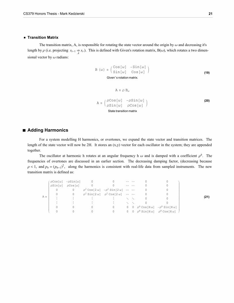
ü Transition Matrix

The transition matrix, A, is responsible for rotating the state vector around the origin by w and decreasing it's length by r (i.e. projecting st-1 fl

A st.). This is defined with Given's rotation matrix, B(w), which rotates a two dimen-

sional vector by w radians:

(19)B HωL ≡ J Cos@ωD −Sin@ωD

Sin@ωD Cos@ωD N

Given' s rotation matrix.

(20)

A ≡ ρ Bω

A ≡ J ρCos@ωD −ρSin@ωDρSin@ωD ρCos@ωD N

State transition matrix

à Adding Harmonics

For a system modelling H harmonics, or overtones, we expand the state vector and transition matrices. Thelength of the state vector will now be 2H. It stores an (x,y) vector for each oscillator in the system; they are appendedtogether.

The oscillator at harmonic h rotates at an angular frequency h w and is damped with a coefficient rh. Thefrequencies of overtones are discussed in an earlier section. The decreasing damping factor, (decreasing becauser < 1, and ph = Hph-1L2, along the harmonics is consistent with real-life data from sampled instruments. The newtransition matrix is defined as:

(21)A ≡

i

k

jjjjjjjjjjjjjjjjjjjjjjjjjjjjjjjjjjjjj

ρCos@ωD −ρSin@ωD 0 0 ∫ ∫ 0 0ρSin@ωD ρCos@ωD 0 0 ∫ ∫ 0 0

0 0 ρ2 Cos@2 ωD −ρ2 Sin@2 ωD ∫ ∫ 0 00 0 ρ2 Sin@2 ωD ρ2 Cos@2 ωD ∫ ∫ 0 0ª ª ª ª ∏ ∏ 0 0ª ª ª ª ∏ ∏ 0 00 0 0 0 0 0 ρH Cos@H ωD −ρH Sin@H ωD0 0 0 0 0 0 ρH Sin@H ωD ρH Cos@H ωD

y

{

zzzzzzzzzzzzzzzzzzzzzzzzzzzzzzzzzzzzz


ü Observation Matrix

The observations are simply projections of the state vector. We define the observation matrix as 1ä2H dimen-sional projection matrix:

(22)C = [0 1 .... 0 1]Observation matrix

ü Summary of generative model

Table 4

q = 8w, r, H , Q, R, p<s0 = p

st ~ pHst » st-1L ª HA st-1, QL yt ~ pHyt » stL ª HC st, RL

Where q represents the given parameter constants, as in (6). p is also given as the initial state.

The term pHyt » stL is known as the likelihood of the observation. It will be explained in later sections.


Multinormal Distribution

ü Definition

Let X œ d represent a normally distributed random vector. Then we write,

(23)X ª @x1, x2, x3, ... xi, ... xdDX ~ (m,S) m ª @m1, m2, m3, ... mi, ... mdD

m represents the mean value and S represents the covariance matrix. Each index (i,j) in the covariance matrix holds thevalue covHxi, x jL.

ü Probability Density Function

The probability density function (PDF) of a multi-variate gaussian (multinormal) distribution is given by:

(24)p(x) = (m,S)

= » 2 pS »- 1ÅÅÅÅ2 expH- 1ÅÅÅÅ2 Hx - mL S-1Hx - mLL

ü Mean - mx

The mean of multinormal distribution, X ~ Hmx, SxL, is equivilent to the expected value of X.

(25)mx ª EHX L ª Ÿi pHxiL xi dx

This is also known as the first order moment of p(x).

ü Variance

The variance is the second order central moment of the probability density function (Ahrendt, 2005).

(26)varHX L ª EHHX - mL2L


ü Covariance - Sx

The covariance is also a second order moment,

(27)covHi, jL ª EHHxi - miL Hx j - m jLL

The covariance matrix is an NäN matrix where Si, j holds the value covHxi, x jL.

ü Linear transformations of normally distributed random variables

Let A, B œ c*d and c œ d . Let X ~ Hmx, SxL and Y ~ Hmy, SyL be conditionally independent (Ahrendt, 2005).

(28)Z = AX + BY + c ~ N(AX + BY + c, ASxA + BSxB )

ü Marginilization

Let @x1, x2, ..., xc, xc+1, ..., xND ~ Hmx, SxL. This is a joint probability distribution, pHx1:N L. If we with tofind pHx1:cL, we have to marginilize over variables xc+1:N ,

(29)pHx1, ..., xcL = Ÿ ... Ÿc+1:N pHx1, ... xN L dxc+1 ... xN

Finding the mean and covarance of the marginal distribution is done by extracting the corresponding elements from thejoint distribution (Arhendt, 2005).

(30)pHx1, ..., xcL = pHx1:cL = 1:cHm1:c, S1:cLwhere m1:c = @m1, ..., mcD and

(31)S1:c =

i

k

jjjjjjjjjjjjj

c11 c21 ∫ c11

c12 c22 Ñ ªª Ñ ∏ ª

c1 c ∫ ∫ ccc

y

{

zzzzzzzzzzzzz

ü Conditioning

Let X ~ Hmx, SxL be represented with the following mean and covariance:

(32)m = Jm1

m2N and S = JS11 S12

S21 S22N

The conditional distribution, pHx1 » x2L, is also a normal distribution,

(33)pHx1 » x2L ~ Hm1 + S12 S22-1Hx2 - mxL, S11 - S22

-1 S12T L


Kalman Filter

ü System Model

The Kalman Filter is a set of equations which can be used to propagate the state estimate of a Linear Dynamical System with white gaussian noise. The observations of such a system result from the following equations:

(34)st = A st-1 +

(35)yt = C st +

ü Message Representation

Inference on Kalman Filter Models is equivilent to the junction tree algorithm; but is more complicated due to the continuous random variables. We propagate an estimate represented by the 1st and 2nd order statistical moments of the state distribution (Welch):

(36) pHxk » ykL ~ HE@xkD, E@Hxk - xkL Hxk - xkL DL

ª Hxk, PkLwhere,

(37)xk = E@xkD

Pk = E@Hxk - xkL Hxk - xkL D

ü Filtering Algorithm

From the recursive definitions above we see that posterior distribution is initially estimated and then propagated across time-slices. This is done in a cycle of prediction and correction equations.

Figure 10

The ongoing discrete Kalman filter cycle. The time update projects the current state estimate ahead in time. The measurement update adjusts the projected estimate by an actual measurement at that time. Figure taken

from (Welch, 2001)


Conditioned on the prior distribution from t-1 (or p in case of t=1), a prediction of the next audio sample (a.k.a. a priori estimate) can be calculated from the current belief state using the kalman prediction equations.

ü a Priori state estimate

The a priori estimate is a prediction. Consider it as a initial estimate 'before' observing yt,

(38)dt»t-1 ª Ÿst-1pHst » st-1, y1:t-1L,

The Kalman filter predict equations calculate a priori estimate as a linear transformation of the previous state distribution estimate. See (29):

(39)sk- = A sk-1

(40)Pk- = A Pk-1 A + Q

This projection of the state vector across time slices, st-1 ØA

st, corresponds to marginalization over st-2. This is due to the Local Markov Property (i.e. st is conditionally independent of st-2, given st-1).

In the correct step, we use the observation estimate, yt»t-1, along with observed sample, yt, to calculate the conditional likelihood of the observation.

ü a Posteriori state estimate

The a posteriori estimate is the result of the priori estimate conditioned on yt.

(41)dt»t-1 ª pHyt » stL dt»t-1,

This is calculated by adjusting the priori estimate using our predicted covariance and a weighted estimate error,defined next.


ü Estimate errors

Let xk, xk- œ N , represent the a posteriori and a priori state estimates and time-step k. The estimate errors

are given as (Welch)

(42)ek

- ª xk - xk-, and

ek ª xk - xk.

The a priori estimate covariance is

(43)Pk- = EHek

- ek- L

The a posteriori estimate covariance is

(44)Pk = EHek ek L

ü Kalman Filter Gain

Our goal is to propagate an estimate such that the posterior error covariance is minimized. At each time step,we update our previous estimate using the difference in our predicted measurement, C xk

-, and the actual observedmeasurement, yk . This difference is known as the residual, or the innovation in the measurement.

The minimization is done by substituting equation (22) into the definition for ek, (Welch)

(45)

ek ª xk - Hxk- + KkHyk - C xk

-LLª xk - xk

- - KkHyk - C xk-L

ª ek- - KkHyk - C xk

-Lsubstituting that into equation (18),

(46)Pk = EHHek- - KkHyk - C xk

-LL Hek- - KkHyk - C xk

-LL Lperforming the indicated expectations, taking the derivative of the trace of the result with respect to K, setting thatresult equal to zero, and then solving for K, known as the blending factor: (Welch)

(47)Kk = Pk- C HC Pk

- C + RL-1

ü Correction Equations

The Kalman filter update equations:

(48)Kk = Pk

- C HC Pk- C + RL-1

xk = xk- + KkHyk - C xk

-LPk = HI - Kk CL Pk

-


Switching Kalman Filter Model for Monophonic MelodiesIn this section the model is expanded to model a piano roll representation. The piano roll, or score, is a

sequence indicators which label each time-slice with a state of sound, or mute. We define values sound=1 and mute=2 for simplicity.

ü Transition Matrices

We need to define transition matrices, 8Asound, Amute<, for each state of the oscillator. They are the same as before except for the damping coefficient:

(51)Asound ≡ ρsound B HωLAmute ≡ ρmute B HωL

rsound is slightly less than 1. rmute is much smaller than rsound.

ü Defining the switch variables - r1:T

The variables are referred to as switch variables because, at each time-step, they select which of two transition functions is used to project the next state. The two transition functions represent the sound and mute states:

(52)r1:T ª 8 rt : rt œ 8sound fl mute<, 0 § t § T<For every 2-slice period, there are four possible combinations of rt-1:t. The distribution of the configurations defines the prior on piano rolls. They can be organized as:

(53)pHr1L ª uH8sound, mute<L ª @.5, .5D

(54)

p Hi, jL ª p Hrt = i » rt-1 = jLª 9 pHrt = 1 » rt-1 = 1L pHrt = 1 » rt-1 = 2L

pHrt = 2 » rt-1 = 1L pHrt = 2 » rt-1 = 2L=

ªikjjj1 - 10-7 10-7

10-7 1 - 10-7y{zzz

The initial prior is a uniform distribution. The conditional distribution is a multinomial where it is much more likely for the switch variable to remain the same over time slices. We also define the function, isonsett. It is true if there has been a note onset at the current time slice. A note onset is represented by the mute to sound transition. The updated model is as follows:


à Inference for the Switching Kalman Filter model

ü Viterbi Estimation

Given an audio waveform, our goal is to infer the most likely sequence of piano roll indicators, r1:T* , which

could give rise to the observed audio samples. This is, in general, a Viterbi estimation problem. The value we are seeking is defined as the Maximum A Posteriori trajectory:

(55) r1:T* ª argmax

r1:T

pHr1:T » y1:T L

It represents the most likely sequence of hidden variables to cause an observed output. This is different from the posterior distribution because it is just a point estimate. Calculation is the same as for filtering, except for replacing the summation over rt-2 with the maximization (MAP). It is important to note that, in Viterbi estimation, we propagate a filtering potential, d1:T , as opposed to a filtering density, a1:T . The term potential used to indicate that this value is not normalized. Because we only care about the best piano roll, (i.e. configuration rt:T with highest likelihood), we can save calculations by using a point estimate.

(56)pHr1:T » y1:T L ∂ ŸstpHy1:t » st, r1:tL pHs1:t » r1:tL pHr1:tL

filtering potential


ü Prediction

Upon receiving dt-1»t-1 from the previous time slice,

(59)dt-1»t-1 ª 9 dt-1»t-1H1, 1L dt-1»t-1H1, 2Ldt-1»t-1H2, 1L dt-1»t-1H2, 2L = ª pHy1:t-1, st-1, rt-1, rt-2L

we with to calculate the a priori estimate, dt»t-1, as follows.

First we marginalize over rt-2. This is done by union over each row of dt-1»t-1. These terms represent

(60)xt-1i ª pHy1:t-1, st-1, rt-1 = iL ª ⁄rt-2

pHy1:t-1, st-1, rt-1 = i, rt-2LThis marginalization corresponds to the 'merge' box in the above figure.

For components d(1,1), d(1,2), and d(2,2) we next apply the transition model, pHst » y1:t-1, st-1, rt-1, rt-2L, using the Kalman Filter Time Update equations. We label each predicted potential as yi, j.

(61)yi, j ª Ÿst-1 pHst » y1:t-1, st-1, rt-1L xt-1

j ,rt = i

Multiplying each potential by the prior, pHrt » rt-1L, gives:

(62)pHy1:t-1, st, rt, rt-1L ª pHy1:t-1, st, rt-1LpHrt » rt-1L

The component, dtH1, 2L, is different because it represents a note onset. It's important to note that the piano roll configuration before the onset, r1:onset , doesn't effect the likelihood of future indicators after it. This enables us to we can replace messages from xt-1

mute with the maximum (scalar) likelihood estimate among them. We introduce this scalar value, Zt-1

mute, as a prior for the next onset and tag the message with r1:t-1* . This replacement renders the algorithm

tractable. The a priori potential is be given as:

(63)dt»t-1 ª 9 pH1, 1L y1,1 pH1, 2L Zt-1mute xt-1

j

pH2, 1L y2,1 pH2, 2L y2,2 =

ü Correction

Finally, the a Posteriori state estimate, dt» t, is calculated using the Kalman Filter Correction equations on each component of the a priori estimate:

(64)dt» t ª pHy1:t, st, rt, rt-1L ª pHyt » stLpHy1:t-1, st, rt, rt-1L


ü Forward Message Representation

To propagate the MAP trajectory, we define our forward-filtering message, dt, to store other variables in addition to the state estimate.

Table 6

--Potential---

st ª ikjjmx

my

y{zz , state estimate

Pt ª 2x2 estimate cov.Pt»t-1 ª 2-slice state covariance matrixpt ª pHr1:tL ª prior probabilityKt ª Kalman Filter GainVt ª innovation covarianceyt - yt

` ª residualª pHy1:t » r1:tL = Hyt; yt

` , VtL ªlikelihoodpHr1:t » y1:tL ª posterior potential

∂ ŸstpHy1:t » st, r1:tL pHs1:t » r1:tL pHr1:tL


à Extending the Model for multiple notes - j1:T

We can simply expand the model to work for several notes at different frequencies. The frequencies are given, and are set to common MIDI values. We modify piano roll indicators r1:T to be r1:T ,1:M , where M is the number of notes in our model. Inference is the same except for indexing (Cemgil, 2004). The new DBN is as follows:

Figure 15

Graphical Model. The rectangle box denotes “plates”, M replications of the nodes inside. Each plate, j = 1, . . . ,M represents the sound generator (note) variables through time. (Cemgil, 2004)

ü Structure of prior distribution - pHrt, j » rt-1, j-1LThe new prior distribution is given as:

pHrt, j » rt-1, j-1L =

i

k

jjjjjjjjjjjjjjjjjjjjjjjjjjjjjjjjjjjj

p1,1 Ñ Ñ Ñ p2,1 ê M ∫ ∫ p2,1 ê MÑ ∏ Ñ Ñ ª ∏ ∑ ªÑ Ñ ∏ Ñ ª ∑ ∏ ªÑ Ñ Ñ p1,1 p2,1 ê M ∫ ∫ p2,1 ê M

p2,1 Ñ Ñ Ñ p2,2 Ñ Ñ Ñ

Ñ ∏ Ñ Ñ Ñ ∏ Ñ Ñ

Ñ Ñ ∏ Ñ Ñ Ñ ∏ Ñ

Ñ Ñ Ñ p2,1 Ñ Ñ Ñ p2,2

y

{

zzzzzzzzzzzzzzzzzzzzzzzzzzzzzzzzzzzz

ü Structure of transition function - Hrt, j » rt-1, j-1LThe new transition function is organized as follows:

Hrt, j » rt-1, j-1L =

i

k

jjjjjjjjjjjjjjjjjjjjjjjjjjjjjjjjjjjj

1,1 Ñ Ñ Ñ 2,1 ê M ∫ ∫ 2,1 ê MÑ ∏ Ñ Ñ ª ∏ ∑ ªÑ Ñ ∏ Ñ ª ∑ ∏ ªÑ Ñ Ñ 1,1 2,1 ê M ∫ ∫ 2,1 ê M2,1 Ñ Ñ Ñ 2,2 Ñ Ñ Ñ

Ñ ∏ Ñ Ñ Ñ ∏ Ñ Ñ

Ñ Ñ ∏ Ñ Ñ Ñ ∏ Ñ

Ñ Ñ Ñ 2,1 Ñ Ñ Ñ 2,2

y

{

zzzzzzzzzzzzzzzzzzzzzzzzzzzzzzzzzzzz


Extending the Prior DistributionThe uniform prior over piano rolls/chord configurations leaves room for improvement. We can improve

performance by specifying more information about the creation of the audio waveform. Because were are considering the use of this implementation mainly as a musical composition tool we can assume that the performer of the audio samples is available to supply the new parameters, which represent the details of the underlying composition.

à Tonality in the prior

The parameters concerning the composition include the diatonic scale, F, the tempo, D, and the time-signature, X. The diatonic scale labels each note, jt, as a member or non-member. Non-members are relatively very unlikely, especially as the note duration increases. This is true because the use of these notes is usually limited to passing (transition) tones; they are rarely held ringing for a long duration. They are also more common on offbeats rather than onbeats (see D term). Members are additionally weighted by their index in the scale. For example, the I, IV, and V notes usually appear more commonly than others. In general, the probability of a note at time t is given by,

(65)p( jt | jt-1,F, X, D )

The tempo term, D, labels each time-slice as onbeats or offbeats, given a specified quantization factor. In general, note onsets are much more common when they occur on or near a beat onset. The time-signature, X, expands on this by considering exactly where a given note appears in the composition.

à Physical instrument properties

We can also use physical properties of the guitar used to create the audio samples. This is possible because there are only a limited number of distinct fretboard fingerings for a given note/chord. For example, most notes appear at only 1-3 locations on the guitar fretboard, and each string can only generate a single simultaneous note.

For monophonic melodies, we define a fretboard-distance heuristic which weights the likelihood of a particular note by it's distance, in frets, from the previous note; the closer notes being more common. We also define notes appearing on adjacent strings as more likely.

For chords we use a similar heuristic by adding a weight to each configuration, proportional to the number of distinct hand fingerings.


ü EM Trace

Training Note : A5iteration 1, loglik = -3663.604460iteration 2, loglik = -311.786374iteration 3, loglik = -9.922637iteration 4, loglik = 96.145035iteration 5, loglik = 145.776250Training Note : A#5iteration 1, loglik = -2482.687963iteration 2, loglik = 166.477802iteration 3, loglik = 392.566403iteration 4, loglik = 463.807662iteration 5, loglik = 495.057545Training Note : B5iteration 1, loglik = -5192.321380iteration 2, loglik = 289.285348iteration 3, loglik = 499.120020iteration 4, loglik = 562.570657iteration 5, loglik = 592.277587Training Note : C6iteration 1, loglik = -5651.461128iteration 2, loglik = 380.215932iteration 3, loglik = 507.818473iteration 4, loglik = 542.559441iteration 5, loglik = 562.011764Training Note : C#6iteration 1, loglik = -5846.257727iteration 2, loglik = 555.151075iteration 3, loglik = 692.551022iteration 4, loglik = 713.507317iteration 5, loglik = 725.033304Training Note : D6iteration 1, loglik = -1920.004207iteration 2, loglik = 367.811987iteration 3, loglik = 416.248169iteration 4, loglik = 445.989319iteration 5, loglik = 467.426027Training Note : D#6iteration 1, loglik = -2449.492102iteration 2, loglik = 249.558678iteration 3, loglik = 323.571290iteration 4, loglik = 343.869571iteration 5, loglik = 356.697474


Training Note : E6iteration 1, loglik = -2843.839966iteration 2, loglik = 647.360447iteration 3, loglik = 695.314052iteration 4, loglik = 704.969120iteration 5, loglik = 711.679438Training Note : F6iteration 1, loglik = -1176.609238iteration 2, loglik = 584.270071iteration 3, loglik = 673.051130iteration 4, loglik = 694.098511iteration 5, loglik = 709.990617Training Note : F#6iteration 1, loglik = -662.881257iteration 2, loglik = 546.030383iteration 3, loglik = 628.870297iteration 4, loglik = 651.425956iteration 5, loglik = 668.676303Training Note : G6iteration 1, loglik = -3337.526830iteration 2, loglik = 211.806904iteration 3, loglik = 282.428182iteration 4, loglik = 310.866185iteration 5, loglik = 329.663250Training Note : G#6iteration 1, loglik = -408.300460iteration 2, loglik = 420.828378iteration 3, loglik = 472.637400iteration 4, loglik = 489.918975iteration 5, loglik = 504.464328


Polyphonic transcription experiment results.The following sections show my results from chord transcription experiments. The best chord configuration

for each iteration is represented as a boolean array of length M (the number of notes in the model). A listing of actual note names which make up the chord (chord tones) are included after the boolean array. Asterisks indicate a correct estimate.

à Synthetic Samples

ü 3 notes, 1 Harmonic, 4096 hz, 400 samples

ü Chord 1

Actual chord configuration chord tones -------------------------------- ---------------

2 2 2 []

Chord Configuration Log Likelihood --------------------------------------- --------------------i = 0 2 2 2 1143.2952 **


ü Chord 2


1 2 1 {A, B}

Chord Configuration Log Likelihood --------------------------------------- --------------------i = 0 2 2 2 -474058.7542i = 2 2 1 2 -1323.5236i = 3 1 1 2 94.1418i = 4 1 1 1 715.8884i = 5 1 2 1 750.4153 **


ü 12 notes, 1 Harmonic, 4096 hz, 400 samples

ü Chord 1


1 2 2 1 2 2 2 1 2 2 2 2 [A, C, E]

Chord Configuration -Log Likelihood --------------------------------------- --------------------i = 0 2 2 2 2 2 2 2 2 2 2 2 2 -156933.7858 i = 1 2 2 2 2 1 2 2 2 2 2 2 2 -18761.5701i = 2 2 2 2 2 1 2 2 1 2 2 2 2 -6361.4038i = 3 1 2 2 2 1 2 2 1 2 2 2 2 -332.5287i = 4 1 2 2 1 1 2 2 1 2 2 2 2 273.0216i = 5 1 2 2 1 2 2 2 1 2 2 2 2 287.7244 **

ü Chord 2


1 2 1 2 2 2 2 1 2 2 2 2 [A, Cb, E]

Chord Configuration -Log Likelihood --------------------------------------- --------------------i = 0 2 2 2 2 2 2 2 2 2 2 2 2 -130687.7854i = 1 2 2 2 1 2 2 2 2 2 2 2 2 -13959.8498i = 2 2 2 2 1 2 2 2 1 2 2 2 2 -3437.5141i = 3 1 2 2 1 2 2 2 1 2 2 2 2 -306.4038i = 4 1 2 1 1 2 2 2 1 2 2 2 2 267.1139i = 5 1 2 1 2 2 2 2 1 2 2 2 2 288.6613 **


à Real Samples, Estimated Parameters

Estimated parameters give very poor results; none of the chords is identified correctly. 8128--->4096 indicates that the wave file has been downsampled by a factor of 2.

ü 12 notes, 8 Harmonic, 8128 ---> 4096 hz, 800 samples

ü Chord 1

Actual chord configuration chord tones - ------------------------------- ---------------

1 2 2 2 2 2 2 2 2 2 2 2 [A]

Chord Configuration -Log Likelihood --------------------------------------- --------------------i = 0 2 2 2 2 2 2 2 2 2 2 2 2 -7208.0208i = 1 1 2 2 2 2 2 2 2 2 2 2 2 -3151.3079i = 2 1 1 2 2 2 2 2 2 2 2 2 2 -2793.4783i = 3 1 1 1 2 2 2 2 2 2 2 2 2 -2700.2218


ü Chord 2


2 2 2 1 2 2 2 2 2 2 2 2 [C]

Chord Configuration -Log Likelihood --------------------------------------- --------------------i = 0 2 2 2 1 2 2 2 2 2 2 2 2 -4167.4467i = 1 1 2 2 2 2 2 2 2 2 2 2 2 -922.0286i = 2 1 1 2 2 2 2 2 2 2 2 2 2 -485.0826i = 3 1 1 1 2 2 2 2 2 2 2 2 2 -312.9073i = 4 1 1 1 1 2 2 2 2 2 2 2 2 -234.0392i = 5 1 1 1 1 1 2 2 2 2 2 2 2 -194.6421i = 6 1 1 1 1 1 1 2 2 2 2 2 2 -177.0988i = 7 1 1 1 1 1 1 1 2 2 2 2 2 -174.1099

ü Chord 3


1 2 1 2 2 2 2 1 2 2 2 2 [A, B, E]

Chord Configuration -Log Likelihood --------------------------------------- --------------------i = 0 2 2 2 2 2 2 2 2 2 2 2 2 -18583.957i = 1 1 2 2 2 2 2 2 2 2 2 2 2 -6373.7208i = 2 1 1 2 2 2 2 2 2 2 2 2 2 -5087.4816i = 3 1 1 1 2 2 2 2 2 2 2 2 2 -4609.0304i = 4 1 1 1 1 2 2 2 2 2 2 2 2 -4418.8948i = 5 1 1 1 1 1 2 2 2 2 2 2 2 -4365.9024


à Real Samples, Learned Parameters

Results improve greatly after training. Results from EM iterations are shown after chords.

ü 12 notes, 8 Harmonic, 8128 ---> 4096 hz, 800 samples

ü Chord 1


2 2 1 2 2 2 2 2 2 2 2 2 [B]

Chord Configuration -Log Likelihood --------------------------------------- --------------------i = 0 2 2 2 2 2 2 2 2 2 2 2 2 -4167.4467i = 1 2 2 1 2 2 2 2 2 2 2 2 2 502.5977 **

ü Chord 2


2 2 2 1 2 2 2 2 2 2 2 2 [C]

Chord Configuration -Log Likelihood --------------------------------------- --------------------i = 0 2 2 2 2 2 2 2 2 2 2 2 2 -18583.957i = 1 2 2 1 2 2 2 2 2 2 2 2 2 431.4149 **

ü Chord 3


1 2 1 2 2 2 2 2 2 2 2 2 [A,B]

Chord Configuration -Log Likelihood --------------------------------------- --------------------i = 0 2 2 2 2 2 2 2 2 2 2 2 2 -4167.4467i = 1 1 2 2 2 2 2 2 2 2 2 2 2 -72.6889i = 2 1 2 1 2 2 2 2 2 2 2 2 2 13.696 **


Future WorkFuture work includes implementation of the mentioned tonal anointments to the prior probability. Also, the

prior could be learned by studying databases of music (Cemgil). Next, the implementation of the algorithms men-tioned as a VST (Virtual Studio Technology) plug-in will be a useful tool for composing music.


Bibliography[1] Ahrendt, Peter. The Multivariate Gaussian Probability Distribution. IMM, Technical University of Denmark

[2] Barber, D. (2004). A Stable Switching Kalman Smoother. In IDIAP-RR 04-89.

[3] Cemgil, A. T., Kappen, H. J., & Barber, D. (2003). Generative model based polyphonic music transcription. In Proc. of IEEE WASPAA, New Paltz, NY. IEEE Workshop on Applications of Signal Processing to Audio and Acous-tics.

[4] Cemgil, A. T. Bayesian Music Transcription. PhD thesis, Radboud University of Nijmegen, 2004.

[5] V. Digalakis, J. R. Rohlicek, and M. Ostendorf. ML estimation of a stochastic linear systemswith the EM algorithm and its application to speech recognition. IEEE Trans. on Speech and Audio Proc., 1(4):421-442, 1993.

[6] Doucet, A., de Freitas, N., K. Murphy, and S. Russell. Rao-blackwellised particle filtering for dynamic Baye-sian networks. In UAI, 2000.

[7] Fearnhead, P. (2003). Exact and efficient bayesian inference for multiple changepoint problems. Tech. rep., Dept. of Math. and Stat., Lancaster University.

[8] Ghahramani, Z., & Hinton, G. E. (1996). Parameter estimation for linear dynamical systems. (crg-tr-96-2). Tech. rep., University of Totronto. Dept. of Computer Science.

[9] Kalman, R. E. (1960). A new approach to linear filtering and prediction problems. Transaction of the ASME-Journal of Basic Engineering, 35-45.

[10] Kedzierski, Mark (2004). Real-Time Monophonic Melody Transcription. Undergraduate research rep, Univer-sity of Texas at Austin, Deparment of Computer Science.

[11] MacKay, D. J. C. (2003). Information Theory, Inference and Learning Algorithms. Cambridge University Press.

[12] Moore, Brian C.J. (1997). An Introduction to the Psychology of Hearing 4th Edition, (Academic Press,

London).

[13] Murphy, K. P. (1998). Switching Kalman filters. Tech. rep., Dept. of Computer Science, University of Califor-nia, Berkeley.

[14] Murphy, K. P. (2002). Dynamic Bayesian Networks: Representation, Inference and Learning. Ph.D. thesis, University of California, Berkeley.


[15] Raphael, C., & Stoddard, J. (2003). Harmonic analysis with probabilistic graphical models. In Proc. ISMIR.

[16] Welch, G., & Bishop, G. (2001). An Introduction to the Kalman Filter. SIGGRAPH course 8, University of North Carolina at Chapel Hill.


cs379h undergraduate thesis -...

Documents