cs2032 data warehousing and data mining lecture...
TRANSCRIPT

S.K.P INSTITUTE OF TECHNOLOGY Tiruvannamalai– 606 611
Verified by : HOD Prepared by: N.Gopinath
Approved by:PRINCIPAL
CS2032 DATA WAREHOUSING AND DATA MINING
LECTURE NOTES FOR ALL 5 UINTS

S.K.P INSTITUTE OF TECHNOLOGY Tiruvannamalai– 606 611
Verified by : HOD Prepared by: N.Gopinath
Approved by:PRINCIPAL
Unit 1
Data Warehouse Introduction
A data warehouse is a collection of data marts representing historical data from different operations in
the company. This data is stored in a structure optimized for querying and data analysis as a data warehouse.
Table design, dimensions and organization should be consistent throughout a data warehouse so that reports or
queries across the data warehouse are consistent.
A data warehouse can also be viewed as a database for historical data from different functions within a
company. The term Data Warehouse was coined by Bill Inmon in 1990, which he defined in the following way:
"A warehouse is a subject-oriented, integrated, time-variant and non-volatile collection of data in support of
management's decision making process". He defined the terms in the sentence as follows:
Subject Oriented: Data that gives information about a particular subject instead of about a
company's ongoing operations.
Integrated: Data that is gathered into the data warehouse from a variety of sources and merged into a
coherent whole.
Time-variant: All data in the data warehouse is identified with a particular time period.
Non-volatile: Data is stable in a data warehouse. More data is added but data is never removed. This
enables management to gain a consistent picture of the business. It is a single, complete and consistent
store of data obtained from a variety of different sources made available to end users in what they can
understand and use in a business context. It can be Used for decision Support, Used to manage and
control business, Used by managers and end-users to understand the business and make judgments.
Data Warehousing is an architectural construct of information systems that provides users with
current and historical decision support information that is hard to access or present in traditional
operational data stores

S.K.P INSTITUTE OF TECHNOLOGY Tiruvannamalai– 606 611
Verified by : HOD Prepared by: N.Gopinath
Approved by:PRINCIPAL
Other important terminology
Enterprise Data warehouse: It collects all information about subjects (customers, products,
sales, assets, personnel) that span the entire organization
Data Mart: Departmental subsets that focus on selected subjects. A data mart is a segment of a data
warehouse that can provide data for reporting and analysis on a section, unit, department or operation in
the company, e.g. sales, payroll, production. Data marts are sometimes complete individual data
warehouses which are usually smaller than the corporate data warehouse.
Decision Support System (DSS): Information technology to help the knowledge worker (executive,
manager, and analyst) makes faster & better decisions
Drill-down: Traversing the summarization levels from highly summarized data to the underlying
current or old detail
Metadata: Data about data. Containing location and description of warehouse system components:
names, definition, structure…
Benefits of data warehousing
Data warehouses are designed to perform well with aggregate queries running on large amounts of
data.
The structure of data warehouses is easier for end users to navigate, understand and query against
unlike the relational databases primarily designed to handle lots of transactions.
Data warehouses enable queries that cut across different segments of a company's operation. E.g.
production data could be compared against inventory data even if they were originally stored in different
databases with different structures.
Queries that would be complex in very normalized databases could be easier to build and maintain in
data warehouses, decreasing the workload on transaction systems.
Data warehousing is an efficient way to manage and report on data that is from a variety of sources,
non uniform and scattered throughout a company.
Data warehousing is an efficient way to manage demand for lots of information from lots of users.
Data warehousing provides the capability to analyze large amounts of historical data for nuggets of
wisdom that can provide an organization with competitive advantage.

S.K.P INSTITUTE OF TECHNOLOGY Tiruvannamalai– 606 611
Verified by : HOD Prepared by: N.Gopinath
Approved by:PRINCIPAL
Operational and informational Data
Operational Data:
Focusing on transactional function such as bank card withdrawals and deposits
Detailed
Updateable
Reflects current data
Informational Data:
Focusing on providing answers to problems posed by decision makers
Summarized
Non updateable
Data Warehouse Characteristics
• A data warehouse can be viewed as an information system with the following attributes:
– It is a database designed for analytical tasks
– It’s content is periodically updated
– It contains current and historical data to provide a historical perspective of information

S.K.P INSTITUTE OF TECHNOLOGY Tiruvannamalai– 606 611
Verified by : HOD Prepared by: N.Gopinath
Approved by:PRINCIPAL
Operational data store (ODS)
• ODS is an architecture concept to support day-to-day operational decision support and contains
current value data propagated from operational applications
• ODS is subject-oriented, similar to a classic definition of a Data warehouse
• ODS is integrated
Data warehouse Architecture and its seven components
1. Data sourcing, cleanup, transformation, and migration tools
2. Metadata repository
3. Warehouse/database technology
4. Data marts
5. Data query, reporting, analysis, and mining tools
6. Data warehouse administration and management
7. Information delivery system

S.K.P INSTITUTE OF TECHNOLOGY Tiruvannamalai– 606 611
Verified by : HOD Prepared by: N.Gopinath
Approved by:PRINCIPAL
Data warehouse is an environment, not a product which is based on relational database management
system that functions as the central repository for informational data. The central repository information is
surrounded by number of key components designed to make the environment is functional, manageable and
accessible.
The data source for data warehouse is coming from operational applications. The data entered into the
data warehouse transformed into an integrated structure and format. The transformation process involves
conversion, summarization, filtering and condensation. The data warehouse must be capable of holding and
managing large volumes of data as well as different structure of data structures over the time.
1 Data warehouse database
This is the central part of the data warehousing environment. This is the item number 2 in the
above arch. diagram. This is implemented based on RDBMS technology.
2 Sourcing, Acquisition, Clean up, and Transformation Tools
This is item number 1 in the above arch diagram. They perform conversions, summarization, key
changes, structural changes and condensation. The data transformation is required so that the information can
by used by decision support tools. The transformation produces programs, control statements, JCL code,
COBOL code, UNIX scripts, and SQL DDL code etc., to move the data into data warehouse from multiple
operational systems.
The functionalities of these tools are listed below:
To remove unwanted data from operational db
Converting to common data names and attributes
Calculating summaries and derived data
Establishing defaults for missing data
Accommodating source data definition change.
Issues to be considered while data sourcing, cleanup, extract and transformation:
Data heterogeneity: It refers to DBMS different nature such as it may be in different data modules, it may have
different access languages, it may have data navigation methods, operations, concurrency, integrity and
recovery processes etc.,
Data heterogeneity: It refers to the different way the data is defined and used in different modules.

S.K.P INSTITUTE OF TECHNOLOGY Tiruvannamalai– 606 611
Verified by : HOD Prepared by: N.Gopinath
Approved by:PRINCIPAL
Some experts involved in the development of such tools:
Prism Solutions, Evolutionary Technology Inc., Vality, Praxis and Carleton
3 Meta data
It is data about data. It is used for maintaining, managing and using the data warehouse. It is classified
into two:
1.Technical Meta data: It contains information about data warehouse data used by warehouse
designer, administrator to carry out development and management tasks. It includes,
Info about data stores
Transformation descriptions. That is mapping methods from operational db to warehousedb
Warehouse Object and data structure definitions for target data
The rules used to perform clean up, and data enhancement
Data mapping operations
Access authorization, backup history, archive history, info delivery history, data
acquisition history, data access etc.,
2.Business Meta data: It contains info that gives info stored in data warehouse to users. It includes,
Subject areas, and info object type including queries, reports, images, video, audio clips etc.
Internet home pages
Info related to info delivery system
Data warehouse operational info such as ownerships, audit trails etc.,
Meta data helps the users to understand content and find the data. Meta data are stored in a separate
data stores which is known as informational directory or Meta data repository which helps to integrate,
maintain and view the contents of the data warehouse.
The following lists the characteristics of info directory/ Meta data:
It is the gateway to the data warehouse environment
It supports easy distribution and replication of content for high performance and availability
It should be searchable by business oriented key words
It should act as a launch platform for end user to access data and analysis tools
It should support the sharing of info
It should support scheduling options for request
IT should support and provide interface to other applications

S.K.P INSTITUTE OF TECHNOLOGY Tiruvannamalai– 606 611
Verified by : HOD Prepared by: N.Gopinath
Approved by:PRINCIPAL
It should support end user monitoring of the status of the data warehouse environment
4 Access tools
Its purpose is to provide info to business users for decision making. There are five categories:
Data query and reporting tools
Application development tools
Executive info system tools (EIS)
OLAP tools
Data mining tools
Query and reporting tools are used to generate query and report. There are two types of reporting tools.
They are:
Production reporting tool used to generate regular operational reports
Desktop report writer are inexpensive desktop tools designed for end users.
Managed Query tools: used to generate SQL query. It uses Meta layer software in between users and databases
which offers a point-and-click creation of SQL statement. This tool is a preferred choice of users to perform
segment identification, demographic analysis, territory management and preparation of customer mailing lists
etc.
Application development tools: This is a graphical data access environment which integrates
OLAP tools with data warehouse and can be used to access all db systems
OLAP Tools: are used to analyze the data in multi dimensional and complex views. To enable multidimensional
properties it uses MDDB and MRDB where MDDB refers multi dimensional data base and MRDB refers multi
relational data bases.
Data mining tools: are used to discover knowledge from the data warehouse data also can be
used for data visualization and data correction purposes.
5 Data marts
Departmental subsets that focus on selected subjects. They are independent used by dedicated user
group. They are used for rapid delivery of enhanced decision support functionality to end users. Data mart is
used in the following situation:
Extremely urgent user requirement
The absence of a budget for a full scale data warehouse strategy
The decentralization of business needs
The attraction of easy to use tools and mind sized project

S.K.P INSTITUTE OF TECHNOLOGY Tiruvannamalai– 606 611
Verified by : HOD Prepared by: N.Gopinath
Approved by:PRINCIPAL
Data mart presents two problems:
1. Scalability: A small data mart can grow quickly in multi dimensions. So that while designing it, the
organization has to pay more attention on system scalability, consistency and manageability issues
2. Data integration
6. Data warehouse admin and management
The management of data warehouse includes,
Security and priority management
Monitoring updates from multiple sources
Data quality checks
Managing and updating meta data
Auditing and reporting data warehouse usage and status
Purging data
Replicating, sub setting and distributing data
Backup and recovery
Data warehouse storage management which includes capacity planning, hierarchical storage management and
purging of aged data etc.,
7. Information delivery system
• It is used to enable the process of subscribing for data warehouse info.
• Delivery to one or more destinations according to specified scheduling algorithm
Building a Data warehouse
There are two reasons why organizations consider data warehousing a critical need. In other words,
there are two factors that drive you to build and use data warehouse. They are:
Business factors:
Business users want to make decision quickly and correctly using all available data.
Technological factors:
To address the incompatibility of operational data stores
IT infrastructure is changing rapidly. Its capacity is increasing and cost is decreasing so that building a data
warehouse is easy
There are several things to be considered while building a successful data warehouse
Business considerations:
Organizations interested in development of a data warehouse can choose one of the following

S.K.P INSTITUTE OF TECHNOLOGY Tiruvannamalai– 606 611
Verified by : HOD Prepared by: N.Gopinath
Approved by:PRINCIPAL
two approaches:
Top - Down Approach (Suggested by Bill Inmon)
Bottom - Up Approach (Suggested by Ralph Kimball)
Top - Down Approach
In the top down approach suggested by Bill Inmon, we build a centralized repository to house
corporate wide business data. This repository is called Enterprise Data Warehouse (EDW). The data in the
EDW is stored in a normalized form in order to avoid redundancy.
The central repository for corporate wide data helps us maintain one version of truth of the data. The
data in the EDW is stored at the most detail level. The reason to build the EDW on the most detail level is to
leverage
1. Flexibility to be used by multiple departments.
2. Flexibility to cater for future requirements.
The disadvantages of storing data at the detail level are
1. The complexity of design increases with increasing level of detail.
2. It takes large amount of space to store data at detail level, hence increased cost.
Once the EDW is implemented we start building subject area specific data marts which contain data in
a de normalized form also called star schema. The data in the marts are usually summarized based on the end
users analytical requirements.
The reason to de normalize the data in the mart is to provide faster access to the data for the end users
analytics. If we were to have queried a normalized schema for the same analytics, we would end up in a
complex multiple level joins that would be much slower as compared to the one on the de normalized schema.
We should implement the top-down approach when
1. The business has complete clarity on all or multiple subject areas data warehosue
requirements.
2. The business is ready to invest considerable time and money.
The advantage of using the Top Down approach is that we build a centralized repository to cater for one
version of truth for business data. This is very important for the data to be reliable, consistent across subject
areas and for reconciliation in case of data related contention between subject areas.
The disadvantage of using the Top Down approach is that it requires more time and initial investment.
The business has to wait for the EDW to be implemented followed by building the data marts before which
they can access their reports.

S.K.P INSTITUTE OF TECHNOLOGY Tiruvannamalai– 606 611
Verified by : HOD Prepared by: N.Gopinath
Approved by:PRINCIPAL
Bottom Up Approach
The bottom up approach suggested by Ralph Kimball is an incremental approach to build a data
warehouse. Here we build the data marts separately at different points of time as and when the specific subject
area requirements are clear. The data marts are integrated or combined together to form a data warehouse.
Separate data marts are combined through the use of conformed dimensions and conformed facts. A conformed
dimension and a conformed fact is one that can be shared across data marts.
A Conformed dimension has consistent dimension keys, consistent attribute names and consistent
values across separate data marts. The conformed dimension means exact same thing with every fact table it is
joined.
A Conformed fact has the same definition of measures, same dimensions joined to it and at the same
granularity across data marts.
The bottom up approach helps us incrementally build the warehouse by developing and integrating data
marts as and when the requirements are clear. We don’t have to wait for knowing the overall requirements of
the warehouse.
We should implement the bottom up approach when
1. We have initial cost and time constraints.
2. The complete warehouse requirements are not clear. We have clarity to only one data
mart.
The advantage of using the Bottom Up approach is that they do not require high initial costs and have a
faster implementation time; hence the business can start using the marts much earlier as compared to the top-
down approach.
The disadvantages of using the Bottom Up approach are that it stores data in the de normalized format,
hence there would be high space usage for detailed data. We have a tendency of not keeping detailed data in
this approach hence losing out on advantage of having detail data .i.e. flexibility to easily cater to future
requirements.
Bottom up approach is more realistic but the complexity of the integration may become a serious
obstacle.
Design considerations
To be a successful data warehouse designer must adopt a holistic approach that is considering all data
warehouse components as parts of a single complex system, and take into account all possible data sources and
all known usage requirements.

S.K.P INSTITUTE OF TECHNOLOGY Tiruvannamalai– 606 611
Verified by : HOD Prepared by: N.Gopinath
Approved by:PRINCIPAL
Most successful data warehouses that meet these requirements have these common
characteristics:
Are based on a dimensional model
Contain historical and current data
Include both detailed and summarized data
Consolidate disparate data from multiple sources while retaining consistency
Data warehouse is difficult to build due to the following reason:
Heterogeneity of data sources
Use of historical data
Growing nature of data base
Data warehouse design approach muse be business driven, continuous and iterative engineering
approach. In addition to the general considerations there are following specific points relevant to the data
warehouse design:
Data content
The content and structure of the data warehouse are reflected in its data model. The data model is the
template that describes how information will be organized within the integrated warehouse framework. The
data warehouse data must be a detailed data. It must be formatted, cleaned up and transformed to fit the
warehouse data model.
Meta data
It defines the location and contents of data in the warehouse. Meta data is searchable by users to find
definitions or subject areas. In other words, it must provide decision support oriented pointers to warehouse
data and thus provides a logical link between warehouse data and decision support applications.
Data distribution
One of the biggest challenges when designing a data warehouse is the data placement and distribution
strategy. Data volumes continue to grow in nature. Therefore, it becomes necessary to know how the data
should be divided across multiple servers and which users should get access to which types of data. The data
can be distributed based on the subject area, location (geographical region), or time (current, month, year).
Tools
A number of tools are available that are specifically designed to help in the implementation of the data
warehouse. All selected tools must be compatible with the given data warehouse environment and with each
other. All tools must be able to use a common Meta data repository.

S.K.P INSTITUTE OF TECHNOLOGY Tiruvannamalai– 606 611
Verified by : HOD Prepared by: N.Gopinath
Approved by:PRINCIPAL
Design steps
The following nine-step method is followed in the design of a data warehouse:
1. Choosing the subject matter
2. Deciding what a fact table represents
3. Identifying and conforming the dimensions
4. Choosing the facts
5. Storing pre calculations in the fact table
6. Rounding out the dimension table
7. Choosing the duration of the db
8. The need to track slowly changing dimensions
9. Deciding the query priorities and query models
Technical considerations
A number of technical issues are to be considered when designing a data warehouse environment.
These issues include:
The hardware platform that would house the data warehouse
The dbms that supports the warehouse data
The communication infrastructure that connects data marts, operational systems and end users
The hardware and software to support meta data repository
The systems management framework that enables admin of the entire environment
Implementation considerations
The following logical steps needed to implement a data warehouse:
Collect and analyze business requirements
Create a data model and a physical design
Define data sources
Choose the db tech and platform
Extract the data from operational db, transform it, clean it up and load it into the warehouse
Choose db access and reporting tools
Choose db connectivity software
Choose data analysis and presentation s/w
Update the data warehouse
Access tools

S.K.P INSTITUTE OF TECHNOLOGY Tiruvannamalai– 606 611
Verified by : HOD Prepared by: N.Gopinath
Approved by:PRINCIPAL
Data warehouse implementation relies on selecting suitable data access tools. The best way to choose
this is based on the type of data can be selected using this tool and the kind of access it permits for a particular
user. The following lists the various type of data that can be accessed:
Simple tabular form data
Ranking data
Multivariable data
Time series data
Graphing, charting and pivoting data
Complex textual search data
Statistical analysis data
Data for testing of hypothesis, trends and patterns
Predefined repeatable queries
Ad hoc user specified queries
Reporting and analysis data
Complex queries with multiple joins, multi level sub queries and sophisticated search criteria
Data extraction, clean up, transformation and migration
A proper attention must be paid to data extraction which represents a success factor for a data
warehouse architecture. When implementing data warehouse several the following selection criteria that affect
the ability to transform, consolidate, integrate and repair the data should be considered:
Timeliness of data delivery to the warehouse
The tool must have the ability to identify the particular data and that can be read by conversion tool
The tool must support flat files, indexed files since corporate data is still in this type
The tool must have the capability to merge data from multiple data stores
The tool should have specification interface to indicate the data to be extracted
The tool should have the ability to read data from data dictionary
The code generated by the tool should be completely maintainable
The tool should permit the user to extract the required data
The tool must have the facility to perform data type and character set translation
The tool must have the capability to create summarization, aggregation and derivation of records
The data warehouse database system must be able to perform loading data directly from these tools

S.K.P INSTITUTE OF TECHNOLOGY Tiruvannamalai– 606 611
Verified by : HOD Prepared by: N.Gopinath
Approved by:PRINCIPAL
Data placement strategies
– As a data warehouse grows, there are at least two options for data placement. One is to put some of the data
in the data warehouse into another storage media.
– The second option is to distribute the data in the data warehouse across multiple servers.
User levels
The users of data warehouse data can be classified on the basis of their skill level in accessing the
warehouse.
There are three classes of users:
Casual users: are most comfortable in retrieving info from warehouse in pre defined formats and running pre
existing queries and reports. These users do not need tools that allow for building standard and ad hoc reports
Power Users: can use pre defined as well as user defined queries to create simple and ad hoc reports. These
users can engage in drill down operations. These users may have the experience of using reporting and query
tools.
Expert users: These users tend to create their own complex queries and perform standard analysis on the info
they retrieve. These users have the knowledge about the use of query and report tools
Benefits of data warehousing
Data warehouse usage includes,
– Locating the right info
– Presentation of info
– Testing of hypothesis
– Discovery of info
– Sharing the analysis
The benefits can be classified into two:
Tangible benefits (quantified / measureable):It includes,
– Improvement in product inventory
– Decrement in production cost
– Improvement in selection of target markets
– Enhancement in asset and liability management
Intangible benefits (not easy to quantified): It includes,
– Improvement in productivity by keeping all data in single location and eliminating rekeying of data
– Reduced redundant processing

S.K.P INSTITUTE OF TECHNOLOGY Tiruvannamalai– 606 611
Verified by : HOD Prepared by: N.Gopinath
Approved by:PRINCIPAL
– Enhanced customer relation
Mapping the data warehouse architecture to Multiprocessor architecture
The functions of data warehouse are based on the relational data base technology. The relational data
base technology is implemented in parallel manner. There are two advantages of having parallel relational data
base technology for data warehouse:
Linear Speed up: refers the ability to increase the number of processor to reduce response time
Linear Scale up: refers the ability to provide same performance on the same requests as the
database size increases
Types of parallelism
There are two types of parallelism:
Inter query Parallelism: In which different server threads or processes handle multiple requests at the
same time.
Intra query Parallelism: This form of parallelism decomposes the serial SQL query into lower level
operations such as scan, join, sort etc. Then these lower level operations are executed concurrently in
parallel.
Intra query parallelism can be done in either of two ways:
Horizontal parallelism: which means that the data base is partitioned across multiple disks and parallel
processing occurs within a specific task that is performed concurrently on different processors against
different set of data
Vertical parallelism: This occurs among different tasks. All query components such as scan, join, sort
etc are executed in parallel in a pipelined fashion. In other words, an output from one task becomes an
input into another task.

S.K.P INSTITUTE OF TECHNOLOGY Tiruvannamalai– 606 611
Verified by : HOD Prepared by: N.Gopinath
Approved by:PRINCIPAL
Data partitioning:
Data partitioning is the key component for effective parallel execution of data base operations. Partition
can be done randomly or intelligently.
Random portioning includes random data striping across multiple disks on a single server.
Another option for random portioning is round robin fashion partitioning in which each record is placed on the
next disk assigned to the data base.
Intelligent partitioning assumes that DBMS knows where a specific record is located and does not waste time
searching for it across all disks. The various intelligent partitioning include:
Hash partitioning: A hash algorithm is used to calculate the partition number based on the value of the
partitioning key for each row
Key range partitioning: Rows are placed and located in the partitions according to the value of the partitioning
key. That is all the rows with the key value from A to K are in partition 1, L to T are in partition 2 and so on.
Schema portioning: an entire table is placed on one disk; another table is placed on different disk etc. This is
useful for small reference tables.
User defined portioning: It allows a table to be partitioned on the basis of a user defined expression.
Data base architectures of parallel processing
There are three DBMS software architecture styles for parallel processing:
1. Shared memory or shared everything Architecture
2. Shared disk architecture
3. Shred nothing architecture
Shared Memory Architecture
Tightly coupled shared memory systems, illustrated in following figure have the following
characteristics:
Multiple PUs share memory.
Each PU has full access to all shared memory through a common bus.
Communication between nodes occurs via shared memory.
Performance is limited by the bandwidth of the memory bus.

S.K.P INSTITUTE OF TECHNOLOGY Tiruvannamalai– 606 611
Verified by : HOD Prepared by: N.Gopinath
Approved by:PRINCIPAL
Symmetric multiprocessor (SMP) machines are often nodes in a cluster. Multiple SMP nodes can be
used with Oracle Parallel Server in a tightly coupled system, where memory is shared among the multiple PUs,
and is accessible by all the PUs through a memory bus. Examples of tightly coupled systems include the
Pyramid, Sequent, and Sun SparcServer.
Performance is potentially limited in a tightly coupled system by a number of factors. These
include various system components such as the memory bandwidth, PU to PU communication
bandwidth, the memory available on the system, the I/O bandwidth, and the bandwidth of the
common bus.
Parallel processing advantages of shared memory systems are these:
Memory access is cheaper than inter-node communication. This means that internal synchronization is faster
than using the Lock Manager.
Shared memory systems are easier to administer than a cluster.
A disadvantage of shared memory systems for parallel processing is as follows:
Scalability is limited by bus bandwidth and latency, and by available memory.
Shared Disk Architecture
Shared disk systems are typically loosely coupled. Such systems, illustrated in following figure, have
the following characteristics:
Each node consists of one or more PUs and associated memory.

S.K.P INSTITUTE OF TECHNOLOGY Tiruvannamalai– 606 611
Verified by : HOD Prepared by: N.Gopinath
Approved by:PRINCIPAL
Memory is not shared between nodes.
Communication occurs over a common high-speed bus.
Each node has access to the same disks and other resources.
A node can be an SMP if the hardware supports it.
Bandwidth of the high-speed bus limits the number of nodes (scalability) of the system.
The cluster illustrated in figure is composed of multiple tightly coupled nodes. The Distributed Lock
Manager (DLM ) is required. Examples of loosely coupled systems are VAX clusters or Sun clusters.
Since the memory is not shared among the nodes, each node has its own data cache. Cache consistency
must be maintained across the nodes and a lock manager is needed to maintain the consistency. Additionally,
instance locks using the DLM on the Oracle level must be maintained to ensure that all nodes in the cluster see
identical data.
There is additional overhead in maintaining the locks and ensuring that the data caches are consistent.
The performance impact is dependent on the hardware and software components, such as the bandwidth of the
high-speed bus through which the nodes communicate, and DLM performance.
Parallel processing advantages of shared disk systems are as follows:
Shared disk systems permit high availability. All data is accessible even if one node dies.
These systems have the concept of one database, which is an advantage over shared nothing systems.
Shared disk systems provide for incremental growth.

S.K.P INSTITUTE OF TECHNOLOGY Tiruvannamalai– 606 611
Verified by : HOD Prepared by: N.Gopinath
Approved by:PRINCIPAL
Parallel processing disadvantages of shared disk systems are these:
Inter-node synchronization is required, involving DLM overhead and greater dependency on high-speed
interconnect.
If the workload is not partitioned well, there may be high synchronization overhead.
There is operating system overhead of running shared disk software.
Shared Nothing Architecture
Shared nothing systems are typically loosely coupled. In shared nothing systems only one CPU is
connected to a given disk. If a table or database is located on that disk, access depends entirely on the PU which
owns it. Shared nothing systems can be represented as follows:
Shared nothing systems are concerned with access to disks, not access to memory. Nonetheless, adding
more PUs and disks can improve scale up. Oracle Parallel Server can access the disks on a shared nothing
system as long as the operating system provides transparent disk access, but this access is expensive in terms of
latency.
Shared nothing systems have advantages and disadvantages for parallel processing:
Advantages
Shared nothing systems provide for incremental growth.
System growth is practically unlimited.
MPPs are good for read-only databases and decision support applications.

S.K.P INSTITUTE OF TECHNOLOGY Tiruvannamalai– 606 611
Verified by : HOD Prepared by: N.Gopinath
Approved by:PRINCIPAL
Failure is local: if one node fails, the others stay up.
Disadvantages
More coordination is required.
More overhead is required for a process working on a disk belonging to another node.
If there is a heavy workload of updates or inserts, as in an online transaction processing
system, it may be worthwhile to consider data-dependent routing to alleviate contention.
Parallel DBMS features
Scope and techniques of parallel DBMS operations
Optimizer implementation
Application transparency
Parallel environment which allows the DBMS server to take full advantage of the existing facilities on a very
low level
DBMS management tools help to configure, tune, admin and monitor a parallel RDBMS as effectively as if it
were a serial RDBMS
Price / Performance: The parallel RDBMS can demonstrate a non linear speed up and scale up at reasonable
costs.
Parallel DBMS vendors
1. Oracle: Parallel Query Option (PQO)
Architecture: shared disk arch
Data partition: Key range, hash, round robin
Parallel operations: hash joins, scan and sort
2. Informix: eXtended Parallel Server (XPS)
Architecture: Shared memory, shared disk and shared nothing models
Data partition: round robin, hash, schema, key range and user defined
Parallel operations: INSERT, UPDATE, DELELTE

S.K.P INSTITUTE OF TECHNOLOGY Tiruvannamalai– 606 611
Verified by : HOD Prepared by: N.Gopinath
Approved by:PRINCIPAL
3. IBM: DB2 Parallel Edition (DB2 PE)
Architecture: Shared nothing models
Data partition: hash
Parallel operations: INSERT, UPDATE, DELELTE, load, recovery, index creation, backup, table
reorganization
4. SYBASE: SYBASE MPP
Architecture: Shared nothing models
Data partition: hash, key range, Schema
Parallel operations: Horizontal and vertical parallelism
DBMS schemas for decision support
The basic concepts of dimensional modeling are: facts, dimensions and measures. A fact is a collection
of related data items, consisting of measures and context data. It typically represents business items or business
transactions. A dimension is a collection of data that describe one business dimension. Dimensions determine
the contextual background for the facts; they are the parameters over which we want to perform OLAP. A
measure is a numeric attribute of a fact, representing the performance or behavior of the business relative to the
dimensions.
Considering Relational context, there are three basic schemas that are used in dimensional
modeling:
1. Star schema
2. Snowflake schema
3. Fact constellation schema
Star schema
The multidimensional view of data that is expressed using relational data base semantics is provided by
the data base schema design called star schema. The basic of stat schema is that information can be classified
into two groups:
Facts
Dimension
Star schema has one large central table (fact table) and a set of smaller tables (dimensions) arranged in
a radial pattern around the central table.

S.K.P INSTITUTE OF TECHNOLOGY Tiruvannamalai– 606 611
Verified by : HOD Prepared by: N.Gopinath
Approved by:PRINCIPAL
Facts are core data element being analyzed while dimensions are attributes about the facts. The
determination of which schema model should be used for a data warehouse should be based upon the analysis
of project requirements, accessible tools and project team preferences.
What is star schema? The star schema architecture is the simplest data warehouse schema. It is called a
star schema because the diagram resembles a star, with points radiating from a center. The center of the star
consists of fact table and the points of the star are the dimension tables. Usually the fact tables in a star schema
are in third normal form(3NF) whereas dimensional tables are de-normalized. Despite the fact that the star
schema is the simplest architecture, it is most commonly used nowadays and is recommended by Oracle.
Fact Tables
A fact table is a table that contains summarized numerical and historical data (facts) and a multipart
index composed of foreign keys from the primary keys of related dimension tables.
A fact table typically has two types of columns: foreign keys to dimension tables and measures those
that contain numeric facts. A fact table can contain fact's data on detail or aggregated level.

S.K.P INSTITUTE OF TECHNOLOGY Tiruvannamalai– 606 611
Verified by : HOD Prepared by: N.Gopinath
Approved by:PRINCIPAL
Dimension Tables
Dimensions are categories by which summarized data can be viewed. E.g. a profit summary in a fact
table can be viewed by a Time dimension (profit by month, quarter, year), Region dimension
(profit by country, state, city), Product dimension (profit for product1, product2). A dimension is a structure
usually composed of one or more hierarchies that categorizes data. If a dimension hasn't got a hierarchies and
levels it is called flat dimension or list. The primary keys of each of the dimension tables are part of the
composite primary key of the fact table.
Dimensional attributes help to describe the dimensional value. They are normally descriptive, textual
values. Dimension tables are generally small in size then fact table. Typical fact tables store data about sales
while dimension tables data about geographic region (markets, cities), clients, products, times, channels.
Measures
Measures are numeric data based on columns in a fact table. They are the primary data which end users
are interested in. E.g. a sales fact table may contain a profit measure which represents profit on each sale.
Aggregations are pre calculated numeric data. By calculating and storing the answers to a query before
users ask for it, the query processing time can be reduced. This is key in providing fast query performance in
OLAP.
Cubes are data processing units composed of fact tables and dimensions from the data warehouse. They
provide multidimensional views of data, querying and analytical capabilities to clients.
The main characteristics of star schema:
Simple structure -> easy to understand schema
Great query effectives -> small number of tables to join
Relatively long time of loading data into dimension tables -> de-normalization, redundancy data caused that
size of the table could be large.
The most commonly used in the data warehouse implementations -> widely supported by a large number of
business intelligence tools
Snowflake schema: is the result of decomposing one or more of the dimensions. The many-to one relationship
among sets of attributes of a dimension can separate new dimension tables, forming a hierarchy. The
decomposed snowflake structure visualizes the hierarchical structure of dimensions very well.
Fact constellation schema: For each star schema it is possible to construct fact constellation schema (for
example by splitting the original star schema into more star schemes each of them describes facts on another

S.K.P INSTITUTE OF TECHNOLOGY Tiruvannamalai– 606 611
Verified by : HOD Prepared by: N.Gopinath
Approved by:PRINCIPAL
level of dimension hierarchies). The fact constellation architecture contains multiple fact tables that share many
dimension tables.
The main shortcoming of the fact constellation schema is a more complicated design because many
variants for particular kinds of aggregation must be considered and selected. Moreover, dimension tables are
still large.
Multi relational Database:
The relational implementation of multidimensional data base systems is referred to as multi relational
database systems.
Data Extraction, Cleanup and Transformation Tools:
• The task of capturing data from a source data system, cleaning and transforming it and then loading
the results into a target data system can be carried out either by separate products, or by a single
integrated solution. More contemporary integrated solutions can fall into one of the categories
described below:
– Code Generators
– Database data Replications
– Rule-driven Dynamic Transformation Engines (Data Mart Builders)
Code Generator:
– It creates 3GL/4GL transformation programs based on source and target data definitions,
and data transformation and enhancement rules defined by the developer.
– This approach reduces the need for an organization to write its own data capture,
transformation, and load programs. These products employ DML Statements to capture a
set of the data from source system.
– These are used for data conversion projects, and for building an enterprise-wide data
warehouse, when there is a significant amount of data transformation to be done involving a
variety of different flat files, non-relational, and relational data sources.
Database Data Replication Tools:
– These tools employ database triggers or a recovery log to capture changes to a single data
source on one system and apply the changes to a copy of the data source data located on a
different system.

S.K.P INSTITUTE OF TECHNOLOGY Tiruvannamalai– 606 611
Verified by : HOD Prepared by: N.Gopinath
Approved by:PRINCIPAL
– Most replication products do not support the capture of changes to non-relational files and
databases, and often do not provide facilities for significant data transformation and
enhancement.
– These point-to-point tools are used for disaster recovery and to build an operational data
store, a data warehouse, or a data mart when the number of data sources involved are small
and a limited amount of data transformation and enhancement is required.
Rule-driven Dynamic Transformation Engines (Data Mart Builders):
– They are also known as Data Mart Builders and capture data from a source system at User-
defined intervals, transform data, and then send and load the results into a target
environment, typically a data mart.
– To date most of the products of this category support only relational data sources, though
now this trend have started changing.
– Data to be captured from source system is usually defined using query language statements,
and data transformation and enhancement is done on a script or a function logic defined to
the tool.
– With most tools in this category, data flows from source systems to target systems through
one or more servers, which perform the data transformation and enhancement. These
transformation servers can usually be controlled from a single location, making the job of
such environment much easier.
Meta Data:
Meta Data Definitions:
Metadata – additional data warehouse used to understand what information is in the warehouse,
and what it means
Metadata Repository – specialized database designed to maintain metadata, together with the tools
and interfaces that allow a company to collect and distribute its metadata.
Operational Data – elements from operation systems, external data (or other sources) mapped to the
warehouse structures.
Industry trend:
Why were early Data Warehouses that did not include significant amounts of metadata collection able to
succeed?

S.K.P INSTITUTE OF TECHNOLOGY Tiruvannamalai– 606 611
Verified by : HOD Prepared by: N.Gopinath
Approved by:PRINCIPAL
• Usually a subset of data was targeted, making it easier to understand content, organization,
ownership.
• Usually targeted a subset of (technically inclined) end users
Early choices were made to ensure the success of initial data warehouse efforts.
Meta Data Transitions:
Usually, metadata repositories are already in existence. Traditionally, metadata was aimed at
overall systems management, such as aiding in the maintenance of legacy systems through impact
analysis, and determining the appropriate reuse of legacy data structures.
Repositories can now aide in tracking metadata to help all data warehouse users understand what
information is in the warehouse and what it means. Tools are now being positioned to help manage
and maintain metadata.
Meta Data Lifecycle:
1. Collection: Identify metadata and capture it in a central repository.
2. Maintenance: Put in place processes to synchronize metadata automatically with the changing data
architecture.
3. Deployment: Provide metadata to users in the right form and with the right tools.
The key to ensuring a high level of collection and maintenance accuracy is to incorporate as much
automation as possible. The key to a successful metadata deployment is to correctly match the
metadata offered to the specific needs of each audience.
Meta Data Collection:
• Collecting the right metadata at the right time is the basis for a success. If the user does not already
have an idea about what information would answer a question, the user will not find anything
helpful in the warehouse.
• Metadata spans many domains from physical structure data, to logical model data, to business
usage and rules.
• Typically the metadata that should be collected is already generated and processed by the
development team anyway. Metadata collection preserves the analysis performed by the team.
Meta Data Categories:
Warehouse Data Sources:

S.K.P INSTITUTE OF TECHNOLOGY Tiruvannamalai– 606 611
Verified by : HOD Prepared by: N.Gopinath
Approved by:PRINCIPAL
• Information about the potential sources of data for a data warehouse (existing operational systems,
external data, manually maintained information). The intent is to understand both the physical
structure of the data and the meaning of the data. Typically the physical structure is easier to
collect as it may exist in a repository that can be parsed automatically.
Data Models:
Correlate the enterprise model to the warehouse model.
• Map entities in the enterprise model to their representation in the warehouse model. This will
provide the basis for further change impact analysis and end user content analysis.
• Ensure the entity, element definition, business rules, valid values, and usage guidelines are
transposed properly from the enterprise model to the warehouse model.
Warehouse Mappings:
Map the operational data into the warehouse data structures
• Each time a data element is mapped to the warehouse, the logical connection between the data
elements, as well as any transformations should be recorded.
• Along with being able to determine that an element in the warehouse is populated from specific
sources of data, the metadata should also discern exactly what happens to those elements as they
are extracted from the data sources, moved, transformed, and loaded into the warehouse.
Warehouse Usage Information:
Usage information can be used to:
• Understand what tables are being accessed, by whom, and how often. This can be used to fine
tune the physical structure of the data warehouse.
• Improve query reuse by identifying existing queries (catalog queries, identify query authors,
descriptions).
• Understand how data is being used to solve business problems.
This information is captured after the warehouse has been deployed. Typically, this information is not easy
to collect.
Maintaining Meta Data:
• As with any maintenance process, automation is key to maintaining current high-quality
information. The data warehouse tools can play an important role in how the metadata is
maintained.

S.K.P INSTITUTE OF TECHNOLOGY Tiruvannamalai– 606 611
Verified by : HOD Prepared by: N.Gopinath
Approved by:PRINCIPAL
• Most proposed database changes already go through appropriate verification and authorization, so
adding a metadata maintenance requirement should not be significant.
• Capturing incremental changes is encouraged since metadata (particularly structure information) is
usually very large.
Maintaining the Warehouse:
The warehouse team must have comprehensive impact analysis capabilities to respond to change
that may affect:
• Data extraction\movement\transformation routines
• Table structures
• Data marts and summary data structures
• Stored user queries
• Users who require new training (due to query or other changes)
What business problems are addressed in part using the element that is changing (help understand the
significance of the change, and how it may impact decision making).
Meta Data Deployment:
Supply the right metadata to the right audience
• Warehouse developers will primarily need the physical structure information for data sources.
Further analysis on that metadata leads to the development of more metadata (mappings).
• Warehouse maintainers typically require direct access to the metadata as well.
• End Users require an easy-to-access format. They should not be burdened with technical names or
cryptic commands. Training, documentation and other forms of help, should be readily available.
End Users:
Users of the warehouse are primarily concerned with two types of metadata.
1. A high-level topic inventory of the warehouse (what is in the warehouse and where it came from).
2. Existing queries that are pertinent to their search (reuse).
The important goal is that the user is easily able to correctly find and interpret the data they need.
Integration with Data Access Tools:
1. Side by Side access to metadata and to real data. The user can browse metadata and write queries
against the real data.

S.K.P INSTITUTE OF TECHNOLOGY Tiruvannamalai– 606 611
Verified by : HOD Prepared by: N.Gopinath
Approved by:PRINCIPAL
2. Populate query tool help text with metadata exported from the repository. The tool can now
provide the user with context sensitive help at the expense of needing updating whenever metadata
changes and the user may be using outdated metadata.
3. Provide query tools that access the metadata directly to provide context sensitive help. This
eliminates the refresh issue, and ensures the user always sees current metadata.
4. Full interconnectivity between query tool and metadata tool (transparent transactions between
tools).
OLTP vs. OLAP
We can divide IT systems into transactional (OLTP) and analytical (OLAP). In general we can assume
that OLTP systems provide source data to data warehouses, whereas OLAP systems help to analyze it.
- OLTP (On-line Transaction Processing) is characterized by a large number of short on-line transactions (INSERT,
UPDATE, DELETE). The main emphasis for OLTP systems is put on very fast query processing, maintaining data integrity in
multi-access environments and an effectiveness measured by number of transactions per second. In OLTP database there is
detailed and current data, and schema used to store transactional databases is the entity model (usually 3NF).
- OLAP (On-line Analytical Processing) is characterized by relatively low volume of transactions. Queries are often very
complex and involve aggregations. For OLAP systems a response time is an effectiveness measure. OLAP applications are
widely used by Data Mining techniques. In OLAP database there is aggregated, historical data, stored in multi-dimensional
schemas (usually star schema).

S.K.P INSTITUTE OF TECHNOLOGY Tiruvannamalai– 606 611
Verified by : HOD Prepared by: N.Gopinath
Approved by:PRINCIPAL
The following table summarizes the major differences between OLTP and OLAP system design.
OLTP System
Online Transaction Processing
(Operational System)
OLAP System
Online Analytical Processing
(Data Warehouse)
Source of data Operational data; OLTPs are the original source of the
data.
Consolidation data; OLAP data comes from the
various OLTP Databases
Purpose of data To control and run fundamental business tasks To help with planning, problem solving,
and decisionsupport
What the data Reveals a snapshot of ongoing business processes Multi-dimensional views of various kinds of
business activities
Inserts and
Updates Short and fast inserts and updates initiated by end users Periodic long-running batch jobs refresh the data
Queries Relatively standardized and simple queries Returning
relatively few records Often complex queries involving aggregations
Processing
Speed Typically very fast
Depends on the amount of data involved;
batch datarefreshes and complex queries may take
many hours; query speed can be improved by
creating indexes
Space
Requirements Can be relatively small if historical data is archived
Larger due to the existence of aggregation structures
and history data; requires more indexes than OLTP
DatabaseDesign Highly normalized with many tables Typically de-normalized with fewer tables; use of
star and/or snowflake schemas
Backup and
Recovery
Backup religiously; operational data is critical to run the
business, data loss is likely to entail significant
monetary loss and legal liability
Instead of regular backups, some environments may
consider simply reloading the OLTP data as a
recovery method

S.K.P INSTITUTE OF TECHNOLOGY Tiruvannamalai– 606 611
Verified by : HOD Prepared by: N.Gopinath
Approved by:PRINCIPAL
Unit 2
Reporting and Query Tools and Applications:
Tool Categories:
• There are 5 categories of Decision support tools, They are;
a) Reporting
b) Managed Query
c) Executive Information Systems
d) OLAP
e) Data Mining
a. Reporting:
• Reporting tools can be divided into two types.
1. Production reporting tools
2. Desktop report writers.
1. Production Reporting Tools:
• It will let companies to generate regular operational reports or support high volume batch jobs,
such as calculating and printing paychecks.
• This tool includes third generation languages such as COBOL, specialized fourth generation
languages and high end client/server tools.
2. Report writers:
• Inexpensive desktop tools designed for End users.
• Generally they have graphical interfaces and built in charting functions.
• They can pull a group of data from a variety of data sources and integrating them in a single report.
• Vendors are trying to increase the scalability of report writers by supporting 3-tired architecture in
Windows NT and Unix server.
• At the beginning they are offered for Object oriented interfaces for designing and manipulating
reports and modules for performing ad hoc queries and OLAP Analysis.

S.K.P INSTITUTE OF TECHNOLOGY Tiruvannamalai– 606 611
Verified by : HOD Prepared by: N.Gopinath
Approved by:PRINCIPAL
b. Managed Query Tools:
It shields end users from the complexities of SQL and Data base structures by inserting a meta
layer between Users and the Data base.
Meta layer is the software that provides subject oriented views of a data base and supports point –
and –click creation of SQL.
They have embraced three tiered architecture to improve scalability
They support asynchronous Query execution and integrate with web servers.
These vendors are racing to embed support for OLAP and data mining features.
c. Executive Information System:
An executive information system (EIS) is a type of management information system intended to
facilitate and support the information and decision-making needs of senior executives by providing
easy access to both internal and external information relevant to meeting the strategic goals of
the organization.
It is commonly considered as a specialized form of decision support system (DSS).
The emphasis of EIS is on graphical displays and easy-to-use user interfaces.
They offer strong reporting and drill-down capabilities.
In general, EIS are enterprise-wide DSS that help top-level executives analyze, compare, and
highlight trends in important variables so that they can monitor performance and identify
opportunities and problems.
Advantages of EIS
Easy for upper-level executives to use, extensive computer experience is not required in operations
Provides timely delivery of company summary information
Information that is provided is better understood
Disadvantages of EIS
System dependent
Limited functionality, by design
Information overload for some managers

S.K.P INSTITUTE OF TECHNOLOGY Tiruvannamalai– 606 611
Verified by : HOD Prepared by: N.Gopinath
Approved by:PRINCIPAL
d. OLAP Tools:
In computing, online analytical processing, or OLAP is an approach to swiftly answer multi-
dimensional analytical (MDA) queries.
OLAP is part of the broader category of business intelligence, which also encompasses relational
reporting and data mining.
Typical applications of OLAP include business reporting for sales, marketing, management
reporting, business process management (BPM),budgeting and forecasting, financial reporting and
similar areas, with new applications coming up, such as agriculture.
The term OLAP was created as a slight modification of the traditional database term OLTP (Online
Transaction Processing).
OLAP tools enable users to interactively analyze multidimensional data from multiple perspectives.
OLAP consists of three basic analytical operations: consolidation (roll-up), drill-down, and slicing
and dicing.
Consolidation involves the aggregation of data that can be accumulated and computed in one or
more dimensions.
Slicing and dicing is a feature whereby users can take out (slicing) a specific set of data of the cube
and view (dicing) the slices from different viewpoints.
e. Data Mining Tools:
Data mining tools are software components and theories that allow users to extract information
from data.
The tools provide individuals and companies with the ability to gather large amounts of data and
use it to make determinations about a particular user or groups of users.
Data mining tools can be classified into one of three categories:
1. traditional data mining tools
2. dashboards, and
3. text-mining tools.

S.K.P INSTITUTE OF TECHNOLOGY Tiruvannamalai– 606 611
Verified by : HOD Prepared by: N.Gopinath
Approved by:PRINCIPAL
1.Traditional Data Mining Tools:
Help companies establish data patterns and trends by using a number of complex algorithms and
techniques.
Some of these tools are installed on the desktop to monitor the data and highlight trends and others
capture information residing outside a database.
The majority are available in both Windows and UNIX versions, although some specialize in one
operating system only.
While some may concentrate on one database type, most will be able to handle any data using
online analytical processing or a similar technology.
2. Dash boards:
Installed in computers to monitor information in a database.
Dashboards reflect data changes and updates onscreen — often in the form of a chart or table —
enabling the user to see how the business is performing.
Historical data also can be referenced, enabling the user to see where things have changed (e.g.,
increase in sales from the same period last year).
This functionality makes dashboards easy to use and particularly appealing to managers who wish
to have an overview of the company's performance.
3. Text Mining Tools:
Its ability to mine data from different kinds of text — for example from Microsoft Word and
Acrobat PDF documents to simple text files.
These tools scan content and convert the selected data into a format that is compatible with the
tool's database, thus providing users with an easy and convenient way of accessing data without the
need to open different applications.
Scanned content can be unstructured (i.e., information is scattered almost randomly across the
document, including e-mails, Internet pages, audio and video data) or structured (i.e., the data's
form and purpose is known, such as content found in a database).

S.K.P INSTITUTE OF TECHNOLOGY Tiruvannamalai– 606 611
Verified by : HOD Prepared by: N.Gopinath
Approved by:PRINCIPAL
The Need for Applications:
The discussion is focus on the tools and applications that fit into the managed Query and EIS
categories.
It is already mentioned that these are easy to use, point-and-click tools that either accept SQL or
generate SQL statements to query relational data stored in the warehouse.
Some of these tools and applications can format the retrieved data into easy-to-read report, while
others concentrate on the on-screen presentation.
These tools are the preferred choice of the users of business applications such as segment
identification, demographic analysis, territory management and customer mailing list.
As the complexity of the question grows, these tools may rapidly become inefficient.
The reporting can be identified into 3 distinct types. They are:
1. Creation and viewing of standard reports.
2. Definition and creation of ad hoc reports.
3. Data exploration.
Creation and viewing of standard reports:
This is today’s main reporting activity.
The routine delivery of reports based on predetermined measures.
Definition and creation of ad hoc reports:
These can be quite complex, and the trend is to off-load this time consuming activity to the users.
As a result, reporting tools that allow mangers and business users to quickly create their own report
and get quick answers to business questions are becoming increasingly popular.
Data Exploration:
With the newest wave of business intelligence tools, users can easily “surf” through data without a
preset path to quickly uncover business trends or problems.
This is the domain of OLAP tool.

S.K.P INSTITUTE OF TECHNOLOGY Tiruvannamalai– 606 611
Verified by : HOD Prepared by: N.Gopinath
Approved by:PRINCIPAL
Cognos Impromptu:
What is impromptu?
Impromptu is an interactive database reporting tool.
It allows Power Users to query data without programming knowledge.
When using the Impromptu tool, no data is written or changed in the database.
It is only capable of reading the data.
Impromptu's main features
Interactive reporting capability
Enterprise-wide scalability
Superior user interface
Fastest time to result
Lowest cost of ownership
Catalogs
Impromptu stores metadata in subject related folders.
This metadata is what will be used to develop a query for a report.
The metadata set is stored in a file called a ‘catalog’.
The catalog does not contain any data.
It just contains information about connecting to the database and the fields that will be accessible
for reports.
A catalog contains:
• Folders—meaningful groups of information representing columns from one or more tables
• Columns—individual data elements that can appear in one or more folders
• Calculations—expressions used to compute required values from existing data
• Conditions—used to filter information so that only a certain type of information is displayed
• Prompts—pre-defined selection criteria prompts that users can include in reports they create
Other components, such as metadata, a logical database name, join information, and user classes

S.K.P INSTITUTE OF TECHNOLOGY Tiruvannamalai– 606 611
Verified by : HOD Prepared by: N.Gopinath
Approved by:PRINCIPAL
We can use catalogs to
• view, run, and print reports
• export reports to other applications
• disconnect from and connect to the database
• create reports
• change the contents of the catalog
• add user classes
Prompts
We can use prompts to
• filter reports
• calculate data items
• format data
Pick list Prompts
• A pick list prompt presents you with a list of data items from which you select one or more
values, so you need not be familiar with the database.
• The values listed in pick list prompts can be retrieved from
a. a database via a catalog when you want to select information that often changes.
b. a column in another saved Impromptu report, a snapshot, or a Hot File
• A report can include a prompt that asks you to select a product type from a list of those available in
the database.
• Only the products belonging to the product type you select are retrieved and displayed in your
report.
Reports
• Reports are created by choosing fields from the catalog folders.
• This process will build a SQL (Structured Query Language) statement behind the scene.
• No SQL knowledge is required to use Impromptu.
• The data in the report may be formatted, sorted and/or grouped as needed. Titles, dates, headers and
footers and other standard text formatting features (italics, bolding, and font size) are also available.
• Once the desired layout is obtained, the report can be saved to a report file.
• This report can then be run at a different time, and the query will be sent to the database.

S.K.P INSTITUTE OF TECHNOLOGY Tiruvannamalai– 606 611
Verified by : HOD Prepared by: N.Gopinath
Approved by:PRINCIPAL
• It is also possible to save a report as a snapshot.
• This will provide a local copy of the data.
• This data will not be updated when the report is opened.
Frame-Based Reporting
Frames are the building blocks of all Impromptu reports and templates. They may contain report
objects, such as data, text, pictures, and charts. There are no limits to the number of frames that you can
place within an individual report or template. You can nest frames within other frames to group report
objects within a report.
Different types of frames and its purpose for creating frame based reporting
• Form frame: An empty form frame appears.
• List frame: An empty list frame appears.
• Text frame: The flashing I-beam appears where you can begin inserting text.
• Picture frame: The Source tab (Picture Properties dialog box) appears. You can use this tab to
select the image to include in the frame.
• Chart frame: The Data tab (Chart Properties dialog box) appears. You can use this tab to select the
data item to include in the chart.
• OLE Object: The Insert Object dialog box appears where you can locate and select the file you
want to insert, or you can create a new object using the software listed in the Object Type box.
Impromptu features
• Unified query and reporting interface: It unifies both query and reporting interface in a single
user interface
• Object oriented architecture: It enables an inheritance based administration so that more than
1000 users can be accommodated as easily as single user
• Complete integration with Power Play: It provides an integrated solution for exploring trends
and patterns
• Scalability: Its scalability ranges from single user to 1000 user
• Security and Control: Security is based on user profiles and their classes.
• Data presented in a business context: It presents information using the terminology of the
business.

S.K.P INSTITUTE OF TECHNOLOGY Tiruvannamalai– 606 611
Verified by : HOD Prepared by: N.Gopinath
Approved by:PRINCIPAL
• Over 70 pre defined report templates: It allows users can simply supply the data to create an
interactive report
• Frame based reporting: It offers number of objects to create a user designed report
• Business relevant reporting: It can be used to generate a business relevant report through filters,
pre conditions and calculations
• Database independent catalogs: Since catalogs are in independent nature they require minimum
maintenance
OLAP – On Line Analytical Processing:
Basic idea: converting data into information that decision makers need
Concept to analyze data by multiple dimension in a structure called data cube.
The key driver of OLAP is the multidimensional nature of the business problem.
These problems are characterized by retrieving a very large number of records that can reach
gigabytes and terabytes and summarizing this data into a form information that can be used by
business analysts.
One of the limitations that SQL has, it cannot represent these complex problems.
A query will be translated in to several SQL statements.
These SQL statements will involve multiple joints, intermediate tables, sorting, aggregations and a
huge temporary memory to store these tables.
Therefore the use of OLAP is preferable to solve this kind of problem.
The Multi Dimensional Data Model:
As have been stated before, Business questions aren’t as simple as before.
The questions become more complex and multi dimensional.
Let’s take the question proposed before as our example.
The question is as follows, how much profit from selling our products at our different centers per
month. In order to look at this question we can imagine a 3 dimensional cube.

S.K.P INSTITUTE OF TECHNOLOGY Tiruvannamalai– 606 611
Verified by : HOD Prepared by: N.Gopinath
Approved by:PRINCIPAL
In this cube we can observe, that each side of the cube represents one of the elements of the
question.
The x-axis represents the tome, the y-axis represents the products and the z-axis represents different
centers.
The cells of in the cube represents the number of product sold or can represent the price of the
items.
It can be observed that as the size of the dimension increase, the size of the cube will also increase
exponentially.
The time response of the cube depends on the size of the cube.
That’s why pre-aggregation is valuable because the dimensions of the cube can be hierarchal.
For example time can be divided into half years, quarters, months and days.
Predefining such hierarchal relations allows for smooth drilling down and pre-aggregation.

S.K.P INSTITUTE OF TECHNOLOGY Tiruvannamalai– 606 611
Verified by : HOD Prepared by: N.Gopinath
Approved by:PRINCIPAL
This Figure also gives a different understanding to the drilling down operations.
The relations defined must not be directly related, they related directly, what counts is defining the
relations
The size of the cube can be controlled by handling the sparse data.
Not necessarily, that all the data in the cube must have a meaning.
In marketing databases 95 % of the cells are empty or contain Zero.
Also, in handling involves handling duplicate data of the cells.
Let’s assume that the cost of the product is one value for all markets the company is dealing with,
therefore it is not necessary to have a cube with a multiple data item.
Dimensional Hierarchy, sparse management and pre-aggregation are the main tools that speed up
the execution of multi dimensional queries and reduce the size of the database.
OLAP Guidelines:
The rules are:
Multidimensional conceptual view: The OLAP should provide an appropriate multidimensional
Business model that suits the Business problems and Requirements.
Transparency: The OLAP tool should provide transparency to the input data for the users.
Accessibility: The OLAP tool should only access the data required only to the analysis needed.
Consistent reporting performance: The Size of the database should not affect in any way the
performance.
Client/server architecture: The OLAP tool should use the client server architecture to ensure better
performance and flexibility.
Generic dimensionality: Data entered should be equivalent to the structure and operation
requirements.
Dynamic sparse matrix handling: The OLAP too should be able to manage the sparse matrix and so
maintain the level of performance.
Multi-user support: The OLAP should allow several users working concurrently to work together.
Unrestricted cross-dimensional operations: The OLAP tool should be able to perform operations
across the dimensions of the cube.
Flexible reporting: It is the ability of the tool to present the rows and column in a manner suitable
to be analyzed.

S.K.P INSTITUTE OF TECHNOLOGY Tiruvannamalai– 606 611
Verified by : HOD Prepared by: N.Gopinath
Approved by:PRINCIPAL
Unlimited dimensions and aggregation levels: This depends on the kind of Business, where
multiple dimensions and defining hierarchies can be made.
OLTP vs OLAP:
OLTP stands for On Line Transaction Processing
It is a data modeling approach typically used to facilitate and manage usual business applications.
Most of applications you see and use are OLTP based.
OLTP technology used to perform updates on operational or transactional systems (e.g., point of
sale systems)
OLAP stands for On Line Analytic Processing
It is an approach to answer multi-dimensional queries.
OLAP was conceived for Management Information Systems and Decision Support Systems.
OLAP technology used to perform complex analysis of the data in a data warehouse.

S.K.P INSTITUTE OF TECHNOLOGY Tiruvannamalai– 606 611
Verified by : HOD Prepared by: N.Gopinath
Approved by:PRINCIPAL
Categorization of OLAP Tools:
The OLAP tools can be categorized into 3 major types. They are:
Multidimensional OLAP (MOLAP)
Relational OLAP (ROLAP)
Hybrid OLAP (HOLAP)
MOLAP
• This is the more traditional way of OLAP analysis.
• In MOLAP, data is stored in a multidimensional cube.
• The storage is not in the relational database, but in proprietary formats.
• That is, data stored in array-based structures.
Advantages:
• Excellent performance: MOLAP cubes are built for fast data retrieval, and are optimal for slicing
and dicing operations.
• Can perform complex calculations: All calculations have been pre-generated when the cube is
created. Hence, complex calculations are not only doable, but they return quickly.
Disadvantages:
• Limited in the amount of data it can handle: Because all calculations are performed when the cube
is built, it is not possible to include a large amount of data in the cube itself. This is not to say that
the data in the cube cannot be derived from a large amount of data. Indeed, this is possible. But in
this case, only summary-level information will be included in the cube itself.
• Requires additional investment: Cube technology are often proprietary and do not already exist in
the organization. Therefore, to adopt MOLAP technology, chances are additional investments in
human and capital resources are needed.
ROLAP
• This methodology relies on manipulating the data stored in the relational database to give the
appearance of traditional OLAP's slicing and dicing functionality.
• In essence, each action of slicing and dicing is equivalent to adding a "WHERE" clause in the SQL
statement.
• Data stored in relational tables

S.K.P INSTITUTE OF TECHNOLOGY Tiruvannamalai– 606 611
Verified by : HOD Prepared by: N.Gopinath
Approved by:PRINCIPAL
Advantages:
• Can handle large amounts of data: The data size limitation of ROLAP technology is the limitation
on data size of the underlying relational database. In other words, ROLAP itself places no
limitation on data amount.
• Can leverage functionalities inherent in the relational database: Often, relational database already
comes with a host of functionalities. ROLAP technologies, since they sit on top of the relational
database, can therefore leverage these functionalities.
Disadvantages:
• Performance can be slow: Because each ROLAP report is essentially a SQL query (or multiple
SQL queries) in the relational database, the query time can be long if the underlying data size is
large.
• Limited by SQL functionalities: Because ROLAP technology mainly relies on generating SQL
statements to query the relational database, and SQL statements do not fit all needs (for example, it
is difficult to perform complex calculations using SQL), ROLAP technologies are therefore
traditionally limited by what SQL can do. ROLAP vendors have mitigated this risk by building into
the tool out-of-the-box complex functions as well as the ability to allow users to define their own
functions.
HOLAP (MQE: Managed Query Environment)
• HOLAP technologies attempt to combine the advantages of MOLAP and ROLAP.
• For summary-type information, HOLAP leverages cube technology for faster performance.
• It stores only the indexes and aggregations in the multidimensional form while the rest of the data
is stored in the relational database.
OLAP and the Internet Tools:
The mainly comprehensive premises in computing have been the internet and data warehousing
thus the integration of these two giant technologies is a necessity.
The advantages of using the Web for access are inevitable.
These advantages are:
The internet provides connectivity between countries acting as a free resource.
The web eases administrative tasks of managing scattered locations.

S.K.P INSTITUTE OF TECHNOLOGY Tiruvannamalai– 606 611
Verified by : HOD Prepared by: N.Gopinath
Approved by:PRINCIPAL
The Web allows users to store and manage data and applications on servers that can be managed,
maintained and updated centrally.
Conclusion:
OLAP is a significant improvement over query systems
OLAP is an interactive system to show different summaries of multidimensional data by
interactively selecting the attributes in a multidimensional data cube
OLAP Tools and the internet:
The mainly comprehensive premises in computing have been the internet and data warehousing
thus the integration of these two giant technologies is a necessity. The advantages of using the Web for
access are inevitable.(Reference 3) These advantages are:
The internet provides connectivity between countries acting as a free resource.
The web eases administrative tasks of managing scattered locations.
The Web allows users to store and manage data and applications on servers that can be managed,
maintained and updated centrally.
These reasons indicate the importance of the Web in data storage and manipulation. The Web-enabled data access has many significant features, such as:
The first
The second
The emerging third HTML publishing
Helper applications
Plug-ins
Server-centric components
Java and active-x applications
Products for OLAP
Microsoft Analysis Services (previously called OLAP Services, part of SQL Server), IBM's
DB2 OLAP Server, SAP BW and products from Brio, Business Objects, Cognos, Micro Strategy and
others. Companies using OLAP
MIS AG Overview
MIS AG is the leading European provider of business intelligence solutions and services, providing
development, implementation, and service of systems for budgeting, reporting, consolidation, and
analysis. MIS AG products include industry and platform independent software for efficient corporate
controlling. Poet Overview
With FastObjects™, German Poet Software GmbH (Poet) provides developers with a flexible Object-
oriented Database Management System (ODBMS) solution optimized for managing complexity in
high-performance applications using Java technology, C++ and .NET.

S.K.P INSTITUTE OF TECHNOLOGY Tiruvannamalai– 606 611
Verified by : HOD Prepared by: N.Gopinath
Approved by:PRINCIPAL
Unit 3
Data Mining:
What is Data Mining?
Simply stated, data mining refers to extracting or “mining” knowledge from large amounts of data.
The term is actually a misnomer. Remember that the mining of gold from rocks or sand is referred to as
gold mining rather than rock or sand mining. Thus, data mining should have been more appropriately
named “knowledge mining from data,” which is unfortunately somewhat long. “Knowledge mining,” a
shorter term may not reflect the emphasis on mining from large amounts of data. Nevertheless, mining is a
vivid term characterizing the process that finds a small set of precious nuggets from a great deal of raw
material (Figure 1.3). Thus, such a misnomer that carries both “data” and “mining” became a popular
choice. Many other terms carry a similar or slightly different meaning to data mining, such as knowledge
mining from data, knowledge extraction, data/pattern analysis, data archaeology, and data dredging.
Many people treat data mining as a synonym for another popularly used term, Knowledge
Discovery from Data, or KDD. Alternatively, others view data mining as simply an essential step in the
process of knowledge discovery. Knowledge discovery as a process is depicted in Figure 1.4 and consists of
an iterative sequence of the following steps:
1. Data cleaning (to remove noise and inconsistent data)
2. Data integration (where multiple data sources may be combined)1
3. Data selection (where data relevant to the analysis task are retrieved from the database)
4. Data transformation (where data are transformed or consolidated into forms appropriate
for mining by performing summary or aggregation operations, for instance)2
5. Data mining (an essential process where intelligent methods are applied in order to extract
data patterns)
6. Pattern evaluation (to identify the truly interesting patterns representing knowledge based
on some interestingness measures; Section 1.5)
7. Knowledge presentation (where visualization and knowledge representation techniques
are used to present the mined knowledge to the user)

S.K.P INSTITUTE OF TECHNOLOGY Tiruvannamalai– 606 611
Verified by : HOD Prepared by: N.Gopinath
Approved by:PRINCIPAL
Steps 1 to 4 are different forms of data preprocessing, where the data are prepared for mining. The data
mining step may interact with the user or a knowledge base. The interesting patterns are presented to the
user and may be stored as new knowledge in the knowledge base. Note that according to this view, data
mining is only one step in the entire process, albeit an essential one because it uncovers hidden patterns for
evaluation. We agree that data mining is a step in the knowledge discovery process. However, in industry,
in media, and in the database research milieu, the term data mining is becoming more popular than the
longer term of knowledge discovery from data. Therefore, here, we choose to use the term data mining.
We adopt a broad view of data mining functionality: data mining is the process of discovering interesting
knowledge from large amounts of data stored in databases, data warehouses, or other information
repositories.

S.K.P INSTITUTE OF TECHNOLOGY Tiruvannamalai– 606 611
Verified by : HOD Prepared by: N.Gopinath
Approved by:PRINCIPAL
Based on this view, the architecture of a typical data mining system may have the following major
components (Figure 1.5):
Database, data warehouse, World Wide Web, or other information repository: This is
one or a set of databases, data warehouses, spreadsheets, or other kinds of information
repositories. Data cleaning and data integration techniques may be performed on the
data.
Database or data warehouse server: The database or data warehouse server is
responsible for fetching the relevant data, based on the user’s data mining request.
Knowledge base:
This is the domain knowledge that is used to guide the search or evaluate the interestingness of
resulting patterns. Such knowledge can include concept hierarchies, used to organize attributes or attribute
values into different levels of abstraction. Knowledge such as user beliefs, which can be used to assess a
pattern’s interestingness based on its unexpectedness, may also be included.
Other examples of domain knowledge are additional interestingness constraints or thresholds, and
metadata (e.g., describing data from multiple heterogeneous sources).

S.K.P INSTITUTE OF TECHNOLOGY Tiruvannamalai– 606 611
Verified by : HOD Prepared by: N.Gopinath
Approved by:PRINCIPAL
Data mining engine:
This is essential to the data mining system and ideally consists of a set of functional modules for
tasks such as characterization, association and correlation analysis, classification, prediction, cluster
analysis, outlier analysis, and evolution analysis.
Pattern evaluation module:
This component typically employs interestingness measures (Section 1.5) and interacts with the
data mining modules so as to focus the search toward interesting patterns. It may use interestingness
thresholds to filter out discovered patterns. Alternatively, the pattern evaluation module may be integrated
with the mining module, depending on the implementation of the data mining method used. For efficient
data mining, it is highly recommended to push the evaluation of pattern interestingness as deep as possible
into the mining process so as to confine the search to only the interesting patterns.
User interface:
This module communicates between users and the data mining system, allowing the user to interact
with the system by specifying a data mining query or task, providing information to help focus the search,
and performing exploratory data mining based on the intermediate data mining results.
In addition, this component allows the user to browse database and data warehouse schemas or data
structures, evaluate mined patterns, and visualize the patterns in different forms.
From a data warehouse perspective, data mining can be viewed as an advanced stage of on-line
analytical processing (OLAP). However, data mining goes far beyond the narrow scope of summarization
style analytical processing of data warehouse systems by incorporating more advanced techniques for data
analysis.
Data mining involves an integration of techniques from multiple disciplines such as database and
data warehouse technology, statistics, machine learning, high-performance computing, pattern recognition,
neural networks, data visualization, information retrieval, image and signal processing, and spatial or
temporal data analysis. We adopt a database perspective in our presentation of data mining in this note.
That is, emphasis is placed on efficient and scalable data mining techniques. For an algorithm to be
scalable, its running time should grow approximately linearly in proportion to the size of the data, given
the available system resources such as main memory and disk space. By performing data mining,
interesting knowledge, regularities, or high-level information can be extracted from databases and viewed
or browsed from different angles. The discovered knowledge can be applied to decision making, process
control, information management, and query processing. Therefore, data mining is considered one of the
most important frontiers in database and information systems and one of the most promising
interdisciplinary developments in the information technology.
Data Mining—On What Kind of Data? ( Types of Data )
Relational Databases
A database system, also called a database management system (DBMS), consists of a collection of
interrelated data, known as a database, and a set of software programs to manage and access the data.
A relational database is a collection of tables, each ofwhich is assigned a unique name Each table
consists of a set of attributes (columns or fields) and usually stores a large set of tuples (records or rows).
Each tuple in a relational table represents an object identified by a unique key and described by a set of

S.K.P INSTITUTE OF TECHNOLOGY Tiruvannamalai– 606 611
Verified by : HOD Prepared by: N.Gopinath
Approved by:PRINCIPAL
attribute values. A semantic data model, such as an entity-relationship (ER) data model, is often
constructed for relational databases. An ER data model represents the database as a set of entities and their
relationships.
Relational databases are one of the most commonly available and rich information repositories, and
thus they are a major data form in our study of data mining.
Data Warehouses
Suppose that All Electronics is a successful international company, with branches around the
world. Each branch has its own set of databases. The president of All Electronics has asked you to provide
an analysis of the company’s sales per item type per branch for the third quarter. This is a difficult task,
particularly since the relevant data are spread out over several databases, physically located at numerous
sites.
If All Electronics had a data warehouse, this task would be easy. A data warehouse is a repository
of information collected from multiple sources, stored under a unified schema, and that usually resides at a
single site. Data warehouses are constructed via a process of data cleaning, data integration, data
transformation, data loading, and periodic data refreshing.
To facilitate decision making, the data in a data warehouse are organized around major subjects,
such as customer, item, supplier, and activity. The data are stored to provide information from a historical
perspective (such as from the past 5–10 years) and are typically summarized. For example, rather than
storing the details of each sales transaction, the data warehouse may store a summary of the transactions
per item type for each store or, summarized to a higher level, for each sales region.
A data warehouse is usually modeled by a multidimensional database structure, where each
dimension corresponds to an attribute or a set of attributes in the schema, and each cell stores the value of
some aggregate measure, such as count or sales amount. The actual physical structure of a data warehouse
may be a relational data store or a multidimensional data cube. A data cube provides a multidimensional
view of data and allows the pre computation and fast accessing of summarized data.
Example A data cube for All Electronics. A data cube for summarized sales data of All Electronics is
presented in Figure 1.8(a). The cube has three dimensions: address (with city values Chicago, New York,

S.K.P INSTITUTE OF TECHNOLOGY Tiruvannamalai– 606 611
Verified by : HOD Prepared by: N.Gopinath
Approved by:PRINCIPAL
Toronto, Vancouver), time (with quarter values Q1, Q2, Q3, Q4), and item(with item type values home
entertainment, computer, phone, security). The aggregate value stored in each cell of the cube is sales
amount (in thousands). For example, the total sales forthefirstquarter,Q1, for items relating to security
systems in Vancouver is$400,000, as stored in cell (Vancouver, Q1, security). Additional cubes may be
used to store aggregate sums over each dimension, corresponding to the aggregate values obtained using
different SQL group-bys (e.g., the total sales amount per city and quarter, or per city and item, or per
quarter and item, or per each individual dimension).
What is the difference between a data warehouse and a data mart?
A data warehouse collects information about subjects that span an entire organization, and thus its
scope is enterprise-wide.
A data mart, on the other hand, is a department subset of a data warehouse. It focuses on selected
subjects, and thus its scope is department-wide.

S.K.P INSTITUTE OF TECHNOLOGY Tiruvannamalai– 606 611
Verified by : HOD Prepared by: N.Gopinath
Approved by:PRINCIPAL
By providing multidimensional data views and the pre computation of summarized data, data
warehouse systems are well suited for on-line analytical processing, or OLAP. OLAP operations use
background knowledge regarding the domain of the data being studied in order to allow the presentation of
data at different levels of abstraction. Such operations accommodate different user viewpoints.
Examples of OLAP operations include drill-down and roll-up, which allow the user to view the
data at differing degrees of summarization, as illustrated in Figure 1.8(b). For instance, we can drill down
on sales data summarized by quarter to see the data summarized by month. Similarly, we can roll up on
sales data summarized by city to view the data summarized by country.
Transactional Databases
In general, a transactional database consists of a file where each record represents a transaction. A
transaction typically includes a unique transaction identity number (trans ID) and a list of the items
making up the transaction (such as items purchased in a store).
The transactional database may have additional tables associated with it, which contain other
information regarding the sale, such as the date of the transaction, the customer ID number, the ID number
of the salesperson and of the branch at which the sale occurred, and so on.
Example: A transactional database for All Electronics. Transactions can be stored in a table, with one
record per transaction. From the relational database point of view, the sales table in Figure 1.9 is a nested
relation because the attribute list of item IDs contains a set of items. Because most relational database
systems do not support nested relational structures, the transactional database is usually either stored in a
flat file in a format similar to that of the table in Figure 1.9 or unfolded into a standard relation in a format
similar to that of the items sold table in Figure 1.6.
Advanced Data and Information Systems and Advanced Applications
Relational database systems have been widely used in business applications. With the progress of
database technology, various kinds of advanced data and information systems have emerged and are
undergoing development to address the requirements of new applications.
The new database applications include handling spatial data (such as maps), engineering design
data (such as the design of buildings, system components, or integrated circuits), hypertext and multimedia
data (including text, image, video, and audio data), time-related data (such as historical records or stock
exchange data), stream data (such as video surveillance and sensor data, where data flow in and out like
streams), and the World Wide Web (a huge, widely distributed information repository made available by
the Internet). These applications require efficient data structures and scalable methods for handling

S.K.P INSTITUTE OF TECHNOLOGY Tiruvannamalai– 606 611
Verified by : HOD Prepared by: N.Gopinath
Approved by:PRINCIPAL
complex object structures; variable-length records; semi structured or unstructured data; text,
spatiotemporal, and multimedia data; and database schemas with complex structures and dynamic changes.
Object-Relational Databases
Object-relational databases are constructed based on an object-relational data model. This model
extends the relational model by providing a rich data type for handling complex objects and object
orientation. Because most sophisticated database applications need to handle complex objects and
structures, object-relational databases are becoming increasingly popular in industry and applications.
Conceptually, the object-relational data model inherits the essential concepts of object-oriented
databases, where, in general terms, each entity is considered as an object. Following the All Electronics
example, objects can be individual employees, customers, or items. Data and code relating to an object are
encapsulated into a single unit. Each object has associated with it the following:
A set of variables that describe the objects. These correspond to attributes in the entity relationship
and relational models.
A set of messages that the object can use to communicate with other objects, or with the rest of the
database system.
A set of methods, where each method holds the code to implement a message. Upon receiving a
message, the method returns a value in response. For instance, the method for the message get
photo(employee) will retrieve and return a photo of the given employee object.
Objects that share a common set of properties can be grouped into an object class. Each object is an
instance of its class. Object classes can be organized into class/subclass hierarchies so that each class
represents properties that are common to objects in that class. For instance, an employee class can contain
variables like name, address, and birth date. Suppose that the class, sales person, is a subclass of the class,
employee. A sales person object would inherit all of the variables pertaining to its super class of employee.
In addition, it has all of the variables that pertain specifically to being a salesperson (e.g., commission).
Such a class inheritance feature benefits information sharing.
For data mining in object-relational systems, techniques need to be developed for handling complex
object structures, complex data types, class and subclass hierarchies, property inheritance, and methods
and procedures.
Temporal Databases, Sequence Databases, and Time-Series Databases
A temporal database typically stores relational data that include time-related attributes. These
attributes may involve several timestamps, each having different semantics.
A sequence database stores sequences of ordered events, with or without a concrete notion of
time. Examples include customer shopping sequences, Web click streams, and biological sequences. A
time series database stores sequences of values or events obtained over repeated measurements of time
(e.g., hourly, daily, weekly). Examples include data collected from the stock exchange, inventory control,
and the observation of natural phenomena (like temperature and wind).
Data mining techniques can be used to find the characteristics of object evolution or the trend of
changes for objects in the database. Such information can be useful in decision making and strategy
planning. For instance, the mining of banking data may aid in the scheduling of bank tellers according to

S.K.P INSTITUTE OF TECHNOLOGY Tiruvannamalai– 606 611
Verified by : HOD Prepared by: N.Gopinath
Approved by:PRINCIPAL
the volume of customer traffic. Stock exchange data can be mined to uncover trends that could help you
plan investment strategies (e.g., when is the best time to purchase All Electronics stock?). Such analyses
typically require defining multiple granularity of time. For example, time may be decomposed according to
fiscal years, academic years, or calendar years. Years may be further decomposed into quarters or months.
Spatial Databases and Spatiotemporal Databases
Spatial databases contain spatial-related information. Examples include geographic (map)
databases, very large-scale integration (VLSI) or computer-aided design databases, and medical and
satellite image databases. Spatial data may be represented in raster format, consisting of n-dimensional bit
maps or pixel maps. For example, a 2-D satellite image may be represented as raster data, where each pixel
registers the rainfall in a given area. Maps can be represented in vector format, where roads, bridges,
buildings, and lakes are represented as unions or overlays of basic geometric constructs, such as points,
lines, polygons, and the partitions and networks formed by these components.
Geographic databases have numerous applications, ranging from forestry and ecology planning to
providing public service information regarding the location of telephone and electric cables, pipes, and
sewage systems. In addition, geographic databases are commonly used in vehicle navigation and
dispatching systems. An example of such a system for taxis would store a city map with information
regarding one-way streets, suggested routes for moving from region A to region B during rush hour, and
the location of restaurants and hospitals, as well as the current location of each driver.
“What kind of data mining can be performed on spatial databases?” you may ask. Data mining
may uncover patterns describing the characteristics of houses located near a specified kind of location,
such as a park, for instance.
A spatial database that stores spatial objects that change with time is called a spatiotemporal
database, from which interesting information can be mined. For example, we may be able to group the
trends of moving objects and identify some strangely moving vehicles, or distinguish a bioterrorist attack
from a normal outbreak of the flu based on the geographic spread of a disease with time.
Text Databases and Multimedia Databases
Text databases are databases that contain word descriptions for objects. These word descriptions
are usually not simple keywords but rather long sentences or paragraphs, such as product specifications,
error or bug reports, warning messages, summary reports, notes, or other documents. Text databases may
be highly unstructured (such as some Web pages on the World Wide Web). Some text databases may be
somewhat structured, that is, semi structured (such as e-mail messages and many HTML/XML Web
pages), whereas others are relatively well structured (such as library catalogue databases). Text databases
with highly regular structures typically can be implemented using relational database systems.
“What can data mining on text databases uncover?” By mining text data, one may uncover general
and concise descriptions of the text documents, keyword or content associations, as well as the clustering
behavior of text objects. To do this, standard data mining methods need to be integrated with information
retrieval techniques and the construction or use of hierarchies specifically for text data (such as dictionaries
and thesauruses), as well as discipline-oriented term classification systems (such as in biochemistry,
medicine, law, or economics).

S.K.P INSTITUTE OF TECHNOLOGY Tiruvannamalai– 606 611
Verified by : HOD Prepared by: N.Gopinath
Approved by:PRINCIPAL
Multimedia databases
Store image, audio, and video data. They are used in applications such as picture content-based
retrieval, voice-mail systems, video-on-demand systems, the World Wide Web, and speech-based user
interfaces that recognize spoken commands. Multimedia databases must support large objects, because
data objects such as video can require gigabytes of storage. Specialized storage and search techniques are
also required. Because video and audio data require real-time retrieval at a steady and predetermined rate
in order to avoid picture or sound gaps and system buffer overflows, such data are referred to as
continuous-media data.
Heterogeneous Databases and Legacy Databases
A heterogeneous database consists of a set of interconnected, autonomous component databases.
The components communicate in order to exchange information and answer queries. Objects in one
component database may differ greatly from objects in other component databases, making it difficult to
assimilate their semantics into the overall heterogeneous database.
A legacy database is a group of heterogeneous databases that combines different kinds of data
systems, such as relational or object-oriented databases, hierarchical databases, network databases,
spreadsheets, multimedia databases, or file systems. The heterogeneous databases in a legacy database may
be connected by intra or inter-computer networks. Information exchange across such databases is difficult
because it would require precise transformation rules from one representation to another, considering
diverse semantics.
Data Streams
Many applications involve the generation and analysis of a new kind of data, called stream data,
where data flow in and out of an observation platform (or window) dynamically. Such data streams have
the following unique features: huge or possibly infinite volume, dynamically changing, flowing in and out
in a fixed order, allowing only one or a small number of scans, and demanding fast (often real-time)
response time. Typical examples of data streams include various kinds of scientific and engineering data,
time-series data, and data produced in other dynamic environments, such as power supply, network traffic,
stock exchange, telecommunications, Web click streams, video surveillance, and weather or environment
monitoring.
Because data streams are normally not stored in any kind of data repository, effective and efficient
management and analysis of stream data poses great challenges to researchers. Currently, many researchers
are investigating various issues relating to the development of data stream management systems. Atypical
query model in such a system is the continuous query model, where predefined queries constantly evaluate
incoming streams, collect aggregate data, report the current status of data streams, and respond to their
changes.
Mining data streams involves the efficient discovery of general patterns and dynamic changes
within stream data.
The World Wide Web
The World Wide Web and its associated distributed information services, such as Yahoo!, Google,
America Online, and AltaVista, provide rich, worldwide, on-line information services, where data objects
are linked together to facilitate interactive access. Users seeking information of interest traverse from one
object via links to another. Such systems provide ample opportunities and challenges for data mining. For
example, understanding user access patterns will not only help improve system design (by providing

S.K.P INSTITUTE OF TECHNOLOGY Tiruvannamalai– 606 611
Verified by : HOD Prepared by: N.Gopinath
Approved by:PRINCIPAL
efficient access between highly correlated objects), but also leads to better marketing decisions (e.g., by
placing advertisements in frequently visited documents, or by providing better customer/user classification
and behavior analysis). Capturing user access patterns in such distributed information environments is
called Web usage mining (or Weblog mining).
Although Web pages may appear fancy and informative to human readers, they can be highly
unstructured and lack a predefined schema, type, or pattern. Thus it is difficult for computers to understand
the semantic meaning of diverse Web pages and structure them in an organized way for systematic
information retrieval and data mining. Web services that provide keyword-based searches without
understanding the context behind the Web pages can only offer limited help to users. For example, a Web
search based on a single keyword may return hundreds of Web page pointers containing the keyword, but
most of the pointers will be very weakly related to what the user wants to find. Data mining can often
provide additional help here than Web search services. For example, authoritative Web page analysis
based on linkages among Web pages can help rank Web pages based on their importance, influence, and
topics. Automated Web page clustering and classification help group and arrange Web pages in a
multidimensional manner based on their contents. Web community analysis helps identify hidden Web
social networks and communities and observe their evolution.
Web mining is the development of scalable and effective Web data analysis and mining methods. It
may help us learn about the distribution of information on the Web in general, characterize and classify
Web pages, and uncover Web dynamics and the association and other relationships among different Web
pages, users, communities, and Web-based activities.
Data Mining Functionalities—What Kinds of Patterns Can Be Mined?
Data mining functionalities are used to specify the kind of patterns to be found in data mining
tasks. In general, data mining tasks can be classified into two categories: descriptive and predictive.
Descriptive mining tasks characterize the general properties of the data in the database. Predictive
mining tasks perform inference on the current data in order to make predictions.
In some cases, users may have no idea regarding what kinds of patterns in their data may be
interesting, and hence may like to search for several different kinds of patterns in parallel. Thus it is
important to have a data mining system that can mine multiple kinds of patterns to accommodate different
user expectations or applications.
Concept/Class Description: Characterization and Discrimination
Data can be associated with classes or concepts. For example, in the All Electronics store, classes
of items for sale include computers and printers, and concepts of customers include Big Spenders and
budget Spenders. It can be useful to describe individual classes and concepts in summarized, concise, and
yet precise terms. Such descriptions of a class or a concept are called class/concept descriptions. These
descriptions can be derived via (1) data characterization, by summarizing the data of the class under study
(often called the target class) in general terms, or (2) data discrimination, by comparison of the target class
with one or a set of comparative classes (often called the contrasting classes), or (3) both data
characterization and discrimination.
Data characterization is a summarization of the general characteristics or features of a target class
of data. The data corresponding to the user-specified class are typically collected by a database query. For
example, to study the characteristics of software products whose sales increased by 10% in the last year,
the data related to such products can be collected by executing an SQL query.

S.K.P INSTITUTE OF TECHNOLOGY Tiruvannamalai– 606 611
Verified by : HOD Prepared by: N.Gopinath
Approved by:PRINCIPAL
The output of data characterization can be presented in various forms. Examples include pie charts,
bar charts, curves, multidimensional data cubes, and multidimensional tables, including crosstabs. The
resulting descriptions can also be presented as generalized relations or in rule form (called characteristic
rules).
Example: Data characterization. A data mining system should be able to produce a description
summarizing the characteristics of customers who spend more than $1,000 a year at All Electronics.
Data discrimination is a comparison of the general features of target class data objects with the
general features of objects from one or a set of contrasting classes. The target and contrasting classes can
be specified by the user, and the corresponding data objects retrieved through database queries. For
example, the user may like to compare the general features of software products whose sales increased by
10% in the last year with those whose sales decreased by at least 30% during the same period. The
methods used for data discrimination are similar to those used for data characterization.
“How are discrimination descriptions output?” The forms of output presentation are similar to
those for characteristic descriptions, although discrimination descriptions should include comparative
measures that help distinguish between the target and contrasting classes. Discrimination descriptions
expressed in rule form are referred to as discriminate rules.
Example: Data discrimination. A data mining system should be able to compare two groups of All
Electronics customers, such as those who shop for computer products regularly (more than two times a
month) versus those who rarely shop for such products (i.e., less than three times a year).
The resulting description provides a general comparative profile of the customers, such as 80% of
the customers who frequently purchase computer products are between 20 and 40 years old. Whereas 60%
of the customers who infrequently buy such products are either seniors. Drilling down on a dimension,
such as occupation, or adding new dimensions, such as income level, may help in finding even more
discriminative features between the two classes.
Mining Frequent Patterns, Associations, and Correlations
Frequent patterns, as the name suggests, are patterns that occur frequently in data. There are
many kinds of frequent patterns, including item sets, subsequences, and substructures.
A frequent item set typically refers to a set of items that frequently appear together in a
transactional data set, such as Computer and Software. A frequently occurring subsequence, such as the
pattern that customers tend to purchase first a PC, followed by a digital camera, and then a memory card, is
a (frequent) sequential pattern.
A substructure can refer to different structural forms, such as graphs, trees, or lattices, which may
be combined with item sets or subsequences. If a substructure occurs frequently, it is called a (frequent)
structured pattern. Mining frequent patterns leads to the discovery of interesting associations and
correlations within data.
Example: Association analysis. Suppose, as a marketing manager of All Electronics, you would like to
determine which items are frequently purchased together within the same transactions. An example of such
a rule, mined from the All Electronics transactional database, is
buys(X; “computer”) buys(X; “software”) [support = 1%, confidence = 50%]

S.K.P INSTITUTE OF TECHNOLOGY Tiruvannamalai– 606 611
Verified by : HOD Prepared by: N.Gopinath
Approved by:PRINCIPAL
Where X is a variable representing a customer. A confidence, or certainty, of 50% means that if a
customer buys a computer, there is a 50% chance that she will buy software as well. A 1% support means
that 1% of all of the transactions under analysis showed that computer and software were purchased
together. This association rule involves a single attribute or predicate (i.e., buys) that repeats.
Association rules that contain a single predicate are referred to as single-dimensional association
rules. Dropping the predicate notation, the above rule can be written simply as “compute software [1%,
50%]”. Suppose, instead, that we are given the All Electronics relational database relating to purchases. A
data mining system may find association rules like
age(X, “20…29”)^income(X, “20K…29K”) buys(X, “CD player”) [support = 2%, confidence =60%]
The rule indicates that of the All Electronics customers under study, 2% are 20 to 29 years of age
with an income of 20,000 to 29,000 and have purchased a CD player at All Electronics. There is a 60%
probability that a customer in this age and income group will purchase a CD player. Note that this is an
association between more than one attribute, or predicate (i.e., age, income, and buys). Adopting the
terminology used in multidimensional databases, where each attribute is referred to as a dimension, the
above rule can be referred to as a multidimensional association rule.
Typically, association rules are discarded as uninteresting if they do not satisfy both a minimum
support threshold and a minimum confidence threshold. Additional analysis can be performed to uncover
interesting statistical correlations between associated attribute-value pairs.
Classification and Prediction
Classification is the process of finding a model (or function) that describes and distinguishes data
classes or concepts, for the purpose of being able to use the model to predict the class of objects whose
class label is unknown. The derived model is based on the analysis of a set of training data (i.e., data
objects whose class label is known).
“How is the derived model presented?” The derived model may be represented in various forms,
such as classification (IF-THEN) rules, decision trees, mathematical formulae, or neural networks
(Figure 1.10).
A decision tree is a flow-chart-like tree structure, where each node denotes a test on an attribute
value, each branch represents an outcome of the test, and tree leaves represent classes or class
distributions. Decision trees can easily be converted to classification rules.
A neural network, when used for classification, is typically a collection of neuron-like processing
units with weighted connections between the units. There are many other methods for constructing
classification models, such as naïve Bayesian classification, support vector machines, and k-nearest
neighbor classification. Whereas classification predicts categorical (discrete, unordered) labels, prediction
models continuous-valued functions. That is, it is used to predict missing or unavailable numerical data
values rather than class labels. Although the term prediction may refer to both numeric prediction and
class label prediction,
Example: Classification and prediction. Suppose, as sales manager of All Electronics, you would like to
classify a large set of items in the store, based on three kinds of responses to a sales campaign: good
response, mild response, and no response. You would like to derive a model for each of these three classes
based on the descriptive features of the items, such as price, brand, place made, type, and category. The
resulting classification should maximally distinguish each class from the others, presenting an organized
picture of the data set. Suppose that the resulting classification is expressed in the form of a decision tree.

S.K.P INSTITUTE OF TECHNOLOGY Tiruvannamalai– 606 611
Verified by : HOD Prepared by: N.Gopinath
Approved by:PRINCIPAL
The decision tree, for instance, may identify price as being the single factor that best distinguishes the
three classes. The tree may reveal that, after price, other features that help further distinguish objects of
each class from another include brand and place made. Such a decision tree may help you understand the
impact of the given sales campaign and design a more effective campaign for the future.
Cluster Analysis
Classification and prediction analyze class-labeled data objects, where as clustering analyzes data
objects without consulting a known class label.

S.K.P INSTITUTE OF TECHNOLOGY Tiruvannamalai– 606 611
Verified by : HOD Prepared by: N.Gopinath
Approved by:PRINCIPAL
In general, the class labels are not present in the training data simply because they are not known to
begin with. Clustering can be used to generate such labels. The objects are clustered or grouped based on
the principle of maximizing the intra class similarity and minimizing the interclass similarity. That is,
clusters of objects are formed so that objects within a cluster have high similarity in comparison to one
another, but are very dissimilar to objects in other clusters. Each cluster that is formed can be viewed as a
class of objects, from which rules can be derived.
Example: Cluster analysis can be performed on All Electronics customer data in order to identify
homogeneous subpopulations of customers. These clusters may represent individual target groups for
marketing. Figure 1.11 shows a 2-D plot of customers with respect to customer locations in a city. Three
clusters of data points are evident.
Outlier Analysis
A database may contain data objects that do not comply with the general behavior or model of the
data. These data objects are outliers. Most data mining methods discard outliers as noise or exceptions.
However, in some applications such as fraud detection, the rare events can be more interesting than the
more regularly occurring ones. The analysis of outlier data is referred to as outlier mining.
Outliers may be detected using statistical tests that assume a distribution or probability model for
the data, or using distance measures where objects that are a substantial distance from any other cluster are
considered outliers. Rather than using statistical or distance measures, deviation-based methods identify
outliers by examining differences in the main characteristics of objects in a group.
Example: Outlier analysis. Outlier analysis may uncover fraudulent usage of credit cards by detecting
purchases of extremely large amounts for a given account number in comparison to regular charges
incurred by the same account. Outlier values may also be detected with respect to the location and type of
purchase, or the purchase frequency.
Evolution Analysis
Data evolution analysis describes and models regularities or trends for objects whose behavior
changes over time. Although this may include characterization, discrimination, association and correlation
analysis, classification, prediction, or clustering of time related data, distinct features of such an analysis
include time-series data analysis, sequence or periodicity pattern matching, and similarity-based data
analysis.
Example: Evolution analysis. Suppose that you have the major stock market (time-series) data of the last
several years available from the New York Stock Exchange and you would like to invest in shares of high
tech industrial companies. A data mining study of stock exchange data may identify stock evolution
regularities for overall stocks and for the stocks of particular companies. Such regularities may help predict
future trends in stock market prices, contributing to your decision making regarding stock investments.
Are All of the Patterns Interesting?
A data mining system has the potential to generate thousands or even millions of patterns, or rules.
Then “are all of the patterns interesting?” Typically not—only a small fraction of the patterns potentially
generated would actually be of interest to any given user.

S.K.P INSTITUTE OF TECHNOLOGY Tiruvannamalai– 606 611
Verified by : HOD Prepared by: N.Gopinath
Approved by:PRINCIPAL
This raises some serious questions for data mining. You may wonder, “What makes a pattern
interesting? Can a data mining system generate all of the interesting patterns? Can a data mining
system generate only interesting patterns?”
To answer the first question, a pattern is interesting if it is (1) easily understood by humans, (2)
valid on new or test data with some degree of certainty, (3) potentially useful, and (4) novel. A pattern is
also interesting if it validates a hypothesis that the user sought to confirm. An interesting pattern represents
knowledge.
Several objective measures of pattern interestingness exist. These are based on the structure of
discovered patterns and the statistics underlying them. An objective measure for association rules of the
form X Y is rule support, representing the percentage of transactions from a transaction database that the
given rule satisfies. This is taken to be the probability P(XUY),where XUY indicates that a transaction
contains both X and Y, that is, the union of item sets X and Y. Another objective measure for association
rules is confidence, which assesses the degree of certainty of the detected association. This is taken to be
the conditional probability P(Y | X), that is, the probability that a transaction containing X also contains
Y. More formally, support and confidence are defined as
Support(X Y) = P(XUY)
Confidence(X Y) = P(Y | X)
In general, each interestingness measure is associated with a threshold, which may be controlled by
the user. For example, rules that do not satisfy a confidence threshold of, say, 50% can be considered
uninteresting. Rules below the threshold likely reflect noise, exceptions, or minority cases and are
probably of less value.
The second question—“Can a data mining system generate all of the interesting patterns?” refers
to the completeness of a data mining algorithm. It is often unrealistic and inefficient for data mining
systems to generate all of the possible patterns. Instead, user-provided constraints and interestingness
measures should be used to focus the search.
Finally, the third question—“Can a data mining system generate only interesting patterns?”— is
an optimization problem in data mining. It is highly desirable for data mining systems to generate only
interesting patterns. This would be much more efficient for users and data mining systems, because neither
would have to search through the patterns generated in order to identify the truly interesting ones. Progress
has been made in this direction; however, such optimization remains a challenging issue in data mining.
Classification of Data Mining Systems
Data mining is an interdisciplinary field, the confluence of a set of disciplines, including database
systems, statistics, machine learning, visualization, and information science (Figure 1.12).Moreover,
depending on the data mining approach used, techniques from other disciplines may be applied, such as
neural networks, fuzzy and/or rough set theory, knowledge representation, inductive logic programming,
or high-performance computing. Depending on the kinds of data to be mined or on the given data mining
application, the data mining system may also integrate techniques from spatial data analysis, information
retrieval, pattern recognition, image analysis, signal processing, computer graphics, Web technology,
economics, business, bioinformatics, or psychology.

S.K.P INSTITUTE OF TECHNOLOGY Tiruvannamalai– 606 611
Verified by : HOD Prepared by: N.Gopinath
Approved by:PRINCIPAL
Data mining systems can be categorized according to various criteria, as follows:
Classification according to the kinds of databases mined: A data mining system can be classified
according to the kinds of databases mined. Database systems can be classified according to different
criteria (such as data models, or the types of data or applications involved), each of which may require its
own data mining technique. Data mining systems can therefore be classified accordingly.
Classification according to the kinds of knowledge mined: Data mining systems can be
categorized according to the kinds of knowledge they mine, that is, based on data mining functionalities,
such as characterization, discrimination, association and correlation analysis, classification, prediction,
clustering, outlier analysis, and evolution analysis. A comprehensive data mining system usually provides
multiple and/or integrated data mining functionalities.
Classification according to the kinds of techniques utilized: Data mining systems can be
categorized according to the underlying data mining techniques employed. These techniques can be
described according to the degree of user interaction involved (e.g., autonomous systems, interactive
exploratory systems, query-driven systems) or the methods of data analysis employed (e.g., database-
oriented or data warehouse– oriented techniques, machine learning, statistics, visualization, pattern
recognition, neural networks, and so on). A sophisticated data mining system will often adopt multiple data
mining techniques or work out an effective, integrated technique that combines the merits of a few
individual approaches.
Classification according to the applications adapted: Data mining systems can also be
categorized according to the applications they adapt. For example, data mining systems may be tailored
specifically for finance, telecommunications, DNA, stock markets, e-mail, and so on. Different
applications often require the integration of application-specific methods. Therefore, a generic, all-purpose
data mining system may not fit domain-specific mining tasks.
Data Mining Task Primitives
Each user will have a data mining task in mind, that is, some form of data analysis that he or she
would like to have performed. A data mining task can be specified in the form of a data mining query,
which is input to the data mining system. A data mining query is defined in terms of data mining task
primitives. These primitives allow the user to interactively communicate with the data mining system

S.K.P INSTITUTE OF TECHNOLOGY Tiruvannamalai– 606 611
Verified by : HOD Prepared by: N.Gopinath
Approved by:PRINCIPAL
during discovery in order to direct the mining process, or examine the findings from different angles or
depths. The data mining primitives specify the following, as illustrated in Figure 1.13.
The set of task-relevant data to be mined: This specifies the portions of the database or
the set of data in which the user is interested. This includes the database attributes or
data warehouse dimensions of interest (referred to as the relevant attributes or
dimensions).
The kind of knowledge to be mined: This specifies the data mining functions to be
performed, such as characterization, discrimination, association or correlation analysis,
classification, prediction, clustering, outlier analysis, or evolution analysis.
The background knowledge to be used in the discovery process: This knowledge about
the domain to be mined is useful for guiding the knowledge discovery process and for
evaluating the patterns found. Concept hierarchies are a popular form of background
knowledge, which allow data to be mined at multiple levels of abstraction. An example
of a concept hierarchy for the attribute (or dimension) age is shown in Figure 1.14. User
beliefs regarding relationships in the data are another form of background knowledge.
The interestingness measures and thresholds for pattern evaluation: They may be used
to guide the mining process or, after discovery, to evaluate the discovered patterns.
Different kinds of knowledge may have different interestingness measures. For
example, interestingness measures for association rules include support and confidence.
Rules whose support and confidence values are below user-specified thresholds are
considered uninteresting.
The expected representation for visualizing the discovered patterns: This refers to the
form in which discovered patterns are to be displayed, which may include rules, tables,
charts, graphs, decision trees, and cubes.
A data mining query language can be designed to incorporate these primitives, allowing users to
flexibly interact with data mining systems. Having a data mining query language provides a foundation on
which user-friendly graphical interfaces can be built.
Designing a comprehensive data mining language is challenging because data mining covers a
wide spectrum of tasks, from data characterization to evolution analysis. Each task has different
requirements. The design of an effective data mining query language requires a deep understanding of the
power, limitation, and underlying mechanisms of the various kinds of data mining tasks.
Integration of a Data Mining System with a Database or Data Warehouse System
A good system architecture will facilitate the data mining system to make best use of the software
environment, accomplish data mining tasks in an efficient and timely manner, interoperate and exchange
information with other information systems, be adaptable to users’ diverse requirements, and evolve with
time.
A critical question in the design of a data mining (DM) system is how to integrate or couple the
DM system with a database (DB) system and/or a data warehouse (DW) system. If a DM system works as
a stand-alone system or is embedded in an application program, there are no DB or DW systems with
which it has to communicate. This simple scheme is called no coupling, where the main focus of the DM
design rests on developing effective and efficient algorithms for mining the available data sets. However,
when a DM system works in an environment that requires it to communicate with other information

S.K.P INSTITUTE OF TECHNOLOGY Tiruvannamalai– 606 611
Verified by : HOD Prepared by: N.Gopinath
Approved by:PRINCIPAL
system components, such as DB and DW systems, possible integration schemes include no coupling, loose
coupling, semi tight coupling, and tight coupling. We examine each of these schemes, as follows:
No coupling: No coupling means that a DM system will not utilize any function of a
DB or DW system. It may fetch data from a particular source (such as a file system),
process data using some data mining algorithms, and then store the mining results in
another file. Such a system, though simple, suffers from several drawbacks. First, a DB
system provides a great deal of flexibility and efficiency at storing, organizing,
accessing, and processing data. Without using a DB/DW system, a DM system may
spend a substantial amount of time finding, collecting, cleaning, and transforming data.
In DB and/or DW systems, data tend to be well organized, indexed, cleaned, integrated,
or consolidated, so that finding the task-relevant, high-quality data becomes an easy
task. Second, there are many tested, scalable algorithms and data structures
implemented in DB and DW systems. It is feasible to realize efficient, scalable
implementations using such systems. Moreover, most data have been or will be stored
in DB/DW systems. Without any coupling of such systems, a DM system will need to
use other tools to extract data, making it difficult to integrate such a system into an
information processing environment. Thus, no coupling represents a poor design.
Loose coupling: Loose coupling means that a DM system will use some facilities of a
DB or DW system, fetching data from a data repository managed by these systems,
performing data mining, and then storing the mining results either in a file or in a
designated place in a database or data warehouse. Loose coupling is better than no
coupling because it can fetch any portion of data stored in databases or data warehouses
by using query processing, indexing, and other system facilities. It incurs some
advantages of the flexibility, efficiency, and other features provided by such systems.
However, many loosely coupled mining systems are main memory-based. Because
mining does not explore data structures and query optimization methods provided by
DB or DW systems, it is difficult for loose coupling to achieve high scalability and good
performance with large data sets.
Semi tight coupling: Semi tight coupling means that besides linking a DM system to a
DB/DW system, efficient implementations of a few essential data mining primitives
(identified by the analysis of frequently encountered data mining functions) can be
provided in the DB/DW system. These primitives can include sorting, indexing,
aggregation, histogram analysis, multi way join, and pre computation of some essential
statistical measures, such as sum, count, max, min, standard deviation, and so on.
Moreover, some frequently used intermediate mining results can be pre computed and
stored in the DB/DW system. Because these intermediate mining results are either pre
computed or can be computed efficiently, this design will enhance the performance of a
DM system.
Tight coupling: Tight coupling means that a DM system is smoothly integrated into the
DB/DW system. The data mining subsystem is treated as one functional component of
an information system. Data mining queries and functions are optimized based on
mining query analysis, data structures, indexing schemes, and query processing methods
of a DB or DW system. With further technology advances, DM, DB, and DW systems
will evolve and integrate together as one information system with multiple

S.K.P INSTITUTE OF TECHNOLOGY Tiruvannamalai– 606 611
Verified by : HOD Prepared by: N.Gopinath
Approved by:PRINCIPAL
functionalities. This will provide a uniform information processing environment. This
approach is highly desirable because it facilitates efficient implementations of data
mining functions, high system performance, and an integrated information processing
environment.
With this analysis, it is easy to see that a data mining system should be coupled with a DB/DW
system. Loose coupling, though not efficient, is better than no coupling because it uses both data and
system facilities of a DB/DW system. Tight coupling is highly desirable, but its implementation is
nontrivial and more research is needed in this area. Semi tight coupling is a compromise between loose and
tight coupling. It is important to identify commonly used data mining primitives and provide efficient
implementations of such primitives in DB or DW systems.
Major Issues in Data Mining
Major issues in data mining regarding mining methodology, user interaction, performance, and
diverse data types. These issues are introduced below:
Mining methodology and user interaction issues: These reflect the kinds of knowledge mined,
the ability to mine knowledge at multiple granularities, the use of domain knowledge, ad hoc
mining, and knowledge visualization.
Mining different kinds of knowledge in databases: Because different users can be interested in
different kinds of knowledge, data mining should cover a wide spectrum of data analysis and
knowledge discovery tasks, including data characterization, discrimination, association and
correlation analysis, classification, prediction, clustering, outlier analysis, and evolution analysis
(which includes trend and similarity analysis). These tasks may use the same database in different
ways and require the development of numerous data mining techniques.
Interactive mining of knowledge at multiple levels of abstraction: Because it is difficult to know
exactly what can be discovered within a database, the data mining process should be interactive.
For databases containing a huge amount of data, appropriate sampling techniques can first be
applied to facilitate interactive data exploration. Interactive mining allows users to focus the search
for patterns, providing and refining data mining requests based on returned results. Specifically,
knowledge should be mined by drilling down, rolling up, and pivoting through the data space and
knowledge space interactively, similar to what OLAP can do on data cubes. In this way, the user
can interact with the data mining system to view data and discovered patterns at multiple
granularities and from different angles.
Incorporation of background knowledge: Background knowledge, or information regarding the
domain under study, may be used to guide the discovery process and allow discovered patterns to
be expressed in concise terms and at different levels of abstraction. Domain knowledge related to
databases, such as integrity constraints and deduction rules, can help focus and speed up a data
mining process, or judge the interestingness of discovered patterns.
Data mining query languages and ad hoc data mining: Relational query languages (such as SQL)
allow users to pose ad hoc queries for data retrieval. In a similar vein, high-level data mining query
languages need to be developed to allow users to describe ad hoc data mining tasks by facilitating
the specification of the relevant sets of data for analysis, the domain knowledge, the kinds of
knowledge to be mined, and the conditions and constraints to be enforced on the discovered
patterns. Such a language should be integrated with a database or data warehouse query language
and optimized for efficient and flexible data mining.

S.K.P INSTITUTE OF TECHNOLOGY Tiruvannamalai– 606 611
Verified by : HOD Prepared by: N.Gopinath
Approved by:PRINCIPAL
Presentation and visualization of data mining results: Discovered knowledge should be expressed
in high-level languages, visual representations, or other expressive forms so that the knowledge can
be easily understood and directly usable by humans. This is especially crucial if the data mining
system is to be interactive. This requires the system to adopt expressive knowledge representation
techniques, such as trees, tables, rules, graphs, charts, crosstabs, matrices, or curves.
Handling noisy or incomplete data: The data stored in a database may reflect noise, exceptional
cases, or incomplete data objects. When mining data regularities, these objects may confuse the
process, causing the knowledge model constructed to over fit the data. As a result, the accuracy of
the discovered patterns can be poor. Data cleaning methods and data analysis methods that can
handle noise are required, as well as outlier mining methods for the discovery and analysis of
exceptional cases.
Pattern evaluation—the interestingness problem: A data mining system can uncover thousands of
patterns. Many of the patterns discovered may be uninteresting to the given user, either because
they represent common knowledge or lack novelty. Several challenges remain regarding the
development of techniques to assess the interestingness of discovered patterns, particularly with
regard to subjective measures that estimate the value of patterns with respect to a given user class,
based on user beliefs or expectations. The use of interestingness measures or user specified
constraints to guide the discovery process and reduce the search space is another active area of
research.
Performance issues: These include efficiency, scalability, and parallelization of data mining algorithms.
Efficiency and scalability of data mining algorithms: To effectively extract
information from a huge amount of data in databases, data mining algorithms must be
efficient and scalable. In other words, the running time of a data mining algorithm must
be predictable and acceptable in large databases. From a database perspective on
knowledge discovery, efficiency and scalability are key issues in the implementation of
data mining systems. Many of the issues discussed above under mining methodology
and user interaction must also consider efficiency and scalability.
Parallel, distributed, and incremental mining algorithms: The huge size of many
databases, the wide distribution of data, and the computational complexity of some data
mining methods are factors motivating the development of parallel and distributed data
mining algorithms. Such algorithms divide the data into partitions, which are processed
in parallel. The results from the partitions are then merged. Moreover, the high cost of
some data mining processes promotes the need for incremental data mining algorithms
that incorporate database updates without having to mine the entire data again “from
scratch.” Such algorithms perform knowledge modification incrementally to amend and
strengthen what was previously discovered.
Issues relating to the diversity of database types:
Handling of relational and complex types of data: Because relational databases and
data warehouses are widely used, the development of efficient and effective data mining
systems for such data is important. However, other databases may contain complex data
objects, hypertext and multimedia data, spatial data, temporal data, or transaction data.
It is unrealistic to expect one system to mine all kinds of data, given the diversity of data
types and different goals of data mining. Specific data mining systems should be

S.K.P INSTITUTE OF TECHNOLOGY Tiruvannamalai– 606 611
Verified by : HOD Prepared by: N.Gopinath
Approved by:PRINCIPAL
constructed for mining specific kinds of data. Therefore, one may expect to have
different data mining systems for different kinds of data.
Mining information from heterogeneous databases and global information systems:
Local and wide-area computer networks (such as the Internet) connect many sources of
data, forming huge, distributed, and heterogeneous databases. The discovery of
knowledge from different sources of structured, semi structured, or unstructured data
with diverse data semantics poses great challenges to data mining. Data mining may
help disclose high-level data regularities in multiple heterogeneous databases that are
unlikely to be discovered by simple query systems and may improve information
exchange and interoperability in heterogeneous databases. Web mining, which uncovers
interesting knowledge about Web contents, Web structures, Web usage, and Web
dynamics, becomes a very challenging and fast-evolving field in data mining.
Data Preprocessing
The data you wish to analyze by data mining techniques are incomplete (lacking attribute values or
certain attributes of interest, or containing only aggregate data), noisy (containing errors, or outlier values
that deviate from the expected), and inconsistent (e.g., containing discrepancies in the department codes
used to categorize items)
Incomplete, noisy, and inconsistent data are commonplace properties of large real world databases
and data warehouses. Incomplete data can occur for a number of reasons. Attributes of interest may not
always be available, such as customer information for sales transaction data. Other data may not be
included simply because it was not considered important at the time of entry. Relevant data may not be
recorded due to a misunderstanding, or because of equipment malfunctions. Data that were inconsistent
with other recorded data may have been deleted. Furthermore, the recording of the history or modifications
to the data may have been overlooked. Missing data, particularly for tuples with missing values for some
attributes, may need to be inferred.
Data cleaning routines work to “clean” the data by filling in missing values, smoothing noisy data,
identifying or removing outliers, and resolving inconsistencies. If users believe the data are dirty, they are
unlikely to trust the results of any data mining that has been applied to it.
Data transformation operations, such as normalization and aggregation, are additional data
preprocessing procedures that would contribute toward the success of the mining process. Data reduction
obtains a reduced representation of the data set that is much smaller in volume, yet produces the same (or
almost the same) analytical results. There are a number of strategies for data reduction. These include data
aggregation (e.g., building a data cube), attribute subset selection (e.g., removing irrelevant attributes
through correlation analysis), dimensionality reduction (e.g., using encoding schemes such as minimum
length encoding or wavelets), and numerosity reduction (e.g., “replacing” the data by alternative, smaller
representations such as clusters or parametric models).

S.K.P INSTITUTE OF TECHNOLOGY Tiruvannamalai– 606 611
Verified by : HOD Prepared by: N.Gopinath
Approved by:PRINCIPAL
Descriptive Data Summarization
For data preprocessing to be successful, it is essential to have an overall picture of your data.
Descriptive data summarization techniques can be used to identify the typical properties of your data and
highlight which data values should be treated as noise or outliers.
a) Measuring the Central Tendency
In this section, we look at various ways to measure the central tendency of data. The most common
and most effective numerical measure of the “center” of a set of data is the (arithmetic) mean.
Let x1,x2,….xN be a set of N values or observations, such as for some attribute, like salary. The mean of
this set of values is
This corresponds to the built-in aggregate function, average (avg() in SQL), provided in relational
database systems.
A distributive measure is a measure (i.e., function) that can be computed for a given data set by
partitioning the data into smaller subsets, computing the measure for each subset, and then merging the

S.K.P INSTITUTE OF TECHNOLOGY Tiruvannamalai– 606 611
Verified by : HOD Prepared by: N.Gopinath
Approved by:PRINCIPAL
results in order to arrive at the measure’s value for the original (entire) data set. Both sum() and count() are
distributive measures because they can be computed in this manner. Other examples include max() and
min(). An algebraic measure is a measure that can be computed by applying an algebraic function to one or
more distributive measures. Hence, average (or mean()) is an algebraic measure because it can be
computed by sum()/count().When computing data cubes, sum() and count() are typically saved in pre
computation. Thus, the derivation of average for data cubes is straightforward.
Sometimes, each value xi in a set may be associated with a weight wi, for i = 1…..N. The weights
reflect the significance, importance, or occurrence frequency attached to their respective values. In this
case, we can compute
This is called the weighted arithmetic mean or the weighted average. Note that the weighted
average is another example of an algebraic measure.
A holistic measure is a measure that must be computed on the entire data set as a whole. It cannot
be computed by partitioning the given data into subsets and merging the values obtained for the measure in
each subset. The median is an example of a holistic measure.
b) Measuring the Dispersion of Data
The degree to which numerical data tend to spread is called the dispersion, or variance of the data.
The most common measures of data dispersion are range, the five-number summary (based on quartiles),
the inter quartile range, and the standard deviation. Box plots can be plotted based on the five number
summary and are a useful tool for identifying outliers.
Range, Quartiles, Outliers, and Box plots
Let x1;x2; : : : ;xN be a set of observations for some attribute. The range of the set is the difference
between the largest (max()) and smallest (min()) values. For the remainder of this section, let’s assume that
the data are sorted in increasing numerical order.

S.K.P INSTITUTE OF TECHNOLOGY Tiruvannamalai– 606 611
Verified by : HOD Prepared by: N.Gopinath
Approved by:PRINCIPAL
The most commonly used percentiles other than the median are quartiles. The first quartile, denoted
by Q1, is the 25th percentile; the third quartile, denoted by Q3, is the 75th percentile. The quartiles,
including the median, give some indication of the center, spread, and shape of a distribution. The distance
between the first and third quartiles is a simple measure of spread that gives the range covered by the
middle half of the data. This distance is called the inter quartile range (IQR) and is defined as IQR= Q3-
Q1
The five-number summary of a distribution consists of the median, the quartiles Q1 and Q3, and
the smallest and largest individual observations, written in the order Minimum, Q1, Median, Q3,
Maximum:
Box plots are a popular way of visualizing a distribution. A box plot incorporates the five-number
summary
as follows:
Typically, the ends of the box are at the quartiles, so that the box length is the inter
quartile range, IQR.
The median is marked by a line within the box.
Two lines (called whiskers) outside the box extend to the smallest (Minimum) and
largest (Maximum) observations.

S.K.P INSTITUTE OF TECHNOLOGY Tiruvannamalai– 606 611
Verified by : HOD Prepared by: N.Gopinath
Approved by:PRINCIPAL
Where x is the mean value of the observations, as defined in Equation (2.1). The standard deviation, s, of
the observations is the square root of the variance, s2.
The basic properties of the standard deviation, s, as a measure of spread are
s measures spread about the mean and should be used only when the mean is chosen as
the measure of center.
s=0 only when there is no spread, that is, when all observations have the same value.
Otherwise s > 0.
The variance and standard deviation are algebraic measures because they can be computed from
distributive measures.

S.K.P INSTITUTE OF TECHNOLOGY Tiruvannamalai– 606 611
Verified by : HOD Prepared by: N.Gopinath
Approved by:PRINCIPAL
Unit 4
Association Rule Mining and Classification:
Basic Concepts
Frequent pattern mining searches for recurring relationships in a given data set. It introduces the
basic concepts of frequent pattern mining for the discovery of interesting associations and correlations
between item sets in transactional and relational databases.
Market Basket Analysis: A Motivating Example
Figure 5.1 Market basket analysis.
A typical example of frequent item set mining is market basket analysis. This process analyzes
customer buying habits by finding associations between the different items that customers place in their
“shopping baskets” (Figure 5.1). The discovery of such associations can help retailers develop marketing
strategies by gaining insight into which items are frequently purchased together by customers. For
instance, if customers are buying milk, how likely are they to also buy bread (and what kind of bread) on
the same trip to the supermarket? Such information can lead to increased sales by helping retailers do
selective marketing and plan their shelf space.

S.K.P INSTITUTE OF TECHNOLOGY Tiruvannamalai– 606 611
Verified by : HOD Prepared by: N.Gopinath
Approved by:PRINCIPAL
If we think of the universe as the set of items available at the store, then each item has a Boolean
variable representing the presence or absence of that item. Each basket can then be represented by a
Boolean vector of values assigned to these variables. The Boolean vectors can be analyzed for buying
patterns that reflect items that are frequently associated or purchased together. These patterns can be
represented in the form of association rules. For example, the information that customers who purchase
computers also tend to buy antivirus software at the same time is represented in Association Rule (5.1)
below:
Computer =>antivirus software [support = 2%; confidence = 60%] (5.1)
Rule support and confidence are two measures of rule interestingness. They respectively reflect the
usefulness and certainty of discovered rules. A support of 2% for Association Rule (5.1) means that 2% of
all the transactions under analysis show that computer and antivirus software are purchased together. A
confidence of 60% means that 60% of the customers who purchased a computer also bought the software.
Typically, association rules are considered interesting if they satisfy both a minimum support threshold
and a minimum confidence threshold. Such thresholds can be set by users or domain experts. Additional
analysis can be performed to uncover interesting statistical correlations between associated items.
Frequent Item sets, Closed Item sets, and Association Rules
A set of items is referred to as an item set.
An item set that contains k items is a k-item set.
The set {computer, antivirus software} is a 2-itemset.
The occurrence frequency of an item set is the number of transactions that contain the item
set. This is also known, simply, as the frequency, support count, or count of the item set.
Rules that satisfy both a minimum support threshold (min sup) and a minimum confidence
threshold (min conf) are called Strong Association Rules.
In general, association rule mining can be viewed as a two-step process:
1. Find all frequent item sets: By definition, each of these item sets will occur at least as
frequently as a predetermined minimum support count, min_sup.

S.K.P INSTITUTE OF TECHNOLOGY Tiruvannamalai– 606 611
Verified by : HOD Prepared by: N.Gopinath
Approved by:PRINCIPAL
2. Generate strong association rules from the frequent itemsets: By definition, these rules must
satisfy minimum support and minimum confidence.
The Apriori Algorithm: Finding Frequent Item sets Using Candidate Generation
Apriori is a seminal algorithm proposed by R. Agrawal and R. Srikant in 1994 for mining frequent
itemsets for Boolean association rules. The name of the algorithm is based on the fact that the algorithm
uses prior knowledge of frequent item set properties, as we shall see following. Apriori employs an
iterative approach known as a level-wise search, where k-item sets are used to explore (k+1)-item sets.
First, the set of frequent 1-itemsets is found by scanning the database to accumulate the count for each
item, and collecting those items that satisfy minimum support. The resulting set is denoted L1.Next, L1 is
used to find L2, the set of frequent 2-itemsets, which is used to find L3, and so on, until no more frequent
k-itemsets can be found. The finding of each Lk requires one full scan of the database.
To improve the efficiency of the level-wise generation of frequent itemsets, an important property
called the Apriori property, presented below, is used to reduce the search space. We will first describe this
property, and then show an example illustrating its use.
Apriori property: All nonempty subsets of a frequent itemset must also be frequent.
A two-step process is followed, consisting of join and prune actions

S.K.P INSTITUTE OF TECHNOLOGY Tiruvannamalai– 606 611
Verified by : HOD Prepared by: N.Gopinath
Approved by:PRINCIPAL

S.K.P INSTITUTE OF TECHNOLOGY Tiruvannamalai– 606 611
Verified by : HOD Prepared by: N.Gopinath
Approved by:PRINCIPAL
Generating Association Rules from Frequent Itemsets
Once the frequent itemsets from transactions in a database D have been found, it is straightforward
to generate strong association rules from them (where strong association rules satisfy both minimum
support and minimum confidence). This can be done using Equation (5.4) for confidence, which we show
again here for completeness:

S.K.P INSTITUTE OF TECHNOLOGY Tiruvannamalai– 606 611
Verified by : HOD Prepared by: N.Gopinath
Approved by:PRINCIPAL
FP-Growth Method: Mining Frequent Itemsets without Candidate Generation
As we have seen, in many cases the Apriori candidate generate-and-test method significantly
reduces the size of candidate sets, leading to good performance gain.
An interesting method in this attempt is called frequent-pattern growth, or simply FP-growth,
which adopts a divide-and-conquer strategy as follows. First, it compresses the database representing
frequent items into a frequent-pattern tree, or FP-tree, which retains the itemset association information. It
then divides the compressed database into a set of conditional databases (a special kind of projected
database), each associated with one frequent item or “pattern fragment,” and mines each such database
separately. You’ll see how it works with the following example.
Example 5.5 FP-growth (finding frequent itemsets without candidate generation). We re-examine the
mining of transaction database, D, of Table 5.1 in Example 5.3 using the frequent pattern growth approach.

S.K.P INSTITUTE OF TECHNOLOGY Tiruvannamalai– 606 611
Verified by : HOD Prepared by: N.Gopinath
Approved by:PRINCIPAL
Figure 5.7 An FP-tree registers compressed, frequent pattern information.

S.K.P INSTITUTE OF TECHNOLOGY Tiruvannamalai– 606 611
Verified by : HOD Prepared by: N.Gopinath
Approved by:PRINCIPAL
Figure 5.9 The FP-growth algorithm for discovering frequent itemsets without candidate generation.

S.K.P INSTITUTE OF TECHNOLOGY Tiruvannamalai– 606 611
Verified by : HOD Prepared by: N.Gopinath
Approved by:PRINCIPAL
Mining Various Kinds of Association Rules
1) Mining Multilevel Association Rules
For many applications, it is difficult to find strong associations among data items at low or
primitive levels of abstraction due to the sparsity of data at those levels. Strong associations discovered at
high levels of abstraction may represent commonsense knowledge. Moreover, what may represent
common sense to one user may seem novel to another. Therefore, data mining systems should provide
capabilities for mining association rules at multiple levels of abstraction, with sufficient flexibility for easy
traversal among different abstraction spaces.
Let’s examine the following example.
Mining multilevel association rules. Suppose we are given the task-relevant set of transactional
data in Table for sales in an AllElectronics store, showing the items purchased for each transaction. The
concept hierarchy for the items is shown in Figure 5.10. A concept hierarchy defines a sequence of
mappings from a set of low-level concepts to higher level, more general concepts. Data can be generalized
by replacing low-level concepts
within the data by their higher-level concepts, or ancestors, from a concept hierarchy.
Figure 5.10 A concept hierarchy for AllElectronics computer items.

S.K.P INSTITUTE OF TECHNOLOGY Tiruvannamalai– 606 611
Verified by : HOD Prepared by: N.Gopinath
Approved by:PRINCIPAL
Association rules generated from mining data at multiple levels of abstraction are called multiple-
level or multilevel association rules. Multilevel association rules can be mined efficiently using concept
hierarchies under a support-confidence framework. In general, a top-down strategy is employed, where
counts are accumulated for the calculation of frequent itemsets at each concept level, starting at the
concept level 1 and working downward in the hierarchy toward the more specific concept levels, until no
more frequent itemsets can be found. For each level, any algorithm for discovering frequent itemsets may
be used, such as Apriori or its variations.
Using uniform minimum support for all levels (referred to as uniform support): The
same minimum support threshold is used when mining at each level of abstraction. For
example, in Figure 5.11, a minimum support threshold of 5% is used throughout (e.g., for
mining from “computer” down to “laptop computer”). Both “computer” and “laptop
computer” are found to be frequent, while “desktop computer” is not.
When a uniform minimum support threshold is used, the search procedure is simplified.
The method is also simple in that users are required to specify only one minimum support
threshold. An Apriori-like optimization technique can be adopted, based on the knowledge
that an ancestor is a superset of its descendants: The search avoids examining itemsets
containing any item whose ancestors do not have minimum support.
Using reduced minimum support at lower levels (referred to as reduced support):
Each level of abstraction has its own minimum support threshold. The deeper the level of
abstraction, the smaller the corresponding threshold is. For example, in Figure, the
minimum support thresholds for levels 1 and 2 are 5% and 3%, respectively. In this way,
“computer,” “laptop computer,” and “desktop computer” are all considered frequent.
Using item or group-based minimum support (referred to as group-based support):
Because users or experts often have insight as to which groups are more important than
others, it is sometimes more desirable to set up user-specific, item, or group based minimal
support thresholds when mining multilevel rules. For example, a user could set up the
minimum support thresholds based on product price, or on items of interest, such as by

S.K.P INSTITUTE OF TECHNOLOGY Tiruvannamalai– 606 611
Verified by : HOD Prepared by: N.Gopinath
Approved by:PRINCIPAL
setting particularly low support thresholds for laptop computers and flash drives in order to
pay particular attention to the association patterns containing items in these categories.
2) Mining Multidimensional Association Rules from Relational Databases and DataWarehouses
We have studied association rules that imply a single predicate, that is, the predicate buys. For instance,
in mining our AllElectronics database, we may discover the Boolean association rule
Following the terminology used in multidimensional databases, we refer to each distinct predicate in a
rule as a dimension. Hence, we can refer to Rule above as a single dimensional or intra dimensional
association rule because it contains a single distinct predicate (e.g., buys)with multiple occurrences (i.e.,
the predicate occurs more than once within the rule). As we have seen in the previous sections of this
chapter, such rules are commonly mined from transactional data.
Considering each database attribute or warehouse dimension as a predicate, we can therefore mine
association rules containing multiple predicates, such as
Association rules that involve two or more dimensions or predicates can be referred to as
multidimensional association rules. Rule above contains three predicates (age, occupation, and buys), each
of which occurs only once in the rule. Hence, we say that it has no repeated predicates. Multidimensional
association rules with no repeated predicates are called inter dimensional association rules. We can also
mine multidimensional association rules with repeated predicates, which contain multiple occurrences of
some predicates. These rules are called hybrid-dimensional association rules. An example of such a rule is
the following, where the predicate buys is repeated:
Note that database attributes can be categorical or quantitative. Categorical attributes have a finite
number of possible values, with no ordering among the values (e.g., occupation, brand, color). Categorical
attributes are also called nominal attributes, because their values are “names of things.” Quantitative
attributes are numeric and have an implicit ordering among values (e.g., age, income, price). Techniques
for mining multidimensional association rules can be categorized into two basic approaches regarding the
treatment of quantitative attributes.
Mining Multidimensional Association Rules Using Static Discretization of Quantitative Attributes
Quantitative attributes, in this case, are discretized before mining using predefined concept
hierarchies or data discretization techniques, where numeric values are replaced by interval labels.
Categorical attributes may also be generalized to higher conceptual levels if desired. If the resulting task-
relevant data are stored in a relational table, then any of the frequent itemset mining algorithms we have

S.K.P INSTITUTE OF TECHNOLOGY Tiruvannamalai– 606 611
Verified by : HOD Prepared by: N.Gopinath
Approved by:PRINCIPAL
discussed can be modified easily so as to find all frequent predicate sets rather than frequent itemsets. In
particular, instead of searching on only one attribute like buys, we need to search through all of the
relevant attributes, treating each attribute-value pair as an itemset.
Mining Quantitative Association Rules
Quantitative association rules are multidimensional association rules in which the numeric
attributes are dynamically discretized during the mining process so as to satisfy some mining criteria, such
as maximizing the confidence or compactness of the rules mined. In this section, we focus specifically on
how to mine quantitative association rules having two quantitative attributes on the left-hand side of the
rule and one categorical attribute on the right-hand side of the rule. That is,
where Aquan1 and Aquan2 are tests on quantitative attribute intervals (where the intervals are dynamically
determined), and Acat tests a categorical attribute from the task-relevant data. Such rules have been
referred to as two-dimensional quantitative association rules, because they contain two quantitative
dimensions. For instance, suppose you are curious about the association relationship between pairs of
quantitative attributes, like customer age and income, and the type of television (such as high-definition
TV, i.e., HDTV) that customers like to buy. An example of such a 2-D quantitative association rule is
Binning: Quantitative attributes can have a very wide range of values defining their domain. Just think
about how big a 2-D grid would be if we plotted age and income as axes, where each possible value of age

S.K.P INSTITUTE OF TECHNOLOGY Tiruvannamalai– 606 611
Verified by : HOD Prepared by: N.Gopinath
Approved by:PRINCIPAL
was assigned a unique position on one axis, and similarly, each possible value of income was assigned a
unique position on the other axis! To keep grids down to a manageable size, we instead partition the ranges
of quantitative attributes into intervals. These intervals are dynamic in that they may later be further
combined during the mining process. The partitioning process is referred to as binning, that is, where the
intervals are considered “bins.” Three common binning strategies area as follows:
Finding frequent predicate sets: Once the 2-D array containing the count distribution for each category
is set up, it can be scanned to find the frequent predicate sets (those satisfying minimum support) that also
satisfy minimum confidence. Strong association rules can then be generated from these predicate sets,
using a rule generation algorithm.

S.K.P INSTITUTE OF TECHNOLOGY Tiruvannamalai– 606 611
Verified by : HOD Prepared by: N.Gopinath
Approved by:PRINCIPAL
From Association Mining to Correlation Analysis
Most association rule mining algorithms employ a support-confidence framework. Often, many
interesting rules can be found using low support thresholds. Although minimum support and confidence
thresholds help weed out or exclude the exploration of a good number of uninteresting rules, many rules so
generated are still not interesting to the users. Unfortunately, this is especially true when mining at low
support thresholds or mining for long patterns. This has been one of the major bottlenecks for successful
application of association rule mining.
1)Strong Rules Are Not Necessarily Interesting: An Example
Whether or not a rule is interesting can be assessed either subjectively or objectively. Ultimately,
only the user can judge if a given rule is interesting, and this judgment, being subjective, may differ from
one user to another. However, objective interestingness measures, based on the statistics “behind” the data,
can be used as one step toward the goal of weeding out uninteresting rules from presentation to the user.
The support and confidence measures are insufficient at filtering out uninteresting association
rules. To tackle this weakness, a correlation measure can be used to augment the support-confidence
framework for association rules. This leads to correlation rules of the form
That is, a correlation rule is measured not only by its support and confidence but also by the correlation
between itemsets A and B. There are many different correlation measures from which to choose. In this
section, we study various correlation measures to determine which would be good for mining large data
sets.
Constraint-Based Association Mining
A data mining process may uncover thousands of rules from a given set of data, most of which end
up being unrelated or uninteresting to the users. Often, users have a good sense of which “direction” of
mining may lead to interesting patterns and the “form” of the patterns or rules they would like to find.
Thus, a good heuristic is to have the users specify such intuition or expectations as constraints to confine
the search space. This strategy is known as constraint-based mining. The constraints can include the
following:

S.K.P INSTITUTE OF TECHNOLOGY Tiruvannamalai– 606 611
Verified by : HOD Prepared by: N.Gopinath
Approved by:PRINCIPAL
1) Metarule-Guided Mining of Association Rules
“How are metarules useful?” Metarules allow users to specify the syntactic form of rules that they are
interested in mining. The rule forms can be used as constraints to help improve the efficiency of the
mining process. Metarules may be based on the analyst’s experience, expectations, or intuition regarding
the data or may be automatically generated based on the database schema.
Metarule-guided mining:- Suppose that as a market analyst for AllElectronics, you have access to the
data describing customers (such as customer age, address, and credit rating) as well as the list of customer
transactions. You are interested in finding associations between customer traits and the items that
customers buy. However, rather than finding all of the association rules reflecting these relationships, you
are particularly interested only in determining which pairs of customer traits promote the sale of office
software.A metarule can be used to specify this information describing the form of rules you are interested
in finding. An example of such a metarule is
where P1 and P2 are predicate variables that are instantiated to attributes from the given database
during the mining process, X is a variable representing a customer, and Y and W take on values of the
attributes assigned to P1 and P2, respectively. Typically, a user will specify a list of attributes to be
considered for instantiation with P1 and P2. Otherwise, a default set may be used.
2) Constraint Pushing: Mining Guided by Rule Constraints
Rule constraints specify expected set/subset relationships of the variables in the mined rules, constant
initiation of variables, and aggregate functions. Users typically employ their knowledge of the application
or data to specify rule constraints for the mining task. These rule constraints may be used together with, or
as an alternative to, metarule-guided mining. In this section, we examine rule constraints as to how they
can be used to make the mining process more efficient. Let’s study an example where rule constraints are
used to mine hybrid-dimensional association rules.

S.K.P INSTITUTE OF TECHNOLOGY Tiruvannamalai– 606 611
Verified by : HOD Prepared by: N.Gopinath
Approved by:PRINCIPAL
Our association mining query is to “Find the sales of which cheap items (where the sum of the prices is
less than $100) may promote the sales of which expensive items (where the minimum price is $500) of the
same group for Chicago customers in 2004.” This can be expressed in the DMQL data mining query
language as follows,
Classification and Prediction
What Is Classification? What Is Prediction?
A bank loans officer needs analysis of her data in order to learn which loan applicants are “safe”
and which are “risky” for the bank. A marketing manager at AllElectronics needs data analysis to help
guess whether a customer with a given profile will buy a new computer. A medical researcher wants to
analyze breast cancer data in order to predict which one of three specific treatments a patient should
receive. In each of these examples, the data analysis task is classification, where a model or classifier is
constructed to predict categorical labels, such as “safe” or “risky” for the loan application data; “yes” or
“no” for the marketing data; or “treatment A,” “treatment B,” or “treatment C” for the medical data. These
categories can be represented by discrete values, where the ordering among values has no meaning. For
example, the values 1, 2, and 3 may be used to represent treatments A, B, and C, where there is no
ordering implied among this group of treatment regimes.
Suppose that the marketing manager would like to predict how much a given customer will spend
during a sale at AllElectronics. This data analysis task is an example of numeric prediction, where the
model constructed predicts a continuous-valued function, or ordered value, as opposed to a categorical
label. This model is a predictor
“How does classification work? Data classification is a two-step process, as shown for the loan
application data of Figure 6.1. (The data are simplified for illustrative purposes. In reality, we may expect
many more attributes to be considered.) In the first step, a classifier is built describing a predetermined set
of data classes or concepts. This is the learning step (or training phase), where a classification algorithm
builds the classifier by analyzing or “learning from” a training set made up of database tuples and their
associated class labels.

S.K.P INSTITUTE OF TECHNOLOGY Tiruvannamalai– 606 611
Verified by : HOD Prepared by: N.Gopinath
Approved by:PRINCIPAL
Issues Regarding Classification and Prediction
Data cleaning: This refers to the preprocessing of data in order to remove or reduce noise (by
applying smoothing techniques, for example) and the treatment of missing values (e.g., by
replacing a missing value with the most commonly occurring value for that attribute, or with the
most probable value based on statistics). Although most classification algorithms have some

S.K.P INSTITUTE OF TECHNOLOGY Tiruvannamalai– 606 611
Verified by : HOD Prepared by: N.Gopinath
Approved by:PRINCIPAL
mechanisms for handling noisy or missing data, this step can help reduce confusion during
learning.
Relevance analysis: Many of the attributes in the data may be redundant. Correlation analysis can
be used to identify whether any two given attributes are statistically related. For example, a strong
correlation between attributes A1 and A2 would suggest that one of the two could be removed from
further analysis. A database may also contain irrelevant attributes. Attribute subset selection4 can
be used in these cases to find a reduced set of attributes such that the resulting probability
distribution of the data classes is as close as possible to the original distribution obtained using all
attributes. Hence, relevance analysis, in the form of correlation analysis and attribute subset
selection, can be used to detect attributes that do not contribute to the classification or prediction
task. Including such attributes may otherwise slow down, and possibly mislead, the learning step.
Ideally, the time spent on relevance analysis, when added to the time spent on learning from the
resulting “reduced” attribute (or feature) subset, should be less than the time that would have been
spent on learning from the original set of attributes. Hence, such analysis can help improve
classification efficiency and scalability.
Data transformation and reduction: The data may be transformed by normalization, particularly
when neural networks or methods involving distance measurements are used in the learning step.
Normalization involves scaling all values for a given attribute so that they fall within a small
specified range, such as -1.0 to 1.0, or 0.0 to 1.0. In methods that use distance measurements, for
example, this would prevent attributes with initially large ranges (like, say, income) from out
weighing attributes with initially smaller ranges (such as binary attributes).
Comparing Classification and Prediction Methods
Classification and prediction methods can be compared and evaluated according to the following
criteria:
Accuracy
Speed
Robustness
Scalability
Interpretability
Classification by Decision Tree Induction (16 Mark Question)
Decision tree induction is the learning of decision trees from class-labeled training tuples. A
decision tree is a flowchart-like tree structure, where each internal node (nonleaf node) denotes a test on an
attribute, each branch represents an outcome of the test, and each leaf node (or terminal node) holds a class
label. The topmost node in a tree is the root node.

S.K.P INSTITUTE OF TECHNOLOGY Tiruvannamalai– 606 611
Verified by : HOD Prepared by: N.Gopinath
Approved by:PRINCIPAL
A typical decision tree is shown in Figure. It represents the concept buys computer, that is, it predicts
whether a customer at AllElectronics is likely to purchase a computer. Internal nodes are denoted by
rectangles, and leaf nodes are denoted by ovals. Some decision tree algorithms produce only binary trees
(where each internal node branches to exactly two other nodes), whereas others can produce non binary
trees.
“How are decision trees used for classification?” Given a tuple, X, for which the associated class label
is unknown, the attribute values of the tuple are tested against the decision tree. A path is traced from the
root to a leaf node, which holds the class prediction for that tuple. Decision trees can easily be converted to
classification rules.
Decision Tree Induction
The algorithm is called with three parameters: D, attribute list, and Attribute selection method. We
refer to D as a data partition. Initially, it is the complete set of training tuples and their associated class
labels. The parameter attribute list is a list of attributes describing the tuples. Attribute selection method
specifies a heuristic procedure for selecting the attribute that “best” discriminates the given tuples
accordingto class. This procedure employs an attribute selection measure, such as information gain or the
gini index. Whether the tree is strictly binary is generally driven by the attribute selection measure. Some
attribute selection measures, such as the gini index, enforce the resulting tree to be binary. Others, like
information gain, do not, therein allowing multiway splits (i.e., two or more branches to be grown from a
node).
The tree starts as a single node, N, representing the training tuples in D (step 1)
If the tuples in D are all of the same class, then node N becomes a leaf and is labeled with that class (steps 2 and 3).
Note that steps 4 and 5 are terminating conditions. All of the terminating conditions are explained at the end of the
algorithm.
Otherwise, the algorithm calls Attribute selection method to determine the splitting criterion. The splitting criterion tells
us which attribute to test at node N by determining the “best” way to separate or partition the tuples in D into individual
classes(step 6). The splitting criterion also tells us which branches to grow from node N with respect to the outcomes of
the chosen test. More specifically, the splitting criterion indicates the splitting attribute and may also indicate either a
split-point or a splitting subset. The splitting criterion is determined so that, ideally, the resulting partitions at each
branch are as “pure” as possible. A partition is pure if all of the tuples in it belong to the same class. In other words, if

S.K.P INSTITUTE OF TECHNOLOGY Tiruvannamalai– 606 611
Verified by : HOD Prepared by: N.Gopinath
Approved by:PRINCIPAL
we were to split up the tuples in D according to the mutually exclusive outcomes of the splitting criterion, we hope for
the resulting partitions to be as pure as possible.
The node N is labeled with the splitting criterion, which serves as a test at the node (step 7). A branch is grown from
node N for each of the outcomes of the splitting criterion. The tuples in D are partitioned accordingly (steps 10 to 11).
There are three possible scenarios, as illustrated in Figure. Let A be the splitting attribute. A has v distinct values, {a1,
a2, : : : , av}, based on the training data.

S.K.P INSTITUTE OF TECHNOLOGY Tiruvannamalai– 606 611
Verified by : HOD Prepared by: N.Gopinath
Approved by:PRINCIPAL
Attribute Selection Measures
An attribute selection measure is a heuristic for selecting the splitting criterion that “best” separates
a given data partition, D, of class-labeled training tuples into individual classes. If we were to split D into
smaller partitions according to the outcomes of the splitting criterion, ideally each partition would be pure
(i.e., all of the tuples that fall into a given partition would belong to the same class). Conceptually, the
“best” splitting criterion is the one that most closely results in such a scenario. Attribute selection measures
are also known as splitting rules because they determine how the tuples at a given node are to be split. The
attribute selection measure provides a ranking for each attribute describing the given training tuples. The
attribute having the best score for the measure6 is chosen as the splitting attribute for the given tuples. If
the splitting attribute is continuous-valued or if we are restricted to binary trees then, respectively, either a
split point or a splitting subset must also be determined as part of the splitting criterion. The tree node
created for partition D is labeled with the splitting criterion, branches are grown for each outcome of the
criterion, and the tuples are partitioned accordingly. This section describes three popular attribute selection
measures—information gain, gain ratio, and gini inde
Information gain
ID3 uses information gain as its attribute selection measure.

S.K.P INSTITUTE OF TECHNOLOGY Tiruvannamalai– 606 611
Verified by : HOD Prepared by: N.Gopinath
Approved by:PRINCIPAL
Information gain is defined as the difference between the original information requirement (i.e.,
based on just the proportion of classes) and the new requirement (i.e., obtained after partitioning on A).
That is,
In other words, Gain(A) tells us how much would be gained by branching on A. It is the expected reduction
in the information requirement caused by knowing the value of A. The attribute A with the highest
information gain, (Gain(A)), is chosen as the splitting attribute at node N.
Example 6.1 Induction of a decision tree using information gain.
Table 6.1 presents a training set, D, of class-labeled tuples randomly selected from the
AllElectronics customer database. (The data are adapted from [Qui86]. In this example, each attribute is
discrete-valued. Continuous-valued attributes have been generalized.) The class label attribute, buys
computer, has two distinct values (namely, {yes, no}); therefore, there are two distinct classes (that is, m =
2). Let class C1 correspond to yes and class C2 correspond to no. There are nine tuples of class yes and
five tuples of class no. A (root) node N is created for the tuples in D. To find the splitting criterion for
these tuples, we must compute the information gain of each attribute. We first use Equation (6.1) to
compute the expected information needed to classify a tuple in D:

S.K.P INSTITUTE OF TECHNOLOGY Tiruvannamalai– 606 611
Verified by : HOD Prepared by: N.Gopinath
Approved by:PRINCIPAL
The expected information needed to classify a tuple in D if the tuples are partitioned according to age is
Hence, the gain in information from such a partitioning would be
Similarly, we can compute Gain(income) = 0.029 bits, Gain(student) = 0.151 bits, and Gain(credit
rating) = 0.048 bits. Because age has the highest information gain among the attributes, it is selected as the
splitting attribute. Node N is labeled with age, and branches are grown for each of the attribute’s values.
The tuples are then partitioned accordingly, as shown in Figure 6.5. Notice that the tuples falling into the
partition for age = middle aged all belong to the same class. Because they all belong to class “yes,” a leaf
should therefore be created at the end of this branch and labeled with “yes.” The final decision tree
returned by the algorithm is shown in Figure 6.5.

S.K.P INSTITUTE OF TECHNOLOGY Tiruvannamalai– 606 611
Verified by : HOD Prepared by: N.Gopinath
Approved by:PRINCIPAL
Bayesian Classification (16 mark Question )
“What are Bayesian classifiers?” Bayesian classifiers are statistical classifiers. They can predict
class membership probabilities, such as the probability that a given tuple belongs to a particular class.
Bayesian classification is based on Bayes’ theorem, described below. Studies comparing classification
algorithms have found a simple Bayesian classifier known as the naïve Bayesian classifier to be
comparable in performance with decision tree and selected neural network classifiers. Bayesian classifiers
have also exhibited high accuracy and speed when applied to large databases.
1) Bayes’ Theorem
Bayes’ theorem is named after Thomas Bayes, a nonconformist English clergyman who did early
work in probability and decision theory during the 18th century. Let X be a data tuple. In Bayesian terms,
X is considered “evidence.” As usual, it is described by measurements made on a set of n attributes. Let H
be some hypothesis, such as that the data tuple X belongs to a specified class C. For classification
problems, we want to determine P(HjX), the probability that the hypothesis H holds given the “evidence”
or observed data tuple X. In other words, we are looking for the probability that tuple X belongs to class C,
given that we know the attribute description of X.
“How are these probabilities estimated?” P(H), P(XjH), and P(X) may be estimated from the
given data, as we shall see below. Bayes’ theorem is useful in that it provides a way of calculating the
posterior probability, P(HjX), from P(H), P(XjH), and P(X). Bayes’ theorem is
2) Naïve Bayesian Classification

S.K.P INSTITUTE OF TECHNOLOGY Tiruvannamalai– 606 611
Verified by : HOD Prepared by: N.Gopinath
Approved by:PRINCIPAL

S.K.P INSTITUTE OF TECHNOLOGY Tiruvannamalai– 606 611
Verified by : HOD Prepared by: N.Gopinath
Approved by:PRINCIPAL
3) Bayesian Belief Networks
The naïve Bayesian classifier makes the assumption of class conditional independence, that is,
given the class label of a tuple, the values of the attributes are assumed to be conditionally independent of
one another. This simplifies computation. When the assumption holds true, then the naïve Bayesian
classifier is the most accurate in comparison with all other classifiers. In practice, however, dependencies
can exist between variables. Bayesian belief networks specify joint conditional probability distributions.
They allow class conditional independencies to be defined between subsets of variables. They provide a
graphical model of causal relationships, on which learning can be performed. Trained Bayesian belief
networks can be used for classification. Bayesian belief networks are also known as belief networks,
Bayesian networks, and probabilistic networks. For brevity, we will refer to them as belief networks.
A belief network is defined by two components—a directed acyclic graph and a set of conditional
probability tables (Figure 6.11). Each node in the directed acyclic graph represents a random variable. The
variables may be discrete or continuous-valued. They may correspond to actual attributes given in the data
or to “hidden variables” believed to form a relationship (e.g., in the case of medical data, a hidden variable
may indicate a syndrome, representing a number of symptoms that, together, characterize a specific
disease). Each arc represents a probabilistic dependence. If an arc is drawn from a node Y to a node Z, then
Y is a parent or immediate predecessor of Z, and Z is a descendant of Y. Each variable is conditionally
independent of its non descendants in the graph, given its parents.

S.K.P INSTITUTE OF TECHNOLOGY Tiruvannamalai– 606 611
Verified by : HOD Prepared by: N.Gopinath
Approved by:PRINCIPAL
A belief network has one conditional probability table (CPT) for each variable. The CPT for a
variable Y specifies the conditional distribution P(YjParents(Y)), where Parents(Y) are the parents of Y.
Figure(b) shows a CPT for the variable LungCancer. The conditional probability for each known value of
LungCancer is given for each possible combination of values of its parents. For instance, from the upper
leftmost and bottom rightmost entries, respectively, we see that
Let X = (x1, : : : , xn) be a data tuple described by the variables or attributes Y1, : : : , Yn,
respectively. Recall that each variable is conditionally independent of its non descendants in the network
graph, given its parents. This allows the network to provide a complete representation of the existing joint
probability distribution with the
following equation:
Rule-Based Classification
We look at rule-based classifiers, where the learned model is represented as a set of IF-THEN
rules. We first examine how such rules are used for classification. We then study ways in which they can
be generated, either from a decision tree or directly from the training data using a sequential covering
algorithm.
1) Using IF-THEN Rules for Classification
Rules are a good way of representing information or bits of knowledge. A rule-based classifier uses a set
of IF-THEN rules for classification. An IF-THEN rule is an expression of the form
IF condition THEN conclusion.
An example is rule R1,
R1: IF age = youth AND student = yes THEN buys computer = yes.
The “IF”-part (or left-hand side)of a rule is known as the rule antecedent or precondition. The
“THEN”-part (or right-hand side) is the rule consequent. In the rule antecedent, the condition consists of
one or more attribute tests (such as age = youth, and student = yes) that are logically ANDed. The rule’s
consequent contains a class prediction (in this case, we are predicting whether a customer will buy a
computer). R1 can also be written as

S.K.P INSTITUTE OF TECHNOLOGY Tiruvannamalai– 606 611
Verified by : HOD Prepared by: N.Gopinath
Approved by:PRINCIPAL
If the condition (that is, all of the attribute tests) in a rule antecedent holds true for a given tuple, we
say that the rule antecedent is satisfied (or simply, that the rule is satisfied) and that the rule covers the
tuple.
A rule R can be assessed by its coverage and accuracy. Given a tuple, X, from a class labeled data
set D, let ncovers be the number of tuples covered by R; ncorrect be the number of tuples correctly
classified by R; and |D| be the number of tuples in D. We can define the coverage and accuracy of R as
That is, a rule’s coverage is the percentage of tuples that are covered by the rule (i.e. whose
attribute values hold true for the rule’s antecedent). For a rule’s accuracy, we look at the tuples that it
covers and see what percentage of them the rule can correctly classify.
2) Rule Extraction from a Decision Tree
We learned how to build a decision tree classifier from a set of training data. Decision tree classifiers
are a popular method of classification—it is easy to understand how decision trees work and they are
known for their accuracy. Decision trees can become large and difficult to interpret. In this subsection, we
look at how to build a rule based classifier by extracting IF-THEN rules from a decision tree. In
comparison with a decision tree, the IF-THEN rules may be easier for humans to understand, particularly if
the decision tree is very large.
To extract rules from a decision tree, one rule is created for each path from the root to a leaf node.
Each splitting criterion along a given path is logically ANDed to form the rule antecedent (“IF” part). The
leaf node holds the class prediction, forming the rule consequent (“THEN” part).
Classification by Backpropagation
“What is backpropagation?” Backpropagation is a neural network learning algorithm. The field of
neural networks was originally kindled by psychologists and neurobiologists who sought to develop and
test computational analogues of neurons. Roughly speaking, a neural network is a set of connected
input/output units in which each connection has a weight associated with it. During the learning phase, the

S.K.P INSTITUTE OF TECHNOLOGY Tiruvannamalai– 606 611
Verified by : HOD Prepared by: N.Gopinath
Approved by:PRINCIPAL
network learns by adjusting the weights so as to be able to predict the correct class label of the input
tuples. Neural network learning is also referred to as connectionist learning due to the connections between
units.
Neural networks involve long training times and are therefore more suitable for applications where
this is feasible. They require a number of parameters that are typically best determined empirically, such as
the network topology or “structure.” Neural networks have been criticized for their poor interpretability.
For example, it is difficult for humans to interpret the symbolic meaning behind the learned weights and of
“hidden units” in the network. These features initially made neural networks less desirable for data mining.
1) A Multilayer Feed-Forward Neural Network
The backpropagation algorithm performs learning on a multilayer feed-forward neural network. It
iteratively learns a set of weights for prediction of the class label of tuples. A multilayer feed-forward
neural network consists of an input layer, one or more hidden layers, and an output layer. An example of a
multilayer feed-forward network is shown in Figure 6.15.
Each layer is made up of units. The inputs to the network correspond to the attributes measured for
each training tuple. The inputs are fed simultaneously into the units making up the input layer. These
inputs pass through the input layer and are then weighted and fed simultaneously to a second layer of
“neuron like” units, known as a hidden layer. The outputs of the hidden layer units can be input to another
hidden layer, and so on. The number of hidden layers is arbitrary, although in practice, usually only one is
used. The weighted outputs of the last hidden layer are input to units making up the output layer, which
emits the network’s prediction for given tuples.
The units in the input layer are called input units. The units in the hidden layers and output layer
are sometimes referred to as neurodes, due to their symbolic biological basis, or as output units. The
multilayer neural network shown in Figure 6.15 has two layers
Figure 6.15 A multilayer feed-forward neural network.

S.K.P INSTITUTE OF TECHNOLOGY Tiruvannamalai– 606 611
Verified by : HOD Prepared by: N.Gopinath
Approved by:PRINCIPAL
2) Defining a Network Topology
“How can I design the topology of the neural network?” Before training can begin, the user must
decide on the network topology by specifying the number of units in the input layer, the number of hidden
layers (if more than one), the number of units in each hidden layer, and the number of units in the output
layer.
Normalizing the input values for each attribute measured in the training tuples will help speed up
the learning phase. Typically, input values are normalized so as to fall between 0:0 and 1:0. Discrete-
valued attributes may be encoded such that there is one input unit per domain value. For example, if an
attribute A has three possible or known values, namely fa0, a1, a2g, then we may assign three input units
to represent A. That is, we may have, say, I0, I1, I2 as input units. Each unit is initialized to 0. If A=a0,
then I0 is set to 1. If A = a1, I1 is set to 1, and so on. Neural networks can be used for both classification
(to predict the class label of a given tuple) or prediction (to predict a continuous-valued output). For
classification, one output unit may be used to represent two classes (where the value 1 represents one class,
and the value 0 represents the other). If there are more than two classes, then one output unit per class is
used.
3) Backpropagation
“How does backpropagation work?” Backpropagation learns by iteratively processing a data set of
training tuples, comparing the network’s prediction for each tuple with the actual known target value. The
target value may be the known class label of the training tuple (for classification problems) or a continuous
value (for prediction). For each training tuple, the weights are modified so as to minimize the mean
squared error between the network’s prediction and the actual target value. These modifications are made
in the “backwards” direction, that is, from the output layer, through each hidden layer down to the first
hidden layer (hence the name backpropagation). Although it is not guaranteed, in general the weights will
eventually converge, and the learning process stops. The algorithm is summarized in Figure 6.16. The
steps involved are expressed in terms of inputs, outputs, and errors, and may seem awkward if this is your
first look at neural network learning. However, once you become familiar with the process, you will see
that each step is inherently simple. The steps are described below.

S.K.P INSTITUTE OF TECHNOLOGY Tiruvannamalai– 606 611
Verified by : HOD Prepared by: N.Gopinath
Approved by:PRINCIPAL

S.K.P INSTITUTE OF TECHNOLOGY Tiruvannamalai– 606 611
Verified by : HOD Prepared by: N.Gopinath
Approved by:PRINCIPAL
Support Vector Machines
We study Support Vector Machines, a promising new method for the classification of both linear
and nonlinear data. In a nutshell, a support vector machine (or SVM) is an algorithm that works as follows.
It uses a nonlinear mapping to transform the original training data into a higher dimension. Within this new
dimension, it searches for the linear optimal separating hyperplane (that is, a “decision boundary”
separating the tuples of one class from another). With an appropriate nonlinear mapping to a sufficiently
high dimension, data from two classes can always be separated by a hyperplane. The SVM finds this
hyperplane using support vectors (“essential” training tuples) and margins (defined by the support
vectors).We will delve more into these new concepts further below.

S.K.P INSTITUTE OF TECHNOLOGY Tiruvannamalai– 606 611
Verified by : HOD Prepared by: N.Gopinath
Approved by:PRINCIPAL
“I’ve heard that SVMs have attracted a great deal of attention lately. Why?” The first paper on
support vector machines was presented in 1992 by Vladimir Vapnik and colleagues Bernhard Boser and
Isabelle Guyon, although the groundwork for SVMs has been around since the 1960s (including early
work by Vapnik and Alexei Chervonenkis on statistical learning theory). Although the training time of
even the fastest SVMs can be extremely slow, they are highly accurate, owing to their ability to model
complex nonlinear decision boundaries. They aremuch less prone to overfitting than othermethods. The
support vectors found also provide a compact description of the learned model. SVMs can be used for
prediction as well as classification. They have been applied to a number of areas, including handwritten
digit recognition, object recognition, and speaker identification, as well as benchmark time-series
prediction tests.
1) The Case When the Data Are Linearly Separable
An SVM approaches this problem by searching for the maximum marginal hyperplane. Consider the
below Figure , which shows two possible separating hyperplanes and their associated margins. Before we
get into the definition of margins, let’s take an intuitive look at this figure. Both hyperplanes can correctly
classify all of the given data tuples. Intuitively, however, we expect the hyperplane with the larger margin
to be more accurate at classifying future data tuples than the hyperplane with the smaller margin. This is
why (during the learning or training phase), the SVM searches for the hyperplane with the largest margin,
that is, the maximum marginal hyperplane (MMH). The associated margin gives the largest separation
between classes. Getting to an informal definition of margin, we can say that the shortest distance from a
hyperplane to one side of its margin is equal to the shortest distance from the hyperplane to the other side
of its margin, where the “sides” of the margin are parallel to the hyperplane. When dealing with the MMH,
this distance is, in fact, the shortest distance from the MMH to the closest training tuple of either class.

S.K.P INSTITUTE OF TECHNOLOGY Tiruvannamalai– 606 611
Verified by : HOD Prepared by: N.Gopinath
Approved by:PRINCIPAL
2) The Case When the Data Are Linearly Inseparable
We learned about linear SVMs for classifying linearly separable data, but what if the data are not
linearly separable no straight line cajn be found that would separate the classes. The linear SVMs we
studied would not be able to find a feasible solution here. Now what?
The good news is that the approach described for linear SVMs can be extended to create nonlinear
SVMs for the classification of linearly inseparable data (also called nonlinearly separable data, or

S.K.P INSTITUTE OF TECHNOLOGY Tiruvannamalai– 606 611
Verified by : HOD Prepared by: N.Gopinath
Approved by:PRINCIPAL
nonlinear data, for short). Such SVMs are capable of finding nonlinear decision boundaries (i.e., nonlinear
hypersurfaces) in input space.
“So,” you may ask, “how can we extend the linear approach?” We obtain a nonlinear SVM by
extending the approach for linear SVMs as follows. There are two main steps. In the first step, we
transform the original input data into a higher dimensional space using a nonlinear mapping. Several
common nonlinear mappings can be used in this step, as we will describe further below. Once the data
have been transformed into the new higher space, the second step searches for a linear separating
hyperplane in the new space.We again end up with a quadratic optimization problem that can be solved
using the linear SVM formulation. The maximal marginal hyperplane found in the new space corresponds
to a nonlinear separating hypersurface in the original space.
Associative Classification: Classification by Association Rule Analysis
Frequent patterns and their corresponding association or correlation rules characterize interesting
relationships between attribute conditions and class labels, and thus have been recently used for effective
classification. Association rules show strong associations between attribute-value pairs (or items) that
occur frequently in a given data set. Association rules are commonly used to analyze the purchasing
patterns of customers in a store. Such analysis is useful in many decision-making processes, such as
product placement, catalog design, and cross-marketing.
The discovery of association rules is based on frequent itemset mining. Many methods for frequent
itemset mining and the generation of association rules were described in Chapter 5. In this section, we look
at associative classification, where association rules are generated and analyzed for use in classification.
The general idea is that we can search for strong associations between frequent patterns (conjunctions of
attribute-value pairs) and class labels. Because association rules explore highly confident associations
among multiple attributes, this approach may overcome some constraints introduced by decision-tree
induction, which considers only one attribute at a time. In many studies, associative classification has been
found to be more accurate than some traditional classification methods, such as C4.5. In particular, we
study three main methods: CBA, CMAR, and CPAR.
Lazy Learners (or Learning from Your Neighbors)
The classification methods discussed so far in this chapter—decision tree induction, Bayesian
classification, rule-based classification, classification by backpropagation, support vector machines, and
classification based on association rule mining—are all examples of eager learners. Eager learners, when
given a set of training tuples, will construct a generalization (i.e., classification) model before receiving
new (e.g., test) tuples to classify. We can think of the learned model as being ready and eager to classify
previously unseen tuples.
1) k-Nearest-Neighbor Classifiers
The k-nearest-neighbor method was first described in the early 1950s. The method is labor intensive
when given large training sets, and did not gain popularity until the 1960s when increased computing
power became available. It has since been widely used in the area of pattern recognition.

S.K.P INSTITUTE OF TECHNOLOGY Tiruvannamalai– 606 611
Verified by : HOD Prepared by: N.Gopinath
Approved by:PRINCIPAL
Nearest-neighbor classifiers are based on learning by analogy, that is, by comparing a given test
tuple with training tuples that are similar to it. The training tuples are described by n attributes. Each tuple
represents a point in an n-dimensional space. In this way, all of the training tuples are stored in an n-
dimensional pattern space. When given an unknown tuple, a k-nearest-neighbor classifier searches the
pattern space for the k training tuples that are closest to the unknown tuple. These k training tuples are the k
“nearest neighbors” of the unknown tuple.
“Closeness” is defined in terms of a distance metric, such as Euclidean distance. The Euclidean
distance between two points or tuples, say, X1 = (x11, x12, : : : , x1n) and X2 = (x21, x22, : : : , x2n), is
2) Case-Based Reasoning
Case-based reasoning (CBR) classifiers use a database of problem solutions to solve new problems.
Unlike nearest-neighbor classifiers, which store training tuples as points in Euclidean space, CBR stores
the tuples or “cases” for problem solving as complex symbolic descriptions. Business applications of CBR
include problem resolution for customer service help desks, where cases describe product-related
diagnostic problems. CBR has also been applied to areas such as engineering and law, where cases are
either technical designs or legal rulings, respectively. Medical education is another area for CBR, where
patient case histories and treatments are used to help diagnose and treat new patients.
When given a new case to classify, a case-based reasoner will first check if an identical training
case exists. If one is found, then the accompanying solution to that case is returned. If no identical case is
found, then the case-based reasoner will search for training cases having components that are similar to
those of the new case. Conceptually, these training cases may be considered as neighbors of the new case.
If cases are represented as graphs, this involves searching for subgraphs that are similar to subgraphs
within the new case. The case-based reasoner tries to combine the solutions of the neighboring training
cases in order to propose a solution for the new case. If incompatibilities arise with the individual
solutions, then backtracking to search for other solutions may be necessary. The case-based reasoner may
employ background knowledge and problem-solving strategies in order to propose a feasible combined
solution.
Other Classification Methods
1) Genetic Algorithms
Genetic algorithms attempt to incorporate ideas of natural evolution. In general, genetic learning
starts as follows. An initial population is created consisting of randomly generated rules. Each rule can be
represented by a string of bits. As a simple example, suppose that samples in a given training set are
described by two Boolean attributes, A1 and A2, and that there are two classes,C1 andC2. The rule “IF A1
AND NOT A2 THEN C2” can be encoded as the bit string “100,” where the two leftmost bits represent
attributes A1 and A2, respectively, and the rightmost bit represents the class. Similarly, the rule “IF NOT

S.K.P INSTITUTE OF TECHNOLOGY Tiruvannamalai– 606 611
Verified by : HOD Prepared by: N.Gopinath
Approved by:PRINCIPAL
A1 AND NOT A2 THEN C1” can be encoded as “001.” If an attribute has k values, where k > 2, then k bits
may be used to encode the attribute’s values. Classes can be encoded in a similar fashion.
Based on the notion of survival of the fittest, a new population is formed to consist of the fittest
rules in the current population, as well as offspring of these rules. Typically, the fitness of a rule is assessed
by its classification accuracy on a set of training samples.
Offspring are created by applying genetic operators such as crossover and mutation. In crossover,
substrings from pairs of rules are swapped to form new pairs of rules. In mutation, randomly selected bits
in a rule’s string are inverted. The process of generating new populations based on prior populations of
rules continues until a population, P, evolves where each rule in P satisfies a prespecified fitness threshold.
Genetic algorithms are easily parallelizable and have been used for classification as well as other
optimization problems. In data mining, they may be used to evaluate the fitness of other algorithms.
2) Rough Set Approach
Rough set theory can be used for classification to discover structural relationships within imprecise
or noisy data. It applies to discrete-valued attributes. Continuous-valued attributes must therefore be
discretized before its use.
Rough set theory is based on the establishment of equivalence classes within the given training
data. All of the data tuples forming an equivalence class are indiscernible, that is, the samples are identical
with respect to the attributes describing the data. Given real world data, it is common that some classes
cannot be distinguished in terms of the available attributes. Rough sets can be used to approximately or
“roughly” define such classes. A rough set definition for a given class, C, is approximated by two sets—a
lower approximation of C and an upper approximation of C. The lower approximation of C consists of all
of the data tuples that, based on the knowledge of the attributes, are certain to belong to C without
ambiguity. The upper approximation of C consists of all of the tuples that, based on the knowledge of the
attributes, cannot be described as not belonging to C. The lower and upper approximations for a class C are
shown in Figure, where each rectangular region represents an equivalence class. Decision rules can be
generated for each class. Typically, a decision table is used to represent the rules.

S.K.P INSTITUTE OF TECHNOLOGY Tiruvannamalai– 606 611
Verified by : HOD Prepared by: N.Gopinath
Approved by:PRINCIPAL
3) Fuzzy Set Approaches
Rule-based systems for classification have the disadvantage that they involve sharp cutoffs for
continuous attributes. For example, consider the following rule for customer credit application approval.
The rule essentially says that applications for customers who have had a job for two or more years and
who have a high income (i.e., of at least $50,000) are approved:
By above Rule, a customer who has had a job for at least two years will receive credit if her
income is, say, $50,000, but not if it is $49,000. Such harsh thresholding may seem unfair. Instead, we can
discretize income into categories such as {low income, medium income, high income}, and then apply
fuzzy logic to allow “fuzzy” thresholds or boundaries to be defined for each category (Figure 6.25). Rather
than having a precise cutoff between
categories, fuzzy logic uses truth values between 0:0 and 1:0 to represent the degree of membership that a
certain value has in a given category. Each category then represents a fuzzy set. Hence, with fuzzy logic,
we can capture the notion that an income of $49,000 is, more or less, high, although not as high as an
income of $50,000. Fuzzy logic systems typically provide graphical tools to assist users in converting
attribute values to fuzzy truth
values.
Prediction
“What if we would like to predict a continuous value, rather than a categorical label?” Numeric
prediction is the task of predicting continuous (or ordered) values for given input. For example, we may
wish to predict the salary of college graduates with 10 years of work experience, or the potential sales of a
new product given its price. By far, the most widely used approach for numeric prediction (hereafter
referred to as prediction) is regression, a statistical methodology that was developed by Sir Frances Galton

S.K.P INSTITUTE OF TECHNOLOGY Tiruvannamalai– 606 611
Verified by : HOD Prepared by: N.Gopinath
Approved by:PRINCIPAL
(1822–1911), a mathematician who was also a cousin of Charles Darwin. In fact, many texts use the terms
“regression” and “numeric prediction” synonymously. However, as we have seen, some classification
techniques (such as backpropagation, support vector machines, and k-nearest-neighbor classifiers) can be
adapted for prediction. In this section, we discuss the use of regression techniques for prediction
.
1) Linear Regression

S.K.P INSTITUTE OF TECHNOLOGY Tiruvannamalai– 606 611
Verified by : HOD Prepared by: N.Gopinath
Approved by:PRINCIPAL
2) Nonlinear Regression
“How can we model data that does not show a linear dependence? For example, what if a given
response variable and predictor variable have a relationship that may be modeled by a polynomial
function?” Think back to the straight-line linear regression case above where dependent response variable,
y, is modeled as a linear function of a single independent predictor variable, x. What if we can get a more
accurate model using a nonlinear model, such as a parabola or some other higher-order polynomial?
Polynomial regression is often of interest when there is just one predictor variable. It can be modeled by

S.K.P INSTITUTE OF TECHNOLOGY Tiruvannamalai– 606 611
Verified by : HOD Prepared by: N.Gopinath
Approved by:PRINCIPAL
adding polynomial terms to the basic linear model. By applying transformations to the variables, we can
convert the nonlinear model into a linear one that can then be solved by the method of least squares.

S.K.P INSTITUTE OF TECHNOLOGY Tiruvannamalai– 606 611
Verified by : HOD Prepared by: N.Gopinath
Approved by:PRINCIPAL
Unit 5
Clustering and Applications and Trends in Data Mining:
What is Cluster Analysis?
Cluster: a collection of data objects
Similar to one another within the same cluster
Dissimilar to the objects in other clusters
Cluster analysis
Grouping a set of data objects into clusters
Clustering is unsupervised classification: no predefined classes
Typical applications
As a stand-alone tool to get insight into data distribution
As a preprocessing step for other algorithms
General Applications of Clustering:
Pattern Recognition
Spatial Data Analysis
create thematic maps in GIS by clustering feature spaces
detect spatial clusters and explain them in spatial data mining
Image Processing
Economic Science (especially market research)
WWW
Document classification

S.K.P INSTITUTE OF TECHNOLOGY Tiruvannamalai– 606 611
Verified by : HOD Prepared by: N.Gopinath
Approved by:PRINCIPAL
Cluster Weblog data to discover groups of similar access patterns
Examples of Clustering Applications:
Marketing: Help marketers discover distinct groups in their customer bases, and then use this
knowledge to develop targeted marketing programs
Land use: Identification of areas of similar land use in an earth observation database
Insurance: Identifying groups of motor insurance policy holders with a high average claim cost
City-planning: Identifying groups of houses according to their house type, value, and
geographical location
Earth-quake studies: Observed earth quake epicenters should be clustered along continent
faults
What Is Good Clustering?
A good clustering method will produce high quality clusters with
high intra-class similarity
low inter-class similarity
The quality of a clustering result depends on both the similarity measure used by the method
and its implementation.
The quality of a clustering method is also measured by its ability to discover some or all of the
hidden patterns.
Requirements of Clustering in Data Mining:
Scalability
Ability to deal with different types of attributes
Discovery of clusters with arbitrary shape
Minimal requirements for domain knowledge to determine input parameters
Able to deal with noise and outliers

S.K.P INSTITUTE OF TECHNOLOGY Tiruvannamalai– 606 611
Verified by : HOD Prepared by: N.Gopinath
Approved by:PRINCIPAL
Insensitive to order of input records
High dimensionality
Incorporation of user-specified constraints
Interpretability and usability
What is Cluster Analysis?
The process of grouping a set of physical or abstract objects into classes of similar objects is
called clustering. A cluster is a collection of data objects that are similar to one another within the
same cluster and are dissimilar to the objects in other clusters. A cluster of data objects can be treated
collectively as one group and so may be considered as a form of data compression. Although
classification is an effective means for distinguishing groups or classes of objects, it requires the often
costly collection and labeling of a large set of training tuples or patterns, which the classifier uses to
model each group. It is often more desirable to proceed in the reverse direction: First partition the set
of data into groups based on data similarity (e.g., using clustering), and then assign labels to the
relatively small number of groups. Additional advantages of such a clustering-based process are that it
is adaptable to changes and helps single out useful features that distinguish different groups.
Clustering is a challenging field of research in which its potential applications pose their own
special requirements. The following are typical requirements of clustering in data mining: Scalability:
Many clustering algorithms work well on small data sets containing fewer than several hundred data
objects; however, a large database may contain millions of objects. Clustering on a sample of a given
large data set may lead to biased results. Highly scalable clustering algorithms are needed.
Ability to deal with different types of attributes: Many algorithms are designed to cluster
interval-based (numerical) data. However, applications may require clustering other types of data,
such as binary, categorical (nominal), and ordinal data, or mixtures of these data types.
Discovery of clusters with arbitrary shape: Many clustering algorithms determine clusters based
on Euclidean or Manhattan distance measures. Algorithms based on such distance measures tend to
find spherical clusters with similar size and density. However, a cluster could be of any shape. It is
important to develop algorithms that can detect clusters of arbitrary shape. Minimal requirements for
domain knowledge to determine input parameters: Many clustering algorithms require users to input
certain parameters in cluster analysis (such as the number of desired clusters). The clustering results
can be quite sensitive to input parameters. Parameters are often difficult to determine, especially for
data sets containing high-dimensional objects. This not only burdens users, but it also makes the
quality of clustering difficult to control.

S.K.P INSTITUTE OF TECHNOLOGY Tiruvannamalai– 606 611
Verified by : HOD Prepared by: N.Gopinath
Approved by:PRINCIPAL
Ability to deal with noisy data: Most real-world databases contain outliers or missing, unknown,
or erroneous data. Some clustering algorithms are sensitive to such data and may lead to clusters of
poor quality. Incremental clustering and insensitivity to the order of input records: Some clustering
algorithms cannot incorporate newly inserted data (i.e., database updates) into existing clustering
structures and, instead, must determine a new clustering from scratch. Some clustering algorithms are
sensitive to the order of input data. That is, given a set of data objects, such an algorithm may return
dramatically different clustering’s depending on the order of presentation of the input objects. It is
important to develop incremental clustering algorithms and algorithms that are insensitive to the order
of input.
High dimensionality: A database or a data warehouse can contain several dimensions or
attributes. Many clustering algorithms are good at handling low-dimensional data, involving only two
to three dimensions. Human eyes are good at judging the quality of clustering for up to three
dimensions. Finding clusters of data objects in high dimensional space is challenging, especially
considering that such data can be sparse and highly skewed. Constraint-based clustering: Real-world
applications may need to perform clustering under various kinds of constraints. Suppose that your job
is to choose the locations for a given number of new automatic banking machines (ATMs) in a city.
To decide upon this, you may cluster households while considering constraints such as the city’s rivers
and highway networks, and the type and number of customers per cluster. A challenging task is to find
groups of data with good clustering behavior that satisfy specified constraints.
Interpretability and usability: Users expect clustering results to be interpretable, comprehensible,
and usable. That is, clustering may need to be tied to specific semantic interpretations and
applications. It is important to study how an application goal may influence the selection of clustering
features and methods.

S.K.P INSTITUTE OF TECHNOLOGY Tiruvannamalai– 606 611
Verified by : HOD Prepared by: N.Gopinath
Approved by:PRINCIPAL

S.K.P INSTITUTE OF TECHNOLOGY Tiruvannamalai– 606 611
Verified by : HOD Prepared by: N.Gopinath
Approved by:PRINCIPAL

S.K.P INSTITUTE OF TECHNOLOGY Tiruvannamalai– 606 611
Verified by : HOD Prepared by: N.Gopinath
Approved by:PRINCIPAL

S.K.P INSTITUTE OF TECHNOLOGY Tiruvannamalai– 606 611
Verified by : HOD Prepared by: N.Gopinath
Approved by:PRINCIPAL

S.K.P INSTITUTE OF TECHNOLOGY Tiruvannamalai– 606 611
Verified by : HOD Prepared by: N.Gopinath
Approved by:PRINCIPAL

S.K.P INSTITUTE OF TECHNOLOGY Tiruvannamalai– 606 611
Verified by : HOD Prepared by: N.Gopinath
Approved by:PRINCIPAL

S.K.P INSTITUTE OF TECHNOLOGY Tiruvannamalai– 606 611
Verified by : HOD Prepared by: N.Gopinath
Approved by:PRINCIPAL

S.K.P INSTITUTE OF TECHNOLOGY Tiruvannamalai– 606 611
Verified by : HOD Prepared by: N.Gopinath
Approved by:PRINCIPAL

S.K.P INSTITUTE OF TECHNOLOGY Tiruvannamalai– 606 611
Verified by : HOD Prepared by: N.Gopinath
Approved by:PRINCIPAL

S.K.P INSTITUTE OF TECHNOLOGY Tiruvannamalai– 606 611
Verified by : HOD Prepared by: N.Gopinath
Approved by:PRINCIPAL

S.K.P INSTITUTE OF TECHNOLOGY Tiruvannamalai– 606 611
Verified by : HOD Prepared by: N.Gopinath
Approved by:PRINCIPAL

S.K.P INSTITUTE OF TECHNOLOGY Tiruvannamalai– 606 611
Verified by : HOD Prepared by: N.Gopinath
Approved by:PRINCIPAL

S.K.P INSTITUTE OF TECHNOLOGY Tiruvannamalai– 606 611
Verified by : HOD Prepared by: N.Gopinath
Approved by:PRINCIPAL

S.K.P INSTITUTE OF TECHNOLOGY Tiruvannamalai– 606 611
Verified by : HOD Prepared by: N.Gopinath
Approved by:PRINCIPAL

S.K.P INSTITUTE OF TECHNOLOGY Tiruvannamalai– 606 611
Verified by : HOD Prepared by: N.Gopinath
Approved by:PRINCIPAL
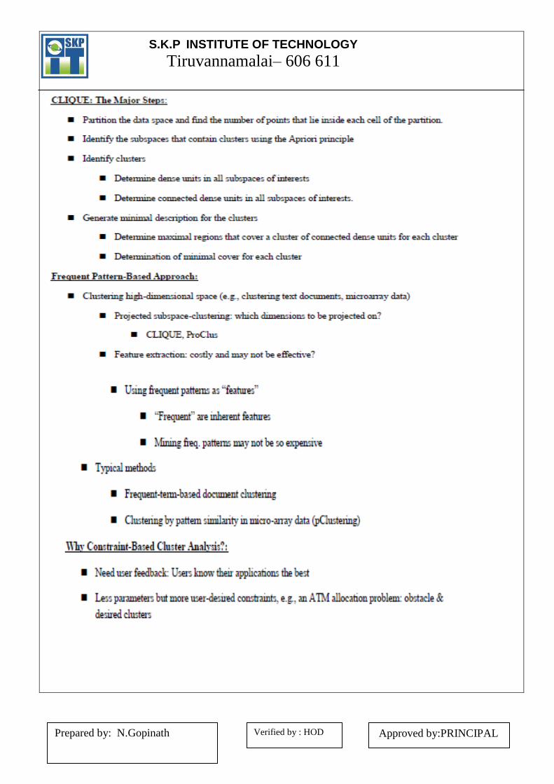
S.K.P INSTITUTE OF TECHNOLOGY Tiruvannamalai– 606 611
Verified by : HOD Prepared by: N.Gopinath
Approved by:PRINCIPAL

S.K.P INSTITUTE OF TECHNOLOGY Tiruvannamalai– 606 611
Verified by : HOD Prepared by: N.Gopinath
Approved by:PRINCIPAL

S.K.P INSTITUTE OF TECHNOLOGY Tiruvannamalai– 606 611
Verified by : HOD Prepared by: N.Gopinath
Approved by:PRINCIPAL

S.K.P INSTITUTE OF TECHNOLOGY Tiruvannamalai– 606 611
Verified by : HOD Prepared by: N.Gopinath
Approved by:PRINCIPAL