cs 380: artificial intelligence lecture...

1

CS 380: Artificial IntelligenceLecture #4

William Regli

Material

• Chapter 4 Section 1 - 3

2

Outline

• Best-first search• Greedy best-first search• A* search• Heuristics• Local search algorithms• Hill-climbing search• Simulated annealing search• Local beam search• Genetic algorithms

Review: Tree search

• A search strategy is defined by picking the order of node expansion

3

Best-first search• Idea: use an evaluation function f(n) for each node

– estimate of "desirability"Expand most desirable unexpanded node

• Implementation:Order the nodes in fringe in decreasing order of desirability

• Special cases:– greedy best-first search– A* search

Romania with step costs in km

4

Greedy best-first search

• Evaluation function f(n) = h(n) (heuristic)• = estimate of cost from n to goal• e.g., hSLD(n) = straight-line distance

from n to Bucharest• Greedy best-first search expands the

node that appears to be closest to goal

A heuristic function

• [dictionary]“A rule of thumb, simplification, or educated guess that reduces or limits the search for solutions in domains that are difficult and poorly understood.”– h(n) = estimated cost of the cheapest path from

node n to goal node.– If n is goal then h(n)=0

More information later.

5

Greedy best-first search example


6



7

Properties of greedy best-first search

• Complete?• Time?• Space?• Optimal?

Properties of greedy best-first search

• Complete? No – can get stuck in loops, e.g., Iasi Neamt Iasi Neamt

• Time? O(bm), but a good heuristic can give dramatic improvement

• Space? O(bm) -- keeps all nodes in memory

• Optimal? No

8

A* search

• Idea: avoid expanding paths that are already expensive

• Evaluation function f(n) = g(n) + h(n)• g(n) = cost so far to reach n• h(n) = estimated cost from n to goal• f(n) = estimated total cost of path

through n to goal

A* search example

9

A* search example

A* search example

10

A* search example

A* search example

11

A* search example

Admissible heuristics

• A heuristic h(n) is admissible if for every node n, h(n) ≤ h*(n), where h*(n) is the true cost to reach the goal state from n.

• An admissible heuristic never overestimatesthe cost to reach the goal, i.e., it is optimistic

• Example: hSLD(n) (never overestimates the actual road distance)

• Theorem: If h(n) is admissible, A* using TREE-SEARCH is optimal

12

Optimality of A* (proof)• Suppose some suboptimal goal G2 has been generated and is in

the fringe. Let n be an unexpanded node in the fringe such that n is on a shortest path to an optimal goal G.

• f(G2) = g(G2) since h(G2) = 0 • g(G2) > g(G) since G2 is suboptimal • f(G) = g(G) since h(G) = 0 • f(G2) > f(G) from above

Optimality of A* (proof)

• f(G2) > f(G) from above • h(n) ≤ h^*(n) since h is admissible• g(n) + h(n) ≤ g(n) + h*(n) • f(n) ≤ f(G)Hence f(G2) > f(n), and A* will never select G2 for expansion�

13

Consistent heuristics• A heuristic is consistent if for every node n, every successor n'

of n generated by any action a,

h(n) ≤ c(n,a,n') + h(n')

• If h is consistent, we havef(n') = g(n') + h(n')

= g(n) + c(n,a,n') + h(n') ≥ g(n) + h(n) = f(n)

• i.e., f(n) is non-decreasing along any path.• Theorem: If h(n) is consistent, A* using GRAPH-SEARCH is

optimal

Optimality of A*

• A* expands nodes in order of increasing f value• Gradually adds "f-contours" of nodes • Contour i has all nodes with f=fi, where fi < fi+1

14

Properties of A*

• Complete?• Time?• Space?• Optimal?

Properties of A*

• Complete? Yes (unless there are infinitely many nodes with f ≤ f(G) )

• Time? Exponential• Space? Keeps all nodes in memory• Optimal? Yes

15

Admissible heuristicsE.g., for the 8-puzzle:• h1(n) = number of misplaced tiles• h2(n) = total Manhattan distance(i.e., no. of squares from desired location of each tile)

• h1(S) = ? • h2(S) = ?

Admissible heuristicsE.g., for the 8-puzzle:�• h1(n) = number of misplaced tiles• h2(n) = total Manhattan distance(i.e., no. of squares from desired location of each tile)

• h1(S) = ? 8• h2(S) = ? 3+1+2+2+2+3+3+2 = 18

16

Dominance• If h2(n) ≥ h1(n) for all n (both admissible)• then h2 dominates h1• h2 is better for search

• Typical search costs (average number of nodes expanded):

• d=12 IDS = 3,644,035 nodesA*(h1) = 227 nodes A*(h2) = 73 nodes

• d=24 IDS = too many nodesA*(h1) = 39,135 nodes A*(h2) = 1,641 nodes

Relaxed problems• A problem with fewer restrictions on the

actions is called a relaxed problem• The cost of an optimal solution to a relaxed

problem is an admissible heuristic for the original problem

• If the rules of the 8-puzzle are relaxed so that a tile can move anywhere, then h1(n) gives the shortest solution

• If the rules are relaxed so that a tile can move to any adjacent square, then h2(n) gives the shortest solution

17

Memory Problems

Memory-bounded heuristic search

• Some solutions to A* space problems (maintain completeness and optimality)– Iterative-deepening A* (IDA*)

• Here cutoff information is the f-cost (g+h) instead of depth

– Recursive best-first search(RBFS)• Recursive algorithm that attempts to mimic standard

best-first search with linear space.

– (simple) Memory-bounded A* ((S)MA*)• Drop the worst-leaf node when memory is full

18

(simplified) memory-bounded A*

• Use all available memory.– I.e. expand best leafs until available memory is full– When full, SMA* drops worst leaf node (highest f-value)– Like RFBS backup forgotten node to its parent

• What if all leafs have the same f-value?– Same node could be selected for expansion and deletion.– SMA* solves this by expanding newest best leaf and deleting

oldest worst leaf.• SMA* is complete if solution is reachable, optimal if

optimal solution is reachable.

Recursive best-first search

• Keeps track of the f-value of the best-alternative path available. Call this f-limit.– (1) If current f-values exceeds f-limit than

backtrack to alternative path.– (2) When backtracking over a node, change its f-

value to best f-value of its children.• This is bookmarking for the future, in case we ever revisit

this node again.

19

Recursive best-first search, ex.

• Path until Rumnicu Vilcea is already expanded• Above node; f-limit for every recursive call is shown on top.• Below node: f(n)• The path is followed until Pitesti

– (1) Has a f-value worse than the f-limit. -> Backtrack


• (2) Backtrack over Rumnicu Vilcea and store f-value for best child (Pitesti w/ value 417 on previous slide)

• best is now Fagaras.– best child value is 450– (1) 450 is greater than 417 -> backtrack!

20


• Backtrack over Fagaras and store f-value for best child (bucharest=450)

• best is now Rimnicu Viclea (again).– Subtree is again expanded.– Best alternative subtree is now through Timisoara (447).

• Solution is found since because 447 > 417.

RBFS evaluation• RBFS is a bit more efficient than IDA*

– Still excessive node generation (mind changes)• Like A*, optimal if h(n) is admissible• Space complexity is O(bd).

– IDA* retains only one single number (the current f-cost limit)• Time complexity difficult to characterize

– Depends on accuracy if h(n) and how often best path changes.

• IDA* and RBFS suffer from too little memory.

21

Where do heuristics come from?

• Domain knowledge– straight line distance for a map– manhattan distance for 8-puzzle– pre-compute pattern databases (e.g., deep blue)

• Another key technique– Problem relaxation

• e.g., 8-puzzle, assume tiles can be moved anywhere

Local Search

22

Local search algorithms• In many optimization problems, the path to the goal is

irrelevant; the goal state itself is the solution

• State space = set of "complete" configurations• Find configuration satisfying constraints, e.g.,

n-queens

• In such cases, we can use local search algorithms• keep a single "current" state, try to improve it

Example: n-queens

• Put n queens on an n × n board with no two queens on the same row, column, or diagonal

23

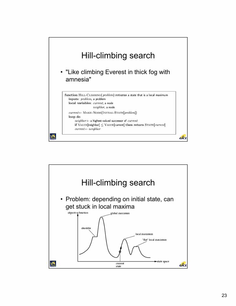
Hill-climbing search

• "Like climbing Everest in thick fog with amnesia"

Hill-climbing search

• Problem: depending on initial state, can get stuck in local maxima

24

Hill-climbing search: 8-queens problem

• h = number of pairs of queens that are attacking each other, either directly or indirectly

• h = 17 for the above state�

Hill-climbing search: 8-queens problem

• A local minimum with h = 1

25

Simulated annealing search

• Idea: escape local maxima by allowing some "bad" moves but gradually decrease their frequency

Properties of simulated annealing search

• One can prove: If T decreases slowly enough, then simulated annealing search will find a global optimum with probability approaching 1

• Widely used in VLSI layout, airline scheduling, etc

26

Simulated Annealing History

Local beam search

• Keep track of k states rather than just one

• Start with k randomly generated states

• At each iteration, all the successors of all kstates are generated

• If any one is a goal state, stop; else select the k best successors from the complete list and repeat.

27

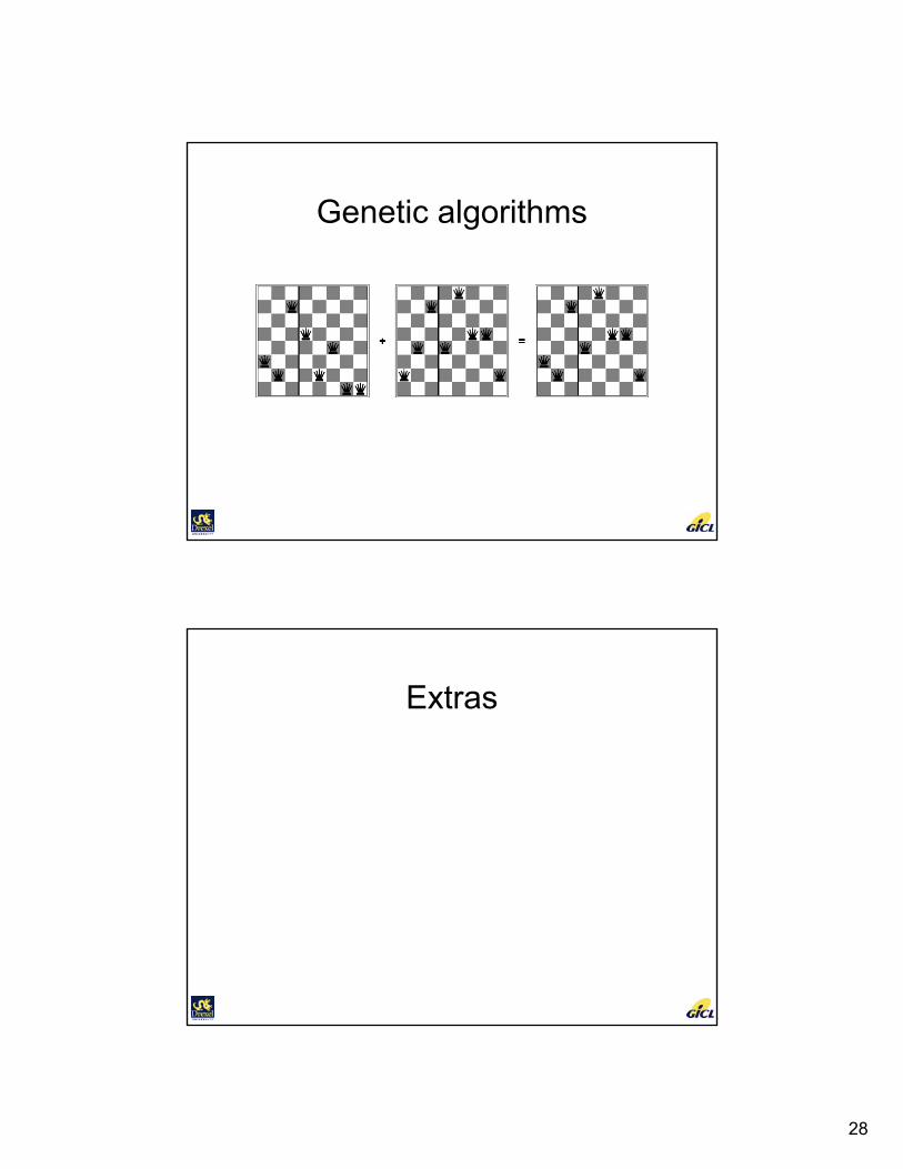
Genetic algorithms• A successor state is generated by combining two parent states

• Start with k randomly generated states (population)

• A state is represented as a string over a finite alphabet (often a string of 0s and 1s)

• Evaluation function (fitness function). Higher values for better states.

• Produce the next generation of states by selection, crossover, and mutation

Genetic algorithms

• Fitness function: number of non-attacking pairs of queens (min = 0, max = 8 × 7/2 = 28)

• 24/(24+23+20+11) = 31%• 23/(24+23+20+11) = 29% etc

28

Genetic algorithms

Extras

29

Memory-bounded heuristic search

• Some solutions to A* space problems (maintain completeness and optimality)– Iterative-deepening A* (IDA*)

• Here cutoff information is the f-cost (g+h) instead of depth

– Recursive best-first search(RBFS)• Recursive algorithm that attempts to mimic standard

best-first search with linear space.

– (simple) Memory-bounded A* ((S)MA*)• Drop the worst-leaf node when memory is full

Recursive best-first searchfunction RECURSIVE-BEST-FIRST-SEARCH(problem) return a solution or

failurereturn RFBS(problem,MAKE-NODE(INITIAL-STATE[problem]),∞)

function RFBS( problem, node, f_limit) return a solution or failure and a new f-cost limitif GOAL-TEST[problem](STATE[node]) then return nodesuccessors ← EXPAND(node, problem)if successors is empty then return failure, ∞for each s in successors do

f [s] ← max(g(s) + h(s), f [node])repeat

best ← the lowest f-value node in successorsif f [best] > f_limit then return failure, f [best]alternative ← the second lowest f-value among successorsresult, f [best] ← RBFS(problem, best, min(f_limit, alternative))if result ≠ failure then return result

30

Recursive best-first search

• Keeps track of the f-value of the best-alternative path available.– If current f-values exceeds this alternative

f-value than backtrack to alternative path.– Upon backtracking change f-value to best

f-value of its children.– Re-expansion of this result is thus still

possible.


• Path until Rumnicu Vilcea is already expanded• Above node; f-limit for every recursive call is shown

on top.• Below node: f(n)• The path is followed until Pitesti which has a f-value

worse than the f-limit.

31


• Unwind recursion and store best f-value for current best leaf Pitesti

result, f [best] ← RBFS(problem, best, min(f_limit, alternative))

• best is now Fagaras. Call RBFS for new best– best value is now 450


• Unwind recursion and store best f-value for current best leaf Fagaras

result, f [best] ← RBFS(problem, best, min(f_limit, alternative))

• best is now Rimnicu Viclea (again). Call RBFS for new best– Subtree is again expanded.– Best alternative subtree is now through Timisoara.

• Solution is found since because 447 > 417.

32

RBFS evaluation

• RBFS is a bit more efficient than IDA*– Still excessive node generation (mind changes)

• Like A*, optimal if h(n) is admissible• Space complexity is O(bd).

– IDA* retains only one single number (the current f-cost limit)

• Time complexity difficult to characterize– Depends on accuracy if h(n) and how often best

path changes.• IDA* en RBFS suffer from too little memory.

(simplified) memory-bounded A*

• Use all available memory.– I.e. expand best leafs until available memory is full– When full, SMA* drops worst leaf node (highest f-value)– Like RFBS backup forgotten node to its parent

• What if all leafs have the same f-value?– Same node could be selected for expansion and deletion.– SMA* solves this by expanding newest best leaf and deleting

oldest worst leaf.• SMA* is complete if solution is reachable, optimal if

optimal solution is reachable.

cs 380: artificial intelligence lecture...

Documents