CS-184: Computer Graphics Lecture #21: Fluid Simulation II

Rahul NarainUniversity of California, Berkeley!Nov. 18–19, 2013

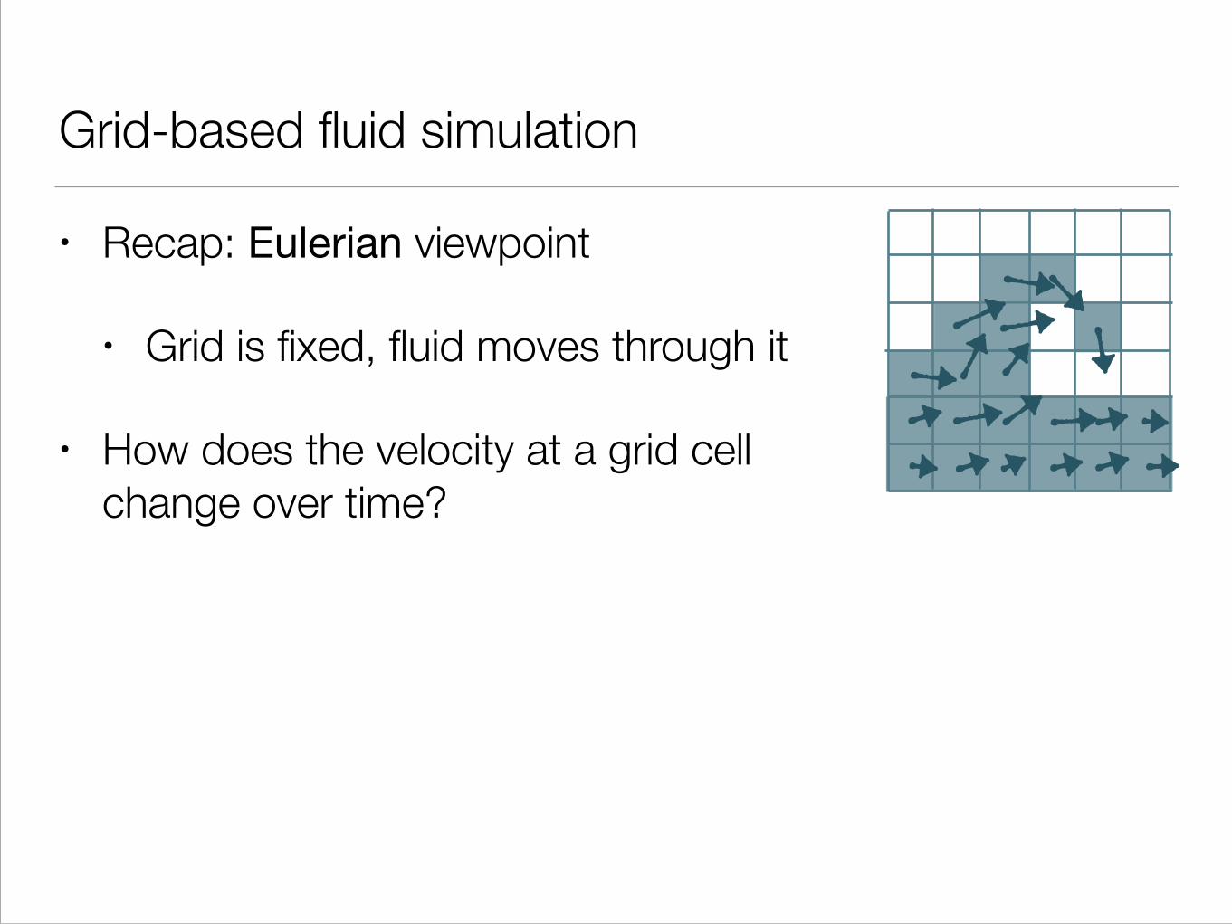
Grid-based fluid simulation

• Recap: Eulerian viewpoint

• Grid is fixed, fluid moves through it

• How does the velocity at a grid cell change over time?

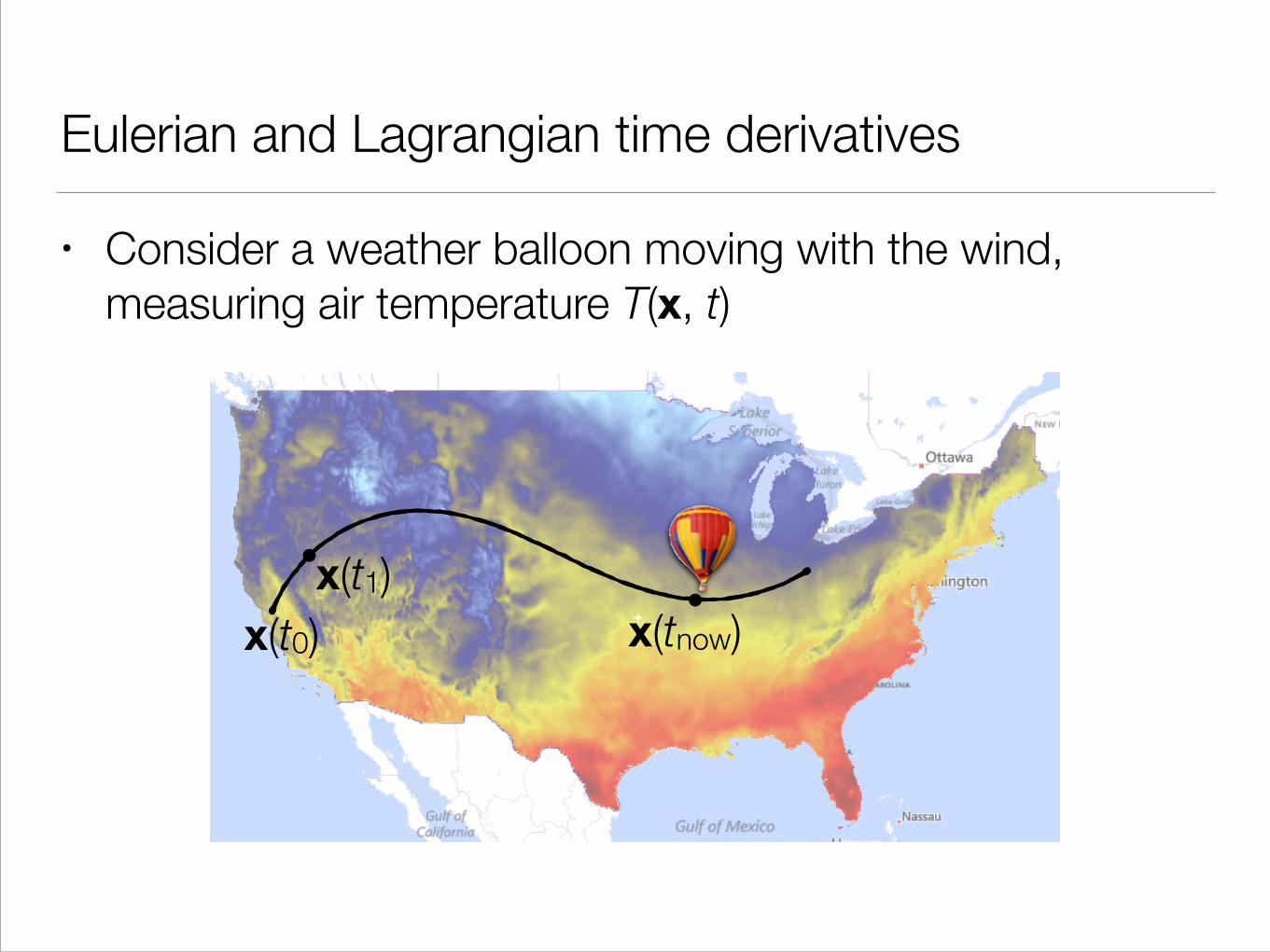
Eulerian and Lagrangian time derivatives

• Consider a weather balloon moving with the wind, measuring air temperature T(x, t)

x(t0)x(t1)

x(tnow)

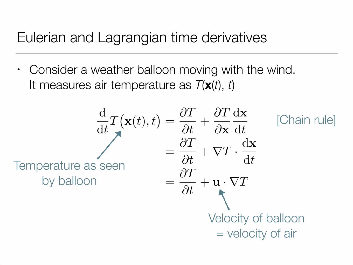
Eulerian and Lagrangian time derivatives

• Consider a weather balloon moving with the wind. It measures air temperature as T(x(t), t)

d

dtT�x(t), t

�=

@T

@t+

@T

@x

dx

dt

=@T

@t+rT · dx

dt

=@T

@t+ u ·rT

Temperature as seenby balloon

[Chain rule]

Velocity of balloon= velocity of air

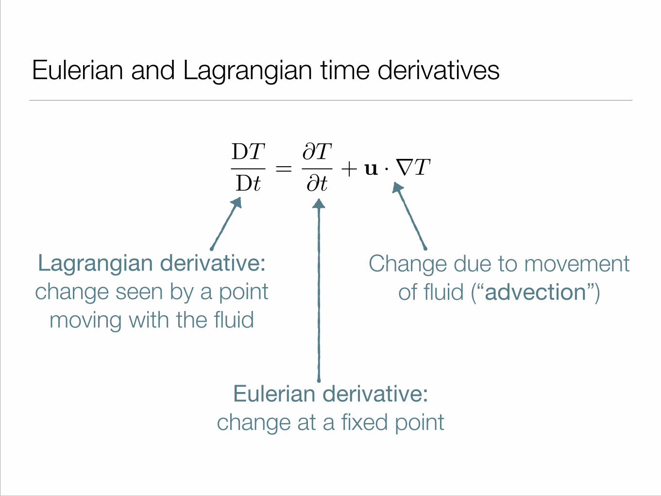
Eulerian and Lagrangian time derivatives

DT

Dt=

@T

@t+ u ·rT

Lagrangian derivative:change seen by a point

moving with the fluid

Change due to movementof fluid (“advection”)

Eulerian derivative:change at a fixed point

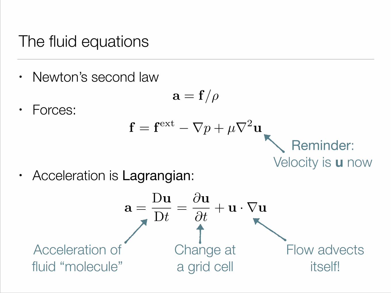
The fluid equations

• Newton’s second law

• Forces:

!

• Acceleration is Lagrangian:

a = f/⇢

f = f ext �rp+ µr2uReminder:

Velocity is u now

a =Du

Dt=

@u

@t+ u ·ru

Acceleration offluid “molecule”

Change ata grid cell

Flow advectsitself!

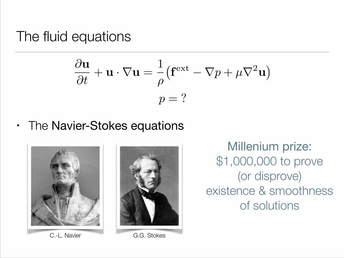
The fluid equations

!

!

• The Navier-Stokes equations

@u

@t+ u ·ru =

1

⇢

�f ext �rp+ µr2u

�

p = ?

C.-L. Navier G.G. Stokes

Millenium prize:$1,000,000 to prove

(or disprove)existence & smoothness

of solutions

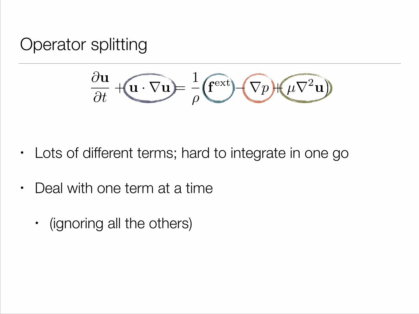
Operator splitting

!

!

• Lots of different terms; hard to integrate in one go

• Deal with one term at a time

• (ignoring all the others)

@u

@t+ u ·ru =

1

⇢

�f ext �rp+ µr2u

�

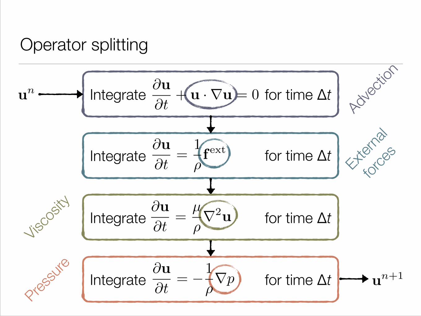
Operator splitting

un

un+1

@u

@t+ u ·ru = 0Integrate for time Δt

Advec

tion

@u

@t=

1

⇢f extIntegrate for time Δt Exte

rnal

force

s

@u

@t= �1

⇢rpIntegrate for time Δt

Pressur

e

Viscos

ityIntegrate for time Δt

@u

@t=

µ

⇢r2u

Advection

!

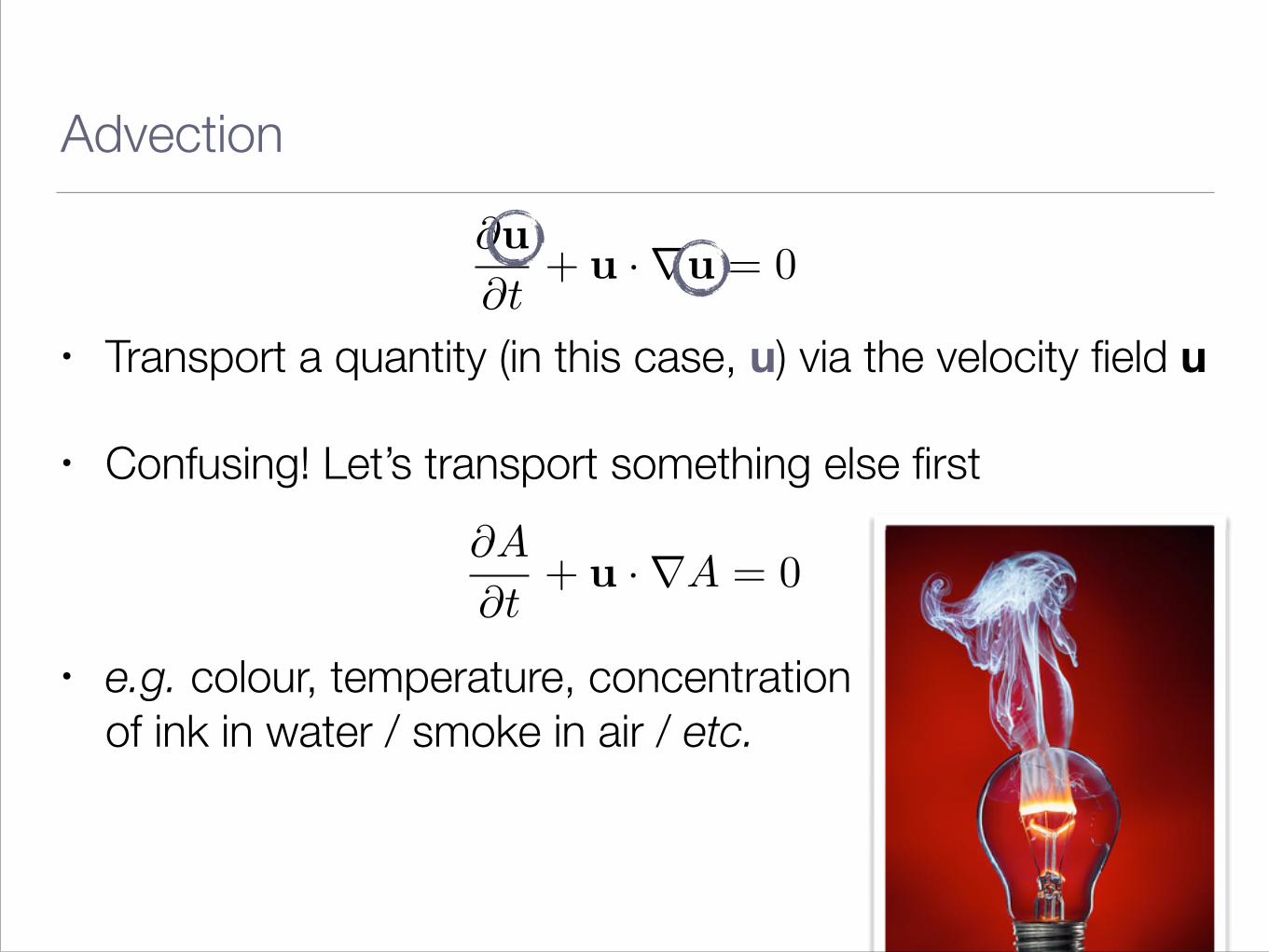
• Transport a quantity (in this case, u) via the velocity field u

• Confusing! Let’s transport something else first

!

• e.g. colour, temperature, concentration of ink in water / smoke in air / etc.

@u

@t+ u ·ru = 0

@A

@t+ u ·rA = 0

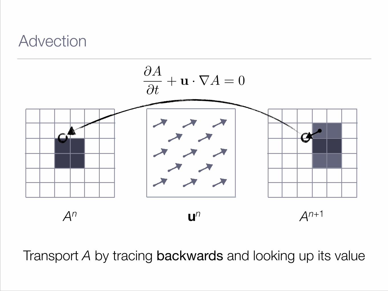
Advection

An An+1un

@A

@t+ u ·rA = 0

Transport A by tracing backwards and looking up its value

Advection

• Input: initial grid An, velocity field un

• Output: final grid An+1

• For each grid cell xi

• Backtrace position, e.g.

• Set output

x

back = xi � ui�t

An+1i = interpolate An

at x

back

To advect velocities, just feed in un as the initial grid too.

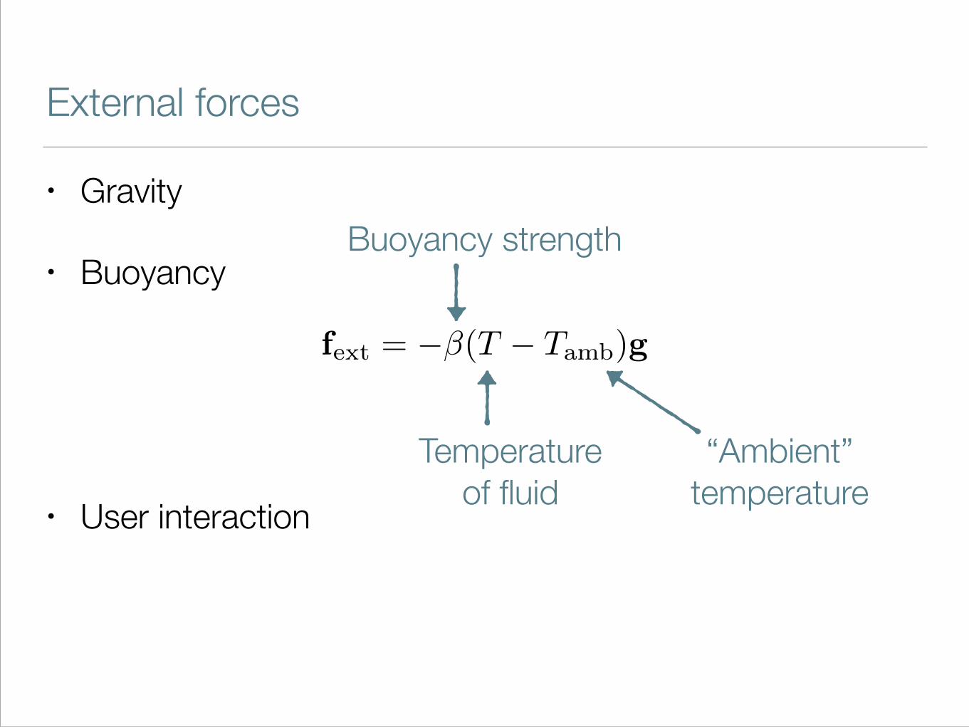
External forces

• Gravity

• Buoyancy

!

!

• User interaction

fext

= ��(T � Tamb

)g

Buoyancy strength

Temperatureof fluid

“Ambient”temperature

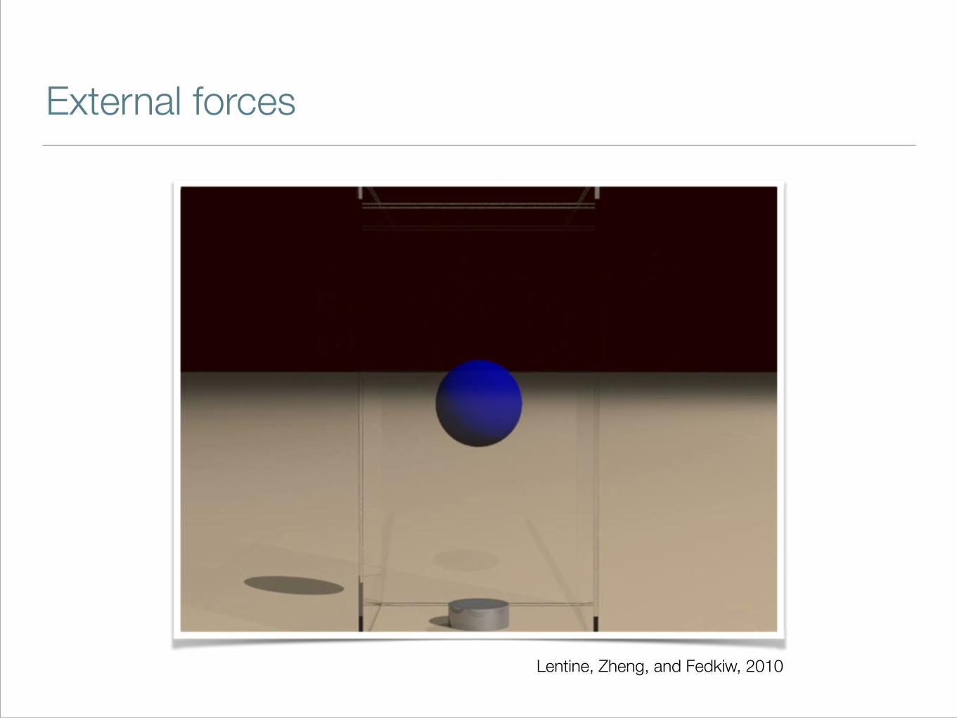
External forces

Lentine, Zheng, and Fedkiw, 2010

Pressure

Becker and Teschner, 2007

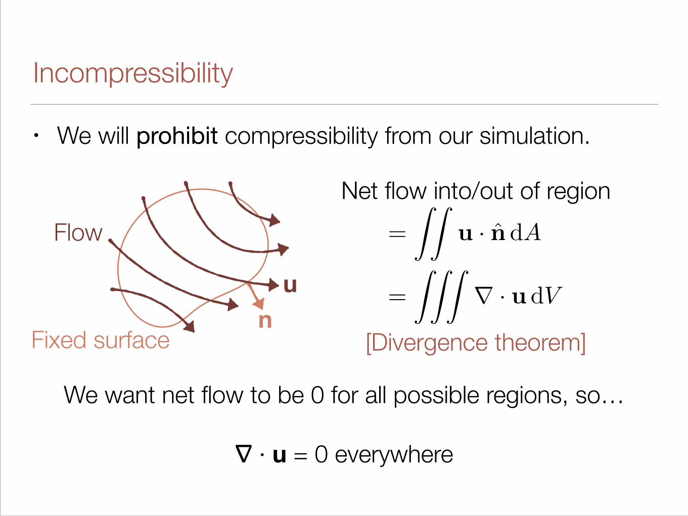
Incompressibility

• We will prohibit compressibility from our simulation.

n

Net flow into/out of region=

ZZu · n̂ dA

=

ZZZr · u dV

[Divergence theorem]

We want net flow to be 0 for all possible regions, so… !

∇ · u = 0 everywhere

Fixed surface

u

Flow

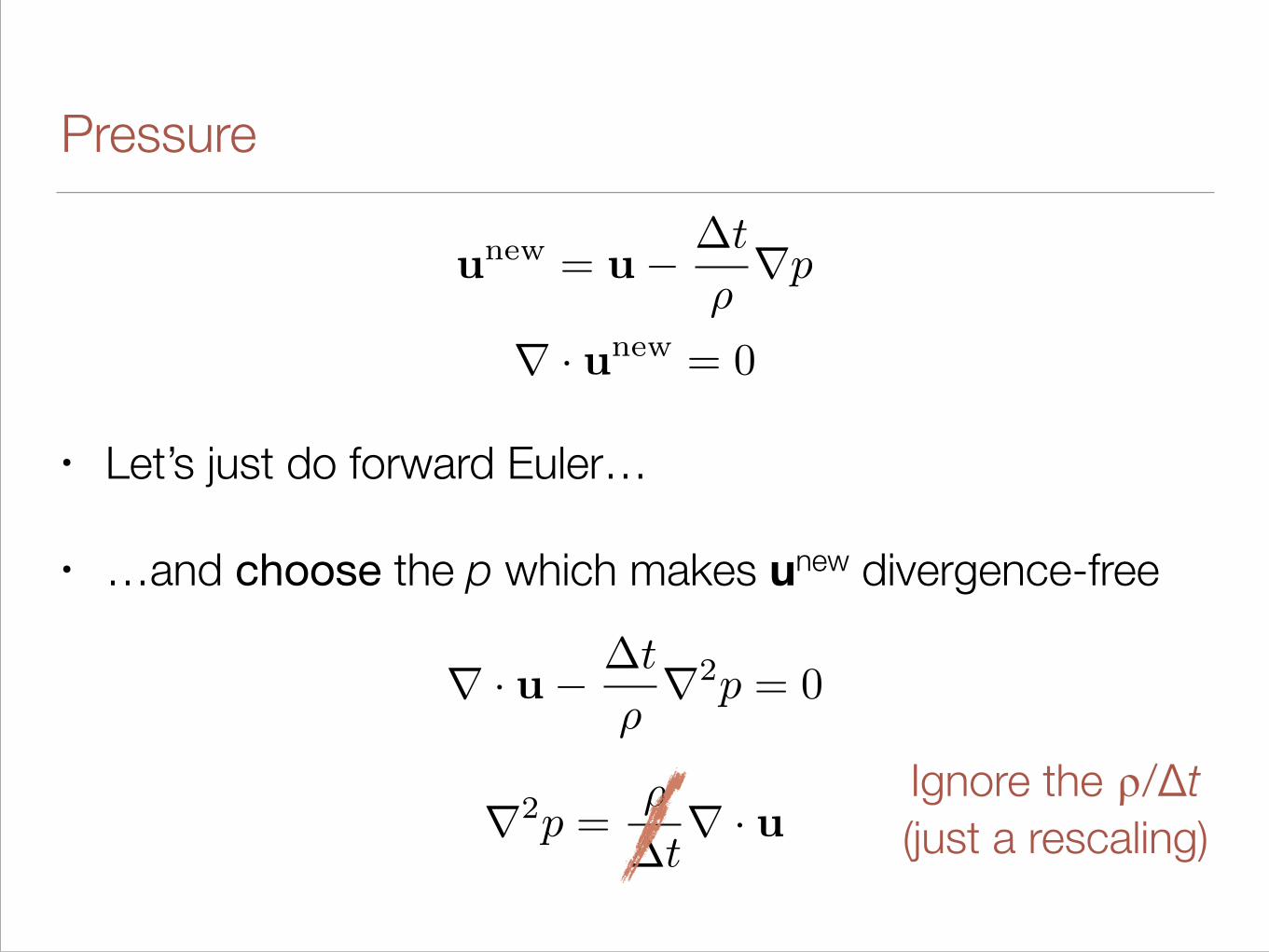
Pressure

!

!

• Let’s just do forward Euler…

@u

@t= �1

⇢rp

p = ?

Pressure

!

!

• Let’s just do forward Euler…

• …and choose the p which makes unew divergence-free

unew = u� �t

⇢rp

r · unew = 0

r · u� �t

⇢r2p = 0

r2p =⇢

�tr · u

Ignore the ⍴/Δt(just a rescaling)

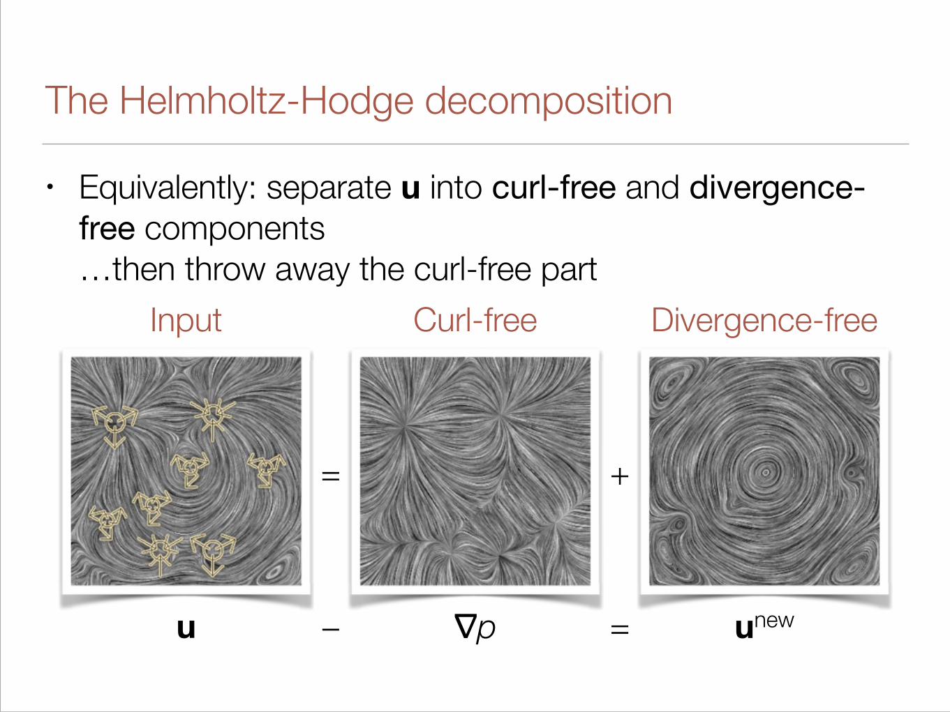
The Helmholtz-Hodge decomposition

• Equivalently: separate u into curl-free and divergence-free components…then throw away the curl-free part

= +

Input Curl-free Divergence-free

u ∇p unew− =

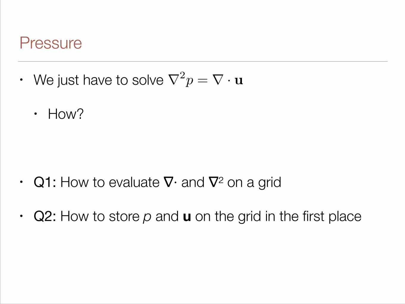
Pressure

• We just have to solve

• How?

!

• Q1: How to evaluate ∇· and ∇² on a grid

• Q2: How to store p and u on the grid in the first place

r2p = r · u

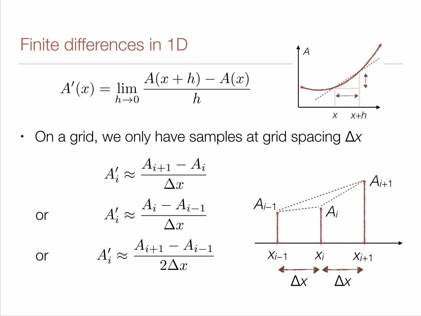
Finite differences in 1D

• On a grid, we only have samples at grid spacing Δx

A

0(x) = limh!0

A(x+ h)�A(x)

h

x x+h

A

A

0i ⇡

Ai+1 �Ai

�x

A

0i ⇡

Ai �Ai�1

�x

or

A

0i ⇡

Ai+1 �Ai�1

2�x

or xi xi+1xi−1

Ai−1 Ai

Ai+1

Δx Δx

Finite differences in 2D

• Apply forward and backward differences

r2A =

@

2A

@x

2+

@

2A

@y

2

⇣@

2A

@x

2

⌘

i,j⇡ Ai�1,j � 2Ai,j +Ai+1,j

�x

2

⇣@

2A

@y

2

⌘

i,j⇡ Ai,j�1 � 2Ai,j +Ai,j+1

�x

2

+1 -2 +1

+1

-2

+1

+1

+1 -4 +1

+1

Five point stencil for the Laplacian

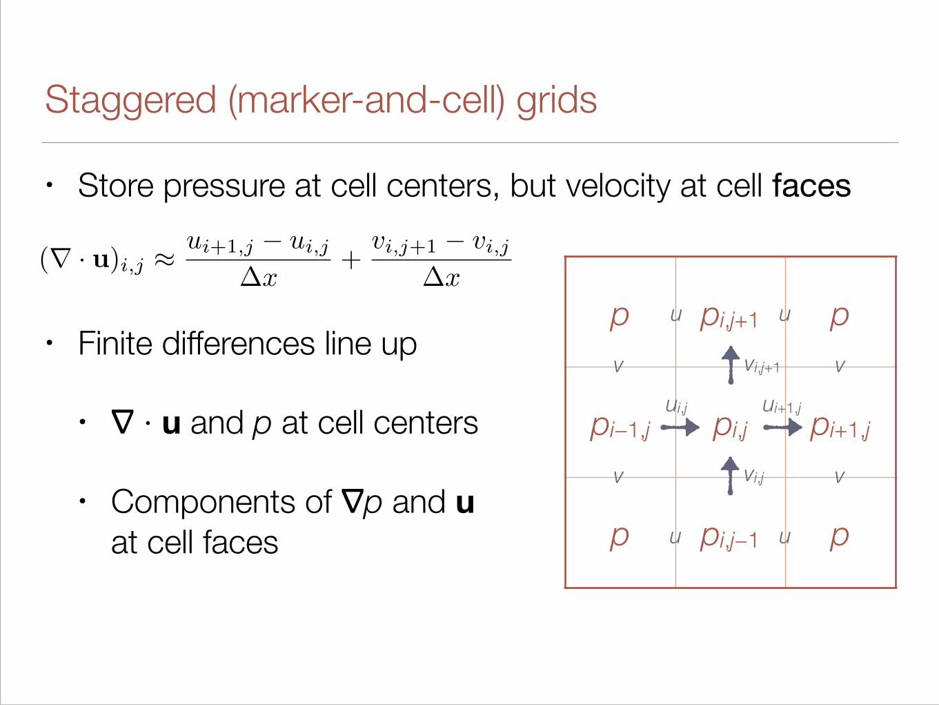
Staggered (marker-and-cell) grids

• Store pressure at cell centers, but velocity at cell faces

!

• Finite differences line up

• ∇ · u and p at cell centers

• Components of ∇p and uat cell faces

p pi,j+1 p

pi−1,j pi,j pi+1,j

p pi,j−1 p

ui+1,jui,j

vi,j

vi,j+1v v

v v

uu

uu

(r · u)i,j ⇡ui+1,j � ui,j

�x

+vi,j+1 � vi,j

�x

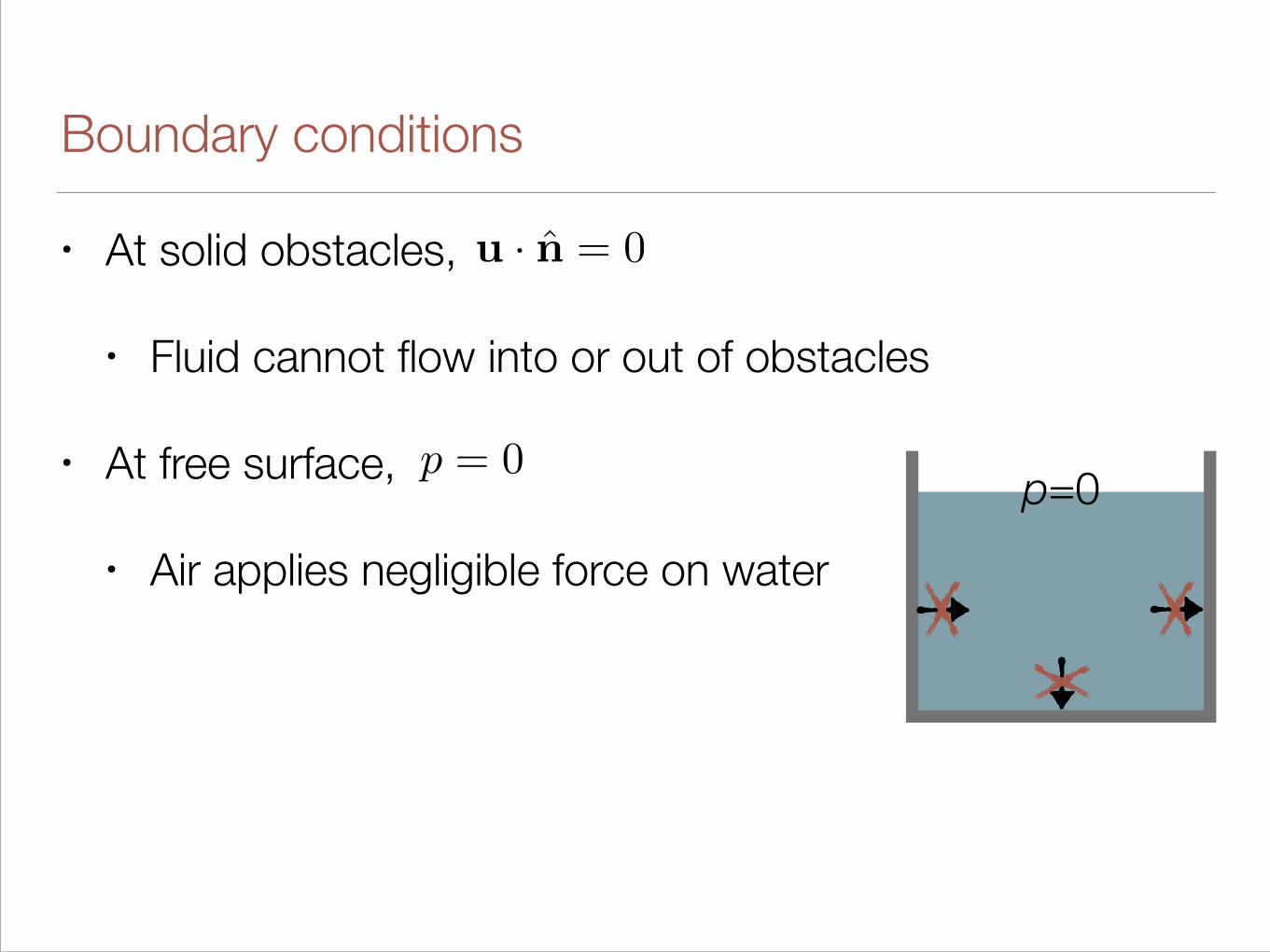
Boundary conditions

• At solid obstacles,

• Fluid cannot flow into or out of obstacles

• At free surface,

• Air applies negligible force on water

u · n̂ = 0

p = 0 p=0

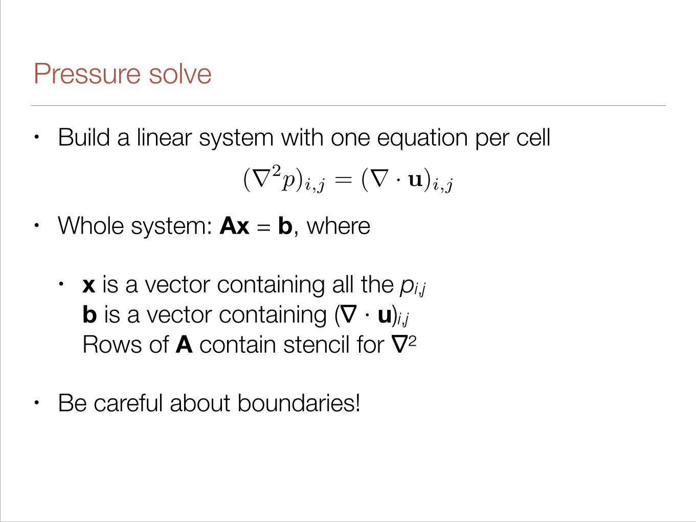
Pressure solve

• Build a linear system with one equation per cell

• Whole system: Ax = b, where

• x is a vector containing all the pi,jb is a vector containing (∇ · u)i,jRows of A contain stencil for ∇²

• Be careful about boundaries!

(r2p)i,j = (r · u)i,j

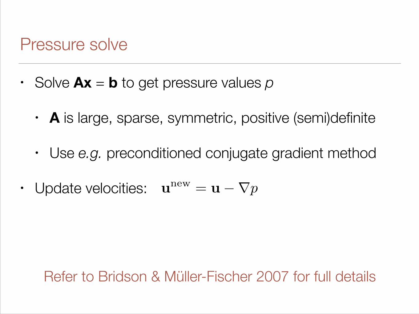
Pressure solve

• Solve Ax = b to get pressure values p

• A is large, sparse, symmetric, positive (semi)definite

• Use e.g. preconditioned conjugate gradient method

• Update velocities: unew = u�rp

Refer to Bridson & Müller-Fischer 2007 for full details

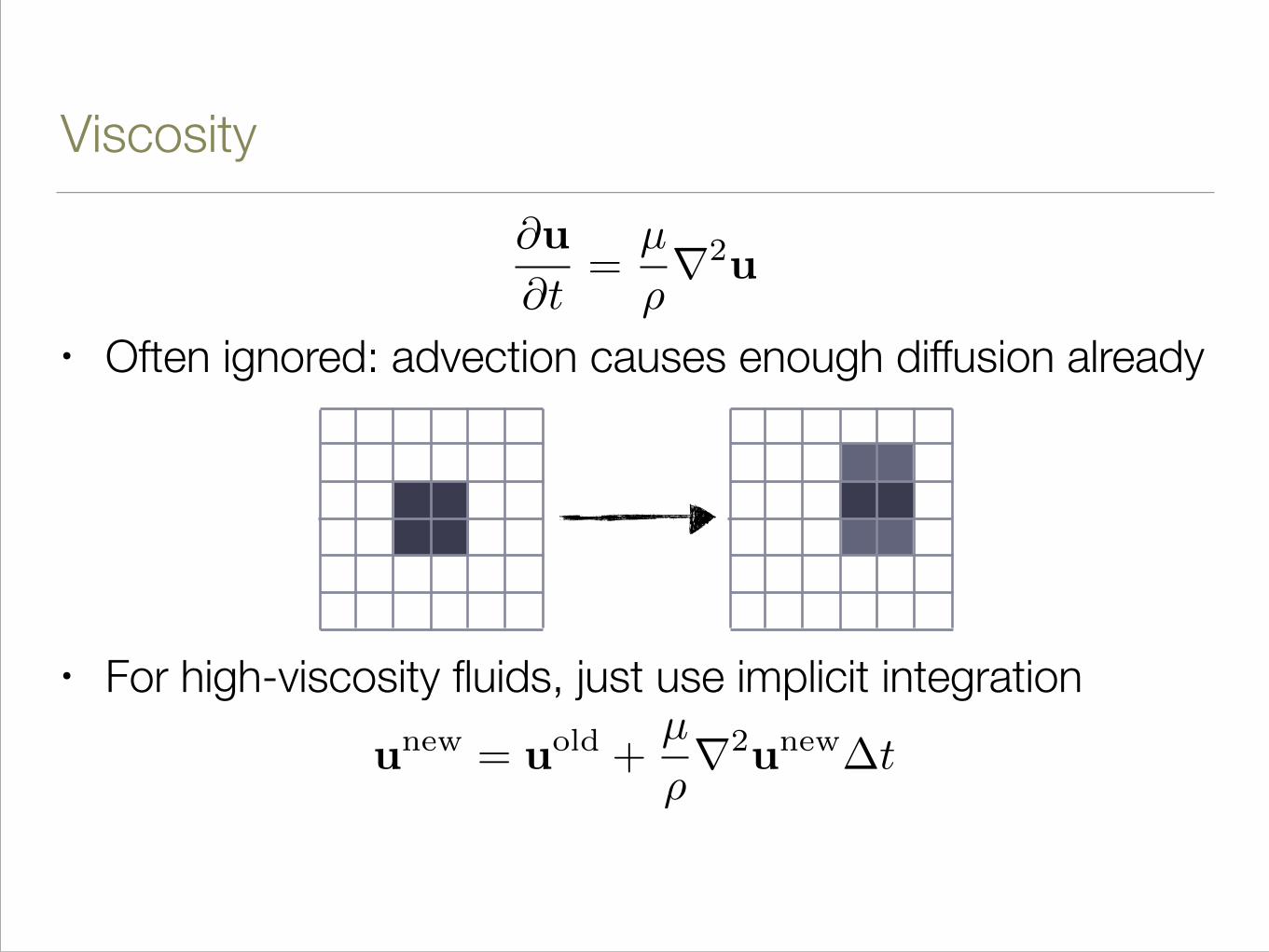
Viscosity

!

• Often ignored: advection causes enough diffusion already

!

!

• For high-viscosity fluids, just use implicit integration

@u

@t=

µ

⇢r2u

unew = uold +µ

⇢r2unew�t

Viscosity

Carlson, Mucha, Van Horn, and Turk, 2002

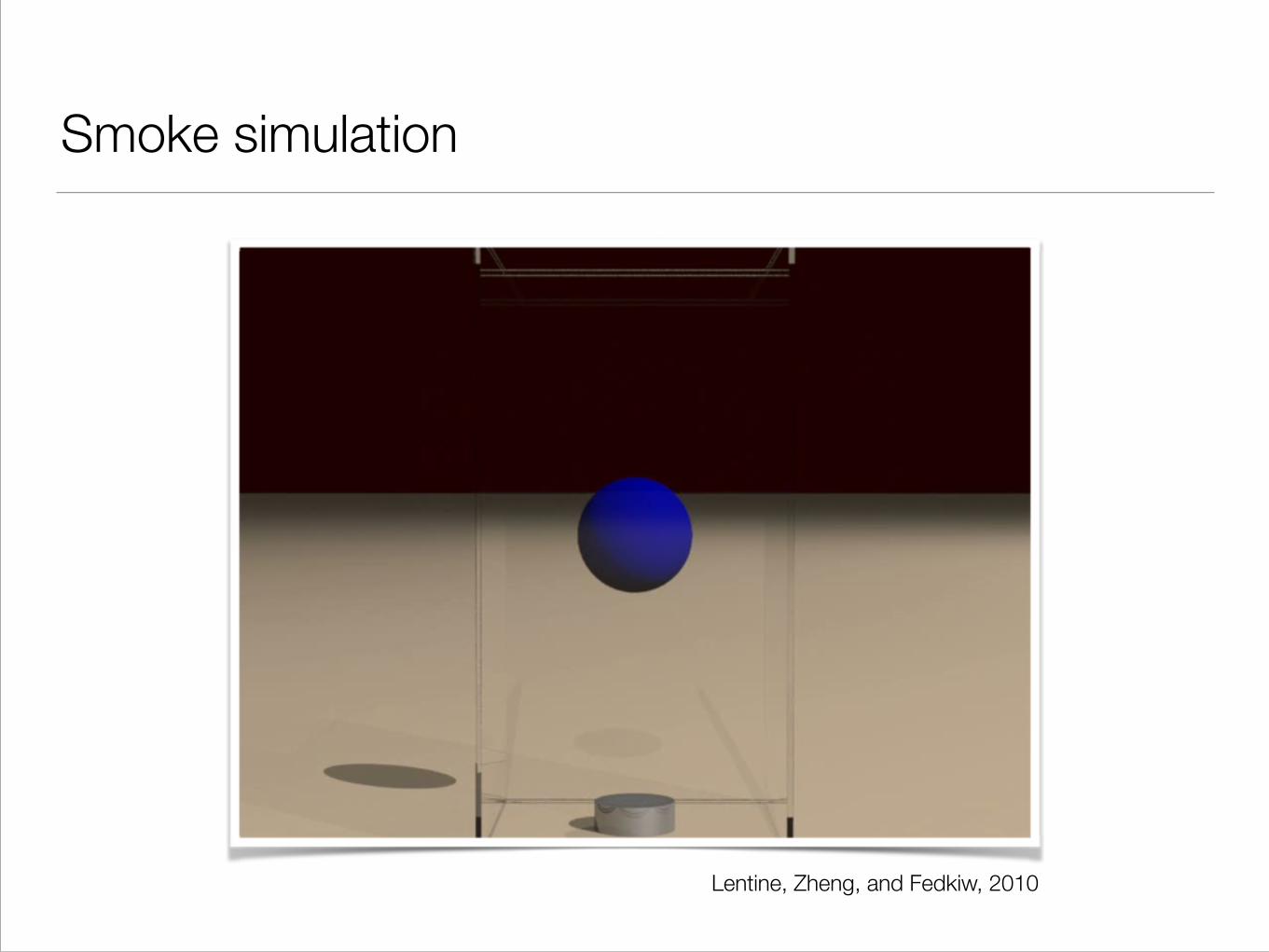
Smoke simulation

Lentine, Zheng, and Fedkiw, 2010

Surface tracking

• How to represent the surface of a liquid?

Option 1: Level set method

• Store the signed distance to surface φ(x) on grid cells

• Advect forward at each time step

• Surface is the level set (isosurface)at φ = 0

Surface tracking

• How to represent the surface of a liquid?

Option 2: Particles (easier)

• Keep lots of particles in the fluid, passively advected with the flow

• Reconstruct surface as in SPH

Zhu and Bridson, 2005

More options: level set + particles, volume-of-fluid, meshes, …

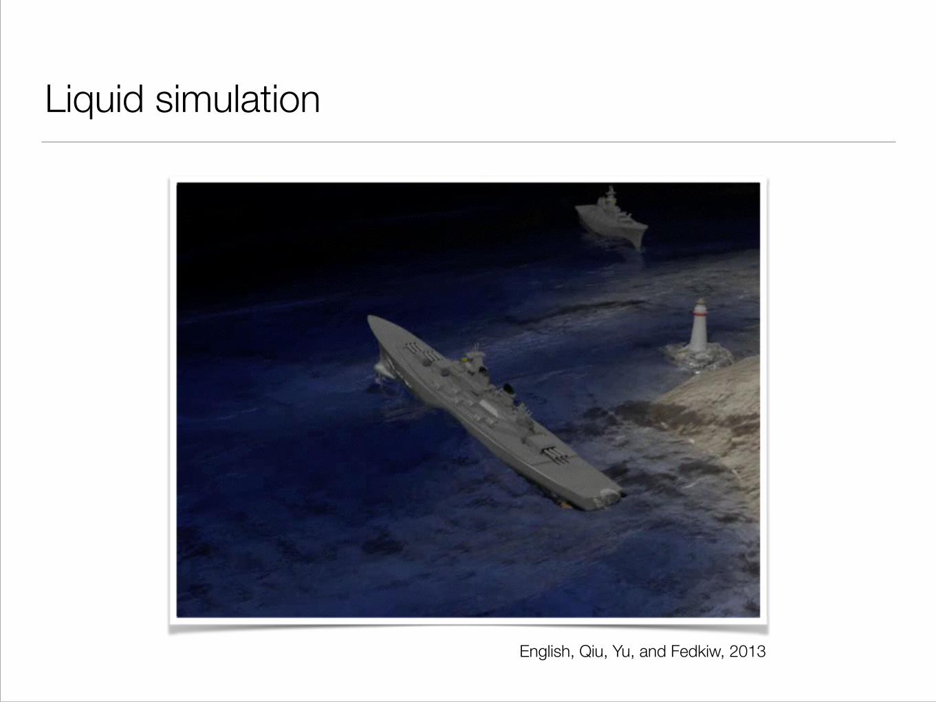
Liquid simulation

English, Qiu, Yu, and Fedkiw, 2013

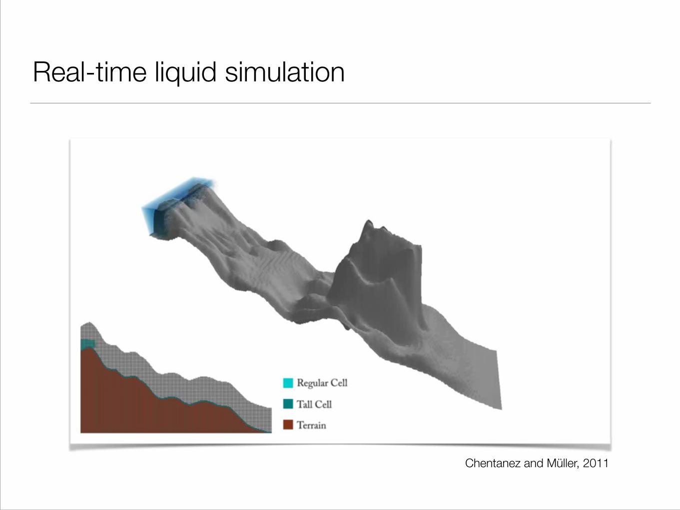
Real-time liquid simulation

Chentanez and Müller, 2011

References

• Bridson and Müller-Fischer, “Fluid Simulation for Computer Animation”, SIGGRAPH 2007 course notes

• Stam, “Stable Fluids”, 1999

• Enright, Marschner, and Fedkiw, “Animation and Rendering of Complex Water Surfaces”, 2002

• Zhu and Bridson, “Animating Sand as a Fluid”, 2005(for particle-based surface tracking, and more)