cs 128/es 228 - lecture 9a1 principles of remote sensing image from nasa – goddard space flight...

CS 128/ES 228 - Lecture 9a 1

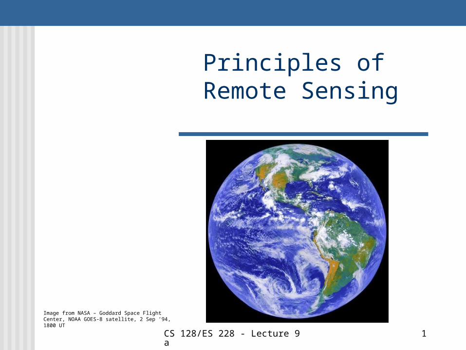
Principles of Remote Sensing

Image from NASA – Goddard Space Flight Center, NOAA GOES-8 satellite, 2 Sep ’94, 1800 UT


Scanning planet Earth from space


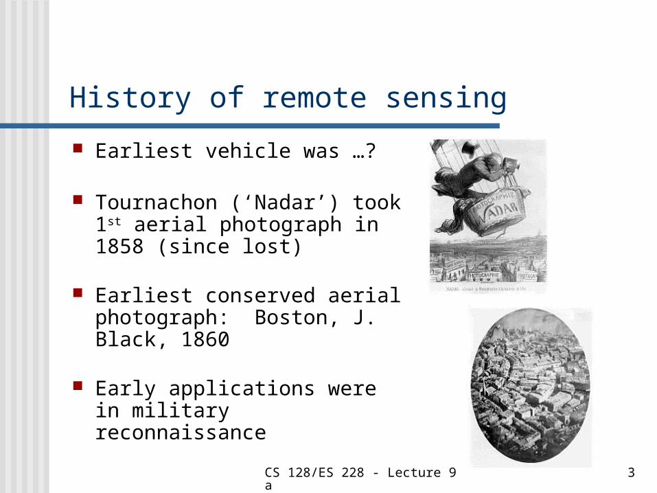
History of remote sensing

Earliest vehicle was …?

Tournachon (‘Nadar’) took 1st aerial photograph in 1858 (since lost)

Earliest conserved aerial photograph: Boston, J. Black, 1860

Early applications were in military reconnaissance


WWII – heavy use of aerial reconnaissance

Images: Avery. 1977. Interpretation of Aerial Photographs. 3rd ed. Burgess Press, Minneapolis, MN.


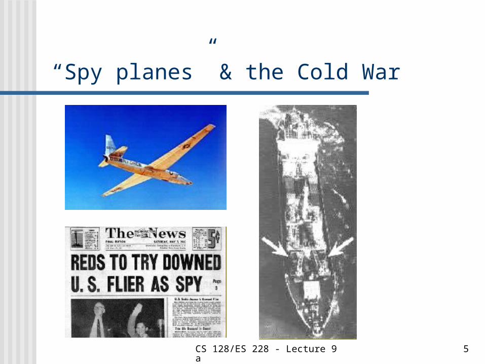
“Spy planes” & the Cold War


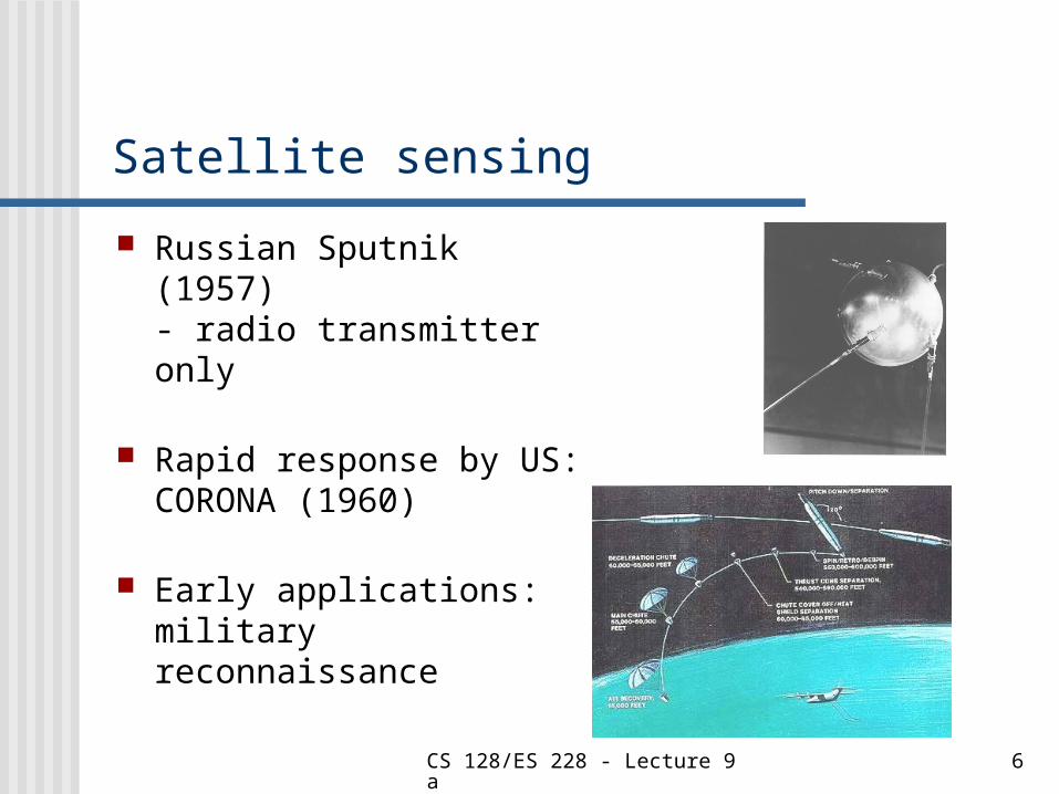
Satellite sensing

Russian Sputnik (1957)- radio transmitter only

Rapid response by US:CORONA (1960)

Early applications: military reconnaissance


Advantages of satellites

Wide coverage

Vertical (orthogonal) view

Multi-spectral data bands

Rapid data collection


Sources of EM radiation

Key distinction: passive sensing active sensing

Spectral ‘signatures”

Top: Lo & Yeung, fig. 8.1 Bottom: ASTER Spectral Library (http://speclib.jpl.nasa.gov)


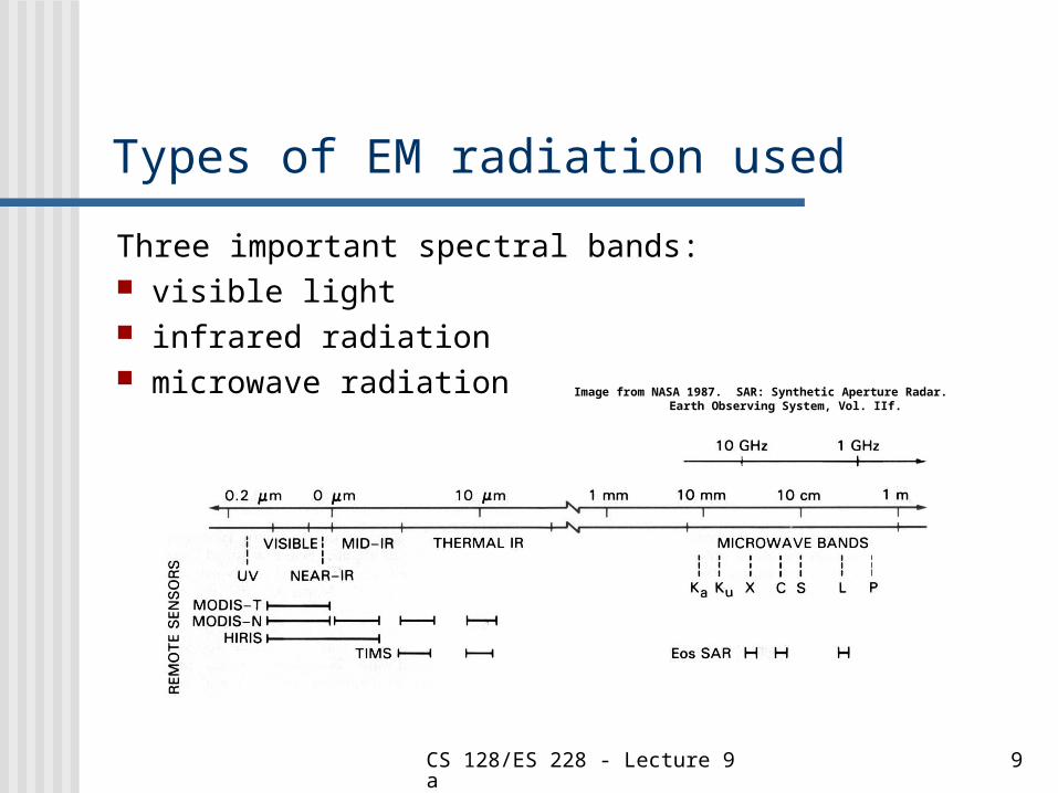
Types of EM radiation used

Three important spectral bands: visible light infrared radiation microwave radiation Image from NASA 1987. SAR: Synthetic Aperture Radar.

Earth Observing System, Vol. IIf.


Atmospheric attenuation

Scattering caused by aerosols

(water vapor, dust, smoke)

more intense at shorter wavelengths

why the sky is blue

Absorption caused by gas

molecules (H2O, CO2, O2, O3)

each molecule absorbs at a specific wave-length

result: atmospheric transmission windows


Transmission windows

UV-visible-IR

Microwave

Image from NASA 1987. From Pattern to Process: The Strategy of the Earth Observing System. Vol. II.


Classes of sensors

Photographic panchromatic color

Infrared (IR) film (near IR) thermal IR sensors

for longer wave-lengths

Multi-spectral scanners sensors for many wavelengths image scanned across sensors

Radar RAdio Detection

And Ranging

active imaging


Visual sensors: film types

panchromatic

near-infrared

color

Both images from Committee on Earth Observation Satellites http://ceos.cnes.fr:8100/cdrom-98/ceos1/irsd/content.htm


Infrared sensors

IR penetrates haze and light cloud cover

can be used at night

used by military for camouflage detection

IR ‘signature’ often distinct from visible image


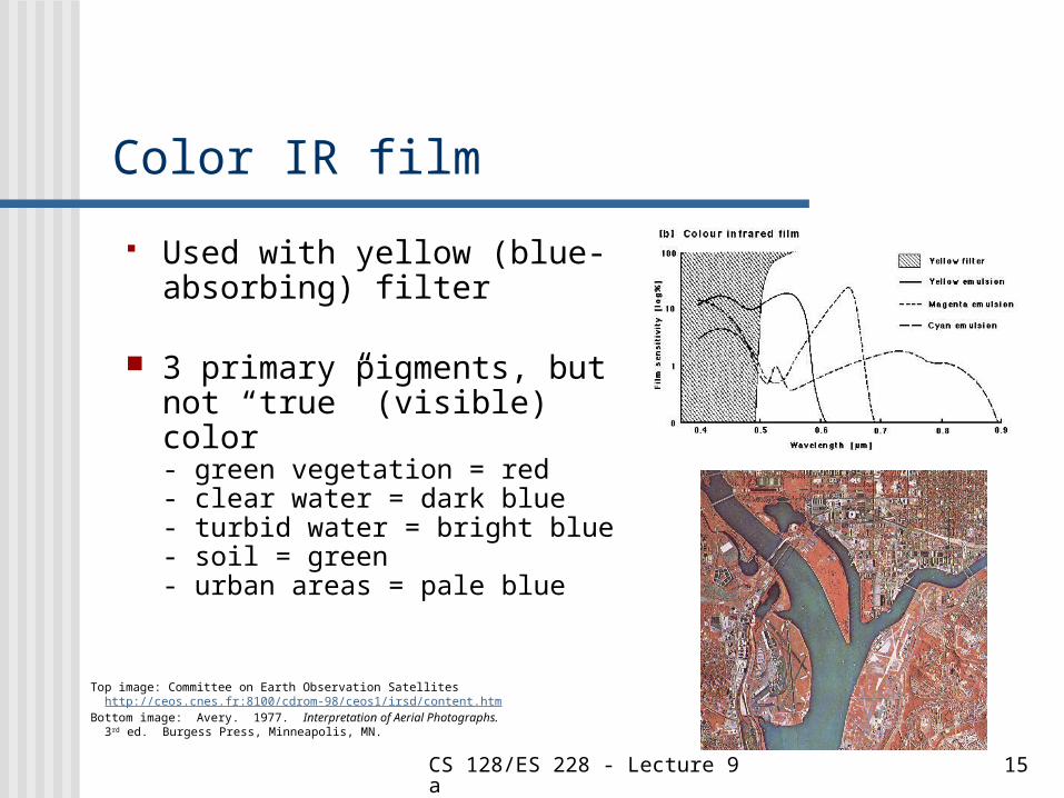
Color IR film

Used with yellow (blue-absorbing) filter

3 primary pigments, but not “true” (visible) color - green vegetation = red- clear water = dark blue- turbid water = bright blue- soil = green- urban areas = pale blue

Top image: Committee on Earth Observation Satellites http://ceos.cnes.fr:8100/cdrom-98/ceos1/irsd/content.htmBottom image: Avery. 1977. Interpretation of Aerial Photographs. 3rd ed. Burgess Press, Minneapolis, MN.


Multispectral sensors Visible + IR spectra

Comparison of film and electronic sensor spectral bands

Top: Avery 1977. Interpretation of Aerial Photography. Burgess Publ., NinneapolisBottom: ASTER Science page (http://www.science.aster.ersdac.or.jp/users/parte1/02-5.htm#3)


Radar sensors

active sensing

day & night, all weather

less affected by scattering (aerosols)

vertical or oblique perspective

Lo & Yeung, fig. 8.13


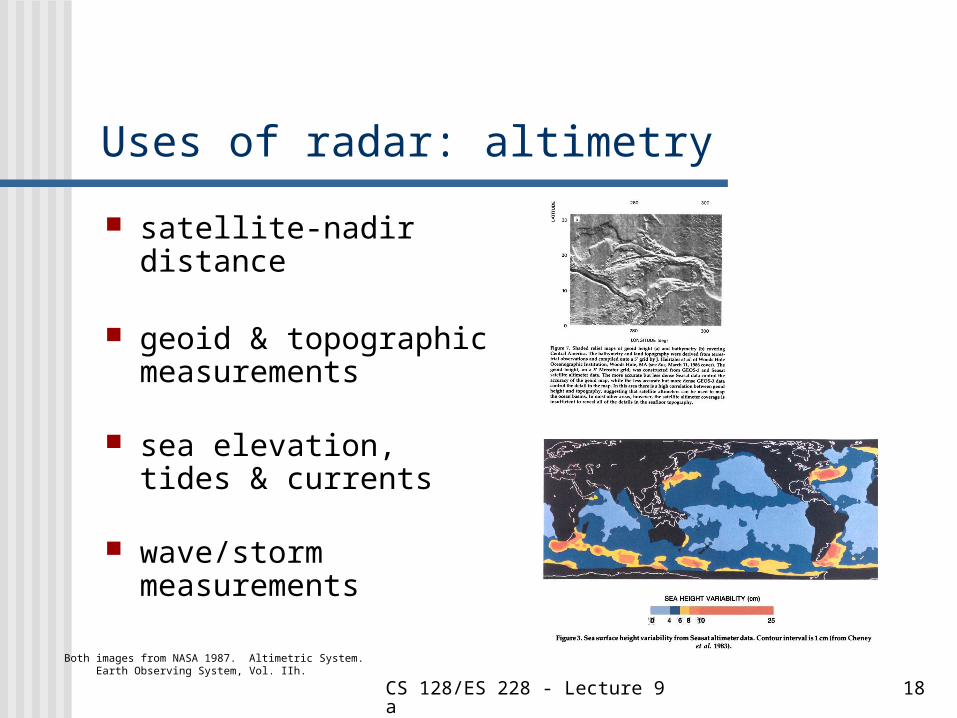
Uses of radar: altimetry

satellite-nadir distance

geoid & topographic measurements

sea elevation, tides & currents

wave/storm measurements

Both images from NASA 1987. Altimetric System. Earth Observing System, Vol. IIh.


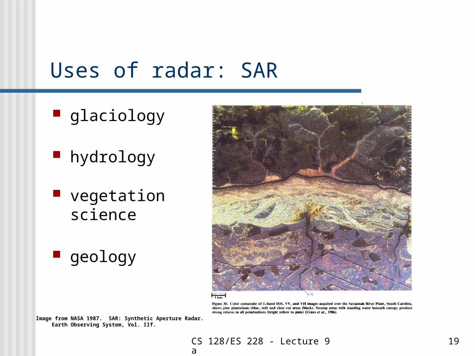
Uses of radar: SAR

glaciology

hydrology

vegetation science

geology

Image from NASA 1987. SAR: Synthetic Aperture Radar. Earth Observing System, Vol. IIf.


Sensor resolution

Spatial: size of smallest objects visible on ground. Ranges from < 1m to > 1 km. Inversely related to area covered by image

Spectral: wavelengths recorded. Ex. panchromatic film (~0.2 – 0.7 µm); Landsat Thematic Mapper bands (0.06 to 0.24 µm wide)

Radiometric: # bits/pixel. Ex. Landsat TM (8 bit); AVRIS (12 bit)

Temporal: for satellite, time to repeat coverage. Ex. Landsats 5 & 7 (16 days)


Spatial resolution: analog (film) images

Depends on: lens quality &

camera stability

size of negative

film grain

High quality aerial photograph: up to 60 lines/mm

9 x 9” (23 x 23 cm) negative

scanned at 3000 dpi = ~725 megapixels

if 8 bit image depth, >5 GB image size


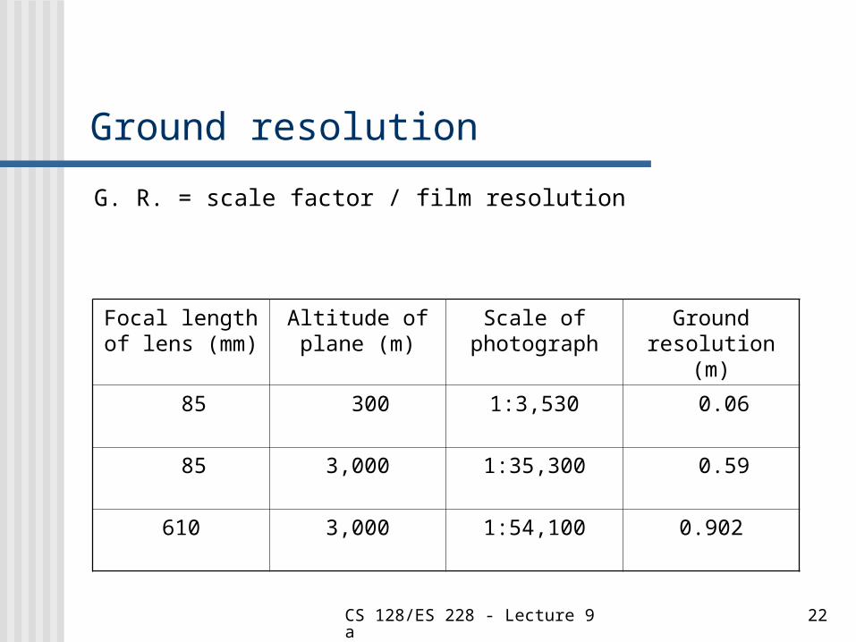
Ground resolution

G. R. = scale factor / film resolution

Focal length of lens (mm)

Altitude of plane (m)

Scale of photograph

Ground resolution (m)

85 300 1:3,530 0.06

85 3,000 1:35,300 0.59

610 3,000 1:54,100 0.902


Spatial resolution: digital (satellite) images

A sampler of recent (civilian) satellites:Sponsor Satellite (instrument) Year Res. (m)

NASA Landsat (Thematic Mapper) 1980-90s 30 (MSS)

NASA & others

EOS Terra (ASTER) 2000 15 - 90 (MSS)

France SPOT-3 to 5 1993-2002

10 to 5 (pan)

Space Imaging

IKONOS-2 1999 1 (pan)4 (MSS)

EarthWatch Quickbird-2 2001 0.6 (pan)2.5 (MSS)


Satellite image resolution

Quickbird 2 Commercial venture

0.63 m resolution

U.S. trying to discourage open access to finer resolution images

Digitalglobe.com


Satellite orbits

Geostationary 36,000 km above

equator

Polar varying heights

often in Sun-synchronous orbits

Both diagrams from European Organisation for the Exploitation of Meteorological Satelliteswww.eumetsat.de/en/mtp/space/polar.html


Satellite coverage

Geostationary no polar coverage coverage is 24/7 low ground reso-lution

(~ 1 km)

Polar global coverage coverage is dis-

continuous

Both diagrams from European Organisation for the Exploitation of Meteorological Satelliteswww.eumetsat.de/en/mtp/space/polar.html


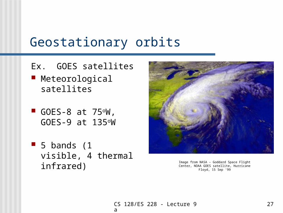
Geostationary orbits

Ex. GOES satellites Meteorological

satellites

GOES-8 at 75oW, GOES-9 at 135oW

5 bands (1 visible, 4 thermal infrared) Image from NASA – Goddard Space Flight

Center, NOAA GOES satellite, Hurricane Floyd, 15 Sep ‘99


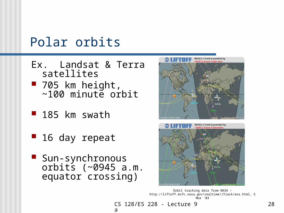
Polar orbits

Ex. Landsat & Terra satellites

705 km height, ~100 minute orbit

185 km swath

16 day repeat

Sun-synchronousorbits (~0945 a.m. equator crossing)

Orbit tracking data from NASA – http://liftoff.msfc.nasa.gov/realtime/JTrack/eos.html, 5 Mar ‘03

cs 128/es 228 - lecture 9a1 principles of remote sensing image from nasa – goddard space flight...

Documents