crust to core workshop: an introduction to perple_x
DESCRIPTION
Crust to Core workshop: An introduction to Perple_X. Part 2: The structure of a Perple_X calculation. Perple_X: Is written and maintained by Jamie Connolly (ETH Z ürich) Is written in FORTRAN, with the source code available. Took quite a long time to write… - PowerPoint PPT PresentationTRANSCRIPT
Crust to Core workshop:An introduction to Perple_X
Part 2: The structure of a Perple_X calculation
Institute of Mineralogy and Petrology

Perple_X:
• Is written and maintained by Jamie Connolly (ETH Zürich)
• Is written in FORTRAN, with the source code available.
• Took quite a long time to write…
• Accepts thermodynamic data from any source, provided it is formatted correctly (in a simple text file).
Connolly, J.A.D., Kerrick, D.M., 1987. An algorithm and computer program for calculating composition phase diagrams. Computers and Geosciences 11, 1-55.
Connolly, J.A.D., 1990. Multivariable phase diagrams: an algorithm based on generalized thermodynamics. Am. J. Sci. 290, 666-718.
Kerrick, D.M., Connolly, J.A.D., 2001. Metamorphic devolatilization of subducted marine sediments and the transport of volatiles into the Earth's mantle. Nature 411, 293-296.
Connolly, J.A.D., Petrini, K., 2002. An automated strategy for calculation of phase diagram sections and retrieval of rock properties as a function of physical conditions. J. Metamorph. Geol. 20, 697-708.
Connolly, J.A.D., 2005. Computation of phase equilibria by linear programming: A tool for geodynamic modeling and its application to subduction zone decarbonation. Earth Planet. Sci. Lett. 236, 524-541.
Caddick, M.J., Thompson, A.B., 2008. Quantifying the tectono-metamorphic evolution of pelitic rocks from a wide range of tectonic settings: Mineral compositions in equilibrium. Contrib. Mineral. Petrol. 156, 177-195.

Perple_X:
• Minimises free energy of multiple phase configurations to identify the ‘most stable’ set.
• Can work with complex phases by breaking solution-space into a number of discrete ‘phases’ (pseudo-compounds).
• Is very flexible, generating:
• PT projections
• Pseudosections
• Compatability diagrams (e.g. AFM triangles)
• Mixed-variable diagrams
• Is very flexible, allowing:
• Complex saturation heirarchies
• Transformation of components
• Use of numerous EOS for fluids involving H2O, CO2, NaCl
• Easy extraction of sub-systems from large solution model files
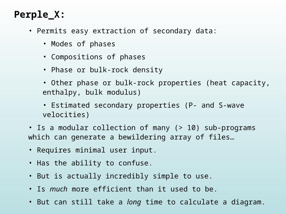
Perple_X:
• Permits easy extraction of secondary data:
• Modes of phases
• Compositions of phases
• Phase or bulk-rock density
• Other phase or bulk-rock properties (heat capacity, enthalpy, bulk modulus)
• Estimated secondary properties (P- and S-wave velocities)
• Is a modular collection of many (> 10) sub-programs which can generate a bewildering array of files…
• Requires minimal user input.
• Has the ability to confuse.
• But is actually incredibly simple to use.
• Is much more efficient than it used to be.
• But can still take a long time to calculate a diagram.

Build(Problem setup)
Pssect(Postscript plot generator)
Werami(Secondary data
extraction)
Vertex(Free energy minimisation)
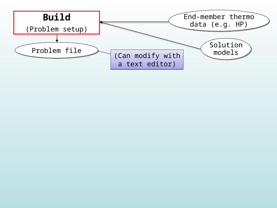
Problem fileProblem file
Build(Problem setup)
(Can modify with a text editor)
(Can modify with a text editor)
Solution models
Solution models
End-member thermo data (e.g. HP)
End-member thermo data (e.g. HP)
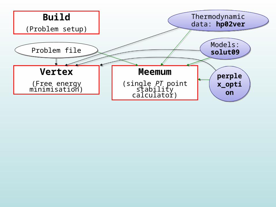
Meemum(single PT point stability
calculator)
Vertex(Free energy minimisation)
Build(Problem setup)
Solution models
Solution modelsProblem fileProblem file
End-member thermo data (e.g. HP)
End-member thermo data (e.g. HP)
Other optionsOther
options
Models: solut09Models: solut09
Thermodynamic data: hp02ver
Thermodynamic data: hp02ver
perplex_option
perplex_option
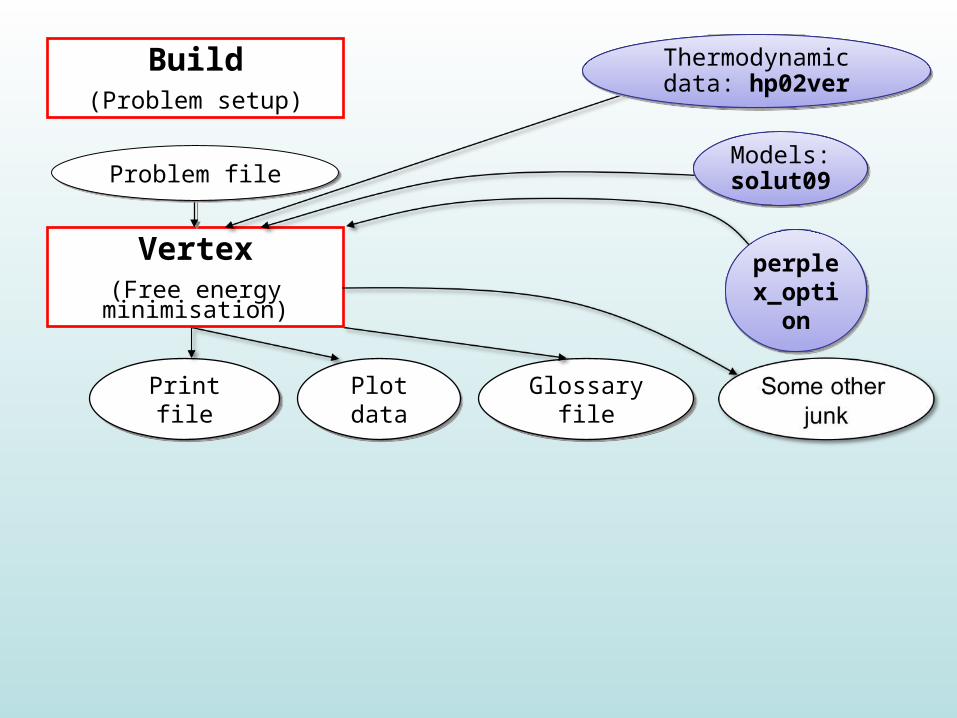
Print filePrint file Plot dataPlot data Glossary fileGlossary file
Vertex(Free energy minimisation)
Build(Problem setup)
Solution models
Solution modelsProblem fileProblem file
End-member thermo data (e.g. HP)
End-member thermo data (e.g. HP)
Other optionsOther
options
Models: solut09Models: solut09
Thermodynamic data: hp02ver
Thermodynamic data: hp02ver
perplex_option
perplex_option

Some other junk
Some other junk
Build(Problem setup)
Pssect(Postscript generator)
Illustrator/Coreldraw/etc(Making it look good…)
.ps file.ps file
Glossary fileGlossary file
Vertex(Free energy minimisation)
Solution models
Solution modelsProblem fileProblem file
End-member thermo data (e.g. HP)
End-member thermo data (e.g. HP)
Other optionsOther
options
Plot dataPlot dataPrint filePrint file

data filedata file
Werami(Extra data extraction)
Build(Problem setup)
Pssect(Postscript generator)
.ps file.ps file
Illustrator/Coreldraw/etc(Making it look good…)
Matlab (pscontor)Contouring routine
Vertex(Free energy minimisation)
Some other junk
Some other junk
Glossary fileGlossary file
Solution models
Solution modelsProblem fileProblem file
End-member thermo data (e.g. HP)
End-member thermo data (e.g. HP)
Plot dataPlot dataPrint filePrint file
Other optionsOther
options

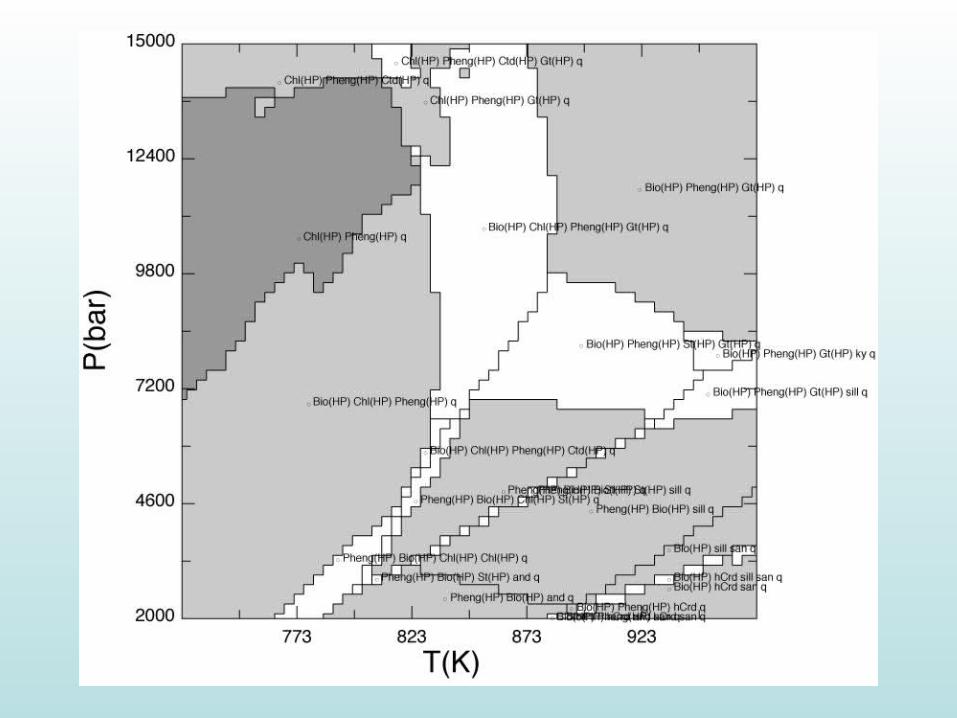
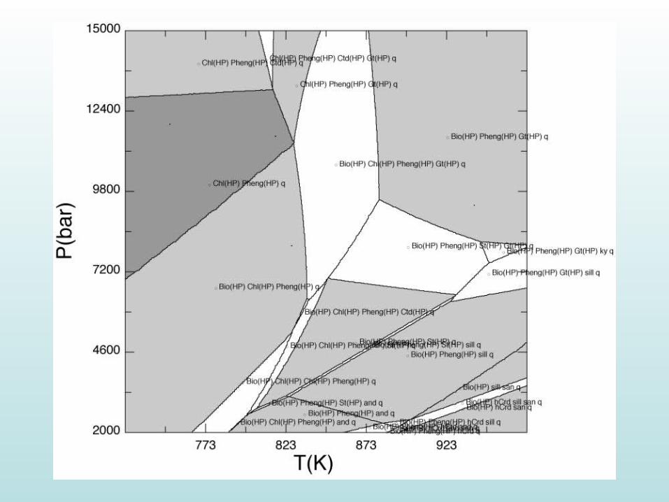
Exercise 1:
Use build, vertex and pssect to produce a phase-stability map (pseudosection) for a simplified pelitic rock composition (in molar proportions: 3.82 % K2O, 10.53 % FeO, 4.76 % MgO, 12.49 % Al2O3, 68.00 % SiO2 + H2O) at 2 - 15 kbars, 450 - 700 ˚C.


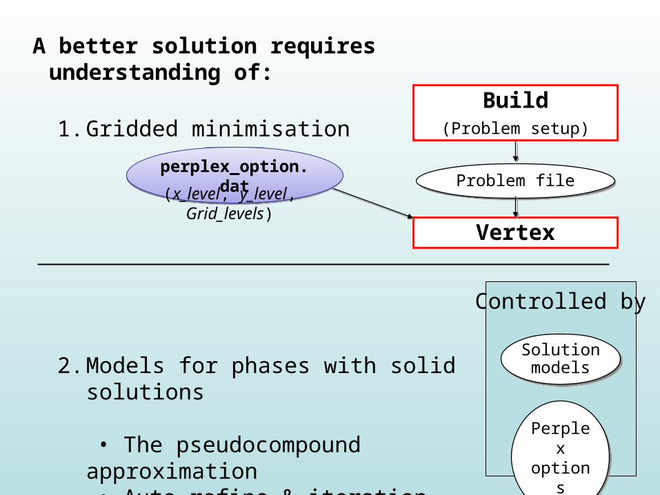
A better solution requires understanding of:
1. Gridded minimisation
2. Models for phases with solid solutions • The pseudocompound approximation • Auto refine & iteration
Problem fileProblem file
Solution models
Solution models
Perplex optionsPerplex options
Controlled by
Vertex
perplex_option.datperplex_option.dat
Build(Problem setup)
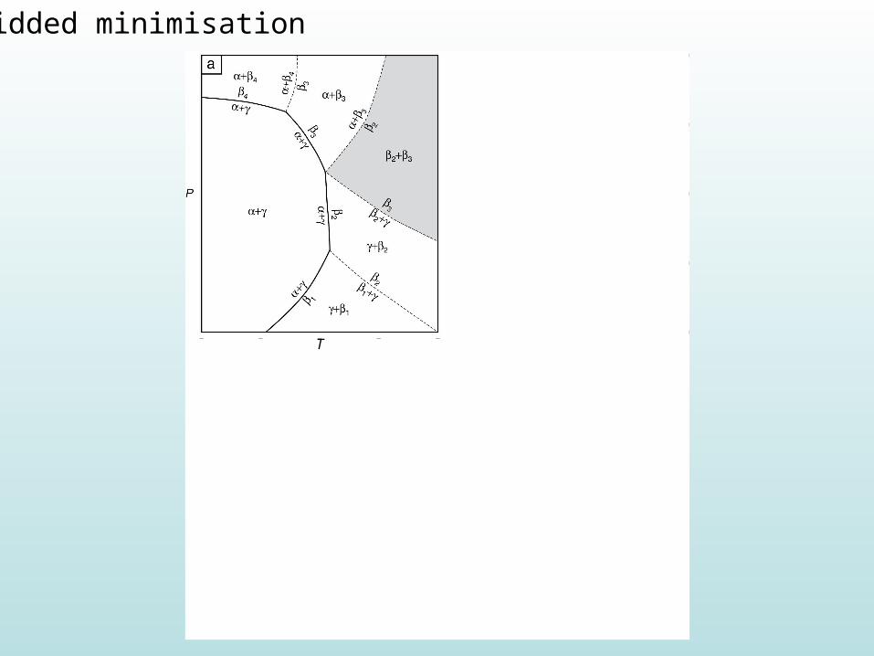
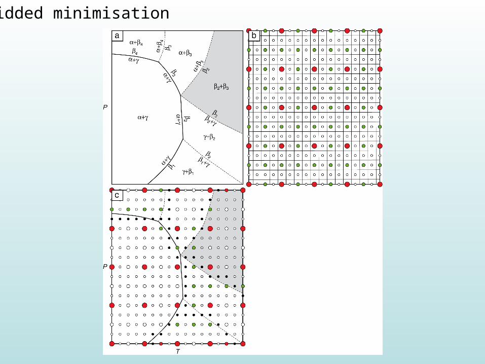
Gridded minimisation
T

Gridded minimisation
T

Gridded minimisation
Gridded minimisation

Gridded minimisation
In the “perplex_options.dat” file:
• x_nodes & y_nodes define the number of red dots
• grid_levels defines the amount of iteration
y_no
des
= 5
x_nodes = 5
Grid_levels = 3 (red, green &
black)
A better solution requires understanding of:
1. Gridded minimisation
2. Models for phases with solid solutions • The pseudocompound approximation • Auto refine & iteration
Problem fileProblem file
Solution models
Solution models
Perplex optionsPerplex options
Controlled by
Vertex
perplex_option.datperplex_option.dat
Build(Problem setup)
(x_level, y_level,Grid_levels)
Solution model intro
Solution models for complex phases

Solution model intro
Solution models for complex phases
Phases of variable composition, (solution phases), are invariably described as a mixture of s real or hypothetical endmembers, for which data is tabulated. The problem is then to formulate a solution model that describes the Gibbs energy of such a solution phase in terms of these endmembers. Such models consist of three components G = Gmech + Gconf + Gexcess where Gmech is the energy arising from mechanically mixing of the endmembers, Gconf is the energy expected to arise from theoretical entropic considerations, and Gexcess is a component that accounts for the energetic effects caused by distortions of the atomic structure (e.g., strain) of the chemical mixing process or, in some cases, simply error in Gconf.
(Connolly, 2006)

Solution model intro
Three main types of solution model:
• Ideal (∆Sconfig considered, ∆Gexcess not considered)• Regular (∆Sconfig & ∆Gexcess considered)• Asymmetric (as above, minima not at Xi = 0.5)
Three levels of complexity:
• Single site mixing (e.g. Mg Fe in olivine; Mg, Fe, Ca, Mn mixing in garnet)• Multiple site mixing (e.g. Mg, Fe, Ca, Mn & Fe3+ Al in garnet)• Multiple site mixing requiring charge balance (e.g.
NaSi CaAl in plagioclase feldspar)
É
É
É

entropy
Assuming simple binary mixing e.g. Fe-Mg in garnet
In a simple mechanical mixture, energy varies linearly between the values of the two end-members
In an ideal solid solution, configurational entropy must be considered

Entropy2
Assuming simple binary mixing e.g. Fe-Mg in garnet
Configurational entropy is a function of disorder, so logically must be at a maximum when the Xi = 0.5. It follows that Sconfig must always be positive.
Entropy
-15
-10
-5
0
5
10
15
0 0.1 0.2 0.3 0.4 0.5 0.6 0.7 0.8 0.9 1
Mole fraction, Xi
Enthalpy & Gibbs Energy: J/mol.
Entropy: J/mol/K
Entropy
Entropy2
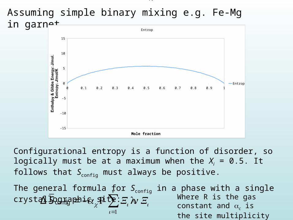
Assuming simple binary mixing e.g. Fe-Mg in garnet
Configurational entropy is a function of disorder, so logically must be at a maximum when the Xi = 0.5. It follows that Sconfig must always be positive.
The general formula for Sconfig in a phase with a single crystallographic site:
Entropy
-15
-10
-5
0
5
10
15
0 0.1 0.2 0.3 0.4 0.5 0.6 0.7 0.8 0.9 1
Mole fraction, Xi
Enthalpy & Gibbs Energy: J/mol.
Entropy: J/mol/K
Entropy
∆ Sconfig =−αc R Xi lnXii=1
n
∑ Where R is the gas constant and αc is the site multiplicity

Entropy2
Assuming simple binary mixing e.g. Fe-Mg in garnet
In our binary case:
∆ SConfig =−αc R Xi lnXi + 1−Xi[ ] ln 1−Xi[ ]( )
Where R is the gas constant and αc is the site multiplicity
∆ SConfig =−αc R XA lnXA + XB lnXB( )
Entropy
-15
-10
-5
0
5
10
15
0 0.1 0.2 0.3 0.4 0.5 0.6 0.7 0.8 0.9 1
Mole fraction, Xi
Enthalpy & Gibbs Energy: J/mol.
Entropy: J/mol/K
Entropy
Entropy
-15
-10
-5
0
5
10
15
0 0.1 0.2 0.3 0.4 0.5 0.6 0.7 0.8 0.9 1
Mole fraction, Xi
Enthalpy & Gibbs Energy: J/mol.
Entropy: J/mol/K
Entropy
Entropy2
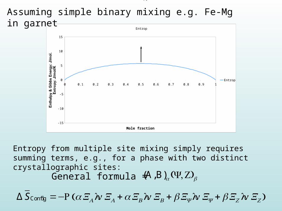
Assuming simple binary mixing e.g. Fe-Mg in garnet
Entropy from multiple site mixing simply requires summing terms, e.g., for a phase with two distinct crystallographic sites:
∆ SConfig =−R αXA lnXA +αXB lnXB + βXY lnXY + βXZ lnXZ( )
(A,B)α (Y ,Z)βGeneral formula =
Solution model intro
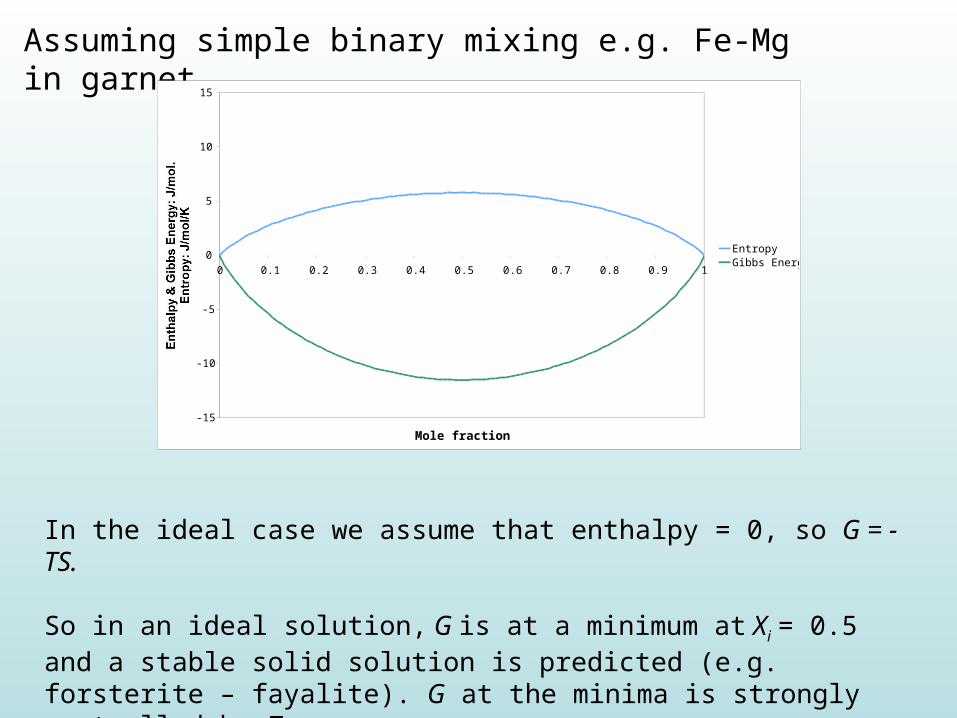
Assuming simple binary mixing e.g. Fe-Mg in garnet
In the ideal case we assume that enthalpy = 0, so G = -TS.
So in an ideal solution, G is at a minimum at Xi = 0.5 and a stable solid solution is predicted (e.g. forsterite – fayalite). G at the minima is strongly controlled by T.
-15
-10
-5
0
5
10
15
0 0.1 0.2 0.3 0.4 0.5 0.6 0.7 0.8 0.9 1
Mole fraction, Xi
Enthalpy & Gibbs Energy: J/mol.
Entropy: J/mol/K
EntropyGibbs Energy
Solution model intro
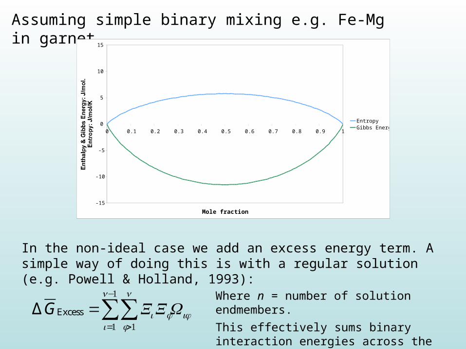
Assuming simple binary mixing e.g. Fe-Mg in garnet
In the non-ideal case we add an excess energy term. A simple way of doing this is with a regular solution (e.g. Powell & Holland, 1993):
∆GExcess = XiXjWijj>1
n
∑i=1
n−1
∑Where n = number of solution endmembers.
This effectively sums binary interaction energies across the entire phase
-15
-10
-5
0
5
10
15
0 0.1 0.2 0.3 0.4 0.5 0.6 0.7 0.8 0.9 1
Mole fraction, Xi
Enthalpy & Gibbs Energy: J/mol.
Entropy: J/mol/K
EntropyGibbs Energy

Solution model intro
Assuming simple binary mixing e.g. Fe-Mg in garnet
In our Mg–Fe binary, this simplifies to:
∆GExcess =XFeXMgWFe-Mg
Where WFe-Mg is typically an empirically-defined energy (J mol-1) which can be positive or negative, and can be P or T dependent.
-15
-10
-5
0
5
10
15
0 0.1 0.2 0.3 0.4 0.5 0.6 0.7 0.8 0.9 1
Mole fraction, Xi
Enthalpy & Gibbs Energy: J/mol.
Entropy: J/mol/K
EntropyGibbs Energy

Solution model intro
Assuming simple binary mixing e.g. Fe-Mg in garnet
Total molar Gibbs energy is now a function of both entropy and excess terms (G = H -TS)
-15
-10
-5
0
5
10
15
0 0.1 0.2 0.3 0.4 0.5 0.6 0.7 0.8 0.9 1
Mole fraction, Xi
Enthalpy & Gibbs Energy: J/mol.
Entropy: J/mol/K
EntropyEnthalpyGibbs Energy

Solution model intro
Assuming simple binary mixing e.g. Fe-Mg in garnet
If the Wij term (the Margules parameter) is strongly positive, the resultant G curve can develop two minima - a solvus is predicted.
Since the entropy term dominates at high T, solvii are predicted at low temperatures.
-15
-10
-5
0
5
10
15
0 0.1 0.2 0.3 0.4 0.5 0.6 0.7 0.8 0.9 1
Mole fraction, Xi
Enthalpy & Gibbs Energy: J/mol.
Entropy: J/mol/K
EntropyEnthalpyGibbs Energy
Solution model intro
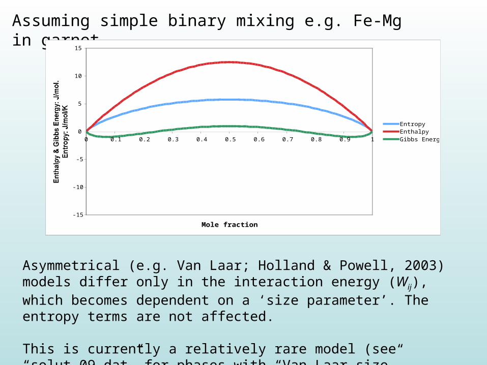
Assuming simple binary mixing e.g. Fe-Mg in garnet
Asymmetrical (e.g. Van Laar; Holland & Powell, 2003) models differ only in the interaction energy (Wij), which becomes dependent on a ‘size parameter’. The entropy terms are not affected.
This is currently a relatively rare model (see “solut_09.dat” for phases with “Van Laar size” definitions)
-15
-10
-5
0
5
10
15
0 0.1 0.2 0.3 0.4 0.5 0.6 0.7 0.8 0.9 1
Mole fraction, Xi
Enthalpy & Gibbs Energy: J/mol.
Entropy: J/mol/K
EntropyEnthalpyGibbs Energy
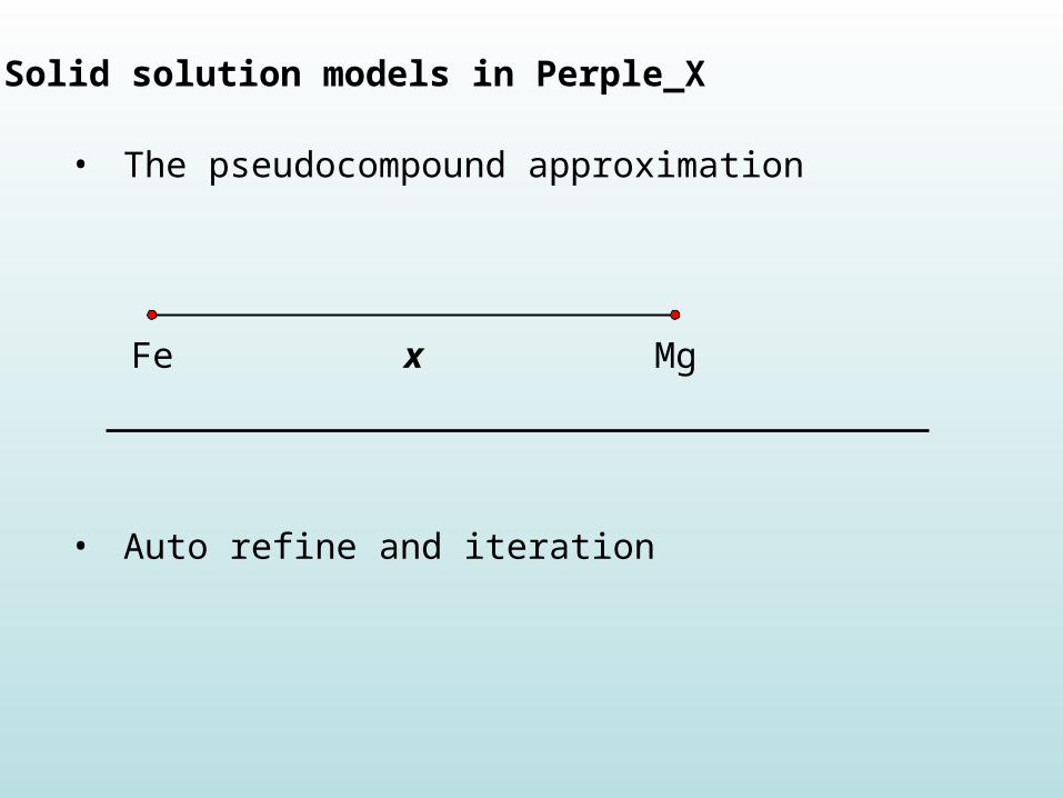
Solid solution models in Perple_X
• The pseudocompound approximation
• Auto refine and iteration
Solid solution models in Perple_X
• The pseudocompound approximation
• Auto refine and iteration
Fe Mgx

Fe Mg
Solid solution models in Perple_X
• The pseudocompound approximation
• Auto refine and iteration

Solid solution models in Perple_X
• The pseudocompound approximation
• Auto refine and iteration
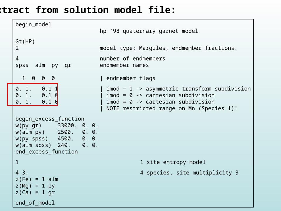
begin_model hp '98 quaternary garnet model
Gt(HP) 2 model type: Margules, endmember fractions.
4 number of endmembers spss alm py gr endmember names
1 0 0 0 | endmember flags
0. 1. 0.1 1 | imod = 1 -> asymmetric transform subdivision0. 1. 0.1 0 | imod = 0 -> cartesian subdivision0. 1. 0.1 0 | imod = 0 -> cartesian subdivision
| NOTE restricted range on Mn (Species 1)!
begin_excess_functionw(py gr) 33000. 0. 0. w(alm py) 2500. 0. 0.w(py spss) 4500. 0. 0. w(alm spss) 240. 0. 0.end_excess_function
1 1 site entropy model
4 3. 4 species, site multiplicity 3z(Fe) = 1 almz(Mg) = 1 pyz(Ca) = 1 gr
end_of_model
Extract from solution model file:
0. 1. 0.1 10. 1. 0.1 00. 1. 0.1 0
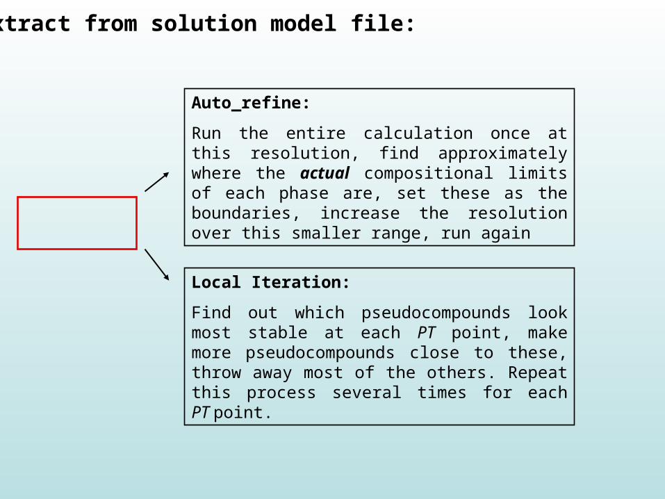
Extract from solution model file:
Auto_refine:
Run the entire calculation once at this resolution, find approximately where the actual compositional limits of each phase are, set these as the boundaries, increase the resolution over this smaller range, run again
Local Iteration:
Find out which pseudocompounds look most stable at each PT point, make more pseudocompounds close to these, throw away most of the others. Repeat this process several times for each PT point.
0. 1. 0.1 10. 1. 0.1 00. 1. 0.1 0
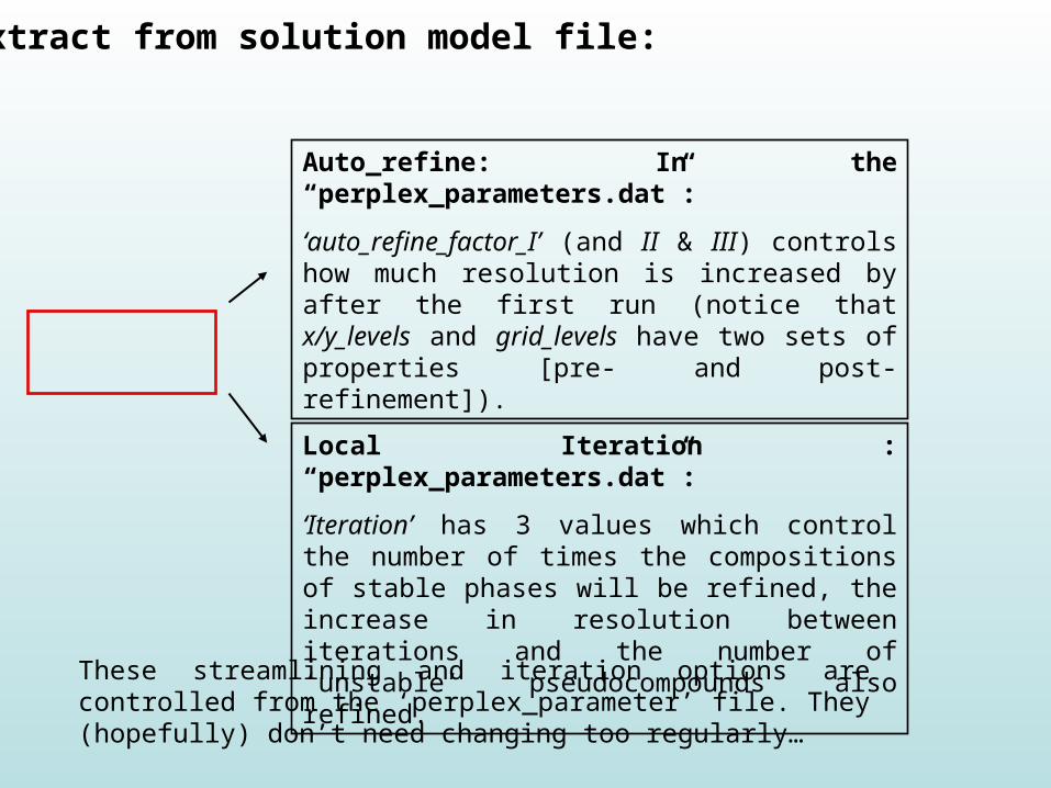
Extract from solution model file:
Auto_refine: In the “perplex_parameters.dat”:
‘auto_refine_factor_I’ (and II & III) controls how much resolution is increased by after the first run (notice that x/y_levels and grid_levels have two sets of properties [pre- and post-refinement]).
Local Iteration : “perplex_parameters.dat”:
‘Iteration’ has 3 values which control the number of times the compositions of stable phases will be refined, the increase in resolution between iterations and the number of ‘unstable’ pseudocompounds also refined.
These streamlining and iteration options are controlled from the ‘perplex_parameter’ file. They (hopefully) don’t need changing too regularly…
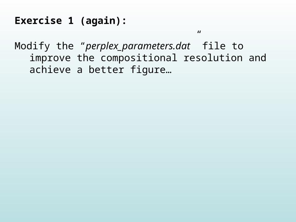
Exercise 1 (again):
Modify the “perplex_parameters.dat” file to improve the compositional resolution and achieve a better figure…


Solution model intro
Further reading:
Derivation of configurational entropy terms:
• Jamie Connolly’s course notes (lecture 6)
• Spear, 1993, Metamorphic phase equilibria and P-T-t paths, first few pages of chapter 7.
Regular solution models:
• Powell & Holland, 1993, American Mineralogist, v78, 1174-1180.
Van Laar solution models:
• Holland & Powell, 2003, Contributions to Mineralogy & Petrology, v145, 492-501.
Entropy2
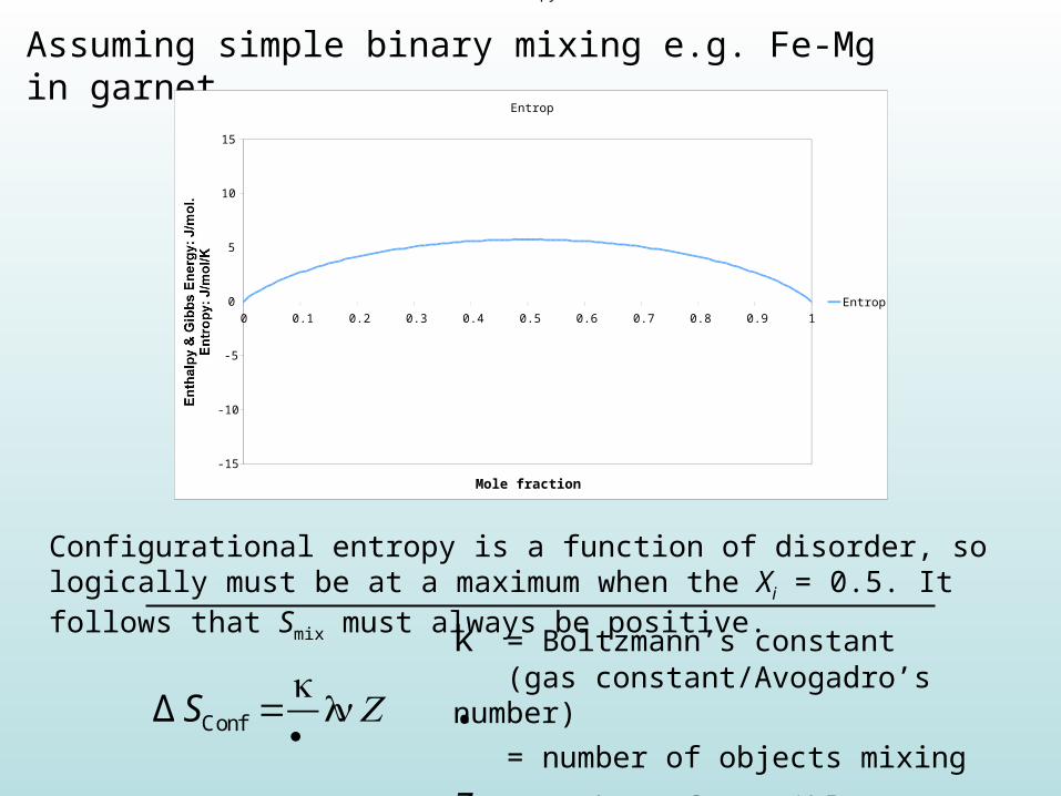
Assuming simple binary mixing e.g. Fe-Mg in garnet
Configurational entropy is a function of disorder, so logically must be at a maximum when the Xi = 0.5. It follows that Smix must always be positive.
Entropy
-15
-10
-5
0
5
10
15
0 0.1 0.2 0.3 0.4 0.5 0.6 0.7 0.8 0.9 1
Mole fraction, Xi
Enthalpy & Gibbs Energy: J/mol.
Entropy: J/mol/K
Entropy
∆ SConf =
k•
lnZ
k = Boltzmann’s constant(gas constant/Avogadro’s number)
= number of objects mixing
Z = number of possible configurations •

Entropy2
Assuming simple binary mixing e.g. Fe-Mg in garnet
Configurational entropy is a function of disorder, so logically must be at a maximum when the Xi = 0.5. It follows that Smix must always be positive.
Entropy
-15
-10
-5
0
5
10
15
0 0.1 0.2 0.3 0.4 0.5 0.6 0.7 0.8 0.9 1
Mole fraction, Xi
Enthalpy & Gibbs Energy: J/mol.
Entropy: J/mol/K
Entropy
∆ SConf =
k•
lnZ Z =
•• !
For single kindof mixing object,