crr 294 090423-final reports/cooperative research... · rapport des recherches collectives ... 5.6...
TRANSCRIPT

ICES COOPERATIVE RESEARCH REPORT Rapport des Recherches Collectives
NO. 295
MAY 2009
Manual of recommended practices
for modelling physical – biological interactions
during fish early life
Editors
Elizabeth W. North • Alejandro Gallego • Pierre Petitgas
Authors
Bjørn Ådlandsvik • Joachim Bartsch • David Brickman
Howard I. Browman • Karen Edwards • Øyvind Fiksen
Alejandro Gallego • Albert J. Hermann • Sarah Hinckley
Edward Houde • Martin Huret • Jean-Olivier Irisson
Geneviève Lacroix • Jeffrey M. Leis • Paul McCloghrie
Bernard A. Megrey • Thomas Miller • Johan van der Molen
Christian Mullon • Elizabeth W. North • Carolina Parada
Claire B. Paris • Pierre Pepin • Pierre Petitgas
Kenneth Rose • Uffe H. Thygesen • Cisco Werner

International Council for the Exploration of the Sea Conseil International pour l’Exploration de la Mer
H. C. Andersens Boulevard 44 – 46 DK‐1553 Copenhagen V Denmark Telephone (+45) 33 38 67 00 Telefax (+45) 33 93 42 15 www.ices.dk [email protected]
Recommended format for purposes of citation: North, E. W., Gallego, A., Petitgas, P. (Eds). 2009. Manual of recommended practices for modelling physical – biological interactions during fish early life. ICES Coopera‐tive Research Report No. 295. 111 pp.
When citing specific chapters, it is recommended that authors be given due credit in the following form of reference. Houde, E. D., and Bartsch, J. 2009. Mortality. In Manual of Recommended Practices for Modelling Physical – Biological Interactions during Fish Early Life, pp. 27 – 42. Ed. by E. W. North, A. Gallego, and P. Petitgas. ICES Cooperative Research Report No. 295. 111 pp.
For permission to reproduce material from this publication, please apply to the Gen‐eral Secretary.
This document is a report of an expert group under the auspices of the International Council for the Exploration of the Sea and does not necessarily represent the view of the Council.
ISBN 978 – 87 – 7482 – 060 – 4
ISSN 1017 – 6195
© 2009 International Council for the Exploration of the Sea

ICES Cooperative Research Report No. 295 | i
Contents
Foreword ..................................................................................................................................1
Executive summary ................................................................................................................2
1 Hydrodynamic models .................................................................................................3 1.1 Hydrodynamic model components ...................................................................3
1.1.1 Horizontal discretization ........................................................................3 1.1.2 Vertical discretization..............................................................................4 1.1.3 Time evolution .........................................................................................5 1.1.4 Using hydrodynamic output for particle tracking ..............................5
1.2 Characteristics of an appropriate hydrodynamic model ................................6 1.2.1 Boundaries and initial conditions..........................................................7 1.2.2 Resolution .................................................................................................7 1.2.3 Model validation......................................................................................8 1.2.4 Small‐scale physics ..................................................................................8
2 Particle tracking .............................................................................................................9 2.1 Best practices for particle tracking .....................................................................9
2.1.1 Choice of model .......................................................................................9 2.1.2 Time discretization ................................................................................10 2.1.3 Choice of time‐step ................................................................................10 2.1.4 Number of particles...............................................................................11 2.1.5 Choice of random number generator..................................................11 2.1.6 Boundary conditions .............................................................................12 2.1.7 Additional considerations ....................................................................12
2.2 Test cases..............................................................................................................14 2.2.1 Vertical distribution of buoyant particles...........................................14 2.2.2 Flow around an obstacle .......................................................................16
3 Biological processes ....................................................................................................20 3.1 Initial conditions: spawning locations .............................................................20
3.1.1 Egg‐production models ........................................................................21 3.2 Pelagic larval duration .......................................................................................23 3.3 Growth .................................................................................................................25 3.4 Mortality ..............................................................................................................27
3.4.1 Introduction............................................................................................27 3.4.2 Larval mortality: concepts and relationships.....................................30 3.4.3 Causes of early‐life mortality ...............................................................35 3.4.4 Case study: mortality and the super‐individual concept .................38
3.5 Behaviour and settlement..................................................................................42 3.5.1 Introduction............................................................................................42 3.5.2 General questions on behaviour‐related traits...................................43 3.5.3 Vertical position .....................................................................................45 3.5.4 Horizontal swimming ...........................................................................48

ii | Modelling physical–biological interactions during fish early life
3.5.5 Orientation..............................................................................................51 3.5.6 Foraging ..................................................................................................53 3.5.7 Predator avoidance................................................................................55 3.5.8 Schooling.................................................................................................55 3.5.9 Choice of settlement ..............................................................................57
4 Application 1: adaptive sampling.............................................................................60 4.1 Key considerations and processes ....................................................................60 4.2 Best practices .......................................................................................................61 4.3 Research needs ....................................................................................................62 4.4 Final recommendations......................................................................................62
5 Application 2: connectivity ........................................................................................63 5.1 Definition of connectivity and scope of connectivity models.......................63 5.2 Decide which questions the model should answer........................................64 5.3 Identify the scale of the connectivity model ...................................................64
5.3.1 Spatial scales...........................................................................................64 5.3.2 Temporal scales......................................................................................65
5.4 Gain knowledge of processes relevant to modelling connectivity ..............65 5.4.1 Initial conditions: spawning time and locations................................65 5.4.2 Suitable settlement locations ................................................................65 5.4.3 Small‐scale physics: turbulence ...........................................................66 5.4.4 Large‐scale physics: grid size and domain.........................................67
5.5 Lagrangian parameterization and online – offline methods..........................68 5.5.1 Parameterization of the Lagrangian statistics....................................68 5.5.2 Online – offline methods........................................................................68
5.6 Larval stage duration .........................................................................................69 5.7 Larval traits: growth and mortality..................................................................69 5.8 Larval traits: larval behaviour...........................................................................70 5.9 Steps towards the state‐of‐the‐art model.........................................................70
5.9.1 Step 1: minimum model........................................................................70 5.9.2 Step 2: biological features .....................................................................71 5.9.3 Step 3: small‐scale features ...................................................................71
5.10 Result analysis and model validation ..............................................................71 5.10.1 Dispersal kernel .....................................................................................71 5.10.2 Transition probability matrix ...............................................................72
5.11 Model validation.................................................................................................73 5.11.1 Trajectory path .......................................................................................74 5.11.2 Population connectivity results ...........................................................75
5.12 Research needs ....................................................................................................75 5.12.1 Initial dispersal.......................................................................................75 5.12.2 Settlement ...............................................................................................75

ICES Cooperative Research Report No. 295 | iii
6 Application 3: recruitment prediction .....................................................................77 6.1 Definition .............................................................................................................77 6.2 Objectives of recruitment prediction................................................................77 6.3 Indices of recruitment from ICPBMs ...............................................................78 6.4 The need for a conceptual model......................................................................78 6.5 Forecasting accuracy ..........................................................................................80 6.6 Techniques for forecasting ................................................................................80 6.7 Philosophy of modelling....................................................................................81
7 Looking to the future: recommendations and research needs.............................83
Acknowledgements .............................................................................................................86
8 References .....................................................................................................................87
Annex 1: Particle tracking: Euler vs. Runge – Kutta stepping schemes..................102
Annex 2: Particle tracking: the effect of time‐steps...................................................103
Annex 3: NPZ parameters, functions, and data assimilation...................................105
Annex 4: Coupling NPZ to physical models: types of coupling, scaling, and resolution..................................................................................................106
Annex 5: Coupling NPZ and particle‐tracking models: patchiness, trophic feedback, and behavioural responses.........................................................107
Author contact information..............................................................................................108
Acronyms and abbreviations ...........................................................................................111


ICES Cooperative Research Report No. 295 | 1
Foreword
This manual of recommended practices is a product of the “Workshop on Advance‐ments in Modelling Physical – Biological Interactions in Fish Early Life History: Rec‐ommended Practices and Future Directions” (WKAMF; http://northweb.hpl. umces.edu/research/wkamf_intro.htm). The WKAMF was held 3 – 5 April 2006 in Nantes, France. The goal was to evaluate the current state and next steps in the de‐veloping field of modelling physical – biological interactions in the early life of fish. The workshop focused on recent advances in coupled biological – physical models that incorporate predictions from three‐dimensional circulation models to determine the transit of fish eggs, larvae, and juveniles from spawning to nursery areas. These coupled biophysical models provide new insight into how planktonic dispersal, growth, and survival are mediated by physical and biological conditions, and how they have contributed to enhanced understanding of fish population variability and stock structure.
The workshop was designed to survey major components of bio‐physical models of fish early life, address numerical techniques and validation issues, define recom‐mended modelling practices, and identify future research needs. Sev‐eral aspects of modelling fish early life history were addressed, includ‐ing: initial conditions (egg produc‐tion, spawning location/time), small‐scale processes (turbulence, feeding success), mesoscale transport processes (physics and larval behaviour), and biological processes (development, growth, mortality, juvenile recruitment, meta‐morphosis, settlement). Workshop participants agreed on six major themes that rep‐resented important research needs in modelling physical – biological interactions and would result in advances in the field: validation and sensitivity methods, model complexity, mortality, behaviour and cues, energetics, and physics.
Papers based on some of the research presented at WKAMF appeared in a theme sec‐tion in the Marine Ecology Progress Series entitled “Advances in modelling physical – biological interactions in fish early life history”. These open‐access publications can be found at http://www.int‐res.com/abstracts/meps/v347/.
WKAMF was attended by 54 participants from 14 countries and was chaired by Ale‐jandro Gallego (UK), Elizabeth North (USA), and Pierre Petitgas (France). WKAMF was held under the auspices of the ICES Working Group on Physical – Biological In‐teractions and the ICES Working Group on Recruitment Processes. It was hosted by the French Research Institute for Exploitation of the Sea (IFREMER) with support from IFREMER, US National Science Foundation (NSF), US National Marine Fisher‐ies Service (NMFS), UK Fisheries Research Services (FRS), and the University of Maryland Center for Environmental Science (UMCES). It was endorsed by Global Ocean Ecosystems Dynamics (GLOBEC) and Eur‐Oceans.
WKAMF logo.

2 | Modelling physical–biological interactions during fish early life
Executive summary
The objectives of this manual of recommended practices (MRP) are to summarize appropriate methods for modelling physical – biological interactions during the early life of fish, to recommend modelling techniques in the context of specific applica‐tions, and to identify gaps in knowledge. This manual is intended to provide a refer‐ence for early‐career modellers who are interested in applying numerical models to fish early life and who would benefit from a summary of recommended practices for coupled biological – physical models that incorporate predictions from three‐dimensional circulation models to determine the transit of fish eggs, larvae, and ju‐veniles from spawning to nursery areas. For current practitioners of numerical mod‐elling in fish early life, the manual provides updates on latest techniques and areas in need of further research. Although the manual focuses on finfish, many of the sum‐marized modelling techniques and recommended practices apply to modelling planktonic organisms, including zooplankton and other meroplankton (e.g. molluscs and crustaceans).
It is important to recognize that “best” modelling practices depend upon the objective of the modelling exercise. In other words, no single model is appropriate to all appli‐cations. Instead, model formulations are situation‐specific. Because methodologies depend upon the goal of the endeavour, this manual includes an overview of basic components of fish early life models and presents recommendations in the context of three specific applications: adaptive sampling, connectivity, and recruitment predic‐tion.
The first three sections (Section 1 – Hydrodynamic models, Section 2 – Particle track‐ing, and Section 3 – Biological processes) summarize methodologies that are impor‐tant components of three‐dimensional models of the early life of fish. The next three sections (Section 4 – Application 1: adaptive sampling, Section 5 – Application 2: con‐nectivity, and Section 6 – Application 3: recruitment prediction) discuss the applica‐tion of selected methodologies to specific issues that are commonly addressed with these models. The final section summarizes the information gaps and research needs identified throughout the manual.
This MRP grew out of participant discussions at the “Workshop on Advancements in Modelling Physical – Biological Interactions in Fish Early Life History: Recommended Practices and Future Directions” (WKAMF) held on 3 – 5 April 2006 in Nantes, France. This manual does not contain an exhaustive review of all approaches to modelling the early life of fish. Instead, it is intended to be a general reference for fish early life modelling that includes citations that will direct readers to in‐depth treatments of specific topics. In addition, it should be noted that this document does not represent the consensus recommendations of all authors. Each section was written separately. In some cases, differences in recommendations and perspectives exist. These appar‐ent contradictions may stem from dissimilarity in the time or space scale of the mod‐els used by the authors or the ecosystem in which the authors are most experienced (e.g. temperate vs. tropical). The issues on which recommendations or perspective diverge are those that remain an active area of research. This manual is a “living” document: future revisions and updates are expected as our understanding and methods evolve.
ICES Cooperative Research Report No. 295 | 3
1 Hydrodynamic models
Genevieve Lacroix, Paul McCloghrie, Martin Huret, and Elizabeth W. North
Three‐dimensional hydrodynamic models form the basis for models of the early life history of fish. Predictions of current velocities and diffusivities are used to calculate movement of eggs and larvae. Salinity, temperature, and density predictions are used to estimate the buoyancy of fish eggs, as well as the development, growth, and mor‐tality rates of eggs and larvae. An appropriate hydrodynamic model is critical. This section describes hydrodynamic model components and identifies the characteristics of an appropriate hydrodynamic model in the context of modelling fish early life. It is meant to provide information about aspects of hydrodynamic models that could in‐fluence biological predictions.
1.1 Hydrodynamic model components
From the so‐called “primitive equations”, hydrodynamic models calculate velocities, turbulence, temperature, and salinity (and from these, density). These equations are discretized, that is, formulated so that they can be evaluated at discrete points in space and time. There are several techniques employed for discretization that create different types of hydrodynamic models. A short description of the discretization methods and types of hydrodynamic models used in fish early life models follows. For a more comprehensive list of hydrodynamic models, see more complete reviews (e.g. Jones, 2002). These first steps towards developing a hydrodynamic model are critical because they will influence which physical processes can be resolved and how.
1.1.1 Horizontal discretization
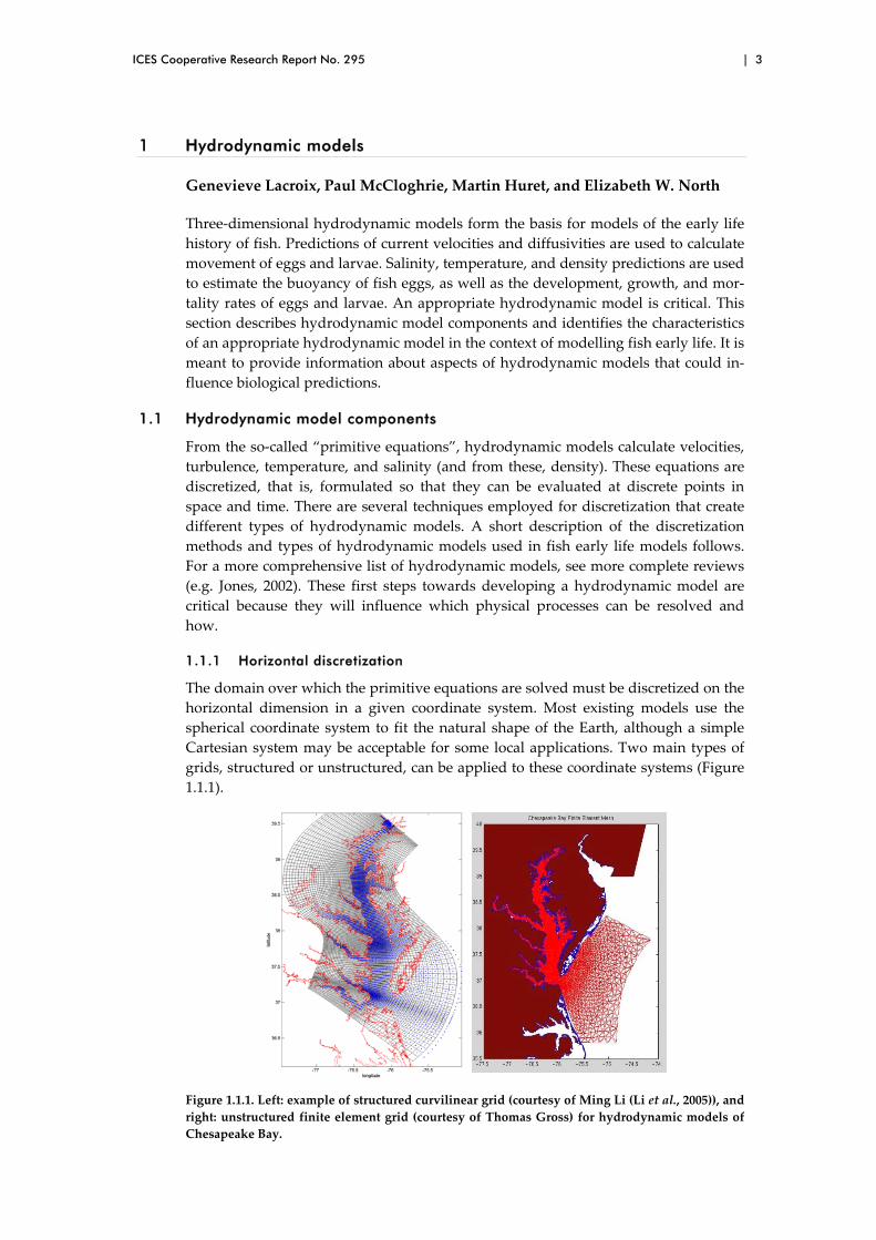
The domain over which the primitive equations are solved must be discretized on the horizontal dimension in a given coordinate system. Most existing models use the spherical coordinate system to fit the natural shape of the Earth, although a simple Cartesian system may be acceptable for some local applications. Two main types of grids, structured or unstructured, can be applied to these coordinate systems (Figure 1.1.1).
Figure 1.1.1. Left: example of structured curvilinear grid (courtesy of Ming Li (Li et al., 2005)), and right: unstructured finite element grid (courtesy of Thomas Gross) for hydrodynamic models of Chesapeake Bay.

4 | Modelling physical–biological interactions during fish early life
A structured grid uses quadrilateral grid cells. In most applications, these grids are approximately rectangular and regular, but possible transformations allow for local refinement in areas of interest (stretched or telescoping grids) and better coastline fitting (curvilinear grid; see Figure 1.1.1, left panel). With this type of grid, equations are solved with the simple and relatively fast finite‐difference method of discretiza‐tion (e.g. Blumberg and Mellor, 1987; Song and Haidvogel, 1994).
The most commonly used structured grids can be subdivided into a number of types (Arakawa, 1966), according to where in each cell the state variables are defined. The most common types are Arakawa‐B and Arakawa‐C grids, and it is important to know which grid type is being used to ensure that the correct interpolation locations are chosen when interpolating from the hydrodynamic output to the locations given by the early life‐history model. An example of an Arakawa‐C grid is given in Figure 1.1.2.
v – horizontal velocity
w – vertical velocity
v – horizontal velocity
w – vertical velocity
density, salinity, temperature
u – horizontal velocity
density, salinity, temperature
u – horizontal velocity
Plan View
Dep
thD
epth
Figure 1.1.2. Schematic of Arakawa‐C grid. Left: plan view, and right, depth view. Locations where water properties are estimated are indicated by coloured symbols. Dashed lines suggest perspective.
The unstructured grid type usually adopts triangular elements (Figure 1.1.1, right panel) and consequently requires other discretization methods to solve the equations, such as the element (variational approach, e.g. Lynch et al., 1996) and finite‐volume (integration approach, e.g. Chen et al., 2006) methods. The flexibility of the unstruc‐tured grids helps resolve complex coastline and bathymetry, and associated proc‐esses, without dramatically increasing the computing time. The formulation of the finite‐volume method ensures mass conservation, as may be the case for finite differ‐ences. Note that the finite‐volume method is not restricted to the unstructured type of grid.
For all types of grids, nesting can be used to work with two different fixed resolu‐tions, allowing refinement in the area of interest. The connection between the two grids is either “one‐way”, where the inner model uses information from the outer model for boundary conditions, or “two‐way”, where both models are dynamically linked.
1.1.2 Vertical discretization
In areas where the water column is consistently vertically well mixed, it may be ad‐visable to use a two‐dimensional model grid (no vertical dimension). However, for most early life‐history models, vertical heterogeneity is important, and three‐dimensional models are required.

ICES Cooperative Research Report No. 295 | 5
There are also three common vertical grid set‐ups. The first is the z‐levels system, where each level represents a fixed depth. The second is the terrain‐following coordi‐nate system (or sigma‐levels), which is also common in coastal applications. Here, each level is a fraction of the total local water‐column depth, allowing for an im‐proved representation of the bottom topography and time‐evolving free surface. The third approach is to use isopycnal coordinates, where each level lies along a density surface, the preferential location of diffusion. This system is generally used for oce‐anic models.
Some vertical coordinate systems employ a hybrid of these methods, one of the goals of which is to avoid the generation of spurious circulation over steep bottom topog‐raphy, which may be encountered when using sigma‐coordinates. Double sigma‐coordinates, where a fixed horizontal layer is specified with a set of sigma‐coordinates above and below, will keep a sufficient refinement of sigma‐layers at the surface when the domain covers both shallow and deep bathymetry. For the same purpose, s‐coordinates, or generalized sigma‐coordinates, use a function of the loca‐tion (and hence bathymetry) to define the sigma‐levels.
1.1.3 Time evolution
Hydrodynamic models predict their state at the next time‐step from their current and prior states. The length of the time‐step is restricted by the size of the grid cells and the speed of propagation of disturbances. This is known as the Courant – Friedrichs –Lewy (CFL) condition. In essence, the time‐step used must be short enough to pre‐vent a disturbance propagating across more than one grid cell in a time‐step. Short time‐steps are required at high spatial resolutions, which can lead to prohibitive computational costs. In order to alleviate this, some models use a technique called “mode splitting”, where the fast (but computationally cheap) barotropic processes (such as the propagation of the tide) are calculated on a short time‐step, whereas the slow baroclinic processes (computationally expensive because they must be calcu‐lated separately for each vertical level) are calculated on a longer time‐step. The baro‐clinic (or internal) time‐step can be as much as 40 times longer than the barotropic (or external) time‐step.
1.1.4 Using hydrodynamic output for particle tracking
Particle‐tracking models use the output of a hydrodynamic model to provide velocity fields. The gridded velocities are interpolated to the position of each particle, and the particles are moved to new locations based on the interpolated velocity and the time‐step of the particle‐tracking model. Particle‐tracking models can be run either online or offline. Running online means that the particle‐tracking calculations are made within the hydrodynamic model program; velocities are calculated, the particles are transported, and then, at the next time‐step, velocities are calculated, particles are transported, and so on. Running offline means that the hydrodynamic model is run once and the velocity fields for the period required are saved. The particle‐tracking model then reads the velocity fields, interpolates, and steps forward in time, then reads the next set of fields. Running online allows the particle‐tracking model to use the velocity fields at the high native resolution (in both space and time) of the hydro‐dynamic model, but it means that each new particle‐tracking experiment requires the hydrodynamic model to be rerun, which can be computationally prohibitive. Al‐though running offline allows output from one hydrodynamic simulation to be used for multiple particle‐tracking simulations, the saved velocity fields will usually be a
6 | Modelling physical–biological interactions during fish early life
lower resolution than the native hydrodynamic model output as a consequence of storage space and read – write speed constraints.
When interpolating gridded velocities to the particle locations, it is important to ac‐count for any horizontal offsets caused by the hydrodynamic grid type. The offsets are usually different for horizontal velocities (u, v), vertical velocities (w), and any scalar properties, such as temperature. This is equally true when interpolating in the vertical.
1.2 Characteristics of an appropriate hydrodynamic model
When assessing whether a hydrodynamic model is appropriate to particle tracking and early life‐history modelling, there are a number of points to consider. Physical processes act on the transport/retention of larvae during their pelagic phase (e.g. wind‐driven circulation, tides, freshwater buoyancy, fronts), on their settlement (e.g. bottom stress), and on conditions affecting larvae survival (e.g. temperature, light). Ensuring that the model (i) covers the domain of interest and (ii) simulates all the key physical processes for both circulation and larval fish (e.g. temperature) is of primary importance. Physical processes with temporal scales close to the time‐scales of fish larvae (e.g. larval stage duration) should be considered. The choice of physical proc‐esses that are to be explicitly resolved should be made by considering the spawning frequency and the larval stage duration, and by taking into account possible links with larval behaviour (e.g. vertical and horizontal migration, feeding processes).
The following list includes some of the physical processes that can affect fish larvae during their pelagic phase and some possible links with larval behaviour. This list, far from being exhaustive, is given to help the modeller choose which physical proc‐esses to consider in the context of the spatio‐temporal scales of the region of interest and the purpose of the study.
• Ocean currents. General circulation, coastal currents, meanders, jets, ed‐dies, shelf‐edge fronts. The main variability is “marine weather” (depres‐sion regimes, storms).
• Tides. Tidal currents (can be important in shallow waters and reefs, de‐pending on the topography), residual circulation, tidal fronts, vertical gra‐dients of horizontal currents. The main variability is (semi‐)diurnal, lunar cycle (spring/neap tides), seasonal cycle (equinoxes, solstices). Possible re‐lationships with “larval behaviour” (synchronization of vertical migration of larvae with ebb – flood tidal cycle), spawning timing (synchronization with spring – neap tidal cycle), and spawning location (spawning depth).
• Freshwater input. Presence of hydrological fronts in the proximity of river mouths, freshwater buoyancy circulation, water stratification density (may act as a barrier to vertical movements), periodic low‐salinity water intru‐sions (may affect depth of larvae). The main variability is (semi‐)diurnal (link with tides), seasonal, and interannual. Relationship with spawning timing (synchronization with high/low river discharges).
• Wind. Wind‐driven circulation, internal waves, Langmuir cells, upwel‐lings/downwellings (and associated fronts and convergences). The main variability is “marine weatherʺ (duration, depression regimes, storms), seasonal (monsoons), and interannual.
• Fronts. Fronts (whatever their origin) can act as a barrier that limits larval transport, but they are also the seat of circulations leading to conver‐
ICES Cooperative Research Report No. 295 | 7
gence/divergence zones. Instabilities (e.g. eddies) can transport “isolated” water masses over long distances.
The size of the model domain and the grid size must be chosen in accordance with the physical processes to be included, the purpose of the study, and the biology of the fish. Processes smaller than the grid size must be parameterized (see Section 1.2.4 Small‐scale physics), and processes acting at scales larger than the model domain should be considered by appropriate boundary conditions (e.g. harmonic tides) or by nesting. The limits of the domain should be chosen sufficiently far from the spawning location(s) and the assumed settlement region(s) to avoid problems related to bound‐ary effects (loss of particles, uncertainties of boundary reflection scheme). For some particular studies, it may be necessary to consider a refined grid (e.g. shallow coastal waters, local retention, heterogeneity of sediment, needs of a fine vertical resolution). Sensitivity studies are recommended to determine the optimal grid resolution (verti‐cal and horizontal). If a refined grid is needed, and if the model domain must encom‐pass a whole region, it is appropriate to consider model nesting.
1.2.1 Boundaries and initial conditions
Close to their open (wet) boundaries, the predictions from hydrodynamic models are strongly influenced by the conditions imposed on the model at the boundaries. For example, baroclinic velocities depend on the density structure of the water, that is, both temperature and salinity. Surface temperatures will usually decrease close to dynamic equilibrium within days as a result of rapid heat exchange with the atmos‐phere, whereas bottom temperatures in stratified water may take much longer. Salini‐ties in non‐coastal areas can remain dominated by boundary effects throughout the model domain. Fortunately, when considering large areas, salinity gradients can of‐ten be accurately reproduced, although the absolute values may be incorrect. Baro‐tropic velocities, driven by tidal boundary conditions, usually propagate through the entire model domain.
When choosing the extent of the model domain, it is important to exceed the area of interest for the tracking model because of the influence of boundary conditions on the model predictions. Boundary condition data are usually given at lower resolution and may be derived from a climatology rather than for the specific dates being simu‐lated. These boundary values then propagate their influence into the model domain for a distance that is a factor of the local flow rates and the rate at which the values are modified to fit with the internal dynamics. The key to accurate representation is, therefore, using high‐quality data on the boundaries and undertaking a careful vali‐dation process.
The same considerations need to be applied to the initial conditions for the hydrody‐namic model. The period during which initialization effects are significant is a factor of the rate of change of the variables. To avoid initialization effects, a hydrodynamic model is usually “spun up” for a period of time before the outputs are used. For baro‐tropic velocities, this may only require a couple of weeks; however, for baroclinic ve‐locities, it will usually take months. Because of the slow rate of adjustment of temperature and salinity in stratified bottom waters and seasonally stratified areas, hydrodynamic models are usually spun up during winter.
1.2.2 Resolution
The choice of model resolution is usually strongly influenced by the available com‐puter resources. Higher horizontal resolution allows models to resolve more of the

8 | Modelling physical–biological interactions during fish early life
physical processes. However, a doubling of horizontal resolution implies an eightfold increase in computational expense. (The factor of eight comes from a doubling in the x, y, and time dimensions. The requirement for shorter time‐steps at higher resolution comes from the CFL condition). When an improvement in the resolution is not neces‐sary over the whole domain, curvilinear and unstructured grids allow the resolution to be location‐dependent (which does not remove the constraint on the time‐step, but does reduce the number of cells over which the calculations are made).
The ability to resolve the mesoscale is a significant improvement gained from higher resolution. The size of mesoscale features (eddies, etc.) is determined by the local Rossby radius (L), which can be calculated from
L=√gH/f,
where H is the water depth, f is the Coriolis parameter, i.e. 2 × 7.29 × 10 −5 × sin (lati‐tude), and g is the reduced gravity at the pycnocline. A typical shelf‐sea mesoscale eddy at 55° N will have a diameter of roughly 20 km. To resolve this eddy, a hydro‐dynamic model will need to have six to ten grid points across the eddy and therefore a resolution of at least 3 km.
1.2.3 Model validation
Only thoroughly validated hydrodynamic models, including all key physical proc‐esses, should be used for particle‐tracking studies. The modeller should at least verify that current velocity (horizontal and vertical) and/or trajectory paths are correctly simulated. After that, depending on the situation or the purpose of the study, particu‐lar attention should be paid to the accuracy of additional parameters, such as salinity (regions of freshwater influence), light attenuation (predator‐avoidance behaviour), temperature (if temperature‐dependent processes are considered), and bottom stress (settlement). Model error quantification techniques include cost functions (Delhez et al., 2004; Radach and Moll, 2006), root‐mean‐square error of modelled vs. observed values, model skill scores (Warner et al., 2005), and Taylor diagrams (Taylor, 2001).
Sensitivity studies (combined with validation) should allow the modeller to deter‐mine the degree of importance of the physical processes and help when choosing the key processes to include, according to the purpose of the study and the larval behav‐iour considered (e.g. Hill, 1994; Lefebvre et al., 2003; Ellien et al., 2004; Sentchev and Korotenko, 2004).
1.2.4 Small-scale physics
In hydrodynamic modelling, processes that occur at scales too small for the model resolution to simulate accurately are parameterized to allow for their diffusive effect on the large‐scale structure. (Note that models require a resolution in excess of five times the scale of a feature in order to be able to resolve the feature.) The parameter used is known as the “eddy diffusivity” and accounts for unresolved advective proc‐esses, such as frontal instabilities, steering by unresolved topographic features, and sea breezes. Omission of physical processes generally requires an increase in the specified eddy diffusivity. This parameter also depends largely on the method used to solve the advection equations. Low‐order methods are inherently more diffusive than higher order approximations. In many cases, this numerical diffusion is enough to account for small‐scale processes; however, additional diffusion is often added to improve model stability.

ICES Cooperative Research Report No. 295 | 9
2 Particle tracking
David Brickman, Bjørn Ådlandsvik, Uffe H. Thygesen, Carolina Parada, Kenneth Rose, Albert J. Hermann, and Karen Edwards
Particle‐tracking models form the backbone of three‐dimensional models of fish early life. These models use predictions of current velocities and diffusivities from hydro‐dynamic models to calculate the movement of individual particles in space and time. The goal of this section is to provide a set of recommendations for particle tracking in estuary and ocean modelling. Because the motivation comes principally from its ap‐plication to biophysical modelling, the case of biologically active particles is specifi‐cally considered. The first part of this section presents, in a concise form, the essential aspects of best practices for particle tracking. Extra material is contained in Annexes 1 − 5. The second part presents a number of cases designed to test the performance of a particle‐tracking routine.
2.1 Best practices for particle tracking
What makes particle tracking in an oceanographic (biophysical modelling) context different from tracking in an atmospheric context? The simple answer is that, histori‐cally, development of particle‐tracking theory and techniques in the atmosphere was concerned principally with the atmospheric boundary layer, with an emphasis on correctly describing the statistics of dispersion for time‐scales shorter than the La‐grangian time‐scale (TL), the time‐scale at which velocity fluctuations are correlated. Generally, the computations were done for short periods (minutes to hours) and in one or two dimensions (for which analytic models exist; see Wilson et al., 1981; Legg and Raupach, 1982; Thomson, 1987). These Lagrangian stochastic models (LSMs), or “random flight models”, are mathematically complicated, but are valid at all time scales (except below the Kolmogorov microscale, where viscosity becomes relevant; Thomson, 1987; Rodean, 1996). In addition, a critical problem of buoyant particles, “the trajectory crossing problem”, has only approximate solutions for LSMs (Sawford and Guest, 1991; Olia, 2002).
For biophysical modelling in the aquatic realm, we tend to be interested in time‐scales longer than TL and in three‐dimensional drift for periods as long as several months. Another crucial difference is that many biophysical particles (representing planktonic larvae) have directed swimming motions that must be incorporated into the particle‐tracking algorithm. This necessitates the use of random displacement models (RDMs, also known as random walk models). These models are valid for time‐scales >> TL (TL vertical = 3 – 10 min; TL horizontal = 1 – 8 d (near surface; greater at depth)). That the time‐scales of interest in the ocean are not always >> TL (especially on the horizontal plane) means that the use of RDMs in oceanographic particle track‐ing can be considered a “best‐we‐can‐do” approach.
2.1.1 Choice of model
For the reasons outlined above, an RDM is recommended for oceanographic applica‐tion. If we assume that the turbulence at each point is isotropic in the horizontal (i.e. its local statistics are invariant to rotations around a vertical axis), then turbulence is characterized by the horizontal diffusivity K11 = K22 and the vertical diffusivity K33. The three‐dimensional RDM then becomes (Rodean, 1996):
10 | Modelling physical–biological interactions during fish early life
iiii
iiii QdttxKdt
xtxK
txUdx 2/1)),(2(),(
),( +⎥⎦
⎤⎢⎣
⎡∂
∂+= ,
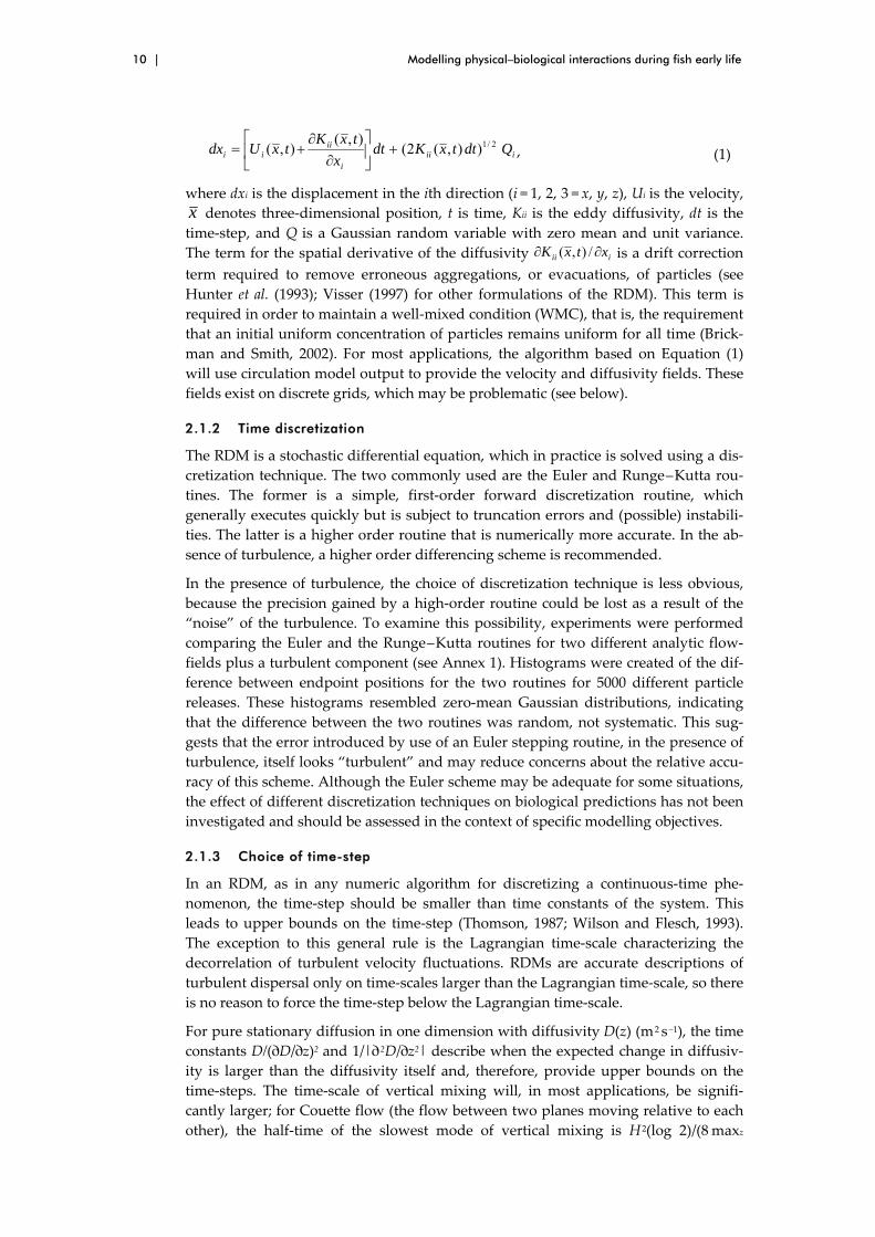
(1)
where dxi is the displacement in the ith direction (i = 1, 2, 3 = x, y, z), Ui is the velocity, x denotes three‐dimensional position, t is time, Kii is the eddy diffusivity, dt is the time‐step, and Q is a Gaussian random variable with zero mean and unit variance. The term for the spatial derivative of the diffusivity iii xtxK ∂∂ /),( is a drift correction term required to remove erroneous aggregations, or evacuations, of particles (see Hunter et al. (1993); Visser (1997) for other formulations of the RDM). This term is required in order to maintain a well‐mixed condition (WMC), that is, the requirement that an initial uniform concentration of particles remains uniform for all time (Brick‐man and Smith, 2002). For most applications, the algorithm based on Equation (1) will use circulation model output to provide the velocity and diffusivity fields. These fields exist on discrete grids, which may be problematic (see below).
2.1.2 Time discretization
The RDM is a stochastic differential equation, which in practice is solved using a dis‐cretization technique. The two commonly used are the Euler and Runge – Kutta rou‐tines. The former is a simple, first‐order forward discretization routine, which generally executes quickly but is subject to truncation errors and (possible) instabili‐ties. The latter is a higher order routine that is numerically more accurate. In the ab‐sence of turbulence, a higher order differencing scheme is recommended.
In the presence of turbulence, the choice of discretization technique is less obvious, because the precision gained by a high‐order routine could be lost as a result of the “noise” of the turbulence. To examine this possibility, experiments were performed comparing the Euler and the Runge – Kutta routines for two different analytic flow‐fields plus a turbulent component (see Annex 1). Histograms were created of the dif‐ference between endpoint positions for the two routines for 5000 different particle releases. These histograms resembled zero‐mean Gaussian distributions, indicating that the difference between the two routines was random, not systematic. This sug‐gests that the error introduced by use of an Euler stepping routine, in the presence of turbulence, itself looks “turbulent” and may reduce concerns about the relative accu‐racy of this scheme. Although the Euler scheme may be adequate for some situations, the effect of different discretization techniques on biological predictions has not been investigated and should be assessed in the context of specific modelling objectives.
2.1.3 Choice of time-step
In an RDM, as in any numeric algorithm for discretizing a continuous‐time phe‐nomenon, the time‐step should be smaller than time constants of the system. This leads to upper bounds on the time‐step (Thomson, 1987; Wilson and Flesch, 1993). The exception to this general rule is the Lagrangian time‐scale characterizing the decorrelation of turbulent velocity fluctuations. RDMs are accurate descriptions of turbulent dispersal only on time‐scales larger than the Lagrangian time‐scale, so there is no reason to force the time‐step below the Lagrangian time‐scale.
For pure stationary diffusion in one dimension with diffusivity D(z) (m 2 s −1), the time constants D/(∂D/∂z)2 and 1/|∂ 2D/∂z2| describe when the expected change in diffusiv‐ity is larger than the diffusivity itself and, therefore, provide upper bounds on the time‐steps. The time‐scale of vertical mixing will, in most applications, be signifi‐cantly larger; for Couette flow (the flow between two planes moving relative to each other), the half‐time of the slowest mode of vertical mixing is H 2(log 2)/(8 maxz
ICES Cooperative Research Report No. 295 | 11
(D(z))), where H is the water depth. This time‐scale can be used as a rough measure of vertical mixing in other flows as well, or more accurate time‐scales can be obtained analytically or numerically for the specific flow.
Additional time‐scales may characterize horizontal motion or other (e.g. biophysical) processes. The chosen time‐step must ensure that all processes are accurately re‐solved. For an example of the effects of different choices of time‐step see Annex 2.
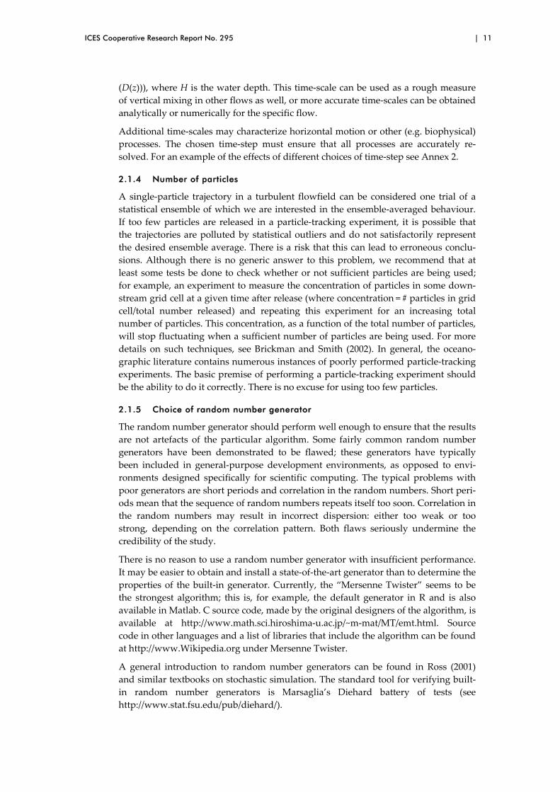
2.1.4 Number of particles
A single‐particle trajectory in a turbulent flowfield can be considered one trial of a statistical ensemble of which we are interested in the ensemble‐averaged behaviour. If too few particles are released in a particle‐tracking experiment, it is possible that the trajectories are polluted by statistical outliers and do not satisfactorily represent the desired ensemble average. There is a risk that this can lead to erroneous conclu‐sions. Although there is no generic answer to this problem, we recommend that at least some tests be done to check whether or not sufficient particles are being used; for example, an experiment to measure the concentration of particles in some down‐stream grid cell at a given time after release (where concentration = # particles in grid cell/total number released) and repeating this experiment for an increasing total number of particles. This concentration, as a function of the total number of particles, will stop fluctuating when a sufficient number of particles are being used. For more details on such techniques, see Brickman and Smith (2002). In general, the oceano‐graphic literature contains numerous instances of poorly performed particle‐tracking experiments. The basic premise of performing a particle‐tracking experiment should be the ability to do it correctly. There is no excuse for using too few particles.
2.1.5 Choice of random number generator
The random number generator should perform well enough to ensure that the results are not artefacts of the particular algorithm. Some fairly common random number generators have been demonstrated to be flawed; these generators have typically been included in general‐purpose development environments, as opposed to envi‐ronments designed specifically for scientific computing. The typical problems with poor generators are short periods and correlation in the random numbers. Short peri‐ods mean that the sequence of random numbers repeats itself too soon. Correlation in the random numbers may result in incorrect dispersion: either too weak or too strong, depending on the correlation pattern. Both flaws seriously undermine the credibility of the study.
There is no reason to use a random number generator with insufficient performance. It may be easier to obtain and install a state‐of‐the‐art generator than to determine the properties of the built‐in generator. Currently, the “Mersenne Twister” seems to be the strongest algorithm; this is, for example, the default generator in R and is also available in Matlab. C source code, made by the original designers of the algorithm, is available at http://www.math.sci.hiroshima‐u.ac.jp/~m‐mat/MT/emt.html. Source code in other languages and a list of libraries that include the algorithm can be found at http://www.Wikipedia.org under Mersenne Twister.
A general introduction to random number generators can be found in Ross (2001) and similar textbooks on stochastic simulation. The standard tool for verifying built‐in random number generators is Marsaglia’s Diehard battery of tests (see http://www.stat.fsu.edu/pub/diehard/).
12 | Modelling physical–biological interactions during fish early life
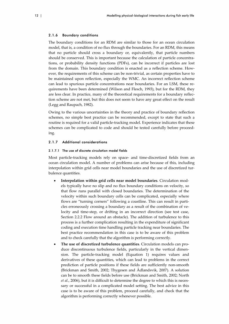
2.1.6 Boundary conditions
The boundary conditions for an RDM are similar to those for an ocean circulation model, that is, a condition of no flux through the boundaries. For an RDM, this means that no particle should cross a boundary or, equivalently, that particle numbers should be conserved. This is important because the calculation of particle concentra‐tions, or probability density functions (PDFs), can be incorrect if particles are lost from the domain. This boundary condition is enacted as a reflection scheme. How‐ever, the requirements of this scheme can be non‐trivial, as certain properties have to be maintained upon reflection, especially the WMC. An incorrect reflection scheme can lead to spurious particle concentrations near boundaries. For an LSM, these re‐quirements have been determined (Wilson and Flesch, 1993), but for the RDM, they are less clear. In practice, many of the theoretical requirements for a boundary reflec‐tion scheme are not met, but this does not seem to have any great effect on the result (Legg and Raupach, 1982).
Owing to the various uncertainties in the theory and practice of boundary reflection schemes, no simple best practice can be recommended, except to state that such a routine is required for a valid particle‐tracking model. Experience indicates that these schemes can be complicated to code and should be tested carefully before proceed‐ing.
2.1.7 Additional considerations
2.1.7.1 The use of discrete circulation model fields
Most particle‐tracking models rely on space‐ and time‐discretized fields from an ocean circulation model. A number of problems can arise because of this, including interpolation within grid cells near model boundaries and the use of discretized tur‐bulence quantities.
• Interpolation within grid cells near model boundaries. Circulation mod‐els typically have no slip and no flux boundary conditions on velocity, so that flow runs parallel with closed boundaries. The determination of the velocity within such boundary cells can be complicated, especially where flows are “turning corners” following a coastline. This can result in parti‐cles erroneously crossing a boundary as a result of the combination of ve‐locity and time‐step, or drifting in an incorrect direction (see test case, Section 2.2.2 Flow around an obstacle). The addition of turbulence to this process is a further complication resulting in the expenditure of significant coding and execution time handling particle tracking near boundaries. The best practice recommendation in this case is to be aware of this problem and to check carefully that the algorithm is performing correctly.
• The use of discretized turbulence quantities. Circulation models can pro‐duce discontinuous turbulence fields, particularly in the vertical dimen‐sion. The particle‐tracking model (Equation 1) requires values and derivatives of these quantities, which can lead to problems in the correct prediction of particle positions if these fields are sufficiently non‐smooth (Brickman and Smith, 2002; Thygesen and Ådlandsvik, 2007). A solution can be to smooth these fields before use (Brickman and Smith, 2002; North et al., 2006), but it is difficult to determine the degree to which this is neces‐sary or successful in a complicated model setting. The best advice in this case is to be aware of this problem, proceed carefully, and check that the algorithm is performing correctly whenever possible.

ICES Cooperative Research Report No. 295 | 13
2.1.7.2 Backwards particle tracking
In problems of egg/larval drift, we often have an estimate of the distribution of eggs or larvae, provided by survey data, but incomplete knowledge of the release area of the propagules. In other words, we often have more data at the endpoint than at the starting point. One benefit of the particle‐tracking technique is the ability to reverse time and perform backward particle tracking in order to find the most likely origin for observed propagules. For example, we consider the case of truly planktonic parti‐cles in a flowfield u that is divergence‐free and does not cross boundaries. In this case, it is reasonable to use the simple one‐dimensional, time‐reversed, Euler scheme:
QdtxKdtxKdtxuxx ttttdtt )(2)()( +∇+−=− , (2)
where Q has the same meaning as in Equation (1). Starting from the final position and time (xf, tf) when the simulation reaches the starting time t0, the density of larvae at any position x0 will be proportional to the likelihood function of the initial condition x0, viewed as an unknown parameter. (For more details on this example, see Thyge‐sen, in prep.). Other papers on biophysical backward particle tracking include Batchelder (2006) and Christensen et al. (2007). A paper to be recommended from the atmospheric literature is Flesch et al. (1995).
2.1.7.3 Coupling particle tracking with continuous fields from NPZ models
There are several issues to consider when coupling particle‐tracking models to the continuous fields generated by nutrient‐phytoplankton‐zooplankton (NPZ) models. The continuous fields are the spatially explicit, physics‐related outputs (e.g. velocities used for advection‐diffusion movement of the particles) and biologically related out‐puts (e.g. zooplankton densities as prey for the particles) generated by the NPZ model. Some of these issues relate to the quality of these continuous fields, whereas other issues relate to the mechanics of how the particles are coupled to the fields.
The first issue is the quality of the outputted fields from the NPZ, including the over‐all stability of the NPZ model, the realism of the NPZ‐related parameter values, the formulation of the predation‐closure terms used to impose mortality on the zoo‐plankton, and the information on model performance provided by data assimilation and validation efforts (see Annex 3).
The second issue also influences the quality of the fields and involves the way in which the NPZ submodel is coupled to the physics model. Issues such as whether the NPZ is run online or offline with the physics, and the compatibility of the spatial and temporal resolutions between the NPZ and physics models, affect the realism and quality of the outputted NPZ fields (see Annex 4).
The third issue relates to how the particles are coupled to the NPZ fields (see Annex 5), for example, whether or not a sufficient number of particles (e.g. larval fish) are followed in order to properly represent their interactions with prey patchiness, the fact that one‐way coupling prevents trophic feedback from the particles to their prey and from prey exhibiting avoidance behaviours or other responses, and the degree to which movement of particles (e.g. larval fish) is purely physics‐driven or involves active behaviour (e.g. vertical migration, swimming). Addressing the patchiness, tro‐phic feedback, and prey‐response issues requires the NPZ and particle‐tracking mod‐els to be solved simultaneously using a large number of particles. How to meld advective and behaviour modes of movement remains an open question. Both the active behaviour of the particles and the reactions of the prey can change the trajecto‐ries of the particles (individuals in the model) and the predicted densities of the prey.

14 | Modelling physical–biological interactions during fish early life
2.2 Test cases
In this section, we present a number of test cases designed to test the performance of a particle‐tracking routine and illustrate problems that can arise when interpolating near boundaries.
2.2.1 Vertical distribution of buoyant particles
2.2.1.1 Purpose
The purpose is to test how well the particle‐tracking code handles buoyant particles, especially in relationship to the surface and bottom boundary conditions.
2.2.1.2 Background
The need to handle non‐neutral particles arises in many applications, including phytoplankton, sediments, or, in this test case, fish eggs. The stationary case was treated by Sundby (1983). The general problem is easily handled in the Eulerian (con‐centration‐based) setting. A Matlab toolbox was developed by Ådlandsvik (2000). This point of view has been adopted for the sampling of anchovy and sardine eggs using the Continuous Underwater Fish Egg Sampler (CUFES; Boyra et al., 2003). For particle tracking, the binned random walk part of this test case was given by Thyge‐sen and Ådlandsvik (2007).
2.2.1.3 Analytical solution
This test case considers a one‐dimensional water column with non‐neutral particles with a buoyant velocity w and eddy diffusivity K. The vertical coordinate z points upwards, with z = 0 at bottom and z = H at the surface. The concentration φ of parti‐cles is governed by the Eulerian conservation law,
⎟⎠⎞
⎜⎝⎛
∂∂
∂∂
=∂∂
+∂∂
zK
zw
ztφφφ )(
. (3)
The boundary conditions are zero flux through the surface:
Hzz
Kw ,0, =∂∂
=φφ .
(4)
The solution evolves towards a stationary solution where the flux is zero in the whole water column. With constant coefficients, this ordinary differential equation gives a truncated exponential distribution. With m = w/K and a vertical integrated concentra‐tion Φ, this can be written
mzmH e
em
1−Φ=φ .
(5)
This has mean height above bottom
1
1−
+−= mHeH
mHμ
, (6)
and variance
2
2
222
)1(222 μσ −
−−−−
= mH
mH
emmHHme
. (7)
Further details are given in Sundby (1983) and Ådlandsvik (2000).

ICES Cooperative Research Report No. 295 | 15
2.2.1.4 Specification
The specific values used for this test case are given in Table 2.2.1. These values give a stationary mean depth (from surface) of 9.25 m and a standard deviation of 8.34 m. The particles are released 12.5 m above bottom, and the simulation time is 48 h.
Table 2.2.1. Variable settings for the buoyant test case.
VARIABLE VALUE UNIT
H 40 m w 0.001 m s−1 K 0.01 m s−2
2.2.1.5 Continuous random walk model
The continuous random walk model (i.e. RDM) for this problem with constant coeffi‐cients is implemented in a Euler – Forward fashion by,
QtKtwZZ nn Δ+Δ+=+ 21 , (8)
where Z is displacement and Q is a random variable with zero mean and unit vari‐ance. The boundary conditions are more difficult; the usual reflective boundary scheme at the surface,
11 2 ++ −← nn ZHZ 1, if Zn+1 >H, (9)
corresponds to
0=
∂∂
zφ ,
(10)
which differs from the correct boundary condition in Equation (4). In fact, the ana‐lytical stationary solution has the maximum of the derivative at the surface.
The number of particles in this test case is 40 000. Two different time‐steps, 5 and 30 min, are considered, and a Gaussian distribution is used for the random walk. The 5 min case has also been run with a uniform (top‐hat) distribution for the random component. The reflective boundary condition is applied. For the plot, the particles have been counted in 1 m bins.
The result demonstrates that the RDM solutions are good (Figure 2.2.1) except when they are close to the surface, where they underestimate the concentration. The height of the boundary zone depends on when the particle movement is influenced by the boundary, that is, the length scales w∆t and √2K∆t. In this case, the shape of the ran‐dom walk distribution influences the result, where the Gaussian shape is superior to the top‐hat. This is probably caused by the top‐hat distribution giving higher prob‐abilities further from the mean, making the random walk “feel” the boundary at longer distance.
2.2.1.6 Binned random walk
The binned random walk does not have boundary problems because it is constructed by finite volume methods for the advection‐diffusion equation (see Thygesen and Ådlandsvik, 2007). The water column was discretized into eight uneven bins, with

16 | Modelling physical–biological interactions during fish early life
depths of 10, 5, 5, 5, 5, 5, 3, and 2 m, counted from the bottom. The time‐step used was 5 min, and both the first‐order upstream and a second‐order scheme were con‐sidered. The results are given in Figure 2.2.2. This figure also shows the analytical solution, averaged into the same bins. The upstream solution shows too much mix‐ing: underestimating the concentration near the surface and overestimating it near the bottom. The second‐order method follows the analytical solution well but over‐shoots near the surface.
Figure 2.2.1. Results for the continuous random walk model.
Figure 2.2.2. Results for the binned random walk model.
2.2.2 Flow around an obstacle
2.2.2.1 Purpose
The purpose is to test how different horizontal advection implementations handle a curved flowfield and a land obstacle.
2.2.2.2 Background
Non‐rotational flow around a cylinder is one of the classical examples considered in almost all hydrodynamics textbooks. Of particular interest is the book by Bennett (2006), which takes a Lagrangian point of view.
2.2.2.3 Analytical considerations
The example is considered in a coastal oceanographic setting; the cylinder becomes a circular island. As the example is symmetric, only the upper half is considered. That

ICES Cooperative Research Report No. 295 | 17
is, we consider a straight coast at y = 0 with ocean in the upper half plane (y > 0) and with a half‐circular peninsula with centre (x0, 0) and radius R.
The steady non‐rotational flow is given by a stream function
yu
yxxyRu
0220
20
)(−
+−=ψ ,
(11)
where u0 is the along‐coast velocity far from the obstacle. The stream function is nor‐malized so that the land boundary is given by the contour ψ = 0. The flow follows the streamlines, that is, isolines of ψ with higher values to the right, more precisely
222
0
2202
00 ))(()(
yxxyxxRuu
yu
+−−−
−=∂∂
−=ψ
(12)
and
222
0
020 ))((
)(2yxxyxxRu
xv
+−−
−=∂∂
=ψ
. (13)
According to Bennett (2006), it is unlikely that analytical expressions will be found for the time‐dependent particle movement in this example. Bennet does, however, pro‐vide an analytical description of stream lines. The “exact” solution shown below is obtained by using converged Runge – Kutta with a small time‐step (36 s), using the analytical expression above for the velocities without interpolation. The dashed stream lines are simply obtained by contouring the discretized version of the stream function.
2.2.2.4 Specification
A domain of length L along the coast and width W is considered. The peninsula centre is at x = 0.5 L and the radius R = 0.32 W. The numerical values are specified in Table 2.2.2.
Table 2.2.2. Variable settings for the peninsula test case.
Variable Value Unit
L 100 km W 50 km u0 1 m s−1
The domain is discretized by ∆x = ∆y = 1 km. The grid coordinates are chosen so that grid cell (i, j) has its centre at (x, y) = (i∆x, j∆x) for i = 0, . . . , 99 and j = 0, . . . , 49. The velocities are sampled in an A‐grid, that is, in the grid centres. Denoting the velocity arrays U and V, we have
U(i, j) = u(i∆x, j∆x), V(i, j) = v(i∆x, j∆x), (14)
where u and v are given by the analytical formulas above. The velocities are set to zero at land, that is, where ψ ≤ 0, in particular U (i, 0) = V (i, 0) = 0. The initial particle distribution is 1000 particles on a line perpendicular to the coast:
Xk = 3, Yk = 0.45 + 0.045k for k = 1, . . . ,1000. (15)
The simulation time is 24 h, for which the particles would be transported 86.4 km with the reference velocity u0.

18 | Modelling physical–biological interactions during fish early life
2.2.2.5 Simulations
The first‐order Euler forward and the Runge – Kutta fourth‐order method are consid‐ered. Both methods are used here with bilinear interpolation to interpolate from the grid‐cell centres to the particle positions. The treatment of boundaries is simple, with the zero land velocity interpolated to the particle position and no reflection scheme implemented. This procedure may leave particles on land, but in the absence of tur‐bulence, this was not considered to be important. A time‐step of 1 h was used for both methods. The results from this test are presented in Figure 2.2.3. Far from the peninsula, both methods recapture the exact solution (green, red, and black symbols overlap). Close to the peninsula, the Euler method fails, leaving a trail of particles clearly separated from the peninsula. The Runge – Kutta method performs better, leaving a tiny tail of particles very close to the peninsula that do not overlap those produced by the exact solution.
Figure 2.2.3. Peninsula test case.
The velocities from the formulas above are also defined for ψ > 0, giving a circulation within the “peninsula”. Using these velocities in the interpolation and intermediate Runge – Kutta steps gives a reference solution with ideal land treatment. This land treatment makes the Runge – Kutta indistinguishable from the exact solution and also improves the results from the Euler method. These results are shown in Figure 2.2.4 in which symbols for the Runge–Kutta method overlap those of the exact solution.
Figure 2.2.4. Peninsula test case with circulation within the “peninsula”.

ICES Cooperative Research Report No. 295 | 19
2.2.2.6 Comment
This test was designed to demonstrate the difference between the Euler method and higher order methods, such as Runge – Kutta, and to point out problems associated with interpolation near boundaries. No random walk diffusion has been applied, which could reduce the advantage of higher order methods (see Annex 1). Also, shorter time‐steps improve the performance of both models and may decrease the difference between them.

20 | Modelling physical–biological interactions during fish early life
3 Biological processes
3.1 Initial conditions: spawning locations
Alejandro Gallego and Elizabeth W. North
The starting position of particles in a heterogeneous flowfield fundamentally controls the direction and distance of particle transport. Therefore, the space and time struc‐tures of spawning patterns (where, when, and what magnitude) are the initial condi‐tions for individually based models of fish early life that begin with egg stages. Initial conditions differ in degree of complexity, depending on the objective of the model‐ling effort. For example, interannual differences in the magnitude of egg production are needed for predicting recruitment variability but may not be necessary for under‐standing transport pathways between spawning and settlement areas.
Ideally, fine‐scale information on spatial and temporal patterns in spawning is needed to initialize models (e.g. frequent surveys of egg distribution and abundance throughout a spawning area over multiple years). However, this information is often limited or non‐existent. Therefore, an estimate of initial conditions is needed. In the most basic formulation, randomly distributed particles could be released within the spawning area throughout the duration of the spawning time window. This may provide information about all possible trajectories through space and time, but not the actual trajectories of the simulated populations in each year because spawning times, locations, and magnitudes vary from year to year. For simulating the magni‐tude and timing of spawning events, egg‐production models are often required (see Section 3.1.1 Egg‐production models).
When incorporating initial conditions into models, the following questions should be asked (C. Mullon, pers. comm.): what are the spawning patterns that: (i) emerge from observations, (ii) can be modelled with simple assumptions on individual behaviour, and (iii) could be related to different regimes of population dynamics? Several factors should be considered (C. Mullon, pers. comm.).
• Spatial structure of spawning. Spawning locations/features can affect the population structure in a way that can be modelled. With information on different spawning features, the model can predict the spatial distribution of recruits and allow identification of the ways in which behavioural proc‐esses may be mediated by environmental conditions, parental condition, and gregarious behaviour.
• Time structure of spawning. Spawning features can be related to envi‐ronmental conditions. With observations of spawning events (space, time) and observed concomitant environmental parameters, modelling results can be used to determine if individual spawners use environmental cues to optimize their reproductive success (fitness).
• Evolutionary processes. Spawning behaviour is the result of an evolution‐ary process. With different sets of constraints that affect fitness and taking account of the spawning choices of individuals, predicted spawning pat‐terns can be analysed to understand how evolutionary processes influence opportunism, natal homing, and bet‐hedging strategies.
See Mullon et al. (2002), Grimm and Railsback (2005), and Jørgensen et al. (2008) for additional information.
ICES Cooperative Research Report No. 295 | 21
3.1.1 Egg-production models
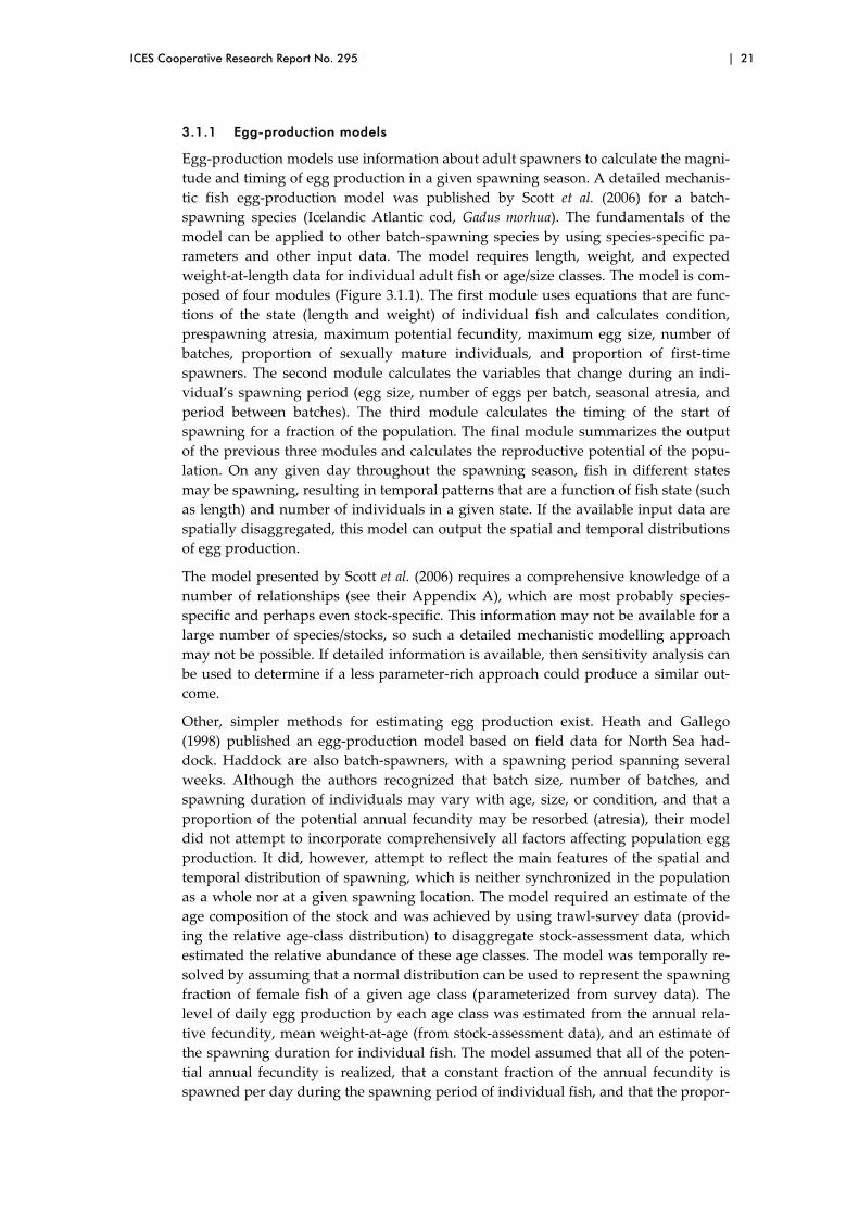
Egg‐production models use information about adult spawners to calculate the magni‐tude and timing of egg production in a given spawning season. A detailed mechanis‐tic fish egg‐production model was published by Scott et al. (2006) for a batch‐spawning species (Icelandic Atlantic cod, Gadus morhua). The fundamentals of the model can be applied to other batch‐spawning species by using species‐specific pa‐rameters and other input data. The model requires length, weight, and expected weight‐at‐length data for individual adult fish or age/size classes. The model is com‐posed of four modules (Figure 3.1.1). The first module uses equations that are func‐tions of the state (length and weight) of individual fish and calculates condition, prespawning atresia, maximum potential fecundity, maximum egg size, number of batches, proportion of sexually mature individuals, and proportion of first‐time spawners. The second module calculates the variables that change during an indi‐vidual’s spawning period (egg size, number of eggs per batch, seasonal atresia, and period between batches). The third module calculates the timing of the start of spawning for a fraction of the population. The final module summarizes the output of the previous three modules and calculates the reproductive potential of the popu‐lation. On any given day throughout the spawning season, fish in different states may be spawning, resulting in temporal patterns that are a function of fish state (such as length) and number of individuals in a given state. If the available input data are spatially disaggregated, this model can output the spatial and temporal distributions of egg production.
The model presented by Scott et al. (2006) requires a comprehensive knowledge of a number of relationships (see their Appendix A), which are most probably species‐specific and perhaps even stock‐specific. This information may not be available for a large number of species/stocks, so such a detailed mechanistic modelling approach may not be possible. If detailed information is available, then sensitivity analysis can be used to determine if a less parameter‐rich approach could produce a similar out‐come.
Other, simpler methods for estimating egg production exist. Heath and Gallego (1998) published an egg‐production model based on field data for North Sea had‐dock. Haddock are also batch‐spawners, with a spawning period spanning several weeks. Although the authors recognized that batch size, number of batches, and spawning duration of individuals may vary with age, size, or condition, and that a proportion of the potential annual fecundity may be resorbed (atresia), their model did not attempt to incorporate comprehensively all factors affecting population egg production. It did, however, attempt to reflect the main features of the spatial and temporal distribution of spawning, which is neither synchronized in the population as a whole nor at a given spawning location. The model required an estimate of the age composition of the stock and was achieved by using trawl‐survey data (provid‐ing the relative age‐class distribution) to disaggregate stock‐assessment data, which estimated the relative abundance of these age classes. The model was temporally re‐solved by assuming that a normal distribution can be used to represent the spawning fraction of female fish of a given age class (parameterized from survey data). The level of daily egg production by each age class was estimated from the annual rela‐tive fecundity, mean weight‐at‐age (from stock‐assessment data), and an estimate of the spawning duration for individual fish. The model assumed that all of the poten‐tial annual fecundity is realized, that a constant fraction of the annual fecundity is spawned per day during the spawning period of individual fish, and that the propor‐

22 | Modelling physical–biological interactions during fish early life
tion of spawning females of a given age class in the population can be described by a normal distribution centred on the date of peak spawning.
In cases where the information (data, parameters, and functional relationships) re‐quired for the modelling approaches described above is not available, information about the peak and variability of spawning at a given location may be sufficient to give approximate daily egg production. For example, a normal distribution with the mean equal to the peak spawning date could be used, along with a spawning season that would correspond to two standard deviations, as long as there is an estimate of total spawning (directly from stock assessment or from estimates of spawning‐stock biomass and a weight – fecundity relationship).
Some of the modelling approaches (e.g. those described above) may result in distri‐butions of spawning with unrealistically long “tails”, which would imply that some spawning takes place well outside the observed spawning season. A practical solu‐tion is to establish a cut‐off threshold (e.g. based on field observations), outside of which egg production is considered negligible and ignored. For accuracy, the egg production that would have taken place at the tails should be redistributed within the accepted distribution of spawning.
In the absence of sufficient data/information to model egg production or the distribu‐tion of spawning, it may be possible to use data on the observed distribution of larvae to identify the timing and location of spawning. Of course, this approach is only valid if the sampling covers the full geographical domain occupied by the larvae of the species of interest, and if estimates of the age and mortality of the eggs and larvae are available. Knowledge of the duration of the egg stage is necessary to identify the spawning location of pelagic eggs. Information on the mortality level experienced by the eggs and larvae is needed if quantitative estimates of spawning are required. Unless we are dealing with very young larvae of demersal‐spawning species (or with a very short egg‐stage duration), where we may choose to disregard transport from the spawning grounds, we need to account for transport processes from spawning to sampling. To do so, the biophysical model can be run backwards (see Section 2.1.7 Additional considerations; Batchelder, 2006; Christensen et al., 2007), or a forward‐running model may be used, covering at least all possible spawning sites over at least the full duration of spawning.
When using an egg‐production model to provide initial conditions for a particle‐tracking model, the spatial and temporal resolution of the hydrodynamic and parti‐cle‐tracking models should be kept in mind. Egg‐production models often provide continuous predictions (e.g. a continuous function in time), although data used to force the model are of coarse resolution (e.g. length – weight frequency distribution of adults, stock‐assessment abundance data, etc.). Even so, releases of particles within a hydrodynamic model occur at discrete times and locations. Predictions from the egg‐production model need to be converted into numbers of particles (or super‐individuals) per unit time/space (e.g. daily releases covering the spawning area with particles distributed some distance apart). When choosing the number of particles to employ, consideration should be given to the time‐step of the particle‐tracking model and the spatial resolution of the physical model, in addition to the biology of the spe‐cies. Finally, buoyancy may influence the vertical position of eggs in the water col‐umn and affect their transport. Observations or models (e.g. Boyra et al., 2003; Petitgas et al., 2006) may be used to parameterize the initial vertical distribution of eggs.
ICES Cooperative Research Report No. 295 | 23
Input to model = length, weight, expected weight at length.
Calculate variables that are a function of the individual’s state: length and weight Condition (C) Prespawning atresia (Patr) Maximum potential fecundity (MPF) Maximum egg size (MES) Number of batches (Batn) Proportion sexually mature (Pmat) Proportion of first-time spawners (Prec)
Module 1
Calculate variables that are a function of the individual’s state and batch number Percentage of eggs spawned (PES) Seasonal Atresia (Atr) Realized batch size(Rbsize) Egg size over time (Eggt) Egg survival (Esur) Duration between batches (Hrs)
Module 2
Calculate variables that are a function of individual’s state and start date New proportion starting spawning on each start date (N_Pspa) Module 3
Summation of daily reproductive output Daily reproductive output (Rep_out) Stock reproductive output (Sum_rep)
Module 4
Daily Reproductive Output and Total SRP
0.00E+00
5.00E+07
1.00E+08
1.50E+08
2.00E+08
2.50E+08
1 31 61 91 121 151 181
Day of the Year
Num
ber o
f Pot
entia
l Rec
ruits
Length 75 Length 100 Length 150
Figure 3.1.1. Flow diagram of the calculations in an egg‐production model (upper panel), with example model predictions (lower panel) of reproductive output for three different age/size classes of fish (derived from Scott et al., 2006).
3.2 Pelagic larval duration
Claire B. Paris, Jeffrey M. Leis, and Jean‐Olivier Irisson
Pelagic larval duration (PLD) is an important feature of early life‐history models and can be defined within a morphological or ecological framework.
The morphological concept of the PLD represents an important key transition from the larval to the juvenile phase and is defined as the time from spawning to meta‐morphosis into the juvenile stage (frequently defined as when squamation is com‐pleted). The PLD corresponds to the entire pelagic phase in most demersal species. For pelagic species, PLD is defined as the time from spawning to the transition to the schooling juvenile phase or when larvae enter the nursery grounds. There may be good reasons for using morphological criteria to determine the limits of the model

24 | Modelling physical–biological interactions during fish early life
run. For example, we may wish to run the model only until the larva reaches a par‐ticular size, or morphological stage, such as full squamation. This would be equally applicable to demersal or pelagic species. Terms such as “metamorphosis” should not be used unless clearly defined for the species of interest.
For demersal species, the ecological concept of the PLD may be applied. This is the period from entry of the egg or hatched larva into the pelagic environment to exit from the pelagic environment (i.e. settlement) by the young fish. This ecological con‐cept cannot be applied to pelagic species because they never leave the pelagic envi‐ronment. Rather, the modeller may wish to model the dispersal of a pelagic species from spawning until the larvae reach a nursery area or achieve some other ecological milestone, either spatial or otherwise (e.g. achievement of schooling or a given swimming ability).
The PLD can then be subdivided into various stages, determining either a morpho‐logical change (e.g. Kendall et al., 1984) or the onset of ontogenic behaviours (see Sec‐tion 3.5.2.2 Ontogeny of behaviour). Pelagic larval durations are highly variable among species, ranging from a few days to a few months. Within some species, PLDs are relatively constant, with a small variance around the mean, and they are usually treated as fixed parameters in connectivity models. However, as with behaviour, in‐dividual PLDs need to be adjusted according to the state of knowledge of physical – biological interactions (PBIs) that result in larval growth. A faster‐growing larva typi‐cally has a better condition, which is associated with shorter PLD (Searcy and Spo‐naugle, 2001). Conversely, some species have a more variable PLD, allowing them to extend the larval duration if conditions are not met for the metamorphosis (Victor, 1986; Sponaugle and Cowen, 1994). If PLD plasticity is modelled, it is imperative to include a mortality function or parameter in order to account for the differential sur‐vival because larvae with extended PLDs sustain daily mortality rates for a longer period. For plastic PLDs, rather than having a single parameter to model PLD, two fixed parameters are needed.
1 ) Precompetency period, before which larvae may not undergo metamor‐phosis (for pelagic species) or settle (for benthic species).
2 ) Maximum competency period, after which the larval stage ends, corre‐sponding to the endpoint of the individual trajectory. For benthic species, if the larva has not found a suitable settlement habitat by this time, the par‐ticle is removed from the modelling system.
Ultimately, the timing of the competency period and/or PLD depends on the growth of the larvae. A faster growing larva will more quickly achieve the compe‐tency/recruitment or transition size. The advantage of an individual‐based model is that individual particles can be assigned a Gaussian distribution of PLDs, with a mean value and standard deviation. Again, because larvae with longer PLDs sustain daily mortality rates for a longer period, mortality rates need to be applied to account for differences in individual survival. The only instance for which mortality can be treated as a post‐process is when all particles have the same PLD and mortality is non‐spatially explicit. Finally, it is important to note that PLD is temperature de‐pendent and, within limits, will decrease with increasing temperature (O’Connor et al., 2007). This has obvious implications for climate‐change scenarios.

ICES Cooperative Research Report No. 295 | 25
3.3 Growth
Thomas Miller, Øyvind Fiksen, and Alejandro Gallego
Decisions regarding the representation of feeding and growth in coupled physical –biological models of fish early life history are intimately linked. The bioenergetics of individual fish represent an energy balance in which any excess energy resulting from the feeding process, once metabolic costs have been paid, can be invested in growth. The specific form of the functional relationship between feeding conditions (or a proxy of those) and growth may vary from a detailed bioenergetic description to a simple, empirical statistical relationship. Modelling the feeding process may not be necessary if the sole objective is to model growth itself, provided that there is no den‐sity‐dependent impact of cohort abundance on food availability. A number of ap‐proaches of varying degrees of complexity (from highly complex, mechanistic models to simple phenomenological models) have been implemented successfully in coupled physical – biological models. These include mechanistic bioenergetics models, empiri‐cal food – growth models, and empirical temperature, age –growth models. Here, we examine each approach, identifying its strengths and weaknesses, and providing rec‐ommendations for each category of growth model.
There are numerous examples of the application of mechanistic feeding models to forecast growth in coupled physical – biological models (Werner et al., 1994, 1995, 1996, 2001; Hermann et al., 1996; Hinckley et al., 1996, 2001; Fiksen et al., 1998; Fiksen and Folkvord, 1999; Leising and Franks, 1999; Megrey and Hinckley, 2001; Fiksen and MacKenzie, 2002; Lough et al., 2005; Maes et al., 2005; Kristiansen et al., 2007).
Many of these examples have a heritage that can be traced to individual‐based mod‐els (IBMs) in the ecological arena that considered feeding, bioenergetics, and growth of larval fish in a simple, well‐mixed compartment (Cowan et al., 1993; Rose and Cowan, 1993; Letcher et al., 1996; Rose et al., 1996, 1999). At their heart, these models used a simple, stochastic scheme for determining encounters with food and whether or not consumption per given encounter occurred. The estimates of consumption were then used in a simple, bioenergetic model to forecast surplus energy and, hence, growth. When applied in a model of a simple, well‐mixed compartment, the ap‐proach assumes random encounters described by a Poisson process. It is conceptually straightforward to include the impacts of environmental factors, such as light (Aksnes and Giske, 1993), temperature (Kitchell et al., 1977), and small‐scale turbu‐lence (MacKenzie et al., 1994), provided that the distributions of these parameters are known. Parameter estimates used in the models should be specific to both the species and the ontogenetic stage being modelled, and population‐specific when evidence suggests it is necessary. Modellers can choose: (i) to make parameter values a charac‐teristic of the individual, by drawing parameter estimates from appropriate statistical distributions; or (ii) to update parameter estimates dynamically to reflect the different histories and trajectories of each individual (Rice et al., 1993). However, the accuracy and precision with which the distribution of these environmental covariates can be defined does introduce uncertainty into predictions of foraging rates (e.g. Sundby, 1997; Visser and MacKenzie, 1998).
There are numerous challenges when applying mechanistic feeding and growth models. The highly detailed nature of these approaches requires a large number of parameter estimates and functional relationships. For example, in their model of the effects of small‐scale turbulence on feeding and growth of walleye pollock, Megrey and Hinckley (2001) required estimates for 119 parameters. Therefore, the application
26 | Modelling physical–biological interactions during fish early life
of this approach to any species and ontogenetic stages that have not been studied comprehensively requires either a substantial amount of prior experimental work (with the associated problems of ensuring realistic conditions applicable to field situations, etc.) or the “borrowing” of parameter estimates from taxonomically re‐lated species (a potentially risky approach, given the degree of specialization often observed when related species are investigated in depth). Even where this is not a concern, encounter processes between planktonic predators and prey are generally not well quantified. This area is a focus of considerable research (Visser and Kiørboe, 2006) and, although it is beginning to be better understood, empirical work remains a critical need. Inferential approaches can be used to select from alternative parame‐terizations (Megrey and Hinckley, 2001; Fiksen and MacKenzie, 2002; Lough et al., 2005), and sensitivity analysis should be carried out to inform the modeller about the level of effort worth putting into the detailed parameterization of individual proc‐esses.
Thus, the application of process‐specific, biophysical models may help inform our understanding of the importance of individual steps in the feeding cycle or of growth bioenergetics on recruitment. Within coupled physical – biological models, the appli‐cation of mechanistic growth models presents special challenges. Models require forecasts of the prey community and physical environment at perhaps two to four orders of magnitude smaller than the minimum horizontal resolution of the hydro‐graphic model. Importantly, many hydrographic properties used in mechanistic feed‐ing models are unlikely to be well represented across the multiple spatial scales. The issue of subgrid processes in biological variables is even more challenging than for the physical variables. For example, vertical environmental gradients are typically strong, and this imposes a particular challenge in modelling the vertical positioning of predators, larval fish, and their prey.
Other approaches used to model growth rely on empirical relationships. The inde‐pendent variables in these phenomenological models differ, but often include fish age and temperature (Heath and Gallego, 1997, 1998; Brickman and Frank, 2000; Brick‐man et al., 2001; Mullon et al., 2003; Suda and Kishida, 2003). This approach is moti‐vated by concerns over the accuracy of the representation of subgrid scale processes in the hydrographic model, as well as other physical and biological variables, not necessarily predicted by it, such as light, turbidity, and prey fields. The conservative nature of temperature means that it is less sensitive to subgrid scale concerns, except in the vertical in stratified regions, and is therefore likely to be a reliable foundation for spatially explicit predictions of growth. Additionally, this approach has the ad‐vantage that there is no need to model prey populations, because it is assumed that temperature, in addition to its direct (physiological) effect, acts as a proxy for the en‐vironmental changes that tend to correlate with the seasonal temperature cycle (e.g. food availability, daylight length, light intensity).
However, there are also potential pitfalls to this approach if the underlying tempera‐ture‐dependent growth model is incorrectly parameterized or applied to a population for which it was not developed (Folkvord, 2005). The parameterization of a tempera‐ture‐dependent growth model may not be as straightforward as it seems. In particu‐lar, matching the spatial scale of the larvae with that of the temperature field can be difficult. For example, earlier approaches (e.g. Campana and Hurley, 1989) used daily temperature estimates for the area of interest (Browns and Georges Banks), common to all larvae in the area, whereas Gallego et al. (1999) used a particle‐tracking model that projected individual larval trajectories over a spatially and temporally resolved temperature field to estimate the daily temperature history of individual larvae. Ad‐

ICES Cooperative Research Report No. 295 | 27
ditionally, the phenomenological models are often based on the observed growth of survivors, which may be different from the average growth observed in the cohort from which they were derived (Meekan and Fortier, 1996). However, Folkvord (2005) has demonstrated that field growth rates are often maximal, although Beaugrand et al. (2003) found that prey abundance influenced recruitment success of North Sea cod. When food is not included in the phenomenological model, the approach also implicitly assumes that there is no food‐dependent growth variation, or that such variation is negligible, beyond what may be captured by temperature as a proxy variable. To address this concern, several authors (Leising and Franks, 1999; Bartsch and Coombs, 2004; Bartsch et al., 2004) have included food dependence in the phe‐nomenological model. This offers the attraction of coupling food to growth, but it reintroduces the difficulties over subgrid scale predictions of prey distribution al‐ready discussed, even if these are generated externally to the model (Bartsch et al., 2004).
Growth and mortality are intimately coupled through a range of mechanisms, such as size‐dependent predation patterns, starvation, and growth‐dependent larval stage duration. These mechanisms have received well‐deserved attention from modellers for some time. However, growth and mortality are also intimately coupled through larval behaviour, because behaviour‐promoting growth typically also increases the risk of predation (Lima and Dill, 1990; Walters and Juanes, 1993). Such processes have received less attention in fishery oceanography, both empirically and in models, although they have been incorporated in ecosystem‐based approaches (Pauly et al., 2000). One example is the trade‐off between being spotted by visually searching predators and the need to find food through visual detection of prey, which is the main forcing of diel vertical migration. Another example is the risk of encountering tactile or ambush predators through increased swimming activity, which also in‐creases the encounter rate with potential prey items. There are also good reasons to argue that such behaviours are state‐ and size‐dependent, and that they interact with larval dispersal and drift trajectories. Approaches adopted from behavioural and evo‐lutionary ecology are required to increase understanding of these processes.
Another issue is the need to separate growth and development (ontogeny) in deter‐mining sensory and biomechanical abilities of larvae. All models of larval fish early life history that include larval sensory or other abilities couple such traits to body size, with direct feedback on feeding history. In reality, ontogeny can proceed (for some time) without food supplies, improving larval abilities to find and capture prey, and currently we are ignoring this in our models. However, although some experi‐mental work has already been carried out on the subject (e.g. Skajaa et al., 2004), a greater quantitative understanding of the relative importance of ontogeny vs. growth for predation vulnerability and foraging ability, for example, is still required for most species and ontogenetic stages.
3.4 Mortality
Edward Houde and Joachim Bartsch
3.4.1 Introduction
Only in the most studied species (e.g. cod, herring, walleye pollock, some sardines, and anchovies) are estimates of early life‐stage mortality available. Even in these spe‐cies, stage‐specific mortalities or relationships between early‐life mortality and envi‐ronmental factors generally are lacking. Parameterizing and calibrating coupled

28 | Modelling physical–biological interactions during fish early life
biophysical models in order to obtain an accurate projection of survival is obviously important, but it is not a simple task.
Fish have high fecundities and experience high and variable mortality rates during early life. In many stocks, the numbers of eggs spawned annually, or numbers of newly hatched larvae, are 1 × 10 12 or higher. Reductions in abundance during egg and larval stages clearly must be precipitous and, if only moderately variable, will gener‐ate order‐of‐magnitude differences in abundance of recruits. Natural mortality rates are highest in the smallest and youngest early life stages and decline during ontogeny and growth before becoming relatively stable after fish recruitment (Figure 3.4.1; Ta‐ble 3.4.1).
102
1012
104
106
108
1010
1014
50d 200d 1yr 2yr 3yr 4yr
Age
Abun
dan c
e
Egg
Small Juvenile
Juvenile
Small Larva
Recruited FishNo Fishing
With Fishing
M = 0.002d-1 = 0.78 yr -1
Z = F + M
Z = 0.004d-1 = 1.56 yr -1
M = F = 0.002d-1 = 0.78 yr -1
M = 0.117
M = 0.047
M = 0.028
Figure 3.4.1. Survivorship curve for a typical marine fish. Three early life stages are represented. Also represented is the age 1−4 recruited stage, with and without fishing mortality (from Houde, 2002).
Table 3.4.1. Daily mortality rates (M), cumulative mortalities (MT), and per cent mortalities within each life stage during development and growth of a typical marine fish. Rates resemble those of walleye pollock (based on Houde, 2002).
STAGE (AGE) M MT PER CENT MORTALITY
Egg/larva (0 – 50 days) 0.117 5.850 99.71
Early juvenile (50 – 200 days) 0.047 7.050 99.91
Late juvenile (200 – 365 days) 0.028 4.620 99.01
Recruited stage (1 – 4 years) 0.002 2.190 88.81
Early life stages die from many causes, but predation is usually the principal factor. Other factors are poor nutrition, disease, and unfavourable environmental condi‐tions. Dispersal losses can be a major determinant of survival potential. Partitioning component losses into death attributable to biotic causes (e.g. starvation, predation, disease) and abiotic causes (e.g. dispersive losses, hydrographic variability) is only rarely accomplished in field experiments, but is critical in coupled biophysical mod‐els. In many cases, dispersive losses equate to mortality, but unless a nursery ground
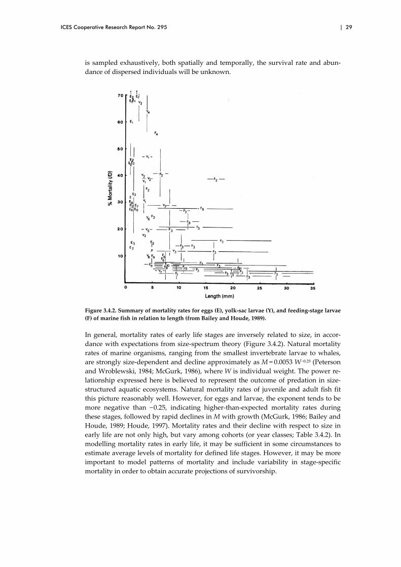
ICES Cooperative Research Report No. 295 | 29
is sampled exhaustively, both spatially and temporally, the survival rate and abun‐dance of dispersed individuals will be unknown.
Figure 3.4.2. Summary of mortality rates for eggs (E), yolk‐sac larvae (Y), and feeding‐stage larvae (F) of marine fish in relation to length (from Bailey and Houde, 1989).
In general, mortality rates of early life stages are inversely related to size, in accor‐dance with expectations from size‐spectrum theory (Figure 3.4.2). Natural mortality rates of marine organisms, ranging from the smallest invertebrate larvae to whales, are strongly size‐dependent and decline approximately as M = 0.0053 W −0.25 (Peterson and Wroblewski, 1984; McGurk, 1986), where W is individual weight. The power re‐lationship expressed here is believed to represent the outcome of predation in size‐structured aquatic ecosystems. Natural mortality rates of juvenile and adult fish fit this picture reasonably well. However, for eggs and larvae, the exponent tends to be more negative than − 0.25, indicating higher‐than‐expected mortality rates during these stages, followed by rapid declines in M with growth (McGurk, 1986; Bailey and Houde, 1989; Houde, 1997). Mortality rates and their decline with respect to size in early life are not only high, but vary among cohorts (or year classes; Table 3.4.2). In modelling mortality rates in early life, it may be sufficient in some circumstances to estimate average levels of mortality for defined life stages. However, it may be more important to model patterns of mortality and include variability in stage‐specific mortality in order to obtain accurate projections of survivorship.
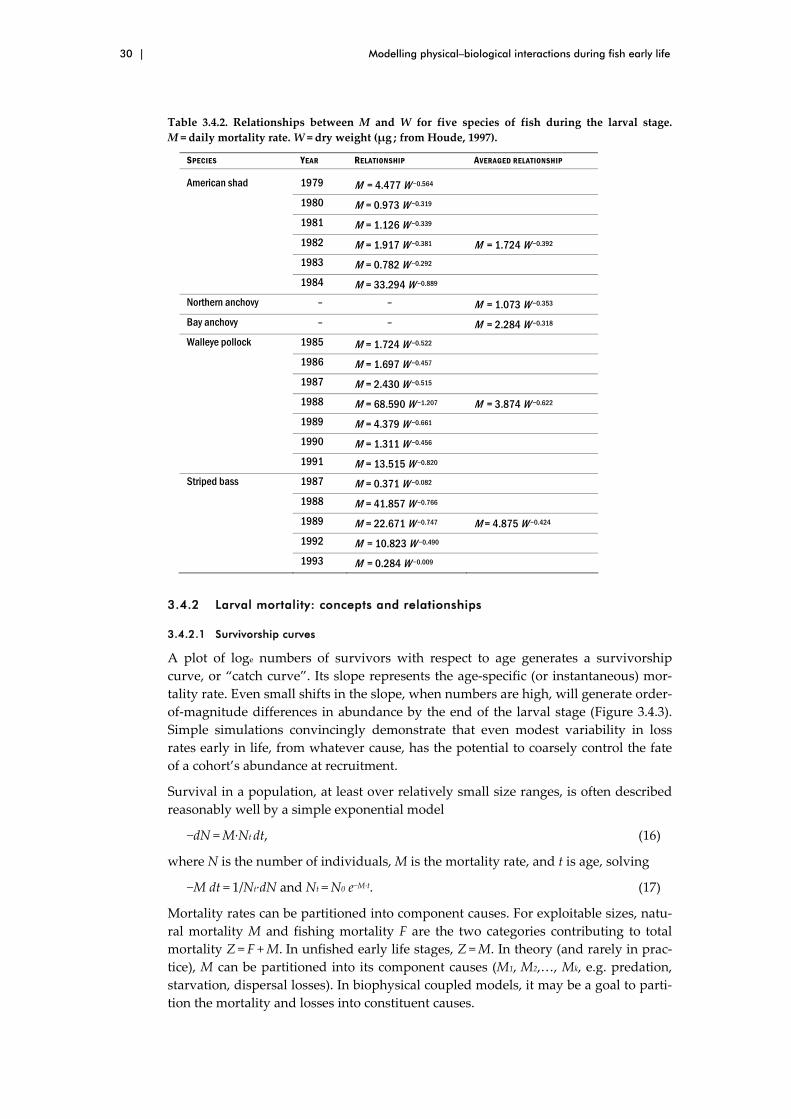
30 | Modelling physical–biological interactions during fish early life
Table 3.4.2. Relationships between M and W for five species of fish during the larval stage. M = daily mortality rate. W = dry weight (μg ; from Houde, 1997).
SPECIES YEAR RELATIONSHIP AVERAGED RELATIONSHIP
American shad 1979 M = 4.477 W −0.564
1980 M = 0.973 W −0.319
1981 M = 1.126 W −0.339
1982 M = 1.917 W −0.381 M = 1.724 W −0.392
1983 M = 0.782 W −0.292
1984 M = 33.294 W −0.889
Northern anchovy – – M = 1.073 W −0.353
Bay anchovy – – M = 2.284 W −0.318
Walleye pollock 1985 M = 1.724 W −0.522
1986 M = 1.697 W −0.457
1987 M = 2.430 W −0.515
1988 M = 68.590 W −1.207 M = 3.874 W −0.622
1989 M = 4.379 W −0.661
1990 M = 1.311 W −0.456
1991 M = 13.515 W −0.820
Striped bass 1987 M = 0.371 W −0.082
1988 M = 41.857 W −0.766
1989 M = 22.671 W −0.747 M = 4.875 W −0.424
1992 M = 10.823 W −0.490
1993 M = 0.284 W −0.009
3.4.2 Larval mortality: concepts and relationships
3.4.2.1 Survivorship curves
A plot of loge numbers of survivors with respect to age generates a survivorship curve, or “catch curve”. Its slope represents the age‐specific (or instantaneous) mor‐tality rate. Even small shifts in the slope, when numbers are high, will generate order‐of‐magnitude differences in abundance by the end of the larval stage (Figure 3.4.3). Simple simulations convincingly demonstrate that even modest variability in loss rates early in life, from whatever cause, has the potential to coarsely control the fate of a cohort’s abundance at recruitment.
Survival in a population, at least over relatively small size ranges, is often described reasonably well by a simple exponential model
−dN = M∙Nt dt, (16)
where N is the number of individuals, M is the mortality rate, and t is age, solving
−M dt = 1/Nt∙dN and Nt = N0 e−M∙t. (17)
Mortality rates can be partitioned into component causes. For exploitable sizes, natu‐ral mortality M and fishing mortality F are the two categories contributing to total mortality Z = F + M. In unfished early life stages, Z = M. In theory (and rarely in prac‐tice), M can be partitioned into its component causes (M1, M2,…, Mk, e.g. predation, starvation, dispersal losses). In biophysical coupled models, it may be a goal to parti‐tion the mortality and losses into constituent causes.

ICES Cooperative Research Report No. 295 | 31
Figure 3.4.3. Survivorship curve, showing effects of different mortality rates during early life stages (from Houde, 2002).
Mortality rates decline with size and age during early life. Initially, rates may be very high, exceeding 50 % d−1 in some species and commonly exceeding 10 % d−1 (Figure 3.4.1). In a review of estimates, the mean mortality rate (temperature‐adjusted) for larval stages of marine fish was M = 0.24, that is, 21.3 % d−1 loss (Houde and Zastrow, 1993). The mean M for freshwater fish larvae is somewhat lower, on average M = 0.16, that is, 14.8 % d−1. The greater mortality rate for marine larvae is probably a conse‐quence of their much smaller average size (Houde, 1994) and higher vulnerability to a more diverse community of predators. The average rates for the larval stage do not represent the pattern of decline in M that generally occurs as larvae grow. For marine species dying at the mean rate > 99.95 %, mortality occurs during the mean larval stage duration (D = 36 d). For “average” freshwater fish larvae, cumulative mortality is lower, but 96.4 % are expected to die in the D = 20.7 d mean larval‐stage duration.
3.4.2.2 Temperature effects
In broad, cross‐taxa analyses, mortality rates of early life stages scale directly with temperature. Species developing in low latitudes, or at seasonally high temperatures, suffer high mortality rates, whereas species from cold environments suffer lower mortality rates. Houde (1989) and Pepin (1991) quantified the relationships for larval stages. Mortality rates (at the ecosystem level, across taxa) increase at approximately 0.01 per degree C. For 26 marine species, Houde and Zastrow (1993) derived the rela‐tionship
M = 0.0149 + 0.0129T sb = 0.0029 r 2 = 0.46, (18)
where T represents temperature and sb represents the standard error of the regression coefficient. This relationship may be useful in exploratory modelling if estimates of M for a species are unavailable.
Across taxa, mortality and growth rates of marine fish larvae are strongly coupled during early life. Species suffering high mortality rates also have high growth rates, and both rates are strongly and positively correlated with temperature (Figure 3.4.4). Species from temperate and high latitudes die and grow at slower rates than species spawning in tropical habitats or under seasonally warm conditions. For weight‐specific growth of marine fish larvae (across ecosystems and taxa), the relationship with temperature is (Houde and Zastrow, 1993)
G = 0.0230 + 0.0106T sb = 0.0016 r 2 = 0.35. (19)
Lacking other knowledge, a first‐cut (and coarse) estimate of mortality could be de‐rived from the respective M and G ecosystem‐level estimators with respect to tem‐

32 | Modelling physical–biological interactions during fish early life
perature. Furthermore, estimates of growth rates are more often available than mor‐tality rates for larval fish. If an estimate of G is available at known temperatures, then a crude, first‐cut estimate of larval‐stage M is
M = 1.2170G – 0.0131. (20)
Despite differences in stage durations and daily rates of mortality and growth for species from warm or cold environments, their cumulative or stage‐specific mortali‐ties are similar because of the strong concordance between mortality and growth rates. That knowledge can be used to crudely parameterize models and derive esti‐mates of M. For example, species such as cod (Gadus morhua) and haddock (Melanogrammus aeglefinus), which spawn at temperatures < 10° C, spend approxi‐mately 100 d in the larval stage, whereas tropical species, such as the damselfish (Po‐macentridae), spawn at temperatures > 25° C and spend only 25 d in the larval stage. Yet, average survival at the end of their respective larval stages is similar because M and G are strongly correlated and increase at approximately the same rate with re‐spect to temperature (Figure 3.4.4).
G
M
D
0
0.05
0.1
0.15
0.2
0.25
0.3
0.35
0.4
0 10 20 30 40
Temperature (oC)
M o
r G (d
-1)
0
20
40
60
80
100
120
140
D (d
)
M=0.0129T+0.0149Sb=0.0029
G=0.0106T-0.0230Sb= 0.0016
D=515.94T-0.9213
Sb=0.1057
M
G
D
Figure 3.4.4. Effects of temperature on weight‐specific growth (G), mortality (M), and larval stage duration (D) for marine fish larvae. Averaged results for a combined taxa analysis (based on data from Houde and Zastrow, 1993).
3.4.2.3 Size effects
Although mortality rates decline as development and growth of larvae occur, the rate of decline with respect to body size or age varies among species and among cohorts (or year classes). For five species, the average relationships describing declines in M with respect to weight (W) during the larval stage (Table 3.4.2) ranged from W −0.318 to W −0.622. Relationships for clupeoid species (e.g. American shad, Alosa sapidissima, W −0.392; northern anchovy, Engraulis mordax, W −0.353; bay anchovy Anchoa mitchilli, W −0.318) had less negative exponents than perciform (striped bass, Morone saxatilis, W −0.424) or gadid (walleye pollock, Theragra chalcogramma, W−0.622) larvae. In all cases analysed (Houde, 1997), declines in M were more rapid than the W −0.25 predicted from allometric‐scaling and size‐spectrum theory. As an example of declines in mortality with respect to size, the averaged, estimated declines in M for walleye pollock (T. chalcogramma) for seven years were: 5 days old (5.8 mm, 95 μg dry wt), M = 0.23; 15 days old (8.5 mm, 400 μg dry wt), M = 0.09; 26 days old (12.2 mm, 1600 μg dry wt), M = 0.04. The mortality rates and patterns of declines in M during the larval stage can differ among cohorts and interannually in response to variable oceanographic condi‐tions and predation that larvae encounter. Because even relatively small changes in stage‐specific mortality rates can generate major variability in abundance of survi‐

ICES Cooperative Research Report No. 295 | 33
vors, only coarse estimates of survival can be obtained by parameterizing models with averaged relationships and rates. These may still serve a useful purpose to ini‐tialize modelling and gauge sensitivity in model output to variability in stage‐specific mortality rates.
3.4.2.4 Stage-specific mortality and estimates of abundance
When mortality is size‐ or stage‐specific, it may be desirable to estimate stage‐specific mortality and survival rates for early life stages. These rates can be derived from es‐timates of M and G and weights (W) at stages. The ratio M/G, sometimes referred to as the “physiological mortality rate” (Beyer, 1989; Houde, 1997), can be applied to define mortality within a stage(s)
Ms = (M/G)∙loge[Ws / Ws‐1], (21)
and survival rate is
Ss = Ns / Ns‐1 = e‐Ms = [Ws / Ws‐1] −M/G. (22)
When abundance‐at‐stages (or sizes) is determined and growth rates can be esti‐mated, M can be derived from this relationship. Estimates of Ms range widely, differ‐ing among species and interannually in response to particular life history and ontogenic patterns, and to environmental effects (e.g. temperature; Houde, 1997).
The M/G index is useful for interpretation of cohort dynamics: when its value is > 1, cohort biomass (B) is declining; when its value is < 1, B is increasing. M/G tends to be > 1 for most marine fish in the earliest larval stages. Relative, stage‐specific cohort biomass (Bs) and its trends during the growth of larvae can be derived as
Bs / Bs‐1 = [Ws / Ws‐1](1 – [M/G]). (23)
The among‐cohort or year‐class variability in size and age at which early life stages transition from M/G > 1 to < 1 describes variability in size‐specific survival patterns and may be of use in distinguishing successful from unsuccessful cohorts (successful cohorts making the transition at small size and young age).
3.4.2.5 Size-selective and growth-rate-selective mortality
Compensation and density dependence. A significant fraction of mortality in early life may be density‐dependent and can be modelled based on assumptions (or obser‐vations) of effects of prey limitation on growth (e.g. see Shepherd and Cushing, 1980). Small density‐dependent regulations of either G or M can generate substantial vari‐ability in survivor abundance and act to regulate recruitment levels. In practice, few estimates of the density‐dependent component of mortality in early life are available.
To estimate density‐dependent mortality, pairwise plots of log10 abundance estimates for cohorts sampled at two or more early life stages can be plotted (e.g. log10 Nt+1 plot‐ted on log10 Nt) and the slope of the resulting relationship estimated; if < 1.0, there is evidence of density‐dependent mortality, and its magnitude can be estimated from the regression statistics (Myers and Cadigan, 1993). Alternatively, the presence and magnitude of density‐dependent mortality can be estimated from the regression rela‐tionship between estimates of cumulative mortality in early life (MA) and initial abundance (A) of cohorts or year classes of eggs or larvae. A significant regression slope in this relationship indicates that density‐dependent mortality occurs. The y‐intercept of the regression (M0) is an estimate of the average density‐independent component of cumulative mortality (Savoy and Crecco, 1988). Estimates of the degree of density‐dependence for any initial level of abundance for cohorts or year classes

34 | Modelling physical–biological interactions during fish early life
can be derived from the regression (MA − M0). These approaches may be useful in pa‐rameterizing models for early life stages of species where annual or cohort‐specific estimates of abundance‐at‐stage or estimates of M are available.
Estimating larval mortality. Successful estimation of mortality depends on accurate determination of abundance and dependable assignment of individuals to age classes or stages. The general pattern of survivorship curves in early life is known (Figures 3.4.1 and 3.4.5). The difficulty and cost of estimating mortality of eggs and larvae are greatest in large ecosystems, which essentially may be unbounded and subject to sig‐nificant losses through dispersal and translocation, in addition to mortality losses. The possibility of success increases in embayments, estuaries, and freshwater habitats that are bounded and where dispersal losses are minor or are of little consequence if the entire system is sampled.
Age‐specific losses are often estimated from a “catch curve”, in which abundance‐at‐age of survivors is plotted on age (Figure 3.4.5). A log‐linear regression equation of loge abundance on age (stage) estimates the instantaneous mortality rate:
loge Nt = loge N0 – M∙t, (24)
where Nt is abundance at age t (usually days for early life stages), N0 is estimated abundance at the beginning of the stage, and the regression coefficient M estimates the instantaneous mortality rate. Cumulative mortality is M∙t and the survival rate is S = e −M∙t. In practice, catch curves are best fitted to stages with relatively short dura‐tions (age intervals) to minimize errors in M associated with its decline during growth.
A hypothetical survivorship curve (Figure 3.4.1) and tabulated summary (Table 3.4.1) illustrate a survivorship analysis based on catch curves for three prerecruit stages and a post‐recruit stage of a typical marine fish (parameter estimates resemble those of walleye pollock, T. chalcogramma). At youngest ages and smallest sizes, mortality rates are highest, often > 10 % d ‐1. They generally decline during growth and ontog‐eny. Cumulative mortalities (M∙t) are high during the egg‐larval (high M, short dura‐tion) and juvenile stages (low M, long duration) when > 99.5 % of individuals may perish.
Modelling mortality when rates are declining during early life may be best accom‐plished with a model other than the log‐linear catch curve. For example, the Pareto model assumes that mortality is a power function of age (or size):
loge Nt = loge N0 + β∙tα, (25)
where the coefficient β estimates the overall rate of decline and α is the shape pa‐rameter. This model may be particularly effective in estimating mortality when the decrease in mortality is particularly steep between the earliest life stages (e.g. eggs or yolk‐sac larvae) and later stages (Figure 3.4.5).

ICES Cooperative Research Report No. 295 | 35
Age (Days)
Log e
Abu
ndan
cePareto ModelLoge Nt = 21.435 - 2.563 *Age0.402
r2 = 0.93Exponential ModelLoge Nt = 17.514 - 0.206 *Ager2 = 0.86
Figure 3.4.5. Survivorship curve (catch curve) for early life stages of striped bass, Morone saxa‐tilis. Results of two model fits are included: exponential model (r 2 = 0.86) and Pareto model (r 2 = 0.93). Data point at day 0 represents egg abundance; remainder of data are for larvae (from Houde and Secor, 1996; unpublished report).
3.4.3 Causes of early-life mortality
3.4.3.1 Starvation and nutritional deficiencies (and critical periods)
Larval fish may die from starvation or other nutrition‐related causes. Estimating or modelling this component of mortality may be important. Direct estimates are diffi‐cult to obtain because poorly nourished larvae weaken, become increasingly vulner‐able to predation, and therefore occur less frequently than expected in ichthyoplankton collections. Selective predation on slower growing but healthy indi‐viduals may also occur, a mortality process potentially independent of larval nutri‐tional condition, but still nutrition related. Back‐calculation procedures, based on otolith microstructure analysis of early life stages sampled in two or more periods, can document and quantify relative losses to mortality of slow‐ and fast‐growing lar‐vae in a population, allowing estimates of growth‐related mortality to be made.
Critical periods (sensu Hjort) are observed infrequently in the sea. High mortalities of larvae at the time of first feeding, resulting in order‐of‐magnitude losses to the popu‐lation and concentrated in period of a few days, signify a critical period. Critical peri‐ods certainly can be evaluated in field research and simulated/parameterized in models.
3.4.3.2 Predation
Predators are probably the biggest single cause of mortality to early life stages of fish. Explicitly estimating the component of mortality attributable to predation is difficult. Predation losses may be linked to nutritional deficiencies that increase vulnerability of young fish to predators. Predation on fish eggs is size‐specific, and predation on larvae may be both size‐specific and growth‐rate‐dependent. As larvae grow and de‐velop, becoming less vulnerable to predators, mortality rates attributable to predation decline. Despite a wealth of laboratory research evaluating predation on fish eggs and larvae, and a proliferation of models on the predation process, predation remains difficult to detect or evaluate in the sea. Eggs and especially larvae are soft‐bodied

36 | Modelling physical–biological interactions during fish early life
and are destroyed upon consumption or are digested quickly. As a consequence, eggs and larvae may go undetected or be underrepresented as prey in predator guts.
Important predators of fish eggs and larvae include juvenile and adult fish, jellyfish (ctenophores and medusae), chaetognaths, and euphausiids. There is a general lack of information on the community of predators consuming fish eggs and larvae, espe‐cially in quantifying mortality attributable to specific predators, making it difficult to evaluate predator taxa and the taxon‐specific mortality imposed on eggs and larvae. Research to date, including modelling approaches, has rarely succeeded in convinc‐ingly partitioning mortality of young stages of fish among the array of predator taxa and sizes present in the sea.
Vulnerability of larval fish to types of predators can be modelled and illustrated prin‐cipally by dome‐shaped curves in relation to larval size (see Figure 9 in Bailey and Houde, 1989). The susceptibility of larvae to attack and capture by a particular type and size of predator generally declines as larvae grow, being a function of increases in swimming speeds, improved ability to detect predators, and better avoidance and escape capability. Vulnerability, representing the net effect of ontogenetic changes in encounter probability and susceptibility, may increase for intermediate‐sized larvae, at least for a particular predator of specific size and capability. With continued growth, fish larvae become increasingly adept at avoiding predation, thus reducing their vulnerability, despite the increased probability of encounter. Through growth, larvae also eventually reach sizes that reduce their vulnerability to gape‐limited predators.
Laboratory experiments have demonstrated the size‐specific nature of predation. Predators, independent of taxon, tend to consume larval fish prey that, on average, are about 10 % of the predator’s body size (Paradis et al., 1996); this is a useful value for exploratory modelling applications. Perhaps surprisingly, Paradis et al. (1996) found that the 10 % value applied to both invertebrate and vertebrate predators.
Mortality from cannibalism on pelagic eggs is common in some clupeoid fish, either by incidental filter‐feeding or by selective consumption. A significant fraction of egg and yolk‐sac larval mortality (e.g. 20 %) in sardines (Sardinops spp.) and anchovies (Engraulis spp.) in upwelling ecosystems can be accounted for by egg cannibalism. Cannibalism may also occur when metamorphosing larvae settle onto substrate al‐ready occupied by older and larger conspecifics. Sibling cannibalism, in which larvae prey upon siblings, is reported in many taxa, including freshwater characids and ma‐rine scombrids.
3.4.3.3 Physics: transport, retention, and dispersal
Losses of early life stages to dispersal must be accounted for in coupled biophysical models. If eggs and larvae were passive particles, estimation of dispersal losses would be fairly straightforward. Behaviour of larvae, especially vertical migratory behaviour, in a stratified ocean adds complexity to estimating the loss term from dis‐persal. Dispersal losses may be a component of mortality if eggs or larvae cannot survive in environments where they are dispersed or cannot return to juvenile nurs‐eries. Fine‐scale variability in water‐column properties, especially stratification and its relationship with vertical distributions of fish eggs and larvae, their predators, and prey, plays a critical role in controlling conditions that determine retention or disper‐sal of early life stages and their potential for survival.
Dispersal losses are generally higher in smaller (or partly sampled) ecosystems than in larger ecosystems. Helbig and Pepin (1998b) defined methods useful for providing

ICES Cooperative Research Report No. 295 | 37
coarse estimates of advective losses as a function of ecosystem size. Their approach and results may be useful in parameterizing models that explicitly attempt to esti‐mate mortality and advective losses (see Figure 1 in Helbig and Pepin, 1998b). Helbig and Pepin (1998b) defined relationships for apparent mortality rate (Mt) and advec‐tive losses (Md) with respect to size of the sampled ecosystem based on several stud‐ies, from which they then derived estimates of actual mortality (M):
M = Mt – Md. (26)
Although it is clear that physics at meso‐ and broader scales (from one to hundreds of kilometres) plays a role in controlling levels of mortality of larval stages, physics at finer scales (e.g. on millimetre to metre scales) can also be important. It is these spa‐tial scales that determine contact rates between young fish, their prey, and predators. Rates of contact, controlled by micro‐scale turbulence, for example, can directly influ‐ence the nutritional status of larvae and indirectly affect their vulnerability to preda‐tion. Modelling research, laboratory experiments, and some field observations on the role of micro‐turbulence in promoting larval feeding success, growth, and survival have helped to explain how high survival of fish larvae in the sea is possible under conditions where average prey levels apparently are lower than required for larval survival. For Atlantic cod larvae (and by inference, other species), it is apparent that survival is maximized under moderate wind conditions, which generate micro‐turbulence sufficient to enhance encounter rates between larvae and prey, but not so turbulent that larvae are unable to capture prey (MacKenzie and Kiørboe, 2000).
3.4.3.4 Water quality and habitats
Contaminants and toxic materials, acting either chronically or episodically, can be lethal to eggs and larvae of fish, or may prevent successful spawning by adults. This is probably most important in small ecosystems, such as bays and estuaries, and for populations quasi‐restricted to these areas. Other water‐quality factors may act indi‐rectly or interactively. For example, increased loadings of nutrient, such as nitrogen and phosphorus, can lead to eutrophication of many fresh waters, estuaries, and coastal ecosystems, which can deplete dissolved oxygen, leading to hypoxia or anoxia that is lethal to fish eggs and larvae. In another example, effects of contaminants or poor water quality may alter behaviour of larvae, so impeding feeding and reducing growth rates, or making larvae more vulnerable to predation.
3.4.3.5 Diseases and parasites
Except in aquaculture, we seldom consider or estimate mortality of fish eggs and lar‐vae from diseases or parasites, although these sources of mortality may be important. Parasites of eggs and larvae, including dinoflagellates, protozoans, helminths, and copepods, have been reported regularly, although mortality rates and population‐level consequences are unevaluated. In the sea, diseased, parasitized, and poorly conditioned larvae and eggs disappear rapidly from populations either through se‐lective predation or through decomposition and settlement of dead bodies.
3.4.3.6 Interacting factors
In many circumstances, it is a simplification to assign conditional probabilities to sources of mortality without understanding potential interactions. For example, the fraction of young stages dying from starvation or predation cannot be easily parti‐tioned because the two sources of mortality interact. Poorly fed, slow‐growing larvae are more vulnerable to predators. In laboratory experiments and model simulations, such larvae are selectively predated and have a relatively low probability of survival.

38 | Modelling physical–biological interactions during fish early life
In the sea, it remains problematic to quantify the fractional mortalities on larval fish from either starvation or predation. Low prey levels reduce growth rates, leading to longer stage durations during early life and a greater probability of being predated. Modelling experiments (IBMs) have demonstrated how growth rate and its variabil‐ity can modify effects of predation on survival of larval fish (Rice et al., 1993; Cowan et al., 1996; Letcher et al., 1996). High growth rates, and also variable growth rates, lower the overall expectation of mortality in a larval population vulnerable to size‐selective predation.
Parameterizing models to depict accurate mortality requires consideration of the in‐teractions among the physical and biological processes affecting survival. In many cases, failed retention, unfavourable transport, or poor environmental conditions (e.g. temperature, pH, hypoxia) act directly to kill some fraction of eggs and larvae, but these same conditions will also affect the predators and prey of early life stages, creat‐ing a complex web of interactions affecting early life survival. Cascading effects can increase the mortality risk to eggs and larvae in stressed ecosystems. For example, an excess of nutrients can promote eutrophication, leading to low dissolved oxygen, harmful algal blooms, losses of aquatic vegetation, and probable increases in some larval predators (e.g. jellyfish), as the trophic state of an ecosystem shifts. Evaluating the effects of such multiple, complex sources on early‐life mortality is difficult and seldom achieved, except in modelling, where simulations may provide valuable in‐sight into these interacting processes.
3.4.4 Case study: mortality and the super-individual concept
A major problem in an individual‐based model, once mortality is included, is that extraordinarily large numbers of individuals are needed at the start of a simulation if they are to be continually eliminated by a mortality function during the course of the simulation. Obviously, this procedure results in prohibitive computational times and may cause storage problems. Additionally, this common solution, that is, the contin‐ual reduction of the number of individuals in the model, can lead to loss of variation, irregular dynamics, and a large sensitivity to the value of the random generator seeds introduced at the start (Scheffer et al., 1995). The super‐individual concept developed by Scheffer et al. (1995) is ideally suited to eliminate, or rather circumvent, these prob‐lems. The solution is to add an extra variable to each model individual, namely the number of individuals it actually represents. In essence, each particle is considered as a super‐individual representing a specific number of eggs at the outset of the simula‐tion, with this number declining according to the mortality function applied during the course of the simulation. Thus, the resulting super‐individuals are, in fact, classes of individuals (Scheffer et al., 1995).
To elucidate the incorporation of mortality in individual‐based models (IBMs) using the super‐individual concept, an example of a mackerel IBM is presented below, which has been successfully used to predict the survival of mackerel post‐larval stages in the Northeast Atlantic (Bartsch and Coombs, 2004; Bartsch et al., 2004; Bartsch, 2005). This IBM is composed of a number of physical and biological modules to simulate transport, growth, and mortality. It is an i‐space configuration model (DeAngelis and Rose, 1992) in which large numbers of individuals are followed as discrete entities. As the parameterization of mortality in this IBM is based on daily absolute growth rates, a brief description of the growth module is given for the sake of both clarity and completeness.
ICES Cooperative Research Report No. 295 | 39
3.4.4.1 Growth module
In the growth module, the growth rates of larvae and post‐larvae are calculated daily as a function of temperature, length, and ambient food concentration. In the absence of sufficient detailed information on the changing spatial and seasonal vertical distri‐bution of food particles, the food‐concentration data are specified as being vertically homogeneous within the entire depth range of the larvae and post‐larvae (the upper 60 m of the water column). The data were computed as weekly fields for the model area for the period from mid‐January to mid‐September for each of the years 1998, 1999, and 2000.
Food concentrations were modelled from egg‐production rates of representative large (Calanus) and small (Acartia) copepods, these constituting 39 – 58 % of the diet of larval and post‐larval mackerel (Hillgruber et al., 1997; Conway et al., 1999; Hillgruber and Kloppmann, 2001; SEAMAR, 2002). Based on the formulations given in Prestidge et al. (1995), the egg‐production rates were calculated based on the input variables of satellite‐derived sea surface temperature (SST) and chlorophyll a concentration, pro‐viding monthly fields interpolated to weekly averages for each year. Egg‐production rates per female were raised to population‐production rates using Continuous Plank‐ton Recorder data (Sir Alistair Hardy Foundation for Ocean Science, Plymouth, UK) and SEAMAR field sampling data on sex ratio and relative abundance of copepodite stages. Finally, production was converted to biomass using published copepod demographics and raised proportionately to total biomass based on the observed fraction of plankton dry weight represented by Calanus and Acartia. A full description of the food availability model is given in SEAMAR (2002).
A first analysis of growth from field data sampled on cruises during 1999 demon‐strated that a logistic curve was an appropriate approximation of mackerel larval and early post‐larval growth (SEAMAR, 2002), using a variable exponential parameter r (Bartsch, 2002):
L = L∞(1 + exp(−rt+c))−1, (27)
where L is the length in mm at time t, L∞ is a constant representing the maximum length attainable in the initial larval and early post‐larval growth stanza (set at 80 mm), r is a function of temperature and food concentration (see below), c is the constant of integration, and L = 3 mm at time t = 0, that is, at hatch.
The absolute growth rate is a function of length and the exponential parameter r:
dL/dt = G = rL(1 – (L / L∞)). (28)
Temperature and food mediation of the parameter r is carried out as follows:
r = (ropt – d(Topt – T)2)Fi (29)
where ropt is the maximum specific growth rate (ropt = 0.125), d is a constant (d = 0.00085), Topt is the optimum temperature for growth (19° C), T is the temperature encountered, and Fi is a model food index (MFI: see below).
The range of appropriate values for ropt and d depends mainly on the seasonal tem‐perature range and growth rates. Using the available field data, values for the pa‐rameters ropt and d were determined in order to provide realistic values of r, that is, r must remain positive and should tend to some minimum value rmin (Bartsch, 2002) that corresponds to the lowest growth rates observed in the field when substituted into Equation (28). The temperature optimum for growth (Topt = 19° C) was selected on the basis of the field temperatures likely to be encountered by larval and post‐larval

40 | Modelling physical–biological interactions during fish early life
mackerel (maximum of ca. 20° C) and the general energetic consideration that, within the normal ecological range of a species, higher temperatures lead to increased growth rates (see e.g. Otterlei et al. (1999) for optimum growth temperature for larval cod, Gadus morhua).
The first stage in setting the MFI in Equation (29) is calculation of the ratio of avail‐able food to the required daily ration for a particular sized larva or post‐larva. This is based on a simple energetics model (SEAMAR, 2002) of weight‐based daily growth rate, body length, food concentration, light level, and food capture efficiency. The numerical value of the ratio varies between 0.00001 and >> 1. Values > 1 are set to unity, because these values denote maximum growth in optimum food concentra‐tions (i.e. food concentrations above which no further food assimilation can be achieved). For use in Equation (29), the range of ratio values was linearly rescaled to give an MFI with a range of 0.4 – 1.0. The lower boundary for the MFI was determined from sensitivity tests, such that growth rates from Equation (28), using r from Equa‐tion (29) and substituting MFI = 0.4, were not lower than observed in the field during SEAMAR. A full description of the parameterization of the food and growth relation‐ship is given in SEAMAR (2002).
For each super‐individual in each grid box, the calculated MFI is modified by a ran‐dom ∆MFI to mimic subgrid variations in food concentration, which are not resolved by the model grid. These random ∆MFI are drawn from a top‐hat distribution of width 0.2, which results in a maximum deviation of ± 0.1 from the calculated MFI for a super‐individual d−1. Values calculated at < 0.4 were set to 0.4. The choice of the numerical value for ∆MFI was based on the requirement to allow subgrid variation without modifying MFI significantly.
3.4.4.2 Mortality module
The daily mortality rates of the super‐individuals are calculated as a function of length and absolute growth rates. This determines the daily decrease in numbers of the original 106 individuals represented by each super‐individual in the mackerel IBM. Conceptually, each super‐individual can be considered a subset of a cohort. On any day D, ND,i is the number of eggs or larvae represented by each super‐individual and is termed the number of “virtual individuals”. In essence, ND,i is different for each particle, because egg‐development time is temperature‐dependent, growth is temperature‐ and food‐dependent, and mortality depends on absolute growth rates and length, and so implicitly dependent on temperature and food concentration.
The mathematical relationships between growth and mortality have been examined in a number of papers, those of most significance to the present formulation being Anderson (1988), Miller et al. (1988), Beyer (1989), Morse (1989), Houde (1989, 1997), and Pepin (1991, 1993). The conclusion is that growth can be used to represent rela‐tive survival, because length‐specific growth rates and mortality interact to determine survival of a cohort during the prerecruit period. Mortality considered here is caused by both starvation and predation. Based on this, mortality was formulated such that:
• Absolute growth rates and mortality rates are positively correlated; • Mortality rates are inversely correlated with larval length, that is, mortality
decreases as length increases; • Cumulative mortality within a specific length range decreases with in‐
creasing length.
The mathematical relationship linking mortality with growth rates and length in the mackerel IBM was based on an empirical relationship given by Pepin (1991):

ICES Cooperative Research Report No. 295 | 41
M = 5.17G 0.74L−1.17, (30)
where G is the absolute growth rate in mm d−1 and L is length in mm. The empirical formulation given above is principally similar to an equation of the form
M = cG1−x/L1+x, (31)
where c is a constant.
Using daily data over a length range of 3 – 80 mm from the logistic curve for G and L (Equations (27) and (28)), a range of sensitivity tests were carried out to find an ap‐propriate value for x in Equation (32) below that would satisfy the above three crite‐ria. These results demonstrated that x should be ≥ 0.3. A numerical value of x = 0.3 was selected, because this provided exponential values for G and L that were suffi‐cient for meeting the criteria and closest to their exponential values in Equation (30). Thus, the final formulation for the daily mortality rate in the mackerel IBM was
M = 5.0G 0.7/L 1.3. (32)
The super‐individual concept used in the deterministic mackerel IBM described above has the following advantages over IBMs that do not use this concept.
• There is no need for extraordinarily large numbers of particles at the be‐ginning of the simulation.
• Computational time is drastically reduced. • There is no need to remove specific particles from the simulation, that is,
the problem of reseeding does not arise.
The mathematical formulation described here to parameterize larval mackerel mor‐tality yields higher growth rates at higher temperatures and, hence, higher daily mor‐tality rates, but the stage‐specific mortality rates are lower for fast‐growing individuals, that is, they move faster through (not only) vulnerable stages.
Generally, larval mackerel mortality rates in the IBM usually start off at about 30 – 40 % d−1 and drop below 10 % d−1 after about 35 – 45 d. However, it should be noted that these values vary widely between separate individuals because mortality de‐pends on temperature and food concentration, which are both spatially and tempo‐rally variable. This results in a wide range of surviving virtual individuals per super‐individual and, hence, a marked inhomogeneous distribution of model survivors over the whole model area (Bartsch et al., 2004). This is demonstrated in Figure 3.4.6.

42 | Modelling physical–biological interactions during fish early life
Figure 3.4.6. (a) Initial particle (egg) distribution for 12 March – 3 June, as used in all model runs; (b) regional distribution of the total remaining virtual individuals within each model grid box at a length of 50 mm for 1998; (c) for 1999; and (d) for 2000.
3.5 Behaviour and settlement
Jean‐Olivier Irisson, Jeffrey M. Leis, Claire B. Paris, and Howard I. Browman
3.5.1 Introduction
Fish larvae are not passive particles, and it is becoming increasingly obvious that they have behavioural capabilities that may greatly influence dispersal outcomes and other biophysical processes (Leis, 2006). Thus, the simplifying assumption of passive behaviour, which has been the basis for many biophysical models in the past, can no longer be justified as the default assumption (Leis, 2007). Behaviour as a potentially important factor that can influence the outcomes of such models must be considered as a real alternative. This requires an understanding of the behaviour of the larvae, something that is frequently lacking. Recent research has demonstrated that fish lar‐vae have behavioural capabilities in areas of swimming, orientation, and sensory abilities that were unknown and unexpected only ten years ago.
“Behaviour” refers to the actions or reactions of organisms, usually in relation to the environment. Larval behaviour can become overwhelmingly complex because indi‐viduals acquire behavioural capabilities as they develop. However, a “good” model should not try to be exhaustive, but only include observed behaviours that are suffi‐cient to reproduce patterns and/or mechanisms relevant to the scope of the study. Sensitivity analyses, in which different behaviours are added to the model to assess their influence on outcomes, can aid in determining which behaviours to incorporate.
In this section, we consider vertical positioning, horizontal swimming, orientation, foraging, predator avoidance, schooling, and settlement. All these behaviours can influence the outcome of the larval phase and may need to be considered when de‐

ICES Cooperative Research Report No. 295 | 43
signing a model. The following sections provide clues on whether or not it is worth implementing each behaviour, depending on the a priori knowledge of the system and the other processes already included in the model. Each is organized in a similar fashion: (i) outlining how the behaviours can be important to the processes that the model seeks to address, (ii) proposing simple tests on how to determine whether or not it has any influence, (iii) giving insights on how to obtain relevant data and point‐ing to appropriate literature references, and (iv) suggesting implementations for this behaviour in a model.
We further encourage modellers to test the relative influence of separated physical conditions and behaviour for their particular model/species/area of interest. Sensitiv‐ity analysis of model output to behaviour‐related parameters or functions should be done routinely after each behaviour is implemented, as well as comparison of predic‐tions with empirical data. The following sections are intended to help the reader an‐swer the question, what are the priorities for implementation of different behaviours?
3.5.2 General questions on behaviour-related traits
3.5.2.1 Mean vs. mean + variance vs. maximum
All behavioural traits are variable: swimming speeds and vertical position change among and between individuals; sensitivity to environmental cues for orientation can similarly vary, as can response to these cues, etc. Therefore, the description of behav‐iour has to be probabilistic to account for these variations. Behavioural studies, whether they are experimental or done in the field, allow an estimate of population traits. The question then is, which population descriptors are most relevant to a model of the early life history of fish?
In such models, we are mostly interested in the individuals that survive the larval phase and recruit successfully. If most larvae succeeded, their mean behavioural traits, and those of the whole population, would be similar. Hence, including mean population traits in models could suffice to predict recruitment correctly. However, very few larvae survive the larval phase (see Section 3.4 Mortality; Doherty, 1983), and the few that do probably succeed because their traits are different from the others and well suited to the circumstances they encountered within the heterogeneous pe‐lagic environment (Fuiman and Cowan, 2003). For example, there is now evidence from several systems and species that the fastest growing individual larvae are most likely to survive, and the same may apply to behavioural performance. Therefore, using mean population performance in models will not be appropriate if the survi‐vors constitute only a small portion of the performance distribution. Variance around the mean has to be derived from observations (e.g. Browman et al., 2003) or estimated from published accounts and incorporated into the model to provide a realistic range of individual results. In addition, maximum values should also be considered be‐cause successful recruits may be the very few “best” individuals of each cohort. Comparison of model results based on both mean and best performance should be informative. Such a probabilistic approach can be accomplished through individual‐based models (IBMs), where traits of individual particles can be assigned following a probability density function.
3.5.2.2 Ontogeny of behaviour
Like morphology, behaviour develops during the pelagic larval stage from essentially planktonic at its start to nektonic at its end. The passive portion of the pelagic larval stage is likely to be short, and models that make the simplifying assumption are

44 | Modelling physical–biological interactions during fish early life
likely to be applicable to only a short portion of the larval stage. In addition to onto‐genetic changes in behavioural ability, there are often ontogenetic changes in the use of those abilities (e.g. age‐related changes in depth or in swimming direction). Meth‐ods for modelling behaviour need to be adjusted according to the state of knowledge of physical – biological interactions that result in larval growth. Indeed, most studies indicate that size (or stage of development) is a better predictor of behavioural ability than age (Fuiman and Higgs, 1997).
• When growth or development is explicitly included in the model (possibly via trophic interactions), behaviour can be formulated as a function of size or developmental stage. In addition, this relationship should consider not only the mean value for the population but also associated variation. In this case, as larvae are subjected to differential growth (e.g. in a model with heterogeneous spatially explicit resources), they will have differential performance of a given behaviour.
• When larval growth is not resolved in the model, or when not enough in‐formation is available to predict a continuous relationship between size and behavioural performance, milestones can be used to model behaviours in a simplified, stepwise manner. Morphological or ontogenetic stages can be expressed by a dimensionless metric, such as an ontogenetic index (Fuiman and Higgs, 1997) or developmental age (Job and Bellwood, 2000).
3.5.2.3 Taxonomic resolution of behaviour
Ideally, the behaviour of the larvae of the species to be modelled should be incorpo‐rated into the model. However, it is important to know the degree to which the be‐haviour of a particular species can be extrapolated to other taxa, because it is unlikely that we will ever have even partial information on the behaviour of all fish species. Currently, the amount of information available on any particular behaviour is limited to relatively few species and, for the vast majority of these, to only a portion of the larval stage (usually older larvae). When deciding whether or not behavioural infor‐mation from species A can justifiably be used in a model for species B, two things must be considered at the outset: (i) the closeness of the relationships of the two spe‐cies, and (ii) the similarity of the environment in which the species live.
The vast diversity of teleost fish species – approximately 27 000 species in 448 families divided among 40 orders (Nelson, 2006) – means that some species are very distantly related, with evolutionary histories that have been separate for tens of millions of years. Among orders in particular, there is no reason to assume that behaviours will be similar. Within mammals, for example, no one would assume that the behaviour of a tiger (Order Carnivora) would be similar to that of a dugong (Order Sirenia). Likewise, no one should assume that the behaviour of a plaice larva (Order Pleu‐ronectiformes) would be similar to a herring larva (Order Clupeiformes). As a gen‐eral rule of thumb, in the absence of other information, the closer the relationship between two species, the more justifiable it should be to assume they have equivalent behaviour. The use of well‐corroborated phylogenies that encompass the species un‐der consideration is essential in assessing the closeness of relationships, but such phylogenies do not exist for many fish taxa. Even this rule of thumb should be ap‐plied cautiously because there are many examples of larvae of confamilials with dif‐ferent behaviours. For example, in pomacentrids, the larvae of some species are found in midwater, whereas those of other species prefer the top few centimetres of the water column (Leis, 2004). Sibling species (e.g. Pacific herring and Atlantic her‐ring) are more likely to have similar behaviour than randomly chosen confamilials.
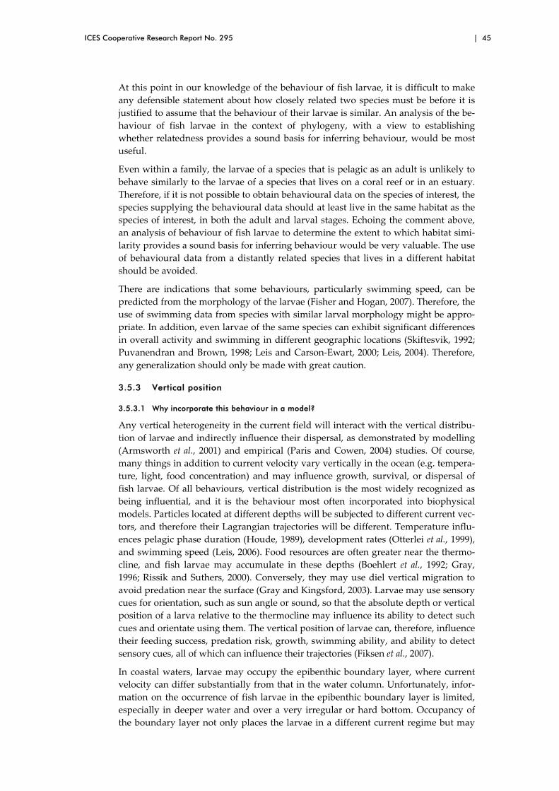
ICES Cooperative Research Report No. 295 | 45
At this point in our knowledge of the behaviour of fish larvae, it is difficult to make any defensible statement about how closely related two species must be before it is justified to assume that the behaviour of their larvae is similar. An analysis of the be‐haviour of fish larvae in the context of phylogeny, with a view to establishing whether relatedness provides a sound basis for inferring behaviour, would be most useful.
Even within a family, the larvae of a species that is pelagic as an adult is unlikely to behave similarly to the larvae of a species that lives on a coral reef or in an estuary. Therefore, if it is not possible to obtain behavioural data on the species of interest, the species supplying the behavioural data should at least live in the same habitat as the species of interest, in both the adult and larval stages. Echoing the comment above, an analysis of behaviour of fish larvae to determine the extent to which habitat simi‐larity provides a sound basis for inferring behaviour would be very valuable. The use of behavioural data from a distantly related species that lives in a different habitat should be avoided.
There are indications that some behaviours, particularly swimming speed, can be predicted from the morphology of the larvae (Fisher and Hogan, 2007). Therefore, the use of swimming data from species with similar larval morphology might be appro‐priate. In addition, even larvae of the same species can exhibit significant differences in overall activity and swimming in different geographic locations (Skiftesvik, 1992; Puvanendran and Brown, 1998; Leis and Carson‐Ewart, 2000; Leis, 2004). Therefore, any generalization should only be made with great caution.
3.5.3 Vertical position
3.5.3.1 Why incorporate this behaviour in a model?
Any vertical heterogeneity in the current field will interact with the vertical distribu‐tion of larvae and indirectly influence their dispersal, as demonstrated by modelling (Armsworth et al., 2001) and empirical (Paris and Cowen, 2004) studies. Of course, many things in addition to current velocity vary vertically in the ocean (e.g. tempera‐ture, light, food concentration) and may influence growth, survival, or dispersal of fish larvae. Of all behaviours, vertical distribution is the most widely recognized as being influential, and it is the behaviour most often incorporated into biophysical models. Particles located at different depths will be subjected to different current vec‐tors, and therefore their Lagrangian trajectories will be different. Temperature influ‐ences pelagic phase duration (Houde, 1989), development rates (Otterlei et al., 1999), and swimming speed (Leis, 2006). Food resources are often greater near the thermo‐cline, and fish larvae may accumulate in these depths (Boehlert et al., 1992; Gray, 1996; Rissik and Suthers, 2000). Conversely, they may use diel vertical migration to avoid predation near the surface (Gray and Kingsford, 2003). Larvae may use sensory cues for orientation, such as sun angle or sound, so that the absolute depth or vertical position of a larva relative to the thermocline may influence its ability to detect such cues and orientate using them. The vertical position of larvae can, therefore, influence their feeding success, predation risk, growth, swimming ability, and ability to detect sensory cues, all of which can influence their trajectories (Fiksen et al., 2007).
In coastal waters, larvae may occupy the epibenthic boundary layer, where current velocity can differ substantially from that in the water column. Unfortunately, infor‐mation on the occurrence of fish larvae in the epibenthic boundary layer is limited, especially in deeper water and over a very irregular or hard bottom. Occupancy of the boundary layer not only places the larvae in a different current regime but may

46 | Modelling physical–biological interactions during fish early life
also expose them to increased risk of predation from benthic predators and to in‐creased turbidity, and may place them in a different food regime. Similarly, some marine structures, such as kelp beds and reefs or other high‐relief bottom topogra‐phy, provide areas of flow that differ substantially from those in the far‐field water column; these should be taken into account if larvae occur near them.
3.5.3.2 How to determine whether or not this behaviour influences dispersal outcome
Current velocity, hydrography (e.g. salinity, temperature), and fluorometry profiles (or their modelled equivalents) over the estimated spatial scales and depth range of interest (i.e. observed larval fish depth range) are required to evaluate the degree of vertical shear in the current, temperature gradient, and depth of chlorophyll maxi‐mum. Larvae may use sensory cues for orientation, such as sun angle or sound ema‐nating from a settlement habitat, so the absolute depth or vertical position of a larva relative to the thermocline may influence their ability to detect such cues and orien‐tate using them. Clearly, if heterogeneity in the velocity field is detected, vertical dis‐tribution of larvae must be included in a model. If some model parameters or functions (such as survival, growth rate) explicitly depend on food availability or temperature, and if these are not homogeneous on the depth range of interest, verti‐cal position must be included. Finally, sensory cues must be included if they are known to be used by larvae for orientation and are also affected by the vertical struc‐ture of the water column. Some models integrate water movement over the surface Ekman Layer, but water velocity over this layer is known to differ with depth. This means that larvae at different depths within the Ekman Layer will be subject to dif‐ferent current speeds and directions, and this should be reflected in the model.
3.5.3.3 Simple tests
When a three‐dimensional oceanographic model is available, the influence of vertical migration can be assessed by comparing the fate of particles constrained to the top and bottom layers within the species’ depth range. When three‐dimensional oceano‐graphic models are computationally infeasible, then two‐dimensional models are of‐ten employed. If the model simulates horizontal (e.g. cross‐shelf) and vertical (e.g. depth) dimensions, then the influence of vertical position can be tested in a manner similar to that used for three‐dimensional models. If the model dimensions do not include the vertical, then there is no simple test for the potential influence of vertical migration in the model. If a strong vertical current shear is observed in the field and larvae are observed to migrate through it, then the use of a three‐dimensional model is recommended.
3.5.3.4 How to obtain the relevant data
Vertical distribution is probably the behaviour about which we have the most infor‐mation. It has been explored primarily with towed nets, performing stratified sam‐pling of the water column. This requires multisampling nets, preferably the Multi Opening and Closing Net and Environmental Sensing System (MOCNESS), or re‐peated single‐net (e.g. bongo net) sampling of the same area at different depths. To resolve diel vertical migration, a few stations should be sampled over several 24 h cycles. Similar information can be obtained from pump samples, but pumps suffer from significant avoidance, particularly when sampling larger larval stages. Nets also suffer from avoidance, and care must be taken when analysing ontogenetic vertical distribution data (e.g. gear selectivity can be calculated from the net opening, mesh size, and length – frequency distribution of the larvae caught).

ICES Cooperative Research Report No. 295 | 47
Acoustic methods can also provide useful information on vertical distribution, but suffer from difficulties in identifying the species whose vertical distribution they por‐tray. Finally, in situ observations of larvae by divers (Leis, 2004) can provide detailed information on vertical distribution and changes therein from the individual larvae that are caught, typically with light traps, and subsequently released. This approach is limited by diver‐safety considerations to relatively shallow depths and can only be used in the daytime and for larvae > ca. 5 mm.
This kind of sampling provides information about the concentration of larvae caught within specific depth intervals. Sampling can be carried out repeatedly along a single transect, generating two‐dimensional data, or over a spatial domain to obtain a three‐dimensional description of larval patches (e.g. Paris and Cowen, 2004). In order to describe the vertical distribution of the larval population, two‐dimensional sampling is adequate, and the resulting information needs to be summarized using statistical descriptors. Interesting descriptors are the depth centre of mass of the larval patch, its variance, the total depth range in which larvae are caught, and depth – frequency dis‐tribution. Each observation (i.e. depth interval) must be reduced to its mean depth. Raw larval counts should be converted to concentrations, using the volume sampled, and standardized using the depth range of the interval. Finally, mean depths should be weighted by these standardized concentrations to compute descriptive statistics of the vertical distribution of larvae: weighted mean depth (i.e. depth centre of mass), standard deviation, quantiles, etc. An alternative to a depth centre of mass portrayal of vertical distribution is a depth – frequency distribution. Depth bins, usually deter‐mined by the vertical resolution of the sampling design, are established, and the mean percentage (and associated variance) of the larval population in the sampled water column is calculated for each bin. This offers some advantages over the centre mass in terms of detail, but is less robust in respect to deviation from the sampling plan (e.g. different depth intervals between stations) and more difficult to transfer to a model.
In addition, these descriptive statistics should be discussed dynamically in time and ontogeny. For example, the differences between day and night conditions, or between several ontogenetic stages, should be investigated and described, if present.
Furthermore, the movement of individuals, and not only the distribution of the popu‐lation mean, is important. A simple example highlights this fact taken from Leis (2006).
Imagine a stratified system with a flow of x in an upper layer equal, but op‐posite, to that in a lower layer, and with the larvae equally distributed verti‐cally between the two layers. If there is no movement by individual larvae between layers, at the end of time t the larvae in the upper layer will be ad‐vected a horizontal distance of 2zt relative to those in the lower layer. If movement of larvae between layers is constant and individuals spend an equal amount of time in each layer, then the larvae in the two layers will not become horizontally separated at all. Depending on the proportion of time an individual spends in each layer, any other result intermediate between these extremes is possible.
This information can be obtained by in situ observations of larvae over time to deter‐mine their individual vertical movements (e.g. Leis, 2004) or by the use of specialized sampling equipment that can determine the upward and downward movement of individuals rather than vertical shifts of population means (e.g. Pearre, 1979).

48 | Modelling physical–biological interactions during fish early life
3.5.3.5 How to incorporate data into the model
Vertical distribution can be introduced in a three‐dimensional model (i) as a parame‐ter referring to a user‐controlled function, or (ii) as an emergent property of the model resulting from other processes being modelled explicitly.
A straightforward implementation of (i) is either to initialize the model with different numbers of particles in each depth stratum or to weight the results of dispersal in each depth layer using numbers or weights, which respect the observed vertical dis‐tribution of larvae (represented, e.g. by a probability density function). This is valid only if the structure of larval patches is constant throughout the larval phase. If not, at each time‐step, particles can be moved between depths using a random process that represents the probability density function appropriate to the age or size of the larva as observed in the field (Paris et al., 2007).
If vertical distribution is to be obtained as an emergent property of the system, the processes evoked above must be explicitly modelled. For heterogeneity of the current field to be exploited, vertical swimming with some sort of criteria to choose depth should be modelled (Vikebø et al., 2007; Fiksen et al., 2007). For food or temperature heterogeneity to be exploited, growth and/or survival should be modelled explicitly (see appropriate sections in this manual). If swimming speed depends on condition, food and temperature heterogeneities can have an indirect impact on dispersal trajec‐tories by modifying larval condition, and hence swimming speed (although we cur‐rently know very little about such relationships). This is probably unimportant for vertical motion, in which even small swimming speeds can have a dramatic impact, but it is worth considering in the case of horizontal swimming.
3.5.4 Horizontal swimming
3.5.4.1 Why incorporate this behaviour in a model?
Horizontal swimming of larvae affects dispersal trajectories by partly disconnecting them from the current field (Brickman et al., 2007); therefore, it has a direct influence on dispersal outcomes. Trajectories, including horizontal swimming, can diverge sig‐nificantly from purely passive Lagrangian trajectories and can result in significantly different dispersal outcomes, especially if swimming is orientated. Unorientated swimming can increase the amount of search area covered by a larva, and hence im‐prove survival or settlement probability by chance alone. Unorientated horizontal swimming can also increase variance in a manner similar to increasing diffusion, and hence increase the dispersal kernel (i.e. the probability distribution of distances in successful dispersal events).
In addition to resulting in different dispersal outcomes in terms of settlement posi‐tion, these differences in trajectories could also influence growth, condition, and sur‐vival, for example, by passing into or out of food and/or predator‐rich areas.
3.5.4.2 How to determine whether or not this behaviour influences dispersal outcome
This can be reformulated as, how great must swimming performance be before it can significantly influence trajectories? Numerical models of circulation indicate that modest speeds (0.3 – 10 cm s −1) can have large effects on dispersal. Similarly, heuristic models inform us that speeds of 1 – 5 cm s −1 can strongly influence dispersal outcomes (Codling et al., 2004). The following are some examples from Leis (2006).
A vertical swimming speed of > 5 cm s −1 was considered necessary “to over‐come vertical mixing” in a tidal channel (Smith and Stoner, 1993). Near Georges Bank, on‐bank swimming by larvae of 0.3 – 1.0 cm s −1 “would sub‐
ICES Cooperative Research Report No. 295 | 49
stantially enhance shoalward displacement” and result in modelled distribu‐tions consistent with field observations (Werner et al., 1993). On the New‐foundland shelf, directed horizontal swimming of 1 – 3 cm s −1 by cod larvae was considered able to “greatly increase their retention on the shelf (and on banks, too”; Pepin and Helbig, 1997). In a numerical model of the Florida coast, simulated larvae that swam at only 1 cm s −1 had settlement 36 to 300 % greater than passive larvae, whereas larvae that swam at 10 cm s −1 had set‐tlement rates “many times” greater (Porch, 1998). In a numerical model of an Australian coral reef, a swimming speed of 10 cm s −1 by simulated settle‐ment‐stage larvae resulted in a duplication of measured distributions of lar‐vae that was impossible to achieve with passively drifting model larvae (Wolanski and Sarenski, 1997).
Nevertheless, most of these examples assume orientated swimming, which under‐lines the fact that orientation is a very important factor.
3.5.4.3 Simple tests
Testing for the importance of unorientated swimming can be achieved by augment‐ing the variance of the random flight in the Lagrangian tracking scheme (see Annex 2 for a description of the random flight model). This is especially efficient for swim‐ming speeds that are low relative to ambient current velocities (e.g. one or more or‐ders of magnitude lower). If orientation behaviour is unknown, testing extreme orientated swimming scenarios can give insights on the extent to which swimming can influence trajectories. Such scenarios can include, for example, adding a move‐ment at full speed, perpendicular to, or parallel with current direction at each time‐step; and testing full‐speed movement relative to whatever cues may exist (e.g. the presence of an island). If these tests lead to the conclusion that orientated swimming could make a large difference (which it will in most cases), then information on orien‐tation is needed (see Section 3.5.5 Orientation).
3.5.4.4 How to obtain the relevant data
Information on horizontal swimming is becoming more widely available, but most of it concerns tropical species. In addition, several methods have been used to estimate larval fish swimming speeds (see Leis, 2006 for a review). These are (from high to low): burst speed, which measures the speed at which larvae flee in response to a stimulus; critical speed (Ucrit), which measures the speed of flow against which larvae can maintain their position in swimming channels (Stobutzki and Bellwood, 1994); maximum sustainable swimming speed, which measures the speed that can be main‐tained in a swimming channel over 24 h (Fisher and Wilson, 2004); in situ speed in which scuba divers follow larvae in the sea and measure their speed (Leis et al., 1996); and routine speed, which measures swimming speeds of undisturbed larvae in labo‐ratory containers, which may be large or small (Fisher and Bellwood, 2003). These techniques do not measure the same thing, and the speed estimates that they provide differ. Therefore, they are not equally suitable for use in dispersal models, and care must be taken to ensure that the type of swimming‐speed measurement is suitable for the purpose.
Routine speed has the advantage of being a measure of swimming speed undisturbed by divers or any overt forcing by the investigator, but carries the disadvantage of be‐ing measured in artificial laboratory conditions. In situ speed has the clear advantage of being measured in the sea, but with the unknown influence of the observing di‐vers. Ucrit is most relevant to comparisons of relative performance, but is not a per‐

50 | Modelling physical–biological interactions during fish early life
formance measure that can be included directly in dispersal models and is almost certainly faster than larvae actually swim in the sea. The least appropriate measure is burst speed (the highest speed of which a fish is capable), as this is measured and can be maintained only for very short periods and is considered to be fuelled anaerobi‐cally (Plaut, 2001). Because burst speeds can only be maintained over very short peri‐ods of time (typically < 20 s; Plaut, 2001), they are inappropriate to considerations of dispersal, although they have been used for this purpose (e.g. Bradbury et al., 2003). It would, however, be appropriate to use burst speed when examining predator escape or avoidance of plankton nets.
If actual swimming speeds are to be included “as is” in a model of the early life his‐tory of fish, in situ speed is the best existing measure of how fast larvae actually swim in the sea and, therefore, the most relevant to this purpose. On the other hand, if po‐tential, rather than actual, swimming speeds are needed, the maximum sustainable swimming speed of Fisher and Wilson (2004) is a well‐suited measure. It has to be noted that, for the nine species for which it was measured, maximum sustainable swimming speed was equal to about one half of Ucrit and similar to values of in situ speed of settlement‐stage larvae of the same or related species.
In addition, using a constant mean or maximum swimming speed is justifiable only if the larvae are considered never to be fatigued (food supplied ad lib., no muscular fa‐tigue, etc.). In most cases, mean swimming speed, variance in swimming speed, and swimming endurance should be estimated. This necessitates determining the rela‐tionship between swimming speed and endurance, which is theoretically cubic (Fisher and Bellwood, 2002; Fisher and Wilson, 2004). Furthermore, it is known that feeding greatly enhances endurance. Endurance of fed larvae may be virtually open‐ended for some species, but significant swimming endurance may not develop until relatively late in ontogeny (Leis, 2006). Even so, comparison between fed and unfed larvae in swimming channels can provide valuable information, especially if some sort of energy budget is included in the model. Finally, swimming speed and endur‐ance are highly variable throughout the larval phase and should be estimated for several ontogenetic stages (Leis, 2006).
If no information about swimming speed is available, some theoretical mechanistic rules should be represented when parameterizing maximum swimming speed (using relative speeds, as in Bellwood and Fisher, 2001), swimming endurance (Fisher and Bellwood, 2002), or development of swimming abilities (Fisher et al., 2000). Note that these rules were all examined in a tropical context and, given that temperature has a great influence on swimming speed and energetics, it may be misleading to assume that they will apply in cold water.
3.5.4.5 How to incorporate data into the model
Lagrangian stochastic models (LSMs) can be used to incorporate horizontal swim‐ming. The baseline random walk model (i.e. RDM) is first‐order Markovian for the particle position (x) and velocity field (u), and is the most commonly used stochastic transport model, for which the governing equations are (for each axis)
dx = [< u (x) > + u’] dt + du’dt (33)
du’ = [−u’/TL + a (x , u’)] dt + b (x) dW(t), (34)
where the first and second terms in Equation (33) are the mean velocity and the tur‐bulent velocity, respectively, dt is the time‐step, x is the vector of coordinates. The first term in Equation (34) represents a fading memory for velocity fluctuations, and

ICES Cooperative Research Report No. 295 | 51
a, the drift correction term, is zero when turbulence is stationary and homogeneous (Veneziani et al., 2004). The second term in Equation (34) represents random forcing, where dW is a random increment from a Wiener process (i.e. continuous‐time Gaus‐sian stochastic process) with zero mean and variance dt; b, the tensor amplitude, mul‐tiplies the random increment (sensu Berloff and McWilliams, 2002). Thus, b can describe larval swimming with random or oriented motion (Codling et al., 2004).
However, caution is advised for situations where the decorrelation time‐scales in the Lagrangian equation, dictated by the velocity field, do not correspond to that of the active larva. Choosing the swimming direction and speed should be based on behav‐ioural rules, which depend on the environment of the larvae. This is discussed in Sec‐tion 3.5.5 below. An alternative is to include non‐explicit swimming behaviour during the end of the larval pelagic phase by assuming that a larva can actively re‐cruit once it is found at a determined distance from the nursery habitat (Cowen et al., 2003).
3.5.5 Orientation
3.5.5.1 Why incorporate this behaviour in a model?
As mentioned in Section 3.5.4, random horizontal swimming can change the outcome of the larval phase. The impact of swimming can be even greater if, for example, the larvae are able to orient towards areas of greater food supply or towards settlement sites. Such orientation abilities exist even if the associated environmental cues are not always known. Current knowledge related to each potential cue (which mainly con‐cerns coral reef fish) is summarized in Table 3.5.1.
Table 3.5.1. Potential orientation cues for coral reef fish.
CUE COMMENT REFERENCES
Vision Can improve the choice of settlement site; visual acuity in surface layers (where light is abundant) is 12 – 30 m for late larvae; can mediate schooling.
Lara, 2001; Kingsford et al., 2002.
Hearing Detection of coastal areas using reef-associated choruses, or breaking waves at distances of kms, but probably not tens of kms.
Kingsford et al., 2002; Leis and Lockett, 2005; Montgomery et al., 2006; K. J. Wright, pers. comm.
Olfaction Land-associated chemicals could guide larvae towards the coast. At a smaller spatial scale, settling individuals can detect conspecifics or habitats using chemical signals.
Sweatman, 1988; Kingsford et al., 2002; Atema et al., 2002.
Magnetic sense Could be used for navigation; sensitivity to electromagnetic fields has been demonstrated in hammerhead sharks, salmon, tuna, and eel, but not in larval stages of marine fish.
Klimley et al., 1992; Nishi et al., 2004; Kingsford et al., 2002.
Lateral line Associated with behavioural responses, e.g. prey detection, obstacle or predator avoidance, and schooling, but only over short distances.
Alexandre and Ghysen, 1999; Fuiman and Magurran, 1994.
Solar compass Sun angle could be used as a compass; implied but not demonstrated in larval fish.
Leis and Carson-Ewart, 2003.
Polarized light Could be used for navigation; never demonstrated in the larval stage.
Hawryshyn, 2000.
Evidence that orientation occurs, or at least can occur, is needed before it is incorpo‐rated into the model. For other larvae, orientation can be demonstrated in laboratory experiments that test the preference of larvae for a given environmental signal (e.g. coastal vs. oceanic water, reef sounds vs. random sound). However, field observa‐tions are necessary to demonstrate that orientation truly occurs. These observations
52 | Modelling physical–biological interactions during fish early life
can be performed without any hypothesis about the cues involved. Such laboratory and field experiments have revealed that coral‐reef fish larvae can swim directionally at sustained speeds for long periods (hours to days; for a review, see Leis, 2006) be‐fore settlement. However, the onset of this behaviour is not certain, nor do we know the distance from which a larva, or schooling larvae, can “sense” the reef.
3.5.5.2 Simple tests
Orientation can be added gradually, starting with a very simple set of behavioural rules, then testing the impact of each step of the implementation.
3.5.5.3 How to obtain the relevant data
Information on the orientation of fish larvae is limited to relatively few studies (see review by Leis, 2006). Orientation data can be provided by field studies involving the release of wild or reared larvae at sea and tracking by divers (Elliott et al., 1995; Leis et al., 1996; Trnski, 2002; Hindell et al., 2003). In situ orientation chambers can also pro‐vide similar information on the orientation of fish larvae (Stobutzki and Bellwood, 1998; Paris et al., unpublished data). Testing the ability of larvae to detect a cue is a second step (Sweatman, 1988; Arvedlund et al., 1999; Atema et al., 2002; Tolimieri et al., 2002, 2004; Leis and Lockett, 2005; Wright et al., 2005), and the last step would be to describe thresholds for detection. The first step is testing for the ability to detect a cue in the laboratory or in field experiments (Sweatman, 1988; Arvedlund et al., 1999; Atema et al., 2002; Tolimieri et al., 2002; Wright et al., 2005), but this can only reveal whether the cue can be detected and at what level. It will not reveal whether or not the cue is actually used for orientation or over what scales, although it can describe the ontogeny of this sensory ability. Understanding the spatial scale over which cues can be detected and used for orientation is difficult, but this is essential information for incorporation into the model.
Nevertheless, knowing the cue used for orientation is not mandatory for incorporat‐ing orientation data in a model. If orientation behaviour is observed repeatedly in a specific location, it can be incorporated “as is” in a model of this location. Alterna‐tively, it may be possible to establish that the given orientation is not site‐specific, in which case the orientation can be incorporated throughout the model. Thus, orienta‐tion data can be thought of as cue‐specific (e.g. swimming towards a sound source), location‐specific (e.g. swimming away from a reef during the day), or general (e.g. swimming west). This can help to determine how to incorporate such orientation into the model.
3.5.5.4 How to incorporate data into the model
Incorporating orientation into a model is closely associated with the incorporation of swimming (both horizontal and vertical); orientation is simply a choice among the set of possible swimming vectors. Once again, two approaches can be taken: (i) behav‐ioural rules in response to the environment can be defined a priori, based on observa‐tions and experimental work; and (ii) these behavioural rules can emerge from the model by defining the set of possible swimming vectors, a “goal” for the larva (e.g. settlement), and letting an algorithm choose the suite of best decisions to achieve this goal (see Irisson et al., 2004 for an example of the use of an optimization algorithm).
In both cases, orientation is a function that associates a behavioural decision to a state of the larva, such as
f: (state) × (time) × (environment) → (swimming speed) × (swimming direction).

ICES Cooperative Research Report No. 295 | 53
The amount of detail of the orientation behaviour is determined by what is incorpo‐rated in each of the left‐hand variables. In the simplest model in which orientation is observed but the cues are unknown, orientation depends only on the position (state) of the larva and time. Where responses to sensory cues are involved, the environment may include temperature, food, predators, current fields, land‐associated chemical concentrations, sun orientation, etc. If some kind of energy budget is present, the state of the larvae also encompasses energy reserves. This formalization is very scal‐able.
3.5.6 Foraging
3.5.6.1 Why incorporate this behaviour in a model?
Behaviours associated with prey search and foraging are unlikely to have a strong and direct influence on the trajectories of dispersing larvae. Indeed, for most of the larval period, these behaviours will occur on a relatively small spatial scale. Nonethe‐less, if these behaviours motivate the larva to undertake vertical and/or horizontal movements in search of food, such repositioning could indirectly influence pelagic trajectories in conjunction with the behaviours discussed above. The likelihood of this will increase rapidly as the larva’s activity and swimming ability increase.
Food is typically limiting for fish larvae, at least in respect of it being less than they would require to achieve maximal growth rates. Growth rate, in turn, influences swimming speed, survival probability, and pelagic larval duration, which are all key processes in the early life‐history models of fish. For most larvae, the efficiency of foraging probably has little influence early on (except in terms of conserving energy and delaying the “point of no return”), but perhaps has more as they approach the juvenile stage.
3.5.6.2 How to obtain the relevant data and incorporate it into a model
The temporal and spatial scales over which fish larvae can perceive their prey are orders of magnitude smaller than the scales over which their prey fields are surveyed (Pepin, 2004). Therefore, when modelling the encounter rates between fish larvae and their prey, there is a discontinuity between the data available to characterize the prey fields that are available to fish larvae vs. the operational prey field (from the perspec‐tive of what the larva can actually perceive). Two things are required to bridge this gap: (i) sampling of prey fields at temporal and spatial intervals that are more closely aligned with the perceptual abilities of the larvae; and (ii) empirical characterization of the perceptual fields of fish larvae for different prey under different conditions (e.g. light, turbulence) and at different sizes (developmental stages).
3.5.6.3 Turbulence and predator–prey interactions in the plankton
Substantial effort has been applied to demonstrate that microscale turbulence can significantly increase the feeding rate of planktonic predators (reviewed in Dower et al., 1997). This effort has been driven by the theoretically derived conclusion that mi‐croscale turbulence increases the encounter rate between planktonic predators and their prey. The original theory assumed that the geometry of the water volume per‐ceived (i.e. searched for prey) by a predator is spherical (Rothschild and Osborn, 1988). More recent theoretical formulations assume a forwards‐projecting hemi‐spherical perceptual volume (reviewed in Dower et al., 1997; Galbraith et al., 2004). However, for all planktonic taxa for which such information exists, the geometry of the perceptual field is neither a sphere nor a hemisphere (Lewis, 2003; Galbraith et al., 2004).

54 | Modelling physical–biological interactions during fish early life
The manner in which a non‐symmetrical perceptual field might affect the conclusions of turbulence‐encounter theory was recently examined by Lewis (2003) for cruise‐searching copepods. He concludes that, under turbulent conditions, the optimal swimming strategy (associated with prey search) for predators with non‐symmetrical perceptual fields differs radically from what is otherwise predicted. Analogous work on larvae of Atlantic cod (Gadus morhua) produced a similar result: the advantage of turbulence is greatly reduced when the perceptual space is parameterized with more realistic geometry (Galbraith et al., 2004). Because virtually all models of predator–prey interactions in plankton have, at their heart, a parameter for the distance at which prey can be located, this demonstrates how empirical knowledge of the per‐ceptual abilities of marine organisms is essential. Without such information, we risk making large errors in prediction, which can lead to misleading and/or incorrect con‐clusions.
3.5.6.4 “Operational” prey abundance and the myth of prey choice/prey selectivity by small zooplanktivores
Although the abundance of prey that could be consumed by small zooplanktivores is highly variable, both temporally and spatially, it is reasonable to state that it most often ranges between 0 and 100 l −1. The volume of water contained in the visual per‐ceptual field (VPF) of a 6 − 10 mm fish larva is approximately 0.8 − 1.0 ml (Browman and Skiftesvik, 1996; Galbraith et al., 2004). Thus, at an absolute prey abundance (AA) of 100 l −1, only 0.08 − 0.1 prey items would be within the VPF at any given instant. The number of prey per VPF is the visual abundance (VA) and, from the perceptual per‐spective of the predator, VA, not AA, is the operational measure of prey availability. Thus, for this predator, AA would have to be > 2000 l −1 in order for VA to be > 1 (prey aggregations at thin boundary layers may be this dense; Gallager et al., 2004). These VA numbers illustrate that small zooplanktivores (e.g. carnivorous copepods or fish larvae) will only rarely have an opportunity to choose actively from among several simultaneously available prey items. It is possible that these predators make choices from among prey encountered sequentially, but under anything but the highest of prey abundance, they must eat whatever and whenever they can or risk starvation. Discussions of prey choice and/or active prey selectivity in these taxa must be under‐taken within this context.
Conceptual and/or numerical models that attempt to define feeding rate, prey choice, or prey selectivity in small zooplanktivores all use AA as an input variable. Because VA is three orders of magnitude less than AA, this represents another example of the need for accurate characterization of the perceptual abilities of these organisms to parameterize such models realistically. Failure to do so raises the risk of making in‐terpretive and predictive errors about predator – prey dynamics in marine foodwebs.
If it is necessary to introduce a condition factor for the larva into the model, there is probably no need for a detailed subcomponent on foraging. For a model that is de‐signed to predict larval trajectories (and not growth or recruitment), there is no need to incorporate prey search and foraging unless there is evidence that these are the primary motivators for relatively local changes in vertical and/or horizontal position that might move the larvae into different water masses. There is very little evidence to support this in the literature.

ICES Cooperative Research Report No. 295 | 55
3.5.7 Predator avoidance
3.5.7.1 Why incorporate this behaviour in a model?
Traditional aquatic foodwebs place plankton at the base of the food chain, often with fish as the top predator. However, during ontogeny, fish go through a phase as im‐portant (albeit transient) members of the plankton. At this small size, fish larvae are subject to predation by other plankters: carnivorous copepods (such as Paraeuchaeta norvegica), chaetognaths, gelatinous zooplankton, and other ichthyoplankton.
As early larvae, fish have only a limited capability to perceive and escape from predators. In contrast, many adult invertebrates and/or older larval or juvenile fish are formidable predators, against which early‐stage fish larvae would have virtually no chance. There are almost no empirical observations of such interactions (Yen and Okubo, 2002; Browman et al., in prep.). For larvae of greater swimming capability, the probability of escape depends strongly on the type of predator. For example, an ag‐gregation of gelatinous zooplankton sweeping through a population of larvae could result in high mortality.
As with foraging, predator avoidance occurs on a relatively small spatial scale for most of the larval period and is therefore unlikely to exert a strong influence on dis‐persal trajectories. If predator‐avoidance behaviour motivates the larva to undertake vertical and/or horizontal movements in an attempt to distance itself from predators (unlikely early in the larval period), such repositioning could indirectly influence dispersal (in conjunction with the behaviours discussed above).
3.5.7.2 How to incorporate data into the model
For a model that is designed to predict larval trajectories (and not mortality or re‐cruitment), it is not necessary to incorporate predator avoidance unless there is evi‐dence that this is the primary motivator for relatively local changes in vertical and/or horizontal position, which might move the larvae into different water masses.
3.5.8 Schooling
3.5.8.1 Why incorporate this behaviour in a model?
Schooling behaviour typically occurs prior to the transition period from the larval to the juvenile phase in some pelagic and benthic species (Leis, 1986; Breitburg, 1989; Gallego and Heath, 1994; Masuda et al., 2003). Potter and Chitre (2006) used simple numerical experiments to demonstrate that schooling is capable of generating emerg‐ing larval behaviours that enhance the location of reefs by sounds, ultimately affect‐ing the choice of settlement and changing the endpoint of individual trajectories (see also Simons, 2004). As schooling is also a strategy to avoid predation, it may ulti‐mately affect survival and simulated levels of recruitment. Therefore, implementation of schooling in models of the early life history of fish can become important when modelling recruitment to specific nursery areas or settlement to benthic habitats, as well as for testing hypotheses on the orientation and sensory capabilities of larvae. Schooling will also alter the patchiness of pelagic larvae distributions, which has im‐plications for sampling, predation, feeding, and patterns of settlement.
Field observations, net sampling, and acoustic traces indicate that some fish larvae undergo a near‐bottom schooling phase prior to recruitment (Breitburg, 1989; Nelson et al., 2006). The size of these larvae may be intermediate between the sizes of larvae collected in plankton tows and metamorphosed juveniles collected from benthos (e.g. Breitburg, 1989). Rearing experiments also demonstrated that this behaviour is de‐

56 | Modelling physical–biological interactions during fish early life
veloped early during ontogeny among pelagic species (Masuda et al., 2003). Although schooling is mediated primarily by visual cues triggering aggregation, formation of the lateral‐line canals appears to improve coordination of school members for parallel orientation (Fuiman and Magurran, 1994).
3.5.8.2 Simple tests
As this behaviour may change spatial patterns of settlement, the rule of thumb is to verify that the model grid‐scale can resolve those spatial differences. The extent of the spatial differences (with and without schooling) can be estimated as the distance travelled by larvae at the mean velocity of the flowfield near the settlement area from the onset of schooling to settlement.
In addition, schooling may enhance the sensibility and precision in orientation. Therefore, in a model with orientation implemented as a response to environmental cues, the sensory sensitivity of larvae can be artificially increased and checked to see if it has an influence on both survival rates (ability to find suitable recruitment habitat before the end of the pelagic phase) and spatial patterns of settlement.
3.5.8.3 How to obtain the relevant data
Unfortunately, there is little published information on schooling behaviour during the transition from the larval to the juvenile phase in fish. Data can be obtained through rearing experiments (Masuda et al., 2003), direct in situ observations (Leis, 1986; Breitburg, 1989), and also through acoustic measurements combined with net tows (Nelson et al., 2006). Development of optical and acoustic technologies will pro‐vide new information on larval behaviour. Observations should aim at giving crucial information on the timing of the onset of schooling behaviour because this behaviour can occur in the oceanic realm, far from settlement habitat (Leis and Carson‐Ewart, 1998; P. Fanning, pers. comm.), or in the coastal environment just prior to recruitment or settlement.
3.5.8.4 How to incorporate data into the model
Implementation of schooling behaviour is similar to that of orientation in that it en‐tails following a set of rules for individual particles. Schooling may be related to a taxis‐type behaviour whereby swimming direction and speed depend on the inten‐sity of a cue source (sound, chemicals). As the cue decreases in intensity, each swim‐ming particle takes a random step. Alternatively, swimming may be non‐directional in response to a gradient (i.e. kinesis), whereby particles increase or decrease their random acceleration. An additional rule for schooling is that the swimming direction of each particle is slightly biased towards the centre of its surrounding neighbours (e.g. the averaging method; see Potter and Chitre, 2006). However, schooling can also be based on the influence of a single neighbour at any one time by a decision algo‐rithm (Huth and Wissel, 1992). Because schooling is a poorly understood social be‐haviour, Lagrangian models can end up containing assumptions (e.g. modulation of response to neighbours by separation distance, relative orientation, and limits) that may have large effects on the characteristic aggregation length scales and therefore on the dynamics of the aggregation (i.e. when fragmentation and coalescence occur). For examples on modelling various fish aggregation behaviours in a Lagrangian con‐text, see Flierl et al. (1999).

ICES Cooperative Research Report No. 295 | 57
3.5.9 Choice of settlement
3.5.9.1 Why incorporate this behaviour in a model?
At the end of the pelagic larval stage of demersal teleost fish, there is a major ecologi‐cal (and often morphological) transition that turns a pelagic animal into a benthic one. This transitional process is called settlement; without it, the life cycle of demersal fish species cannot be completed, nor can the individual fish recruit to a fishery. In most species of demersal fish, settlement‐stage (i.e. competent) larvae have particular habitat requirements and will not settle just anywhere. Similarly, some species will settle only, or primarily, at certain times, for example, at night or on a lunar cycle. Hence, settlement behaviour can influence both the endpoints and the length of dis‐persal trajectories, so it is important to obtain such information for the species of in‐terest.
Larvae may decline to settle on the first seemingly “appropriate” habitat that they encounter after becoming competent to settle (Leis and Carson‐Ewart, 1999, 2002). Sometimes, this is for apparently obvious reasons (e.g. the presence of predators), but in other situations (up to 30 % of the time), there is no obvious explanation for the rejection of appropriate habitat.
The question of whether larvae become decreasingly selective about where they settle the longer they are competent to settle (the “desperate larvae hypothesis”; Botello and Krug, 2006) remains unanswered, although circumstantial evidence indicates that this may be a real phenomenon. For example, tropical fish larvae advected into temperate areas in poleward currents sometimes settle into habitats in which they are never found in the tropics (e.g. butterflyfish in New Jersey estuaries; McBride and Able, 1998). If decreasing selectivity with time can be documented or reasonably in‐ferred, then it should be incorporated into the model.
Mesoscale selectivity of settlement location has been demonstrated in a variety of species. For example, larvae of some reef fish will not settle on either leeward or windward portions of a coral reef, but only within lagoons (Leis and McCormick, 2002), whereas other species settle only into sheltered seagrass beds, often in estuar‐ies. At smaller scales, larvae may select particular microhabitats upon which to settle; for example, among pomacentrids, anemone fish (Amphiprion spp.) only settle into particular species of anemones (Elliott et al., 1995; Arvedlund et al., 1999), and Dischis‐todus spp. only settle into sand patches on coral reefs (Leis and Carson‐Ewart, 2002). The extent to which these behaviours may be important for any model depends upon the model’s grid size; such processes will be subgrid in many models.
Interaction with benthic resident fish, both predators (real and potential) and less di‐rectly deadly residents, can strongly influence the distribution of settlement. Obvi‐ously, predation by benthic residents will prevent settlement. Schools of planktivorous fish hovering off a reef edge and aggressive approaches by other resi‐dent fish (even herbivores) can both cause a larva to swim back out to sea rather than settle (Leis and Carson‐Ewart, 2002). At least, this will influence the distribution of settlement but it may also influence its magnitude if the larvae driven back to sea are subsequently unable to locate suitable settlement habitat.
Several interacting sensory cues are probably involved in the selection of settlement sites (Kingsford et al., 2002). Unlike some invertebrates, no “settlement stimulating compound” has been identified for marine demersal fish (Hadfield, 1998), but differ‐ent studies have identified vision, olfaction (including detection of salinity), and audition as important factors (Leis, 2006; Montgomery et al., 2006). There is probably

58 | Modelling physical–biological interactions during fish early life
a continuum of cues involved in moving from open water to settlement sites, and the point where pelagic orientation ends and settlement behaviour begins is not clear. Therefore, these are not treated here (but see Section 3.5.5 Orientation).
3.5.9.2 How to determine whether or not this behaviour influences dispersal outcome
The degree to which settlement behaviour is relevant to a given model depends on the spatial scale over which the behaviour operates and on the grid size of the model. If the behaviours are subscale, they may have implications for the numbers of larvae that survive settlement, but they will not influence the spatial pattern of settlement at the scale of the model. The non‐random spatial and temporal patterns of abundance of recently settled fish might be the result of random settlement followed by selective mortality. However, careful studies of settlement reveal that there is strong selectiv‐ity, either shortly before or at the time of settlement, which results in non‐random settlement patterns.
3.5.9.3 How to obtain the relevant data
Unfortunately, there is no broad review of settlement behaviour in marine demersal fish, although there is substantial literature on the subject. Aspects of settlement be‐haviour have been studied in laboratory experiments, but these results should be verified by field experiments. Some field studies make inferences about settlement behaviour based on the spatial and temporal distribution of recruits, often weeks or even months following settlement. Although the shorter the interval between settle‐ment and study the better, such studies should be treated cautiously for several rea‐sons.
First, mortality rates of settling and newly settled larvae are extremely high (Doherty et al., 2004) and, in many cases, have been demonstrated to be density dependent (Schmitt and Holbrook, 1999). Therefore, the distribution of recruits can differ mark‐edly from that of settlers. Second, a number of species settle in one place or habitat and then move to another over a period of days to months (McCormick and Mackey, 1997; Nagelkerken and van der Velde, 2003), so the distribution of recruits, even seemingly recently settled ones, may differ substantially from that of settling fish. Therefore, unless it can be established that such alterations do not take place between settlement and whenever the study took place, inferences about settlement behaviour based on distribution of recruits should be treated with great caution. Well‐designed field observations and experiments involving settlement behaviour provide the most reliable information. These include measuring what settles onto artificial habitat (Leis and McCormick, 2002), use of video (Holbrook and Schmitt, 1999) or other remote sensing equipment to watch natural settlement onto unaltered habitat, complex mul‐tifactorial designs (Almany, 2003), and divers directly observing larvae that they have released into different habitats (Leis and Carson‐Ewart, 2002). Published examples of all of these can be found, although the range of species covered is narrow. It may of‐ten be possible to conduct similar experiments or observations on the species of inter‐est, and examination of published work in this area is recommended to assist in their design. It might be tempting to use recently settled individuals for these experiments or observations, but given the extent and rapidity with which metamorphosis and alterations in behaviour take place upon settlement, there is little assurance that re‐cently settled juveniles will behave with any similarity to settling larvae (e.g. Sto‐butzki and Bellwood, 1994).

ICES Cooperative Research Report No. 295 | 59
3.5.9.4 How to incorporate data into the model
Where there is evidence of temporal factors in settlement, a decision will be needed as to whether the model larvae can remain near the settlement habitat if they arrive at the “wrong” time. For example, consider a larva arriving off a reef during daytime when it only settles at night, or a larva arriving off an estuary on an outgoing tide when it only enters an estuary to settle on an incoming tide. Would these larvae sim‐ply continue past the suitable habitat, using whatever combination of currents and behaviour they had used so far, or would they somehow sense the presence of the habitat and behave in a way that keeps them in the vicinity until the time is “right” (e.g. until nightfall or until the tide turns)? There is little direct information on this sort of behaviour, although circumstantial evidence indicates that larvae do accumu‐late in the vicinity of settlement habitat to wait for the appropriate time (e.g. Doherty and McIlwain, 1996). This circumstantial evidence does not, however, help to deter‐mine over what periods of time such accumulation might take place. Perhaps infor‐mation on the swimming, orientation, or sensory abilities of the larvae can be used to determine whether or not such accumulation is possible; this might, at least, allow us to eliminate from consideration accumulation that is beyond the capabilities of the larvae.

60 | Modelling physical–biological interactions during fish early life
4 Application 1: adaptive sampling
Pierre Pepin, Cisco Werner, and Johan van der Molen
Adaptive sampling often refers to survey strategies that are modified based on the presence and absence of organisms along a planned course or grid of stations. Within the context of the workshop, adaptive sampling primarily involves the use of circula‐tion models or prior knowledge of the physical features of a region of interest (ROI) to guide the field operations. In some instances, adaptive sampling strategies may be developed using coupled biological and physical models if the population(s) under study are expected to undergo significant changes in state (e.g. individual size or condition, population numbers) that could affect their interaction with the physical environment. Adaptive sampling strategies are aimed at repeated sampling of a unit, whether this is an entire population or a patch, in response to observed or expected changes in the currents in the ROI. In contrast to fixed‐grid strategies, whether these are based on systematic or random sampling designs, adaptive sampling schemes are intended to direct field activities towards ensuring that the unit of interest is sampled in the most effective manner to meet programme objectives.
4.1 Key considerations and processes
Adaptive sampling strategies in oceanographic research are needed because the frame of reference for population studies is changing continuously as a result of sto‐chastic variations in environmental forcing. Transport is one of the most important factors influencing the distribution of plankton, and short‐term variations in circula‐tion can move a significant portion of a population out of or into an ROI during the course of a sampling programme. Flux across the boundary of a ROI can represent a substantial element in a population’s vital rates (Taggart and Leggett, 1987; Helbig and Pepin, 1998a), which can alter the interpretation of estimates of growth or mor‐tality if not taken into consideration.
Real‐time studies of biophysical interactions have dominated the development of adaptive sampling strategies (e.g. Bowen et al., 1995; Cummings, 2005; Wilkin et al., 2005) owing to their need to forecast the movement of the population or patch of in‐terest to ensure that sequential observations are based on locating the same unit. Pro‐jects of this nature generally involve short‐term forecasting of current fields based on assimilation of data from wind measurements, current meters, drifter buoys, and ver‐tical profiles of temperature and salinity. However, adaptive sampling strategies can also be used in the development of scenarios to ensure that large‐scale surveys are designed to provide sufficient coverage and accuracy of the entire population(s) be‐ing monitored. Under such schemes, regional circulation models, forced by long‐term series of wind observations, can be used to assess the range of probable drift and dis‐persal patterns, which can then be used to identify an optimal survey design to meet the programme’s objectives.
Results from numerous regional studies of the drift and dispersal of fish eggs and larvae, as well as zooplankton, clearly indicate that the minimal requirements for the use of Lagrangian particle‐tracking models in the development of adaptive sampling strategies involve mesoscale, vertically resolved models that capture key physical oceanographic processes within the ROI. The role of eddies and fronts in the disper‐sal and retention of plankton makes it imperative that models are able to permit the occurrence of these key features as well as forecasting their dynamics. Vertical resolu‐tion, to allow for regional variations in shear, also requires some basic biological

ICES Cooperative Research Report No. 295 | 61
knowledge of the species of interest, which may involve short‐term (e.g. diurnal) be‐haviour or longer term ontogenetic changes in behaviour, depending on the applica‐tion. For large‐scale and long‐term projections, models may require the incorporation of growth, if the latter may affect the vulnerability of the species of interest to varia‐tions in physical forcing.
A sound knowledge of the initial conditions is a critical element in using coupled models in the development of adaptive sampling strategies. For real‐time pro‐grammes, data collection at the outset of the field programme plays a key role in bal‐ancing the logistical requirements and effectiveness of the project. Survey precision and accuracy become increasingly important as the degree of spatial and temporal variability of the circulation in the ROI increases, because the uncertainty in model projections will affect the interpretation of the resulting sampling programme. Most biological variables can only be sampled to a limited degree because of the need for physical observations collected from ships. In contrast, some physical variables can be updated continuously through remote sensing or communication systems, thus allowing more effective updating of projections than is possible for some biological variables. Such updates may allow scientists to modify field activities so that they can better achieve the programme objectives. For scenario building, the resolution of ini‐tial conditions may rely more on historical observations that allow projections based on the general accuracy of the observational base rather than on the precision of indi‐vidual realizations.
4.2 Best practices
Adaptive sampling will only be as effective as the circulation model on which it is based. This is not a “motherhood” statement. Uncertainty plays an important role in the ability of a scientific team to interpret their findings and determine with confi‐dence that the sequential collections of data represent a consistent unit (e.g. popula‐tion or patch). Consequently, adaptive sampling should
• Be based on validated state‐of‐the‐art circulation models suited to han‐dling data assimilation and variable forcing;
• Include key physical processes in the region of interest; • Provide the capacity for scenario building and sensitivity analysis that can
be used to assess alternative approaches to sampling the region of interest – such schemes will clearly depend on the programme objectives;
• Include input and output capacity (e.g. bandwidth, communication, power) to allow maximum adaptability of the sampling process;
• Include backup capacity to ensure that breakdown in one element of the programme does not restrict the team’s ability to fulfil programme objec‐tives;
• Evaluate forecasting accuracy based on the sequence of data availability as a post‐programme hindcasting exercise in order to provide background in‐formation that will help in the interpretation of the cruise observations.
Best practices represent a compromise between available capacity (i.e. skills and knowledge) and resources. When ideal circumstances cannot be achieved, recogni‐tion of the uncertainty in projections becomes imperative in order to ensure credibil‐ity in the interpretation of observations.
62 | Modelling physical–biological interactions during fish early life
4.3 Research needs
Development of data‐assimilation methodology represents a critical issue in the im‐plementation of adaptive sampling strategies in oceanographic research. To date, there has been greater progress in the application of data‐assimilation methods to circulation models than to biological models. This dichotomy partly reflects the dif‐ferences in the knowledge of the fundamental principles that govern the processes represented in each type of model. However, the paucity of biological data, which has limited our ability to effectively implement data‐assimilation schemes in real time, is also an important factor.
It follows that the development of sampling devices or approaches that allow in‐creased resolution in space or time represents a key area of research if we are to move towards more effective real‐time coupling of biological and physical oceanographic models. Earth observation arrays and autonomous profilers currently represent cut‐ting‐edge elements aimed at increasing data availability for real‐time forecasting of the ocean environment. However, there is limited capacity in terms of the array of biological variables that can be collected with current technology. There is a growing need for reliable in situ sensors that can measure particle characteristics (i.e. not only size, but also shape, fluorescence, colour) for a wide range of organisms. Similarly, the development of rapid biochemical assays that can be performed reliably under field settings would provide observations of rate processes (e.g. production, growth, and uptake) that can now only be supplied to observation programmes in a post hoc manner.
Scientists involved in multidisciplinary programmes also face the difficulty of coping with large quantities of complex output. As a result, development of data‐visualization tools, query capacity, and connectivity are important elements needed to allow operational adaptability. Increased capacity to interpret the output of cou‐pled models will allow research to identify areas of dynamic change or response to environmental forcing and thus permit more effective sampling of the ROI.
Finally, there is a need for focused research on the development of capacity for Ob‐serving System Simulation Experiments (OSSEs), particularly for coupled physical –biological processes that may be operating at different scales. The use of climatologic time‐series could serve to guide adaptive sampling strategies that would assist in the development of field‐observation programmes, even before the proposal stage. Ease of access to simulation tools for a range of regions could lead to improved cost‐effectiveness and sampling efficiency in the design and implementation of field pro‐grammes in order to better address the needs of multidisciplinary research teams.
4.4 Final recommendations
Ocean observatories and observing systems represent essential elements if marine scientists are to move towards a more accurate understanding of the dynamic proc‐esses that affect fish eggs and larvae, and zooplankton. The Global Ocean Observing System (GOOS) and national funding agencies should be informed of the need to provide a more widespread observation system designed to meet the needs of bio‐physical studies and models.

ICES Cooperative Research Report No. 295 | 63
5 Application 2: connectivity
Claire B. Paris, Jean‐Olivier Irisson, Geneviève Lacroix, Øyvind Fiksen, Jeffrey M. Leis, and Christian Mullon
5.1 Definition of connectivity and scope of connectivity models
Connectivity represents the dynamic interactions between geographically separated populations via the movement of individuals. This terminology comes from the metapopulation theory, which states that spatially structured populations, with dis‐tinct units separated by space or barriers, are connected by dispersal (Levins, 1969). In the marine environment, pelagic fish are often very mobile, and populations can be kept demographically open on very large spatial scales by movement of the adults. For coastal and benthic species, most interactions between breeding populations take place through natal dispersal (sensu Sugden and Pennisi, 2006) during the pelagic larval phase; for some species, they also occur through spawning migrations. Thus, population connectivity depends on both seascape (i.e. currents and habitat patches) and fish life history.
Connectivity studies provide a continuum between the time‐ and space‐scales of ecology and evolution. Evolutionary studies explore long‐term processes, such as biodiversity, biogeography, historical events, and population persistence (Hanski, 1989). Low dispersal rates are sufficient to shift the metapopulation distribution pat‐tern over time by the turnover of populations becoming locally extinct and re‐established elsewhere (Levins, 1969). In ecology, the focus is on the larval fluxes re‐quired to sustain a population (e.g. the design of marine protected areas (MPAs) to protect a fished stock, or explaining recent or current genetic population structures). Such demographic connectivity usually implies that a substantial number of indi‐viduals are exchanged at each generation. Therefore, the scales of dispersal relevant to ecology are reduced to areas of strong exchange and can be approximated to the mode of a dispersal kernel (DK; i.e. probability of successful dispersal). Alternatively, from the evolutionary point of view, a small number of exchanged individuals is enough to maintain genetic homogeneity between discrete populations. Therefore, larval exchange relevant to evolution occurs typically at larger spatial scales (i.e. the tail of the DK) and on longer temporal scales. Because of the differences between the temporal scales necessary for studies of connectivity, it is critical to formulate the questions and related hypotheses before setting up the model.
Connectivity models are aimed at predicting the rate of exchange of individuals (i.e. larval fluxes) between the populations forming a metapopulation. Therefore, spa‐tially explicit individual‐based models (IBMs) have become the most efficient tools in connectivity studies (Werner et al., 2001). The typical output for n populations is an n × n matrix in which element (i,j) is the probability for an individual to transit from i to j during the time t + k, where t and k represent the generation time and the pelagic larval duration (PLD), respectively. These square matrices are called connectivity ma‐trices, or transition probability matrices (TPMs), each of whose rows (i) contains numbers summing to 1. In order to describe a system at ecological scales, the propor‐tion of successful recruits must reflect the recruitment rates (i.e. number of recruits per generation) required to replenish the local population to a minimum of zero growth (Cowen et al., 2006). Such recruitment rates can be estimated a posteriori to match adult mortality rates using simple population growth models (e.g. Nt = Nt‐1 e−rt). Similarly, demographic connectivity models can be a posteriori scaled by production
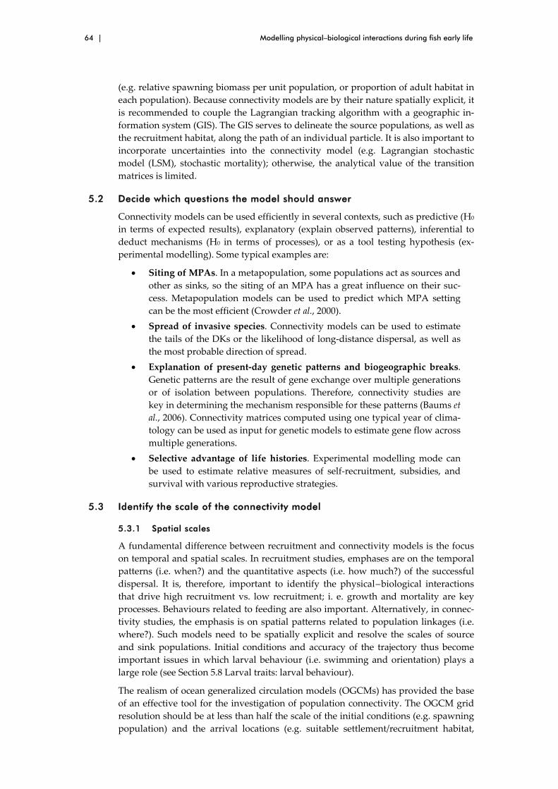
64 | Modelling physical–biological interactions during fish early life
(e.g. relative spawning biomass per unit population, or proportion of adult habitat in each population). Because connectivity models are by their nature spatially explicit, it is recommended to couple the Lagrangian tracking algorithm with a geographic in‐formation system (GIS). The GIS serves to delineate the source populations, as well as the recruitment habitat, along the path of an individual particle. It is also important to incorporate uncertainties into the connectivity model (e.g. Lagrangian stochastic model (LSM), stochastic mortality); otherwise, the analytical value of the transition matrices is limited.
5.2 Decide which questions the model should answer
Connectivity models can be used efficiently in several contexts, such as predictive (H0 in terms of expected results), explanatory (explain observed patterns), inferential to deduct mechanisms (H0 in terms of processes), or as a tool testing hypothesis (ex‐perimental modelling). Some typical examples are:
• Siting of MPAs. In a metapopulation, some populations act as sources and other as sinks, so the siting of an MPA has a great influence on their suc‐cess. Metapopulation models can be used to predict which MPA setting can be the most efficient (Crowder et al., 2000).
• Spread of invasive species. Connectivity models can be used to estimate the tails of the DKs or the likelihood of long‐distance dispersal, as well as the most probable direction of spread.
• Explanation of present‐day genetic patterns and biogeographic breaks. Genetic patterns are the result of gene exchange over multiple generations or of isolation between populations. Therefore, connectivity studies are key in determining the mechanism responsible for these patterns (Baums et al., 2006). Connectivity matrices computed using one typical year of clima‐tology can be used as input for genetic models to estimate gene flow across multiple generations.
• Selective advantage of life histories. Experimental modelling mode can be used to estimate relative measures of self‐recruitment, subsidies, and survival with various reproductive strategies.
5.3 Identify the scale of the connectivity model
5.3.1 Spatial scales
A fundamental difference between recruitment and connectivity models is the focus on temporal and spatial scales. In recruitment studies, emphases are on the temporal patterns (i.e. when?) and the quantitative aspects (i.e. how much?) of the successful dispersal. It is, therefore, important to identify the physical – biological interactions that drive high recruitment vs. low recruitment; i. e. growth and mortality are key processes. Behaviours related to feeding are also important. Alternatively, in connec‐tivity studies, the emphasis is on spatial patterns related to population linkages (i.e. where?). Such models need to be spatially explicit and resolve the scales of source and sink populations. Initial conditions and accuracy of the trajectory thus become important issues in which larval behaviour (i.e. swimming and orientation) plays a large role (see Section 5.8 Larval traits: larval behaviour).
The realism of ocean generalized circulation models (OGCMs) has provided the base of an effective tool for the investigation of population connectivity. The OGCM grid resolution should be at less than half the scale of the initial conditions (e.g. spawning population) and the arrival locations (e.g. suitable settlement/recruitment habitat,

ICES Cooperative Research Report No. 295 | 65
nursery grounds), which represent the starting and endpoints of the trajectories. Al‐ternatively, the population source size (grid or polygon size) should not be smaller than the resolution of the OGCM. This grid‐size requirement allows the particles to be released at each source population and recruited within a particular location at each time‐step without missing any unit population. In most cases, these locations are within the coastal realm in relatively shallow waters. OGCMs should cover larger areas than are significant for connectivity networks, but models that cover large areas usually do not adequately resolve the complexity of coastal dynamics, nor the resolu‐tion of the unit populations. Therefore, nested models are recommended, with higher resolution both on spawning and recruitment areas. Note that, at the scales of local retention, DKs could be limited by the spatial resolution of the model (e.g. smaller than the model’s mesh size).
5.3.2 Temporal scales
Ecological time‐scales are relevant to the demographic structure whereby a substan‐tial number of individuals are necessary to sustain (i.e. minimum of zero growth) a population. In this case, it is necessary to estimate the spatial probability of larval ex‐change or probability density functions (PDFs) over multiple years of daily forcing. Resulting transition matrices need to be scaled by species‐specific demographic pa‐rameters (e.g. birth, longevity, mortality). Geologic time‐scales are relevant to the evolutionary structure, whereby a few individuals exchanged per generation suffice to maintain genetic connectivity between populations. In this case, providing paths and relative percentage of larval exchange using one typical year of climatology with monthly forcing is appropriate.
Finally, connectivity models must explicitly span the relevant spatial and temporal scales of the target organisms (e.g. decadal variability of taxa with basin‐scale distri‐butions).
5.4 Gain knowledge of processes relevant to modelling connectivity
5.4.1 Initial conditions: spawning time and locations
Spawning locations should be mapped into GISs, serving both as initialization of the particle‐tracking system and as “source” locations in the connectivity model. A dis‐tance matrix Dij is built (where i = source location and j = arrival location) and is used to generate DKs (Figure 5.4.1). For more information on this topic, see Section 3.1 Ini‐tial conditions: spawning locations.
5.4.2 Suitable settlement locations
The endpoint or targets for the model need to be determined. For demersal species, this is usually the location and habitat where the pelagic early life‐history stage makes the transition to the demersal (bottom‐associated) stage. For pelagic species, this may be a nursery area, even if it is broad and diffuse (e.g. shallow coastal wa‐ters). The key point, however, is that particular habitat requirements for many species must be met at a particular stage in the life history. For some species, these require‐ments are well understood, but for many others, particularly in tropical areas, such requirements are not well known. The term “nursery area” has taken on a somewhat more precise definition recently (Beck et al., 2001; Dahlgren et al., 2006), and with ap‐plication of this definition, some reassessment of what were traditionally thought of as nurseries may be in order. Furthermore, settlement and nursery locations may not coincide for some species. Therefore, the modeller needs to consider carefully what

66 | Modelling physical–biological interactions during fish early life
the model is trying to achieve. For example, if the goal is to predict the distribution and numbers of a demersal species at settlement, the modeller has a different task than if the goal is to predict the numbers of individuals entering a fishery, or the numbers of individuals vulnerable to entrainment through the cooling system of an electricity‐generating station.
For connectivity models, the main goal is to map networks of larval linkages between populations, and although spawning and recruitment areas may be different, each paired set (spawning – recruitment locations) must represent a unit population. The modeller must obtain information on the settlement requirements of the species of interest, and then the spatial distribution of the appropriate habitat must be deter‐mined. This information may be available in the literature, but if not, appropriate surveys must be undertaken. An additional factor to consider is that, even if a par‐ticular location is understood to be suitable settlement habitat for species A, this can change with time by virtue of year‐to‐year fluctuations, anthropogenic influences (e.g. pollution or other habitat alteration), or by long‐term climate or other environ‐mental change (e.g. coral bleaching or cyclones can kill corals into which fish nor‐mally settle). It is therefore necessary to ensure that such occurrences have not altered the nature or distribution of the required habitat, because the initial studies of the habitat, if there are seasonal factors at play, incorporate a seasonal assessment of set‐tlement habitat quality or distribution. Suitable settlement locations should then be mapped into GIS layers that are fully integrated into the particle‐tracking modelling system, serving as “receiving” locations in the connectivity model.
Figure 5.4.1. Dispersal kernels or probability of dispersal to a suitable nursery habitat, showing the spatial scales associated with a 30‐day dispersal of fish larvae for various regions in the Car‐ibbean. The transition to the shaded area indicates the range of distances over which dispersal (and perhaps also survival) becomes irrelevant to demographic time‐scales. Mean dispersal dis‐tances are reflected in the modes that vary with locations, whereas self‐recruitment is the value at the origin.
5.4.3 Small-scale physics: turbulence
Physical processes occurring on scales smaller than the grid scale used in the model are often parameterized using a turbulent “diffusion” parameter, often called “eddy diffusivity”. This parameter should also include a factor to account for physical proc‐

ICES Cooperative Research Report No. 295 | 67
esses not included in the circulation model, and it does not represent the true advec‐tive processes that may be taking place.
5.4.4 Large-scale physics: grid size and domain
The physical processes discussed in this section refer only to large‐scale physical processes (i.e. larger than the grid resolution of the model).
Physical processes act on the transport/retention of larvae during their pelagic phase (e.g. wind‐driven circulation, tides, freshwater buoyancy, fronts), on settlement (e.g. bottom stress, sediment type), and on conditions affecting larvae survival (e.g. tem‐perature, short‐term event enhancing local increase of food). The combination of transport/retention, good conditions for settlement, and larvae survival can lead to sustainability or extinction of subpopulations, to exchanges between subpopulations, and to new subpopulations (colonization of new habitats).
The choice of which physical processes to explicitly resolve requires careful consid‐eration because it may not be necessary to include every process that might influence the transport path of larvae and the possibility of retention and settlement, taking into account the larval phase (pelagic) duration. According to the situation (e.g. coral reefs, shallow continental shelf, proximity of river mouth), not all of the physical processes, such as ocean currents, tides, wind, or freshwater inputs, will have the same importance. We recommend conducting sensitivity studies in order to deter‐mine the degree of importance of each physical process before choosing those that are key to the purpose of the study and the larval behaviour under consideration.
The physical processes to consider depend strongly on the region of interest (ROI) and also on the species under investigation. There is a strong link between physical processes, spawning frequency/duration, and larval behaviour (e.g. vertical migra‐tion). Spawning time/location, larval traits, and larval behaviour are the subject of other sections, and only some examples of situations where they should be taken into account are given in the list of physical processes below. This list, far from being ex‐haustive, is intended to help the modeller choose which physical processes to con‐sider as a function of the ROI. The “typical” spatio‐temporal scales of these physical processes are given in Section 1 Hydrodynamic models.
• Ocean currents. General circulation, coastal currents, meanders, jets, ed‐dies, shelf‐edge fronts.
• Tides. Tidal currents (can be important in shallow waters, reefs, etc., de‐pending on the topography), residual circulation, tidal fronts, vertical gra‐dients of horizontal currents, relationship with “larval behaviour” (synchronization of vertical migration of larvae with ebb – flood tidal cy‐cle), spawning timing (synchronization with spring neap tidal cycle), and spawning location (“choice” of spawning depth).
• Freshwater input. Presence of hydrological fronts in the proximity of river mouths, freshwater buoyancy circulation, water stratification density (may act as a barrier to vertical movements), periodic low‐salinity water intru‐sions (may affect depth of larvae), relationship with spawning timing (syn‐chronization with high/low river discharges).
• Wind. Wind‐driven circulation, internal waves, Langmuir cells, upwel‐lings/downwellings (and associated fronts and convergences).
• Fronts. Fronts (whatever their origin), which can act as a barrier that limits the larvae transport but are also the seat of circulations leading to conver‐

68 | Modelling physical–biological interactions during fish early life
gence/divergence zones; instabilities (e.g. eddies), can transport “isolated” water masses over long distances.
In addition to the “typical” distribution pattern resulting from averaged physical processes, the variability of these processes (e.g. extreme events, perturbations, insta‐bilities) can have a strong impact on larval transport or retention. Colonization of new habitats, for instance, could result from a particular event, and the spatial – temporal variability (e.g. interannual) of physical processes should be considered.
Model domain size and grid size must be chosen in accordance with the physical processes to be included. Processes smaller than the grid size must be parameterized, and processes acting at scales larger than the model domain should be considered according to appropriate boundary conditions (e.g. harmonic tides) or nesting. For the purpose of connectivity studies, grid size should be significantly smaller than the “assumed” distances between subpopulations and significantly smaller than a sub‐population. The model domain should at least encompass the whole region of possi‐ble exchanges between subpopulations and should include possible new habitats. For connectivity studies, it may be necessary to consider a whole region in order to en‐compass all existing subpopulations and possible new habitats, and also to consider a refined grid at the subpopulation level (e.g. shallow coastal waters, local retention, heterogeneity of sediment, needs of a fine vertical resolution). For this particular case, it could be interesting to consider model nesting.
Only thoroughly validated hydrodynamic models should be used for connectivity studies. The modeller should at least verify that current velocity (horizontal and ver‐tical) and/or trajectory path are correctly simulated. For more details, see Section 5.11 Model validation.
5.5 Lagrangian parameterization and online – offline methods
5.5.1 Parameterization of the Lagrangian statistics
In larval dispersal applications, the uncertainties in particle trajectories are usually parameterized, adding a stochastic component to the model‐predicted trajectories,
dx/dt = um + u’, (35)
where x is the particle position, um is the model velocity, and u’ is a stochastic veloc‐ity, which is typically described by a simple LSM (e.g. Griffa, 1996) and parameter‐ized by the horizontal grid‐scale diffusion according to Okubo (1971). However, the true eddy kinetic energy occurring at the subgrid scale can vary both spatially and temporally. Comparison between the kinetic energy content of the Eulerian velocity field for various grid sizes of the OGCM provides us with the energy cascade from the large‐scale to the submesoscale processes absent from the coarse‐grid simulation. Therefore, different regions with different processes (e.g. tide, shelf waves, eddies, currents, topography steering) are characterized by an energy‐spectrum structure from which can be extracted, in terms of percentage of total variance, the contribution of the submesoscale processes to the coarse‐grid flow. Spatial probability distribu‐tions of Eulerian decorrelation time‐scales and variances can be used to estimate the corresponding Lagrangian scales (Paris et al., 2007).
5.5.2 Online – offline methods
In connectivity modelling, thousands of particles are typically released simultane‐ously and repeatedly from hundreds of locations. Although computational speed has recently increased with the technique of parallel computing, offline modelling brings
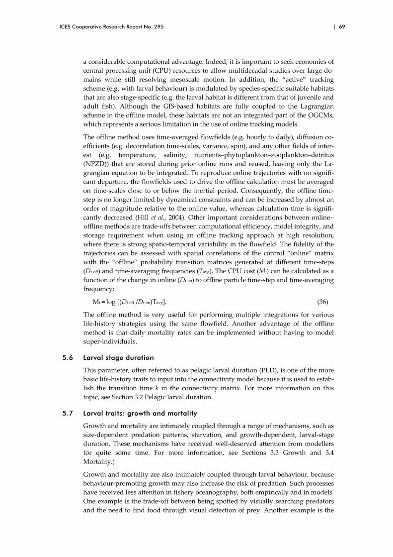
ICES Cooperative Research Report No. 295 | 69
a considerable computational advantage. Indeed, it is important to seek economies of central processing unit (CPU) resources to allow multidecadal studies over large do‐mains while still resolving mesoscale motion. In addition, the “active” tracking scheme (e.g. with larval behaviour) is modulated by species‐specific suitable habitats that are also stage‐specific (e.g. the larval habitat is different from that of juvenile and adult fish). Although the GIS‐based habitats are fully coupled to the Lagrangian scheme in the offline model, these habitats are not an integrated part of the OGCMs, which represents a serious limitation in the use of online tracking models.
The offline method uses time‐averaged flowfields (e.g. hourly to daily), diffusion co‐efficients (e.g. decorrelation time‐scales, variance, spin), and any other fields of inter‐est (e.g. temperature, salinity, nutrients–phytoplankton–zooplankton–detritus (NPZD)) that are stored during prior online runs and reused, leaving only the La‐grangian equation to be integrated. To reproduce online trajectories with no signifi‐cant departure, the flowfields used to drive the offline calculation must be averaged on time‐scales close to or below the inertial period. Consequently, the offline time‐step is no longer limited by dynamical constraints and can be increased by almost an order of magnitude relative to the online value, whereas calculation time is signifi‐cantly decreased (Hill et al., 2004). Other important considerations between online – offline methods are trade‐offs between computational efficiency, model integrity, and storage requirement when using an offline tracking approach at high resolution, where there is strong spatio‐temporal variability in the flowfield. The fidelity of the trajectories can be assessed with spatial correlations of the control “online” matrix with the “offline” probability transition matrices generated at different time‐steps (Dt‐off) and time‐averaging frequencies (Tavg). The CPU cost (Mt) can be calculated as a function of the change in online (Dt‐on) to offline particle time‐step and time‐averaging frequency:
Mt = log [(Dt‐off /Dt‐on)Tavg]. (36)
The offline method is very useful for performing multiple integrations for various life‐history strategies using the same flowfield. Another advantage of the offline method is that daily mortality rates can be implemented without having to model super‐individuals.
5.6 Larval stage duration
This parameter, often referred to as pelagic larval duration (PLD), is one of the more basic life‐history traits to input into the connectivity model because it is used to estab‐lish the transition time k in the connectivity matrix. For more information on this topic, see Section 3.2 Pelagic larval duration.
5.7 Larval traits: growth and mortality
Growth and mortality are intimately coupled through a range of mechanisms, such as size‐dependent predation patterns, starvation, and growth‐dependent, larval‐stage duration. These mechanisms have received well‐deserved attention from modellers for quite some time. For more information, see Sections 3.3 Growth and 3.4 Mortality.)
Growth and mortality are also intimately coupled through larval behaviour, because behaviour‐promoting growth may also increase the risk of predation. Such processes have received less attention in fishery oceanography, both empirically and in models. One example is the trade‐off between being spotted by visually searching predators and the need to find food through visual detection of prey. Another example is the

70 | Modelling physical–biological interactions during fish early life
risk of encountering tactile or ambush predators through increased swimming activ‐ity, which may be necessary to increase the encounter rate with potential prey items. There are also good reasons to argue that such behaviours are state‐ and size‐dependent, and that they interact with larval dispersal and drift trajectories. There is a need to adopt approaches from behavioural and evolutionary ecology to improve understanding of these processes.
Growth is often modelled in great detail, with much attention to processes and envi‐ronmental forcing. However, mortality is typically either not modelled at all or taken from statistical size‐dependent relationships with low mechanistic content and justi‐fication. However, the predation efficiency of invertebrates and fish typically varies predictably with a number of environmental factors, such as light, turbulence, and bottom depth, as well as larval behaviour (diel vertical migration, activity, and inter‐nal body condition). More efforts are required to include such processes in biophysi‐cal models.
5.8 Larval traits: larval behaviour
Fish larvae are not passive particles, and they have the potential to influence their dispersal (see review by Leis, 2006; Leis, 2007). Heterogeneous vertical positioning can result in divergent dispersal trajectories as well as differential survival (Paris and Cowen, 2004). Horizontal swimming can have a large influence on dispersal trajecto‐ries and on the success of settlement, particularly when larvae are able to orientate and in ecosystems, such as coral reefs, in which most fish larvae are very strong swimmers by the time they settle. Orientation can be further enhanced by schooling, because a school of larvae can act like a larger organism, with more precise sensory organs (Potter and Chitre, 2006). Schooling also influences feeding and predation rate, and hence has consequences for both growth and survival. Feeding behaviour and predator avoidance also contribute to differing survival rates. Finally, available suitable habitat and, at finer scales, habitat preferences during recruitment, can affect dispersal outcomes. Because larval behaviour influences both the endpoint of indi‐vidual trajectories and survival, it is particularly important to include behaviour in population connectivity models where these factors are vital. For more information, see Section 3.5 Behaviour and settlement.
5.9 Steps towards the state-of-the-art model
Exhaustive, perfect ground‐truth models are usually not produced on the first at‐tempt. We suggest here the order in which components should be implemented in a connectivity model, given its objectives. The minimum model should have relevant starting and ending locations and represent the main exchanges between them. Sub‐sequent steps should simulate active larval trajectories and, hence, produce more ac‐curate connectivity probabilities.
5.9.1 Step 1: minimum model
Start and end are defined by
• Locations and time of spawning (a priori breeding populations); • Location of potential settlement (e.g. GIS‐based habitat map, divided spa‐
tially into localities); • Integration time (e.g. PLD).
Trajectories should be computed using the Lagrangian approach, with a well‐parameterized, particle‐tracking model embedded in an OGCM (online), or operating
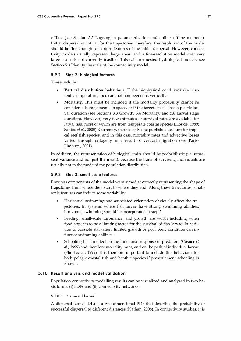
ICES Cooperative Research Report No. 295 | 71
offline (see Section 5.5 Lagrangian parameterization and online – offline methods). Initial dispersal is critical for the trajectories; therefore, the resolution of the model should be fine enough to capture features of the initial dispersal. However, connec‐tivity models usually represent large areas, and a fine‐resolution model over very large scales is not currently feasible. This calls for nested hydrological models; see Section 5.3 Identify the scale of the connectivity model.
5.9.2 Step 2: biological features
These include:
• Vertical distribution behaviour. If the biophysical conditions (i.e. cur‐rents, temperature, food) are not homogeneous vertically.
• Mortality. This must be included if the mortality probability cannot be considered homogeneous in space, or if the target species has a plastic lar‐val duration (see Sections 3.3 Growth, 3.4 Mortality, and 5.6 Larval stage duration). However, very few estimates of survival rates are available for larval fish, most of which are from temperate coastal species (Houde, 1989; Santos et al., 2005). Currently, there is only one published account for tropi‐cal reef fish species, and in this case, mortality rates and advective losses varied through ontogeny as a result of vertical migration (see Paris‐Limouzy, 2001).
In addition, the representation of biological traits should be probabilistic (i.e. repre‐sent variance and not just the mean), because the traits of surviving individuals are usually not in the mode of the population distribution.
5.9.3 Step 3: small-scale features
Previous components of the model were aimed at correctly representing the shape of trajectories from where they start to where they end. Along these trajectories, small‐scale features can induce some variability.
• Horizontal swimming and associated orientation obviously affect the tra‐jectories. In systems where fish larvae have strong swimming abilities, horizontal swimming should be incorporated at step 2.
• Feeding, small‐scale turbulence, and growth are worth including when food appears to be a limiting factor for the survival of fish larvae. In addi‐tion to possible starvation, limited growth or poor body condition can in‐fluence swimming abilities.
• Schooling has an effect on the functional response of predators (Cosner et al., 1999) and therefore mortality rates, and on the path of individual larvae (Flierl et al., 1999). It is therefore important to include this behaviour for both pelagic coastal fish and benthic species if presettlement schooling is known.
5.10 Result analysis and model validation
Population connectivity modelling results can be visualized and analysed in two ba‐sic forms: (i) PDFs and (ii) connectivity networks.
5.10.1 Dispersal kernel
A dispersal kernel (DK) is a two‐dimensional PDF that describes the probability of successful dispersal to different distances (Nathan, 2006). In connectivity studies, it is

72 | Modelling physical–biological interactions during fish early life
used to scale dispersal. The mode of the DK is relevant to ecological studies, whereas the tails (i.e. the frequency and spatial extent of long distance dispersal events) are relevant to biogeographical studies (e.g. multiple colonizations, disjunctions). Disper‐sal kernels can be represented for single locations or as “total” DKs, which incorpo‐rate the contribution of multiple dispersal vectors.
5.10.2 Transition probability matrix
A transition probability matrix (TPM) is a three‐dimensional PDF representing the probabilities of larvae moving from one state (e.g. gametes, early larvae) to another (e.g. recruitment‐stage larvae) in a dynamic system (Figure 5.10.1). The likelihood of larval exchange from one population to another, each associated with a given area, is represented in a TPM where columns are source locations (population i) and rows are destination locations (population j). The content of a given matrix element describes the probability of an individual larva making the transition from its source popula‐tion to the recruitment stage in the destination population. Elements along the diago‐nal of the matrix represent self‐recruitment within a local population. These matrices are usually sparse where zeros represent regions of no connectivity. The TPMs are of considerable value for metapopulation studies as well as for spatial management be‐cause they are three‐dimensional. TPMs also provide an ideal means of conducting sensitivity analyses using spatial autocorrelations.
Figure 5.10.1. Transition probability matrix. The contents of a given matrix element describe the probability of individual larvae making the transition from its source population (y‐axis) to the destination population (x‐axis), computed over several generations. Elements along the diagonal represent self‐recruitment within a population. The matrix is sparse where the grey area repre‐sents regions of no connectivity; the colour code indicates levels of connectivity from high (red) to low (blue). Higher connectivity on one side of the matrix corresponds to a drift in the direction of main currents.
Graph theory represents an effective means of visualizing population connectivity networks (e.g. Figure 5.10.2; see also Cowen et al., 2006). The relationships between populations are described by an adjacency matrix, derived from the probability tran‐sition matrix output by the connectivity model. The adjacency matrix (or edge) is a binary matrix in which each element is defined as Aij = 1, if populations i and j are connected by edges, or Aij = 0 if they are not connected. This matrix is mostly used to

ICES Cooperative Research Report No. 295 | 73
analyse connectivity networks (Urban and Keitt, 2001) and is extremely powerful for conservation issues such as strategic placement of MPAs and identification of source and sink populations, as well as key corridors (e.g. populations that are key to main‐tain the network).
Figure 5.10.2. Population Connectivity Network. Habitat patches are represented by nodes, for which size represents population density. When larvae from a given patch reach a downstream site, a dispersal connection is made. The thickness of the edge reflects the strength of the connec‐tion. This theoretical graph approach is useful to identify the spatial structure of the population sources, sinks, and corridors. The network is built directly for the transition probability matrix.
5.11 Model validation
There are two types of validation.
• Validation of trajectory path, using a combination of acoustic and hydro‐logical (e.g. acoustic Doppler current profiler (ADCP) and conductivity, temperature, depth (CTD)), Lagrangian (e.g. satellite tracked floats, fluo‐rescent wax particles), tagging or mass marking (e.g. otolith), and plankton (e.g. trawls, optical sampling) sampling tools. Trajectory validations are expensive and labour intensive. These direct methods of measuring con‐nectivity provide snapshots in time, but reveal mechanisms or physical – biological interactions that can be modelled.
• Validation of population connectivity results, using genetic tools that provide the genetic structure of populations (demographic time‐scales) or metapopulation (evolutionary time‐scales) depending on the gene used (review by Planes, 2002). Measurements of post‐larval supply at multiple sites can also produce a very consistent validation of the connectivity re‐sults (e.g. relative levels of recruitment into spatially explicit population units, Figure 5.11.1), without providing explicit knowledge of the source locations (i.e. TPM).

74 | Modelling physical–biological interactions during fish early life
Figure 5.11.1. Daily predicted larval supply of Sparisoma viride for the months February – December 2004 south of Sea Park in the Bahamas in ca. 50 km2 coral reef habitat. Note that the y‐axis represents simulated larvae and cannot be interpreted as an absolute measure of larval supply.
5.11.1 Trajectory path
Trajectory paths need to be validated (i) for their passive component and (ii) for their active component, which includes a series of larval behaviours. Validation should proceed as larval behaviours are introduced stepwise into the tracking scheme. See Section 5.8 Larval traits: larval behaviour.
Passive component of the trajectories:
• Ocean‐observing systems are always very useful. For example, time‐series of ADCPs moored in strategic locations can be used to improve the cou‐pled OGCM with data assimilation.
• To validate the small‐scale physical and biological processes operating at the starting (initial dispersal) or ending points (settlement processes) of the trajectories, gliders can be used, affording very high‐resolution, three‐dimensional hydrological data at specific spawning and recruitment sites.
• A series of floats deployed at various time frequencies and depths from distinct locations corresponding to an onshore – offshore gradient and dif‐ferent oceanographic regimes can be used to check the consistency of the trajectory predictions with the passive particle‐tracking code. Float data are also useful to compute diffusion parameterizations for the LSM.
Active component of the trajectories:
• Initial gamete dispersion can be assessed by conducting intensive Lagran‐gian field experiments with synoptic three‐dimensional hydrodynamic ob‐servations. The use of fluorescent wax particles calibrated with the egg density/size of the target species is recommended for the Lagrangian ex‐periment.
• To verify the accuracy of simulated trajectories of active larvae (e.g. onto‐genic vertical migration), repeated stratified samples of larval fish are nec‐essary. This sampling can be achieved using trawlnets, such as the Multi Opening and Closing Net and Environmental Sensing System (MOCNESS), or with well‐calibrated optical instruments, which take very high‐resolution shadow images.
• Proper validation of trajectory endpoints requires data on larval supply at multiple sites.

ICES Cooperative Research Report No. 295 | 75
• Other behaviours can be added stepwise to the model to perform sensitiv‐ity analyses, and the model outputs can then be compared with otolith mi‐crochemistry and genetic patterns or settled individuals.
5.11.2 Population connectivity results
Genetic validations can provide non‐directional (gene flow over several generations) and directional (DNA paternity analyses) connectivity networks, but do not reveal the mechanisms or physical – biological interactions that lead to connectivity. Genetic data based on fast‐evolving genes (such as microsatellite DNA) are extremely power‐ful in validating models of demographic connectivity. Paternity analyses or finger‐printing can provide detailed information on the parent – offspring relationships (Jones et al., 2005) and validate the direction and strength of connections. These inno‐vative genetic techniques are the best possible validations for connectivity models operating at the demographic scales. They provide a directional linkage between populations. To address questions at evolutionary time‐scales, mitochondrial DNA or slower‐evolving genes are useful to verify the spatial extent of the metapopulation (or species biogeography). However, caution is required for non‐directional types of validation. The TPM (or a powered TPM) assumes that migration is the main con‐tributing factor. Thus, the connectivity model assesses gene flow for neutral evolution (i.e. drift and recombination). Other processes, such as homoplasy and selection, even operating over relatively short time‐scales, can change genetic patterns. In addition, if genetic data do not resemble the connectivity model, it may not be the result of the connectivity model being flawed. Rather, it may be that demographic and post‐settlement processes (e.g. density, predation, latitudinal gradient, depth of settle‐ment) also contribute to the population structure.
5.12 Research needs
One of the limitations when modelling connectivity is the unavailability of nested OGCMs (highest resolution in the order of hundreds of metres resolving small‐scale processes at the spawning and recruitment areas) that operate at long time‐scales (re‐solving interannual variability over decadal time‐scales). Two‐way nested models are needed, with higher resolution both on spawning and recruitment areas. Information on species‐specific larval behaviour and mortality rates (including how both change with development) is also needed for more realistic biological connectivity models (Werner et al., 2007).
5.12.1 Initial dispersal
Lagrangian in situ measurements are needed to measure the dispersal statistics at spawning sites, which are not usually resolved by an OGCM. In particular, very little is known about diffusion in areas of steep slopes (e.g. promontories and capes), near the shelf break, and in shallow coral reef environments. To resolve initial dispersal, measurement of egg buoyancy is similarly important. Some fish species form tran‐sient spawning aggregations during a very narrow window in time, which usually coincides with a lunar phase and changes in water temperature and current intensity. For connectivity studies, there is a need to understand the cues utilized for spawning and to measure the associated physical features and dispersion parameters.
5.12.2 Settlement
More research is also needed (i) into the swimming and orientation of larval fish and their related cues (see Section 5.8 Larval traits: larval behaviour); and (ii) on the rates

76 | Modelling physical–biological interactions during fish early life
of larval mortality (see Section 3.4 Mortality) through ontogeny. Connectivity results are very sensitive to these parameters (Paris et al., unpublished data).

ICES Cooperative Research Report No. 295 | 77
6 Application 3: recruitment prediction
Sarah Hinckley, Bernard A. Megrey, and Thomas Miller
6.1 Definition
What do we mean by recruitment prediction? The first thing to consider in defining this term is the time horizon of the prediction. Short‐term predictions mean the use of individual‐based, coupled physical – biological models (ICPBMs) of fish early life his‐tory to predict annual recruitment, most usually to aid managers of fish stocks. These predictions may be made via indices or other measures of prerecruitment or recruit‐ment, derived from ICPBM output, that correlate well with other independent, rea‐sonable predictors of recruitment (derived from stock‐assessment models, reasonable independent juvenile or prerecruit surveys conducted with acoustic or trawl, or other net‐based survey methods). These may be used alone or in conjunction with other predictors, such as spawning‐stock biomass. Actual numerical estimates (of the cor‐rect magnitude) derived from ICPBMs may be possible, but only if certain conditions are met (e.g. the super‐individual method, proportionality indices, or other methods of relating model indices to real population numbers are used, and spawning‐biomass or egg‐production estimates as initial conditions are included). A benefit of these indices is that they could serve as a replacement for expensive juvenile surveys.
Under this definition, the forecast window for recruitment predictions would be lim‐ited to the number of years from spawning to recruitment for each species of interest. This is because of the fundamental lack of predictability of regional and small‐scale ocean physics. These prediction windows will be different for each species owing to differences in the unique aspects of a species’ life history.
Longer‐term recruitment predictions that are likely under different future scenarios (e.g. of climate, fishing, or ocean variability) may also be derived from ICPBMs through the use of the models to gain a mechanistic understanding of the important biophysical processes underlying recruitment variability. This knowledge may, for example, help us to understand simple correlations between biophysical factors and recruitment, and when such correlations may or may not hold up.
The development of recruitment predictors from ICPBMs requires careful considera‐tion of what we mean by recruitment. There are many ways of defining recruitment. The operational definition depends on the purpose or goal of the prediction. Are we predicting recruitment for management purposes? If so, then recruitment is often defined as the number of fish entering the exploited segment of the population, where the meaning of “exploited segment” depends on the distinctive attributes of each fishery (i.e. gear type, time and space scales). If examining life‐history character‐istics or gaining ecological understanding is the goal, recruitment could be defined as the number of fish reaching a juvenile nursery area, the number reaching maturity, or the number reaching a particular age, size, or stage.
6.2 Objectives of recruitment prediction
There can be several different objectives for recruitment prediction, and these will affect not only how we select a predictive index from the model, but how the ICPBM itself is constructed and its relevant physical and biological details. Recruitment pre‐diction may be undertaken to test our understanding of the processes that affect re‐cruitment. ICPBMs may be developed to clarify mechanistic processes underlying correlations between physical or biological factors and recruitment. Recruitment pre‐

78 | Modelling physical–biological interactions during fish early life
diction may be applied or pragmatic, for example, to aid in the reduction of the num‐ber of recruitment scenarios that must be performed in the stock‐assessment model‐ling process.
Who are the clients/consumers of the forecasts? To maximize the usefulness of re‐cruitment forecasts, they need to be tailored to the user. The needs of scientific re‐searchers, resource managers, and commercial fishery concerns may be different. For example, a forecast prepared for a scientist might be used as a null hypothesis to demonstrate whether or not the forecast embodies a sufficient understanding of the processes and mechanisms that cause good and bad year classes. In contrast, deci‐sion‐makers in commercial fisheries may require a forecast only as a basis for future buying decisions regarding capital expenditures for equipment or ship improve‐ments. In this case, the emphasis is not so much on perfect understanding. For exam‐ple, if a forecast tells them to expect several years of good recruitment, they may decide to purchase automatic fish‐filleting equipment optimized for smaller fish. If recruitment is expected to be poor, they may conclude that they will be exploiting older individuals from the population and should purchase filleting machines opti‐mized for larger fish. In both cases, their goal is to maximize product recovery, and having the right equipment for the circumstances plays a large role in attaining their goal.
6.3 Indices of recruitment from ICPBMs
When using ICPBMs to aid in the prediction of recruitment, an index that appears to correlate well with recruitment can be used. Often, these indices relate to some un‐derlying theory about recruitment success. Some examples of recruitment or prere‐cruitment indices that have been, or could be, derived from ICPBMs are (i) the number of larvae or juveniles that reach a specified nursery area, weighted by their residence time there (Parada et al., in review); (ii) the number that reach a nursery area by a particular date, size, or age (Bartsch et al., 2004; Baumann et al., 2006); (iii) indices of larval drift or retention, such as the number going in a predefined direction (Wespestad et al., 2000; Wilderbuer et al., 2002; Stockhausen, pers. comm.) that ex‐perience different levels of bottom depth anomalies (Baumann et al., 2006), or a sur‐vival rate after a certain number of days of drift (Allain et al., 2007); (iv) indices of overlap of larvae with their prey (Hinrichsen et al., 2005); or (v) indices of juvenile particle density at the end of a simulation to look for density‐dependent processes related to recruitment (Baumann et al., 2006).
Indices may be compared with data, for example, surveys of prerecruits or recruits. Indices may also be compared with stock‐assessment model estimates of recruitment. In this case, caution is needed. The same data may be used in the ICPBM and the stock‐assessment model (e.g. spawning‐stock biomass); therefore, the indices pro‐duced by the two models may not be independent.
The proper choice of recruitment indices will depend on the objectives of the work, the life history of the species, and theories (conceptual models) of what processes are critical to recruitment variability. The development of a conceptual model (see Sec‐tion 6.4) can aid in the choice of indices.
6.4 The need for a conceptual model
Development of a conceptual model of the processes controlling recruitment for each species and area is key to the use of ICPBMs in recruitment prediction, and also to the choice of the proper indices derived from the models. Development of a conceptual

ICES Cooperative Research Report No. 295 | 79
model is a way of organizing what is important, the importance of the roles played by particular processes, and what life stages are affected. If this is neglected, impor‐tant factors or processes may be missed in the ICBPM.
• Life stages and their duration • Variation in mortality at each stage • Biological and physical factors affecting each stage and the “intensity” of
the effect • Processes important within each stage
If different processes at different life stages are thought to be important, it may be necessary to develop different conceptual models for the same species in different areas. For example, the walleye pollock conceptual models for the Gulf of Alaska (http://www.pmel.noaa.gov/foci/forecast/mgt.html; Figure 6.4.1) and Bering Sea (http://www.pmel.noaa.gov/foci/sebscc/results/megrey/bs_concept.html; Figure 6.4.2) contain the same life stages and duration, but they differ with respect to which life stages experience the most variability in mortality and the factors that influence mor‐tality and survival. Therefore, somewhat different ICPBMs have been developed, and different indices may be necessary to predict recruitment.
Figure 6.4.1. Gulf of Alaska walleye pollock conceptual model (from Megrey and Wespestad, 1997).

80 | Modelling physical–biological interactions during fish early life
Figure 6.4.2. Southeast Bering Sea walleye pollock conceptual model (from Megrey et al., 1996).
Conceptual models are not stagnant. They evolve as new information and under‐standing become available. For example, the original Gulf of Alaska pollock concep‐tual model (Figure 6.4.1) has recently been modified to include the effects of regime‐scale climate impacts, as well as predation and competition effects (species‐to‐species interactions) known to be important at the ecosystem level (Bailey, 2000; Bailey et al., 2005; Megrey and Macklin, unpublished report).
6.5 Forecasting accuracy
How accurate do recruitment forecasts have to be before they become useful? This is a difficult yet relevant question that needs immediate research attention. A recent paper by De Oliveira and Butterworth (2005) offers a concrete example of a possible approach. The premise in this paper was that environmental indices that provide short‐term predictions of recruitment have the potential to improve the average yield from highly productive resources that sustain recruit fisheries without an associated increase in risk (of resource “collapse”). This paper’s authors asked the question, how accurate does an environment‐dependent, spawner – recruit relationship have to be before it affects management decisions? Specifically, what are the benefits of using environmental indices to set appropriate total allowable catches? Through a con‐trolled simulation experiment, they concluded that an environmental index needs to explain roughly 50 % or more of the total variation in recruitment (r 2 ≥ 0.5) before the management procedure starts revealing benefits in terms of the summary perform‐ance statistics for risk and average catch. Having similar quantitative information on recruitment forecasts from ICPBM models would help frame the circumstances in which it could prove to be of benefit.
If an index derived from an ICPBM is to be used for recruitment forecasting, it is critical to assess its accuracy and to build trust in its ability to forecast.
6.6 Techniques for forecasting
Forecasts can take many different forms. They can take the form of quantitative an‐nual estimates of absolute abundance (e.g. there will be 5.5 billion recruits next year). We do not believe these are very useful, and they are difficult to produce with any

ICES Cooperative Research Report No. 295 | 81
accuracy and precision. They can also be qualitative. For example, the forecast could be given in terms of recruitment being in a particular state — below average, average, and above average (low, medium, and high) — with appropriate methods used to de‐fine, in operational terms, states such as long‐term averages or quantiles (33 %, 50 %, or 66 %) based on observed recruitment trends. Rothschild and Mullen (1985) give a good example of how recruitment information (from data or models) can be usefully described by non‐parametric classification based on Markov chains. Finally, a re‐cruitment forecast could be the result of an ensemble estimate from numerous sto‐chastic‐forecast implementations. The forecast can be delivered as a probability statement; for example, the probability of achieving a given recruitment level or state based on x conditions and y assumptions is 10 %. The most appropriate form depends on many factors including many that have been discussed above, such as for whom the forecast is being prepared, how it will be used, the required accuracy, and the required forecast horizon.
A caution should be offered regarding the use of recruitment estimates from stock‐assessment models to calculate metrics as described above. Changes/updates in an‐nual stock‐assessment/cohort‐analysis models and resulting recruitment estimates make the most recent estimates of “recruitment” somewhat of a moving target. Stock‐assessment models estimate recruitment by summing all fish from a cohort (all indi‐viduals with the same birth year) that have died as a result of the fishery (i.e. the catches) and then including the fish that have died from natural causes (also esti‐mated by assuming a particular rate of natural mortality). In other words, the re‐cruitment estimate is the population that would have existed in order to generate the observed catches. The data point of most interest is usually the current year. If a co‐hort is still contributing to the catch, then in next year’s assessment, an additional year of catches and losses from natural mortality will increase the recruitment esti‐mate relative to the current year. The recruitment estimate will gradually increase over time and finally stabilize once the cohort is completely fished out (i.e. no more individuals of the cohort survive to add to the catches).
6.7 Philosophy of modelling
Approaches to understanding mechanisms that regulate recruitment in fish have in‐creasingly taken an individual‐based approach. This approach can be justified on two general grounds. First, field research into recruitment processes in fish has demon‐strated that the individuals that survive early life often possess a unique suite of genotypic or phenotype traits that are not simply a random draw from the distribu‐tion present at spawning. For example, numerous studies involving otolith micro‐structure have demonstrated that survivors are selected from a narrow window of the original distribution of birthdates. Other research has revealed selection based on growth rate, size at settlement, spawning location, and maternal influence. Together, these studies have highlighted the fact that we would probably not understand mechanisms regulating recruitment by measuring mean rates; instead, we needed to characterize the sources, patterns, and consequences of variation among individuals in early life traits and understand why the unique subset of traits possessed by re‐cruits conferred a survival advantage.
The second justification for individual‐based approaches invokes the importance of spatial processes in regulating recruitment. Sinclair and Iles (1988) proposed a mem‐ber‐vagrant hypothesis in which population persistence relied upon the existence of closed trajectories that allowed surviving larvae to complete their life cycle. Those larvae that “followed” appropriate trajectories became members of the reproductive

82 | Modelling physical–biological interactions during fish early life
population; individuals that “followed” inappropriate trajectories were lost to the reproductive population. This hypothesis, built on the existing understanding of the importance of population structure within a species, emphasizes the importance of the spatial location of larvae at different points in development on their subsequent survival.
Coupled physical – biological models addressing questions involving fish early life histories have typically adopted an individual‐based approach. The majority of such models have used a grid‐based hydrodynamic model to predict currents at nodes on the grid, which are then used in a Lagrangian particle‐tracking algorithm to move particles that represent the early life stages around the model domain. For example, in one of the earliest applications of such models, Bartsch and colleagues (Bartsch, 1988, 1993; Bartsch et al., 1989) considered the trajectories of herring larvae in the North Sea. The model results indicated the importance of a retentive area off the east coast of Scotland. Subsequently, ICPBMs have become more sophisticated in both the representation of the current fields and the biological representation of individual fish. Such models have been used to quantify the contribution of different spawning locations to recruitment, the role of physical processes in regulating feeding, and the influence of mortality on spatial distributions.
However, it is vital to assess and separate the biological motivations for individual‐based approaches to the study of fish populations from the computational motiva‐tion. Computationally, individual‐based approaches are attractive because they ele‐gantly combine the grid‐based, spatially specific predictions of hydrodynamic models with biological processes. In so doing, such models portray individuals that differ with respect to their trajectories and thus their exposures to environmental forcing. To ease computational demands, population‐level predictions are derived by expanding the predictions for a single particle by a multiplier to represent the contri‐bution to the population. This approach implicitly assumes that all variability in early life history is spatially determined. Simply stated, this approach assumes that all variability is caused by differences among the trajectories followed by individuals, and not by inherent biological interindividual variability. The approach emphasizes the importance of member – vagrant‐type ideas at the expense of phenotypic variabil‐ity among individuals. Not all models make this assumption. A few do include and sample from distributions of traits. For example, in their detailed model of feeding, Fiksen and Mackenzie (2002) sampled from distributions of reactive distances to es‐timate feeding incidence. However, ICPBMs of the entire early life history that incor‐porate inherent interindividual variability have yet to be developed. Whether or not the development of such models is important depends entirely on how total pheno‐typic variability is partitioned between spatially derived sources and inherent inter‐individual differences. This partitioning is, as yet, unexplored and unquantified.

ICES Cooperative Research Report No. 295 | 83
7 Looking to the future: recommendations and research needs
Elizabeth W. North, Alejandro Gallego, and Pierre Petitgas
The goal of this section is to summarize the major recommendations and research needs that were identified during the WKAMF workshop and in the process of de‐veloping this Manual of Recommended Practices. We address and elaborate on the six major themes necessary to advance the field of modelling physical – biological in‐teractions in the early life stages of fish that were identified by WKAMF participants.
1 ) Validation and sensitivity methods 2 ) Model complexity 3 ) Physics 4 ) Energetics 5 ) Mortality 6 ) Behaviour and cues
High‐quality data and improved and widely implemented methods for model valida‐tion are fundamental needs that limit the ultimate utility of fish early‐life models and the advancement of the field. Consistency of model with observations is important, and data quality is paramount. Methods of model – data comparison need to be ap‐plied and developed. In addition, the validity of quantitative metrics should be ad‐dressed. Central to the issue of validation is the availability of good‐quality data at the appropriate resolution. All too often, modelling is seen as a cheap(er) alternative to empirical work, particularly in the marine field, where data acquisition is challeng‐ing and expensive. Modellers are expected to work with data that are sometimes old or of questionable quality, and with coarse spatial and/or temporal resolution.
These problems affect not only model validation, but also initialization (boundary and initial conditions) and operation (forcing data). It is vital to communicate to the non‐modelling community that the quality of the biophysical modelling output de‐pends strongly on a basic knowledge of physical and biological processes, and on the quality of empirical data used for model initialization and validation. Fortunately, technical advances in field‐, laboratory‐, and data‐processing tools are likely to result in considerable progress in the near future, although they may not completely replace the more traditional, labour‐intensive and knowledge‐rich methodologies. Another challenge is the development of data‐assimilation methodology to incorporate obser‐vations of physical and biological parameters (especially those from automated data‐acquisition systems) into biophysical models (see Section 4 Application 1: adaptive sampling). This is a critical requirement if we are to make biophysical models opera‐tional.
The model is a platform that coherently integrates multidisciplinary knowledge. Ap‐propriate model complexity is a research need. Models should be as simple as possi‐ble but as complex as necessary. Additional layers of complexity should only be added after (i) assessment of need, based on the objectives of the modelling endeav‐our; and (ii) analysis of the sensitivity of the model to the process(es) under consid‐eration. The GLOBEC “rhomboid approach” (with complexity greatest at the level of the target organism and decreasing towards higher and lower trophic levels; De Young et al., 2004) was suggested as a conceptual framework for addressing model complexity. Although model complexity may be constrained by lack of knowledge of physical and/or biological processes and/or operational limitations (e.g. computing

84 | Modelling physical–biological interactions during fish early life
hardware or software), these limitations should be seen as a challenge to overcome, not as reasons for making do with the status quo. The modelling process should ex‐plicitly document knowledge gaps, thus providing the direction for advancing the field.
After choosing the appropriate complexity, the next step is to document model sensi‐tivity. Sensitivity analysis of model outputs to variations in model complexity or pa‐rameter values should be considered thoroughly. Methods for sensitivity analysis of complex models have been developed in industry, including group screening, simu‐lation designs, partial regressions, and benchmarking. Their applicability and useful‐ness for biophysical IBMs is a challenging research need. An introduction on the topic can be found in Kleijnen (2005).
Hydrodynamic model predictions critically influence biological predictions. Basic improvements in understanding of turbulence and in predicting mixing and circula‐tion patterns will advance the field of larval fish modelling. Ensemble methods (com‐bining a suite of simulations that have slightly different starting conditions or model assumptions; Gneiting and Raftery, 2005) and probabilistic approaches (e.g. Brickman et al., 2007) offer promising techniques that should be implemented when possible. We need to (i) develop measurements of turbulence and any other relevant physical and biological parameters at scales that are appropriate to predator –prey interac‐tions; and (ii) parameterize encounter, capture, and feeding processes at scales from 1 mm to 1 m (see below). It is important, therefore, to develop sampling devices or approaches that allow increased resolution in space or time, in addition to data proc‐essing and visualization tools, that allow researchers to interpret large volumes of complex multidimensional and multidisciplinary data.
The choices of Lagrangian model type and implementation techniques are not consis‐tent, despite the fact that these models provide the basic structure for individual‐based, coupled physical – biological models (ICPBMs). For Lagrangian particle track‐ing, a standard set of test cases should be established and published (see Section 2 Particle tracking), both in the literature and on a dedicated website, for advection and subgrid‐scale turbulence models in the horizontal and vertical directions. The tests should be easy to implement, cover the practical issues, and become standard proce‐dure. From a technical standpoint, theory development/elucidation is needed to de‐termine whether or not numerical methods satisfy theoretical requirements (e.g. when subgrid‐scale turbulence and directed swimming are combined in particle‐tracking models). The need for a systematic assessment of Lagrangian model types and implementation techniques is elucidated by the differences in recommendations between sections of this manual. The authors of Section 2 recommend using a ran‐dom displacement model (RDM), whereas those of Section 5 recommend the use of a Lagrangian stochastic model (LSM). These apparent contradictions may stem from dissimilarity in the time‐ and space‐scale of the hydrodynamic models used by the authors. The choice of appropriate model remains an active area of research; clarifica‐tion is needed if the field is to evolve.
Fundamental information is needed on the biological processes of mortality, behav‐iour, and energetics to advance models of the early life of fish. These stage‐dependent, and often species‐specific, processes pose challenges for investigation, but recent advances in field and laboratory techniques will most probably revolutionize the field of larval fish modelling. The need for improved understanding of basic processes is exemplified by the discrepancy in the assumption that fish larvae are food‐limited (Section 3.5 Behaviour and settlement) or are not food‐limited (Section

ICES Cooperative Research Report No. 295 | 85
3.3 Growth). This and other differences in perception between sections could simply be based on the ecosystem in which the authors are most experienced (e.g. temperate vs. tropical) and point to the need to assess and unify our understanding of biological processes across taxa and ecosystems. Despite these differences, it is becoming broadly recognized that it may not be sufficient just to incorporate “means” into our models. Instead, the effect of individual variability (including “extreme” values) needs to be assessed, because the survivors may not just be the “lucky few”, but may be drawn from the extremes of a given distribution (e.g. fastest growers). In many current biophysical models, individual variability is purely the result of spatial (envi‐ronmental history) variability.
The following are some specific recommendations relevant to biological processes.
• Better information on the underlying mechanisms that drive spatial and temporal patterns in spawning, including adult characteristics (e.g. behav‐iour, maternal effects), is critical for defining appropriate initial conditions for biophysical modelling of early life stages of fish (e.g. the formulation and validation of egg‐production models).
• We need to understand the mechanisms of internal (physiology) and ex‐ternal (environmental signals, prey, predators) drivers. The influence of the light environment, as affected by geography, seasonality, primary pro‐duction, suspended sediment, and associated sources of freshwater, needs to be evaluated.
• There is a clear need for field/laboratory studies of behaviour, especially related to horizontal orientation/directed swimming and the physi‐cal/biological factors that cue larval behaviour. We should challenge estab‐lished parameter values (e.g. swimming speeds) in experimental and more realistic settings, and compare them (at least for some species). In addition, some generally accepted assumptions should be assessed, such as the ab‐sence of directed swimming among temperate fish species or the parame‐terization of behaviour based on similarity in phylogeny (when data are lacking for the species of interest).
• Techniques for validation of larval transport predictions and connectivity patterns are needed. Although methods for validating hydrodynamic and particle‐tracking models are either well established (for hydrodynamics) or in development (for particle tracking), a systematic set of methods is needed for validation of biological trajectories (i.e. ones that include behav‐iour). High‐frequency sampling permitted by underway identification sys‐tems or genetic‐based approaches may provide the means of accomplishing this.
• A variety of growth models have proven to be very sensitive to assimila‐tion efficiency as well as to changes in size spectrum of prey; a better un‐derstanding of the causal mechanisms is required. Mechanistic (bioenergetic) modelling of growth is attracting considerable interest, probably as a result of the proliferation of ecosystem models that provide prey fields for the larvae. The sensitivity of these models to assumptions and uncertainties in parameter values/functional relationships should be carefully assessed.
• Predictions of predator feeding rates (i.e. mortality on larvae) from labora‐tory, field, and simple models differ significantly (by tenfold in some cases). Consequently, modelling predator feeding requires improved ob‐

86 | Modelling physical–biological interactions during fish early life
servations and greater effort to validate any model developments. Mortal‐ity is often not incorporated in biophysical models of fish early life stages or is modelled as a size‐dependent function with low (or no) mechanistic content. The development of mechanistic models of predation is fraught with difficulties: predation efficiency of invertebrates and fish is typically influenced by a suite of environmental factors (light, turbulence, the prey environment, prey “behaviour” in general), and the dynamic representa‐tion of predator fields is a momentous task. However, it is clear that, for an adequate representation of mortality in the models, more effort is required to include such processes.
• The role of density‐dependence in nature needs to be further investigated and, where appropriate, incorporated into models. This is also related to the requirement to increase our understanding of the ecology of the early juvenile stage. The arrival at (and survival within) suitable nursery areas has been identified as critical to year‐class strength in numerous species, but our knowledge of the main ecological processes during that period is still largely inadequate.
The use of ICPBMs has increased our understanding of the interacting factors that influence fish early life. Although research needs are many, the field holds great promise for advancing our understanding of fish‐population variability and the in‐fluence of changing climate on fish stocks and the humans who depend on them. Fur‐ther advances in the field of larval fish modelling and prediction will probably arise from dynamic teams of scientists who can unite laboratory, field, and modelling ex‐pertise. Importantly, for the utility and impact of these models, the translation of re‐sults to managers, stakeholders, and the general public is desirable. Scientists should collaborate in the communication process to ensure correct interpretation and use of model results.
Acknowledgements
We thank Emory Anderson, Katharine Smith, and William Anthony and the ICES Publications department for assistance with editing, and the US National Science Foundation (NSF) for providing support for the production of this manual (OISE‐0527221). Support for Elizabeth North was provided by the University of Maryland Center for Environmental Science (UMCES). Support for Alejandro Gallego was pro‐vided by the Fisheries Research Services (FRS), an agency of the Scottish Government Marine Directorate.
This Manual is a product of the “Workshop on advancements in modelling physical –biological interactions in fish early life history: recommended practices and future directions” (WKAMF), which was held under the auspices of the International Coun‐cil for the Exploration of the Sea (ICES) Working Group on Physical – Biological Inter‐actions and the ICES Working Group on Recruitment Processes. It was hosted by the French Research Institute for Exploitation of the Sea (IFREMER), with support from the IFREMER, US NSF, US National Marine Fisheries Service, FRS (UK), and UMCES. It was endorsed by GLOBEC and Eur‐Oceans.

ICES Cooperative Research Report No. 295 | 87
8 References
Ådlandsvik, B. 2000. VertEgg – a toolbox for simulation of vertical distributions of fish eggs, version 1.0. Available online at http://www.imr.no/ bjorn/VertEgg/vertegg.pdf.
Aksnes, D. L., and Giske, J. 1993. A theoretical model of aquatic visual feeding. Ecological Modelling, 67: 233 – 250.
Alexandre, D., and Ghysen, A. 1999. Somatotopy of the lateral line projection in larval zebraf‐ish. Proceedings of the National Academy of Sciences of the USA, 96(13): 7558 – 7562.
Allain, G., Petitgas, P., Lazure, P., and Grellier, P. 2007. Biophysical modelling of larval drift, growth, and survival for the prediction of anchovy recruitment in the Bay of Biscay (NE Atlantic). Fisheries Oceanography, 16: 489 – 505.
Almany, G. R. 2003. Priority effects in coral reef fish communities. Ecology, 94: 1920 – 1935.
Anderson, J. T. 1988. A review of size dependent survival during pre‐recruit stages of fishes in relation to recruitment. Journal of Northwest Atlantic Fishery Science, 8: 55 – 66.
Arakawa, A. 1966. Computational design for long‐term numerical integration of the equations of fluid motion: two‐dimensional incompressible flow. Part I. Journal of Computational Physics, 135: 103 – 114.
Armsworth, P. R., James, M. K., and Bode, L. 2001. When to press on or turn back: dispersal strategies for reef fish larvae. The American Naturalist, 157: 434 – 450.
Arvedlund, M., McCormick, M. I., Fautin, D. G., and Bildsoe, M. 1999. Host recognition and possible imprinting in the anemonefish Amphiprion melanopus. Marine Ecology Progress Series, 188: 207 – 218.
Atema, J., Kingsford, M. J., and Gerlach, G. 2002. Larval reef fish could use odour for detection, retention, and orientation to reefs. Marine Ecology Progress Series, 241: 151 – 160.
Bailey, K. M. 2000. Shifting control of recruitment of walleye pollock Theragra chalcogramma after a major climatic and ecosystem change. Marine Ecology Progress Series, 198: 215 – 224.
Bailey, K. M., and Houde, E. D. 1989. Predation on eggs and larvae of marine fishes and the recruitment problem. Advances in Marine Biology, 25: 1 – 83.
Bailey, K. M., Ciannelli, L., Bond, N., Belgrano, A., and Stenseth, N. C. 2005. Recruitment of walleye pollock in a physically and biologically complex ecosystem: a new perspective. Progress in Oceanography, 67: 24 – 42.
Bartsch, J. 1988. Numerical simulation of the advection of vertically migrating herring larvae in the North Sea. Meeresforschung, 32: 30 – 45.
Bartsch, J. 1993. Application of a circulation and transport model system to the dispersal of herring larvae in the North Sea. Continental Shelf Research, 13: 1335 – 1361.
Bartsch, J. 2002. Modelling the temperature mediation of growth in larval fish. Fisheries Oceanography, 11: 310 – 314.
Bartsch, J. 2005. The influence of spatio‐temporal egg production variability on the modelled survival of the early life history stages of mackerel (Scomber scombrus) in the eastern North Atlantic. ICES Journal of Marine Science, 62: 1049 – 1060.
Bartsch, J., and Coombs, S. 2004. An individual‐based model of the early life history of mack‐erel (Scomber scombrus) in the eastern North Atlantic, simulating transport, growth, and mortality. Fisheries Oceanography, 13: 365 – 379.
Bartsch, J., Brander, K., Heath, M., Munk, P., Richardson, K., and Svendsen, E. 1989. Modeling the advection of herring larvae in the North Sea. Nature, 340: 632 – 636.

88 | Modelling physical–biological interactions during fish early life
Bartsch, J., Reid, D., and Coombs, S. 2004. Simulation of mackerel (Scomber scombrus) recruit‐ment with an individual‐based model and comparison with field data. Fisheries Oceanog‐raphy, 13: 380 – 391.
Batchelder, H. P. 2006. Forward‐in‐time‐/backward‐in‐time‐trajectory (FITT/BITT) modeling of particles and organisms in the coastal ocean. Journal of Atmospheric and Oceanic Tech‐nology, 23: 727 – 741.
Baumann, H., Hinrichsen, H‐H., Möllmann, C., Köster, F. W., Malzahn, A. M., and Temming, A. 2006. Recruitment variability in Baltic Sea sprat (Sprattus sprattus) is tightly coupled to temperature and transport patterns affecting the larval and early juvenile stages. Canadian Journal of Fisheries and Aquatic Sciences, 63: 2191 – 2201.
Baums, I., Paris, C. B., and Cherubin, L. M. 2006. A bio‐oceanographic filter to larval dispersal in a reef‐building coral. Limnology and Oceanography, 51: 1969 – 1981.
Beaugrand, G., Brander, K. M., Lindley, J. A., Souissi, S., and Reid, P. C. 2003. Plankton effect on cod recruitment in the North Sea. Nature, 426: 661 – 664.
Beck, M. W., Heck, K. L., Able, K. W., Childers, D. L., Eggleston, D. B., Gillanders, B. M., Halpern, B., et al. 2001. Towards better identification, conservation and management of es‐tuarine and marine nurseries. BioScience, 51: 633 – 641.
Bellwood, D. R., and Fisher, R. 2001. Relative swimming speeds in fish larvae. Marine Ecology Progress Series, 211: 299 – 303.
Bennett, A. 2006. Lagrangian Fluid Dynamics. Cambridge Monographs on Mechanics. Cam‐bridge University Press, Cambridge, UK. 286 pp.
Berloff, P., and McWilliams, J. 2002. Material transport in oceanic gyres. Part II: Hierarchy of stochastic models. Journal of Physical Oceanography, 32: 797 – 830.
Beyer, J. E. 1989. Recruitment stability and survival − simple size‐specific theory with examples from the early life dynamics of marine fish. Dana, 7: 45 – 147.
Blumberg, A. F., and Mellor, G. L. 1987. A description of a three‐dimensional coastal ocean circulation model. In Three‐Dimensional Coastal Ocean Models, Volume 4, pp. 1 – 16. Ed. by N. Heaps. American Geophysical Union, Washington, DC. 208 pp.
Boehlert, G. W., Watson, W., and Sun, L. C. 1992. Horizontal and vertical distributions of larval fishes around an isolated oceanic island in the Tropical Pacific. Deep Sea Research I, 39: 436 – 466.
Botello, G., and Krug, P. J. 2006. “Desperate larvae” revisited: age, energy and experience affect sensitivity to settlement cure in larvae of the gastropod Alderia sp. Marine Ecology Pro‐gress Series, 312: 149 – 159.
Bowen, A. J., Griffin, D. A., Hazen, D. G., Matheson, S. A., and Thompson, K. R. 1995. Ship‐board nowcasting of shelf circulation. Continental Shelf Research, 15: 115 – 128.
Boyra, G., Rueda, L., Coombs, S., Sundby, S., Ådlandsvik, B., and Uriarte, A. 2003. Modelling the vertical distribution of eggs of anchovy (Engraulis encrasicolus) and sardine (Sardina pil‐chardus). Fisheries Oceanography, 12: 381 – 395.
Bradbury, I. R., Snelgrove, R. V. R., and Pepin, P. 2003. Passive and active behavioural contri‐butions to patchiness and spatial pattern during the early life history of marine fishes. Ma‐rine Ecology Progress Series, 257: 233 – 245.
Breitburg, D. 1989. Demersal schooling prior to settlement by larvae of the naked goby. Envi‐ronmental Biology of Fishes, 26: 97 – 103.
Brickman, D., and Frank, K. T. 2000. Modelling the dispersal and mortality of Browns Bank egg and larval haddock (Melanogrammus aeglefinus). Canadian Journal of Fisheries and Aquatic Sciences, 57: 2519 – 2535.

ICES Cooperative Research Report No. 295 | 89
Brickman, D., and Smith, P. 2002. Lagrangian stochastic modeling in coastal oceanography. Journal of Atmospheric and Oceanic Technology, 19: 83 – 99.
Brickman, D., Shackell, N. L., and Frank, K. T. 2001. Modelling the retention and survival of Browns Bank haddock larvae using an early life stage model. Fisheries Oceanography, 10: 284 – 296.
Brickman, D., Marteinsdottir, G., and Taylor, L. 2007. Formulation and application of an effi‐cient optimized biophysical model. Marine Ecology Progress Series, 347: 275 – 284.
Browman, H. I., and Skiftesvik, A. B. 1996. The effects of turbulence on the predation cycle of fish larvae: comments on some of the issues. Marine Ecology Progress Series, 139: 309 – 312.
Browman, H. I., St‐Pierre, J‐F., Skiftesvik, A. B., and Racca, R. G. 2003. Behaviour of Atlantic cod (Gadus morhua) larvae: an attempt to link maternal condition with larval quality. In The Big Fish Bang. Proceedings of the 26th Annual Larval Fish Conference, pp. 71 – 95. Ed. by H. I. Browman and A. B. Skiftesvik. Institute of Marine Research, Bergen, Norway. 476 pp.
Browman, H. I., Yen, J., St‐Pierre, J‐F., and Kuhn, P. In prep. Predatory behaviour of the car‐nivorous copepod Euchaeta norvegica, and escape responses of their prey (larval Atlantic cod, Gadus morhua). Marine Ecology Progress Series.
Chen, C., Beardsley, R. C., and Cowles, G. 2006. An unstructured‐grid, finite‐volume coastal ocean model (FVCOM) system. Advances in Computational Oceanography, 19: 78 – 89.
Campana, S. E., and Hurley, P. C. F. 1989. An age‐ and temperature‐mediated growth model for cod (Gadus morhua) and haddock (Melanogrammus aeglefinus) larvae in the Gulf of Maine. Canadian Journal of Fisheries and Aquatic Sciences, 46: 603 – 613.
Christensen, A., Daewel, U., Jensen, H., Mosegaard, H., St John, M., and Schrum, C. 2007. Hy‐drodynamic backtracking of fish larvae by individual‐based modelling. Marine Ecology Progress Series, 347: 221 – 232.
Codling, E. A., Hill, N. A., Pitchford, J. W., and Simpson, S. D. 2004. Random walk models for the movement and recruitment of reef fish larvae. Marine Ecology Progress Series, 279: 215 – 224.
Conway, D. V. P., Coombs, S. H., Lindley, J. A., and Llewellyn, C. A. 1999. Diet of mackerel (Scomber scombrus) larvae at the shelf edge to the southwest of the British Isles and the in‐cidence of piscivory and coprophagy. Vie Milieu, 49: 213 – 220.
Cosner, C., DeAngelis, D. L., Ault, J. S., and Olson, D. B. 1999. Effects of spatial grouping on the functional response of predators. Theoretical Population Biology, 56: 65 – 75.
Cowan, J. H., Rose, K. A., Rutherford, E. S., and Houde, E. D. 1993. Individual‐based model of young‐of‐the‐year striped bass population dynamics. II. Factors affecting recruitment in the Potomac River, Maryland. Transactions of the American Fisheries Society, 122: 439 – 458.
Cowan, J. H., Houde, E. D., and Rose, K. A. 1996. Size‐dependent vulnerability of marine fish larvae to predation: an individual‐based numerical experiment. ICES Journal of Marine Science, 53: 23 – 37.
Cowen, R. K., Paris, C. B., Fortuna, J. L., and Olson, D. B. 2003. The role of long distance disper‐sal in replenishing marine populations. Gulf and Caribbean Research, 14: 129 – 137.
Cowen, R. K., Paris, C. B., and Srinivasan, A. 2006. Scaling of connectivity in marine popula‐tions. Science, 311: 522 – 527.
Crowder, L. B., Lyman, S. J., Figueira, W. F., and Priddy, J. 2000. Source‐sink population dy‐namics and the problem of siting marine reserves. Bulletin of Marine Science, 66: 799 – 820.
Cummings, J. A. 2005. Operational multivariate ocean data assimilation. Quarterly Journal of the Royal Meteorological Society, 131: 2583 – 3604.

90 | Modelling physical–biological interactions during fish early life
Dahlgren, C. P., Kellison, G. T., Adams, A. J., Gillanders, B. M., Kendall, M. S., Layman, C. A., Ley, J. A., et al. 2006. Marine nurseries and effective juvenile habitats: concepts and appli‐cations. Marine Ecology Progress Series, 312: 291 – 295.
DeAngelis, D. L., and Rose, K. A. 1992. Which individual‐based approach is most appropriate for a given problem? In Individual‐Based Models and Approaches in Ecology: Popula‐tions, Communities and Ecosystems, pp. 66 – 87. Ed. by D. L. DeAngelis and L. J. Gross. Chapman and Hall, New York, USA. 525 pp.
Delhez, E. J. M., Damm, P., de Goede, E., de Kok, J. M., Dumas, F., Gerritsen, H., Jones, J. E., et al. 2004. Variability of shelf‐seas hydrodynamic models: lessons from the NOMADS2 Pro‐ject. Journal of Marine Systems, 45: 39 – 53.
De Oliveira, J. A. A., and Butterworth, D. S. 2005. Limits to the use of environmental indices to reduce risk and/or increase yield in the South African anchovy fishery. African Journal of Marine Science, 27: 191 – 203.
DeYoung, B., Heath, M., Werner, F., Chai, F., Megrey, B., and Monfray, P. 2004. Challenges of modelling decadal variability in ocean basin ecosystems. Science, 304: 1463 – 1466.
Doherty, P. J. 1983. Diel, lunar and seasonal rhythms in the reproduction of two tropical damselfishes: Pomacentrus flavicauda and P. wardi. Marine Biology, 75: 215 – 224.
Doherty, P. J., and McIlwain, J. 1996. Monitoring larval fluxes through the surf zones of Austra‐lian coral reefs. Marine and Freshwater Research, 47: 383 – 390.
Doherty, P. J., Dufour, V., Galzin, R., Hixon, M. A., Meekan, M. G., and Planes, S. 2004. High mortality during settlement is a population bottleneck for a tropical surgeonfish. Ecology, 85: 2422 – 2428.
Dower, J. F., Miller, T. J., and Leggett, W. C. 1997. The role of microscale turbulence in the feed‐ing ecology of larval fish. Advances in Marine Biology, 31: 169 – 220.
Edwards, A., and Brindley, J. 1996. Oscillatory behaviour in a three‐component plankton popu‐lation model. Dynamics and Stability of Systems, 11: 347 – 370.
Edwards, A., and Yool, A. 2000. The role of higher predation in plankton population models. Journal of Plankton Research, 22: 1085 – 1112.
Edwards, C., Powell, T., and Batchelder, H. 2000. The stability of an NPZ model subject to real‐istic levels of vertical mixing. Journal of Marine Research, 58: 37 – 60.
Ellien, C., Thibaut, E., Dumas, F., Salomon, J‐C., and Nival, P. 2004. A modelling study of the respective role of hydrodynamic processes and larval mortality on larval dispersal and re‐cruitment on benthic invertebrates: example of Pectinaria koreni (Annelida: Polycheta) in the Bay of Seine (English Channel). Journal of Plankton Research, 26: 117 – 132.
Elliott, J. K., Elliott, J. M., and Mariscal, R. N. 1995. Host selection, location, and association behaviours of anemonefishes in field selection experiments. Marine Biology, 122: 377 – 389.
Fiksen, Ø., and Folkvord, A. 1999. Modelling growth and ingestion processes in herring Clupea harengus larvae. Marine Ecology Progress Series, 184: 273 – 289.
Fiksen, Ø., and MacKenzie, B. R. 2002. Process‐based models of feeding and prey selection in larval fish. Marine Ecology Progress Series, 243: 151 – 164.
Fiksen, Ø., Utne, A. C. W., Aksnes, D. L., Eiane, K., Helvik, J. V., and Sundby, S. 1998. Model‐ling the influence of light, turbulence and ontogeny on ingestion rates in larval cod and herring. Fisheries Oceanography, 7: 355 – 363.
Fiksen, Ø., Jørgensen, C., Kristiansen, T., Vikebø, F., and Huse, G. 2007. Linking behavioural ecology and oceanography: larval behaviour determines growth, mortality and dispersal. Marine Ecology Progress Series, 347: 195 – 205.
Fisher, R., and Bellwood, D. R. 2002. The influence of swimming speed on sustained swimming performance of late‐stage reef fish larvae. Marine Biology, 140: 801 – 807.

ICES Cooperative Research Report No. 295 | 91
Fisher, R., and Bellwood, D. R. 2003. Undisturbed swimming behaviour and nocturnal activity of coral reef fish larvae. Marine Ecology Progress Series, 263: 177 – 188.
Fisher, R., and Hogan, D. 2007. Morphological predictors of swimming speed: a case study of pre‐settlement juvenile coral reef fishes. Journal of Experimental Marine Biology and Ecol‐ogy, 210: 2436 – 2443.
Fisher, R., and Wilson, S. K. 2004. Maximum sustainable swimming speeds of late‐stage larvae of nine species of reef fishes. Journal of Experimental Marine Biology and Ecology, 312: 171 – 186.
Fisher, R., Bellwood, D. R., and Job, S. D. 2000. Development of swimming abilities in reef fish larvae. Marine Ecology Progress Series, 202: 163 – 173.
Flesch, T. K., Wilson, J. D., and Yee, E. 1995. Backward‐time Lagrangian stochastic dispersion models and their application to estimate gaseous emissions. Journal of Applied Meteorol‐ogy, 34: 1320 – 1332.
Flierl, G., Grunbaum, D., Levin, S., and Olson, D. 1999. From individuals to aggregations: the interplay between behaviour and physics. Journal of Theoretical Biology, 196: 397 – 454.
Folkvord, A. 2005. Comparison of size‐at‐age of larval Atlantic cod (Gadus morhua) from differ‐ent populations based on size‐ and temperature‐dependent growth models. Canadian Journal of Fisheries and Aquatic Sciences, 62: 1037 – 1052.
Fuiman, L. A., and Cowan, J. H. 2003. Behaviour and recruitment success in fish larvae: repeat‐ability and covariation of survival skills. Ecology, 84: 56 – 73.
Fuiman, L. A., and Higgs, D. M. 1997. Ontogeny, growth and the recruitment process. In Early Life History and Recruitment in Fish Populations, pp. 225 – 249. Ed by R. C. Chamber and E. A. Trippel. Chapman and Hall, London, UK.
Fuiman, L. A., and Magurran, A. E. 1994. Development of predator defences in fishes. Reviews in Fish Biology and Fisheries, 4: 145 – 185.
Galbraith, P., Browman, H. I., Racca, R. G., Skiftesvik, A. B., and St‐Pierre, J‐F. 2004. The effect of turbulence on the energetics of foraging in Atlantic cod (Gadus morhua) larvae. Marine Ecology Progress Series, 281: 241 – 257.
Gallager, S. M., Yamazaki, H., and Davis, C. S. 2004. Contribution of fine‐scale vertical struc‐ture and swimming behaviour to formation of plankton layers on Georges Bank. Marine Ecology Progress Series, 267: 27 – 43.
Gallego, A., and Heath, M. R. 1994. The development of schooling behavior in Atlantic Herring Clupea harengus. Journal of Fish Biology, 45(4): 569 – 588.
Gallego, A., Heath, M. R., Wright, P., and Marteinsdóttir, G. 1999. An empirical model of growth in the pelagic early life history stages of North Sea haddock. ICES Document CM 1999/Y:13. 9 pp.
Gibson, G., Musgrave, D., and Hinckley, S. 2005. Non‐linear dynamics of a pelagic ecosystem model with multiple predator and prey types. Journal of Plankton Research, 27: 427 – 447.
Gneiting, T., and Raftery, A. E. 2005. Weather forecasting with ensemble methods. Science, 310: 248 – 249.
Gray, C. A. 1996. Do thermoclines explain the vertical distributions of larval fishes in the dy‐namic coastal waters of south‐eastern Australia? Australian Journal of Marine and Fresh‐water Research, 47: 183 – 190.
Gray, C. A., and Kingsford, M. J. 2003. Variability in thermocline depth and strength, and the relationships with vertical distributions of fish larvae and mesozooplankton in dynamic coastal waters. Marine Ecology Progress Series, 247: 221 – 224.
Griffa, A. 1996. Stochastic modeling in physical oceanography: applications of stochastic parti‐cle models to oceanographic problems. In Stochastic Modelling in Physical Oceanography,

92 | Modelling physical–biological interactions during fish early life
pp. 114 – 140. Ed. by R. J. Adler, P. Müller, and B. Rozovoskii. Birkha ̈user, Boston, MA, USA. 468 pp.
Grimm, V., and Railsback, S. F. 2005. Individual‐Based Modeling and Ecology. Princeton Uni‐versity Press, Princeton, NJ, USA. 428 pp.
Hadfield, M. G. 1998. The D. P. Wilson Lecture. Research on settlement and metamorphosis of marine invertebrate larvae past, present and future. Biofouling, 12: 9 – 29.
Hanski, I. 1989. Metapopulation dynamics: Does it help to have more of the same? Trends in Ecology and Evolution, 4: 113 – 114.
Hawryshyn, C. W. 2000. Ultraviolet polarization vision in fishes: possible mechanisms for cod‐ing e‐vector. Philosophical Transactions of the Royal Society of London, Series B, Biologi‐cal Sciences, 355: 1187 – 1190.
Heath, M. R., and Gallego, A. 1997. From the biology of the individual to the dynamics of the population: bridging the gap in fish early life studies. Journal of Fish Biology, 51: 1 – 29.
Heath, M. R., and Gallego, A. 1998. Biophysical modelling of the early life stages of haddock, Melanogrammus aeglefinus, in the North Sea. Fisheries Oceanography, 7: 110 – 125.
Helbig, J. A., and Pepin, P. 1998a. Partitioning the influence of physical processes on the esti‐mation of ichthyoplankton mortality rates. I. Theory. Canadian Journal of Fisheries and Aquatic Sciences, 55: 2189 – 2205.
Helbig, J. A., and Pepin, P. 1998b. Partitioning the influence of physical processes on the esti‐mation of ichthyoplankton mortality rates. II. Application to simulated and field data. Ca‐nadian Journal of Fisheries and Aquatic Sciences, 55: 2206 – 2220.
Hermann, A. J., Hinckley, S., Megrey, B. A., and Stabeno, P. J. 1996. Interannual variability of the early life history of walleye pollock near Shelikof Strait as inferred from a spatially ex‐plicit, individual‐based model. Fisheries Oceanography, 5: 39 – 57.
Hermann, A., Hinckley, S., Megrey, B., and Napp, J. 2001. Applied and theoretical considera‐tions for constructing spatially explicit individual‐based models of marine larval fish that include multiple trophic levels. ICES Journal of Marine Science, 58: 1030 – 1041.
Hill, A. E. 1994. Horizontal zooplankton dispersal by diel vertical migration in S2 tidal currents on the northwest European continental shelf. Continental Shelf Research, 14: 491 – 506.
Hill, H., Hill, C., Follows, M., and Dutkiewicz, S. 2004. Is there a computational advantage to offline tracer modeling at very high resolution? Geophysical Research Abstracts, 6, EGU04‐A‐06348, 2004. 1017.
Hillgruber, N., and Kloppmann, M. 2001. Small‐scale patterns in distribution and feeding of Atlantic mackerel (Scomber scombrus L.) larvae in the Celtic sea with special regard to inter‐cohort cannibalism. Helgoland Marine Research, 55: 135 – 149.
Hillgruber, N., Kloppmann, M., Wahl, E., and von Westernhagen, H. 1997. Feeding of larval blue whiting and Atlantic mackerel: a comparison of foraging strategies. Journal of Fish Biology, 51(Suppl. A): 230 – 249.
Hinckley, S., Hermann, A. J., and Megrey, B. A. 1996. Development of a spatially explicit, indi‐vidual‐based model of marine fish early life history. Marine Ecology Progress Series, 139: 47 – 68.
Hinckley, S., Hermann, A. J., Mier, K. L., and Megrey, B. A. 2001. Importance of spawning loca‐tion and timing to successful transport to nursery areas: a simulation study of Gulf of Alaska walleye pollock. ICES Journal of Marine Science, 58: 1042 – 1052.
Hinckley, S., Napp, J., Hermann, A., and Parada, C. In press. Simulation of physically mediated variability in prey resources for a larval drift fish: a three‐dimensional NPZ model. Fisher‐ies Oceanography.
ICES Cooperative Research Report No. 295 | 93
Hindell, J. S., Jenkins, G. P., Moran, S. M., and Keough, M. J. 2003. Swimming ability and be‐haviour of post‐larvae of a temperate marine fish re‐entrained in the pelagic environment. Oecologia, 135: 158 – 166.
Hinrichsen, H‐H., Schmidt, J. O., Petereit, C., and Möllmann, C. 2005. Survival probability of Baltic larval cod in relation to spatial overlap patterns with their prey obtained from drift model studies. ICES Journal of Marine Science, 62: 878 – 885.
Hofmann, E. E., and Friedrichs, M. A. M. 2002. Predictive modeling for marine ecosystems. In The Sea, Volume 12: Biological‐Physical Interactions in the Ocean, pp. 537 – 565. Ed. by A. R. Robinson, J. J. McCarthy, and B. J. Rothschild. Harvard University Press, Cambridge, MA, USA. 662 pp.
Holbrook, S. J., and Schmitt, R. J. 1999. In situ nocturnal observations of reef fishes using infra‐red video. In Proceedings of the 5th Indo‐Pacific Fish Conference, Noumea, pp. 805 – 812. Ed. by B. Seret and J‐Y. Sire. Societie Francaise Ichtyologie, Paris, France. 866 pp.
Houde, E. D. 1989. Comparative growth, mortality, and energetics of marine fish larvae: tem‐perature and implied latitudinal effects. Fishery Bulletin US, 87: 471 – 495.
Houde, E. D. 1994. Difference between marine and freshwater fish larvae: implications for re‐cruitment. ICES Journal of Marine Science, 51: 91 – 97.
Houde, E. D. 1997. Patterns and trends in larval‐stage growth and mortality of teleost fish. Journal of Fish Biology, 51(Suppl. A): 52 – 83.
Houde, E. D. 2002. Mortality. In Fishery Science: The Unique Contributions of Early Life Stages, pp. 64 – 87. Ed. by L. A. Fuiman and R. G. Werner. Blackwell Publishing, Oxford, UK. 326 pp.
Houde, E. D., and Secor, D. H. 1996. Episodic water quality events and striped bass recruit‐ment: larval mark‐recapture experiments in the Nanticoke River. Final Report to Maryland Department of Natural Resources, Contract Number CB93 – 006 – 002. University of Mary‐land System, Center for Environmental and Estuarine Studies, Chesapeake Biological Laboratory, Solomons, MD, USA. (UMCEES) CBL 96 – 083.
Houde, E. D., and Zastrow, C. E. 1993. Ecosystem‐ and taxon‐specific dynamic and energetics properties of larval fish assemblages. Bulletin of Marine Science, 53: 290 – 335.
Humston, R., Olson, D., and Ault, J. 2004. Behavioural assumptions in models of fish move‐ment and their influence on population dynamics. Transactions of the American Fisheries Society, 133: 1304 – 1328.
Hunter, J., Craig, P., and Phillips, H. 1993. On the use of random‐walk models with spatially variable diffusivity. Journal of Computational Physics, 106: 366 – 376.
Huth, A., and Wissel, C. 1992. The simulation of the movement of fish schools. Journal of Theo‐retical Biology, 156: 365 – 385.
Irisson, J‐O., Levan, A., De Lara, M., and Planes, S. 2004. Strategies and trajectories of coral reef fish larvae optimizing self‐recruitment. Journal of Theoretical Biology, 227: 205 – 218.
Job, S. D., and Bellwood, D. R. 2000. Light sensitivity in larval fishes: implications for vertical zonation in the pelagic zone. Limnology and Oceanography, 45: 362 – 371.
Jones, G. P., Planes, S., and Thorrold, S. R. 2005. Coral reef fish larvae settle close to home. Cur‐rent Biology, 15: 1314 – 1318.
Jones, J. E. 2002. Coastal and shelf‐sea modelling in the European context. Oceanography and Marine Biology: An Annual Review, 40: 37 – 141.
Jørgensen, C., Dunlop, E. S., Opdal, A. F., and Fiksen, Ø. 2008. The evolution of spawning mi‐grations: the role of individual state, population structure, and fishing‐induced changes. Ecology, 89(12): 3436 – 3448.

94 | Modelling physical–biological interactions during fish early life
Kendall, A. W., Ahlstrom, E. H., and Moder, H. G. 1984. Introduction: the early life history stages of fishes and their characters. In Ontogeny and Systematics of Fishes, pp. 11 – 22. Ed. by H. G. Moder, J. W. Richards, D. M. Cohen, M. P. Fahay, A. W. Kendall, and S. L. Richardson. Allen Press, Lawrence, KS. 760 pp.
Kingsford, M. J., Leis, J. M., Shanks, A., Lindeman, K., Morgan, S., and Pineda, J. 2002. Sensory environments, larval abilities and local self‐recruitment. Bulletin of Marine Science, 70: 309 – 340.
Kitchell, J. F., Stewart, D. J., and Weininger, D. 1977. Applications of a bioenergetics model to yellow perch (Perca flavescens) and walleye (Stizostedion vitreum vitreum). Journal of the Fisheries Research Board of Canada, 34: 1922 – 1935.
Kleijnen, J. 2005. An overview of the design and analysis of simulation experiments for sensi‐tivity analysis. European Journal of Operational Research, 164: 287 – 300.
Klimley, A., Anderson, S., Pyle, P., and Henderson, R. 1992. Spatio‐temporal patterns of white shark (Carcharodon carcharias) predation at the south Farallon islands, California, USA. Copeia, 1992: 680 – 690.
Kloeden, P., and Platen, E. 1995. Numerical Solution of Stochastic Differential Equations. Springer, New York, USA. 632 pp.
Kristiansen, T., Fiksen, Ø., and Folkvord, A. 2007. Modelling feeding, growth and habitat selec‐tion in larval cod: observations and model predictions in a macrocosm environment. Ca‐nadian Journal of Fisheries and Aquatic Sciences, 64: 136 – 151.
Lara, M. R. 2001. Morphology of the eye and visual acuities in the settlement‐intervals of some coral reef fishes (Labridae, Scaridae). Environmental Biology of Fishes, 62: 365 – 378.
Lefebvre, A., Ellien, C., Davoult, D., Thiébaut, E., and Salomon, J‐C. 2003. Pelagic dispersal of the brittle‐star Ophiothrix fragilis larvae in a megatidal area (English Channel, France) ex‐amined using an advection/diffusion model. Estuarine, Coastal, and Shelf Science, 57: 421 – 433.
Legg, B. J., and Raupach, M. R. 1982. Markov‐chain simulation of particle dispersion in inho‐mogeneous flows: the mean drift velocity induced by a gradient in Eulerian velocity vari‐ance. Boundary Layer Meteorology, 66: 3 – 13.
Leis, J. M. 1986. Epibenthic schooling by larvae of the clupeid fish Spratelloides gracilis. Japanese Journal of Ichthyology, 33: 67 – 69.
Leis, J. M. 2004. Vertical distribution behaviour and its spatial variation in late‐stage larvae of coral‐reef fishes during the day. Marine and Freshwater Behaviour and Physiology, 37: 65 – 88.
Leis, J. M. 2006. Are larvae of demersal fishes plankton or nekton? Advances in Marine Biol‐ogy, 51: 57 – 141.
Leis, J. M. 2007. Behaviour as input for modelling dispersal of fish larvae: behaviour, biogeog‐raphy, hydrodynamics, ontogeny, physiology and phylogeny meet hydrography. Marine Ecology Progress Series, 347: 185 – 193.
Leis, J. M., and Carson‐Ewart, B. M. 1998. Complex behaviour by coral‐reef fish larvae in open‐water and near‐reef pelagic environments. Environmental Biology of Fishes, 53: 259 – 266.
Leis, J. M., and Carson‐Ewart, B. M. 1999. In situ swimming and settlement behaviour of larvae of an Indo‐Pacific coral‐reef fish, the coral trout (Pisces, Serranidae, Plectropomus leopardus). Marine Biology, 134: 51 – 64.
Leis, J. M., and Carson‐Ewart, B. M. 2000. Behaviour of pelagic larvae of four coral‐reef fish species in the ocean and an atoll lagoon. Coral Reefs, 19: 247 – 257.
Leis, J. M., and Carson‐Ewart, B. M. 2002. In situ settlement behaviour of damselfish larvae (Pisces: Pomacentridae). Journal of Fish Biology, 61: 325 – 346.

ICES Cooperative Research Report No. 295 | 95
Leis, J. M., and Carson‐Ewart, B. M. 2003. Orientation of pelagic larvae of coral‐reef fishes in the ocean. Marine Ecology Progress Series, 252: 239 – 253.
Leis, J. M., and Lockett, M. M. 2005. Localization of reef sounds by settlement‐stage larvae of coral‐reef fishes (Pomacentridae). Bulletin of Marine Science, 76: 715 – 724.
Leis, J. M., and McCormick, M. I. 2002. The biology, behaviour and ecology of the pelagic, lar‐val stage of coral‐reef fishes. In Coral Reef Fishes: New Insights into Their Ecology, pp. 171 – 199. Ed. by P. F. Sale. Academic Press, San Diego, CA, USA. 549 pp.
Leis, J. M., Sweatman, H. P. A., and Reader, S. E. 1996. What the pelagic stages of coral reef fishes are doing out in blue water: daytime field observations of larval behavioural capa‐bilities. Australian Journal of Marine and Freshwater Research, 47: 401 – 411.
Leising, A., and Franks, P. 1999. Larval Atlantic cod (Gadus morhua) and haddock (Melanogrammus aeglefinus) growth on Georges Bank: a model with temperature, prey size, and turbulent forcing. Canadian Journal of Fisheries and Aquatic Sciences, 56: 25 – 36.
Letcher, B. H., Rice, J. A., Crowder, L. B., and Rose, K. A. 1996. Variability in survival of larval fish: disentangling components with a generalized individual‐based model. Canadian Journal of Fisheries and Aquatic Sciences, 53: 787 – 801.
Levins, R. 1969. Some demographic and genetic consequences of environmental heterogeneity for biological control. Bulletin of the Entomology Society of America, 71: 237 – 240.
Lewis, D. M. 2003. Planktonic encounter rates in homogeneous isotropic turbulence: the case of predators with limited fields of sensory perception. Journal of Theoretical Biology, 222: 73 – 97.
Li, M., Zhong, L., and Boicourt, W. C. 2005. Simulations of Chesapeake Bay estuary: sensitivity to turbulence mixing parameterizations and comparison with observations. Journal of Geophysical Research, 110: C12004.
Lima, S. L., and Dill, L. M. 1990. Behavioral decisions made under the risk of predation − a re‐view and prospectus. Canadian Journal of Zoology, 68: 619 – 640.
Lough, R. G., Buckley, L. J., Werner, F. E., Quinlan, J. A., and Edwards, K. P. 2005. A general biophysical model of larval cod (Gadus morhua) growth applied to populations on Georges Bank. Fisheries Oceanography, 14: 241 – 262.
Lynch, D. R., Ip, J. T. C., Naimie, C. E., and Werner, F. E. 1996. Comprehensive coastal circula‐tion model with application to the Gulf of Maine. Continental Shelf Research, 16: 875 – 906.
MacKenzie, B. R., and Kiørboe, T. 2000. Larval fish feeding and turbulence: a case for the downside. Limnology and Oceanography, 45: 1 – 10.
MacKenzie, B. R., Miller, T. J., Cyr, S., and Leggett, W. C. 1994. Evidence for a dome‐shaped relationship between turbulence and larval fish ingestion rates. Limnology and Oceanog‐raphy, 39: 1790 – 1799.
Maes, J., Limburg, K. E., Van de Putte, A., and Ollevier, F. 2005. A spatially explicit, individual‐based model to assess the role of estuarine nurseries in the early life history of North Sea herring, Clupea harengus. Fisheries Oceanography, 14: 17 – 31.
Masuda, R., Shoji, J., Nakayama, S., and Tanaka, M. 2003. Development of schooling behavior in Spanish mackerel Scomberomorus niphonius during early ontogeny. Fisheries Science, 69: 772 − 776.
McBride, R. S., and Able, K. W. 1998. Ecology and fate of butterflyfishes, Chaetodon spp., in the temperate, western North Atlantic. Bulletin of Marine Science, 63: 401 – 416.
McCormick, M. I., and Mackey, L. J. 1997. Post‐settlement transition in coral reef fishes: over‐looked complexity in niche shifts. Marine Ecology Progress Series, 153: 247 – 257.
McGurk, M. D. 1986. Natural mortality of marine pelagic fish eggs and larvae: role of spatial patchiness. Marine Ecology Progress Series, 34: 227 – 242.

96 | Modelling physical–biological interactions during fish early life
Meekan, M., and Fortier, L. 1996. Selection for fast growth during the larval life of Atlantic cod Gadus morhua on the Scotian Shelf. Marine Ecology Progress Series, 137: 25 – 37.
Megrey, B. A., and Hinckley, S. 2001. Effect of turbulence on feeding of larval fishes: a sensitiv‐ity analysis using an individual‐based model. ICES Journal of Marine Science, 58: 1015 – 1029.
Megrey, B. A., and Macklin, S. A. 2007. Critical analysis of FOCI recruitment predictions for the Gulf of Alaska, 1992 – 2007. Unpublished report. B. Megrey, AFSC, Seattle, WA, USA.
Megrey, B. A., and Wespestad, V. G. 1997. Conceptual model of relationships between pollock recruitment and biophysical correlates in the Southeast Bering Sea. SEBSCC (Southeast Bering Sea Carrying Capacity) Annual Reports, Fiscal Year 1997.
Megrey, B. A., Hollowed, A. B., Hare, S. R., Macklin, S. A., and Stabeno, P. J. 1996. Contribu‐tions of FOCI research to forecasts of year‐class strength of walleye pollock in Shelikof Strait, Alaska. Fisheries Oceanography, 5(Suppl. 1): 189 – 203.
Miller, T. J., Crowder, L. B., Rice, J. A., and Marschall, E. A. 1988. Larval size and recruitment mechanisms in fishes: towards a conceptual framework. Canadian Journal of Fisheries and Aquatic Sciences, 45: 1657 – 1670.
Montgomery, J. C., Jeffs, A., Simpson, S. D., Meekan, M. G., and Tindle, C. 2006. Sound as an orientation cue for the pelagic larvae of reef fishes and decapod crustaceans. Advances in Marine Biology, 51: 143 – 239.
Morse, W. W. 1989. Catchability, growth and mortality of larval fishes. Fishery Bulletin US, 87: 417 – 446.
Mullon, C., Cury, P., and Penven, P. 2002. Evolutionary individual‐based model for the re‐cruitment of anchovy (Engraulis capensis) in the southern Benguella. Canadian Journal of Fisheries and Aquatic Sciences, 59: 910 – 922.
Mullon, C., Freon, P., Parada, C., Van Der Lingen, C., and Huggett, J. 2003. From particles to individuals: modelling the early stages of anchovy (Engraulis capensis/encrasicolus) in the southern Benguella. Fisheries Oceanography, 12: 396 – 406.
Myers, R. A., and Cadigan, N. G. 1993. Density‐dependent juvenile mortality in marine demer‐sal fish. Canadian Journal of Fisheries and Aquatic Sciences, 50: 1576 – 1590.
Nagelkerken, I., and van der Velde, G. 2003. Connectivity between coastal habitats of two oce‐anic Caribbean Islands as inferred from ontogenetic shifts by coral reef fishes. Gulf and Caribbean Research, 14: 43 – 59.
Nathan, R. 2006. Long‐distance dispersal of plants. Science, 313: 786 – 788.
Nelson, J. S. 2006. Fishes of the World, 4th edition. John Wiley, Hoboken, NJ, USA. 601 pp.
Nelson, L., Reynal, L., Rambally, J., Punnet, S., Oxenford, H., and Fanning, P. 2006. Fish and invertebrates identified during the Lesser Antilles Pelagic Ecosystem (LAPE) project, 26 April – 9 May 2004. 59th Annual Gulf and Caribbean Fisheries Institute Meeting, Belize City, November 2006. Abstract, p. 120.
Nishi, T., Kawamura, G., and Matsumoto, K. 2004. Magnetic sense in the Japanese eel, Anguilla japonica, as determined by conditioning and electrocardiography. Journal of Experimental Biology, 207: 2965 – 2970.
North, E. W., Hood, R. R., Chao, S‐Y., and Sanford, L. P. 2006. Using a random displacement model to simulate turbulent particle motion in a baroclinic frontal zone: a new implemen‐tation scheme and model performance tests. Journal of Marine Systems, 60: 365 – 380.
O’Connor, M. I., Bruno, J. F., Gaines, S. D., Halpern, B. S., Lester, S. E., Kinlan, B. P., and Weiss, J. M. 2007. Temperature control of larval dispersal and the implications for marine ecol‐ogy, evolution, and conservation. Proceedings of the National Academy of Sciences of the USA, 104: 1266 – 1271.

ICES Cooperative Research Report No. 295 | 97
Okubo, A. 1971. Oceanic diffusion diagrams. Deep Sea Research, 18: 789 – 802.
Olia, P. 2002. Transport properties of heavy particles in high Reynolds number turbulence. Physics of Fluids, 14: 4266 – 4277.
Otterlei, E., Nyhammer, G., Folkvord, A., and Stefansson, S. O. 1999. Temperature‐ and size‐dependent growth of larval and early juvenile Atlantic cod (Gadus morhua): a comparative study of Norwegian coastal cod and northeast Arctic cod. Canadian Journal of Fisheries and Aquatic Sciences, 56: 2099 – 2111.
Parada, C., Hinckley, S., Dorn, M., Hermann, A., and Megrey, B. In review. Estimating walleye pollock recruitment in the Gulf of Alaska using a biophysical model: analysis of physical processes and comparison with stock assessment models and data. Marine Ecology Pro‐gress Series.
Paradis, A. R., Pepin, P., and Brown, J. A. 1996. Vulnerability of fish eggs and larvae to preda‐tion: review of the influence of the relative size of prey and predator. Canadian Journal of Fisheries and Aquatic Sciences, 53: 1226 – 1235.
Paris, C. B., and Cowen, R. K. 2004. Direct evidence of a biophysical retention mechanism for coral reef fish larvae. Limnology and Oceanography, 49: 1964 – 1979.
Paris, C. B., Chérubin, L. M., and Cowen, R. K. 2007. Surfing, spinning, or diving from reef to reef: effects on population connectivity. Marine Ecology Progress Series, 347: 285 – 300.
Paris‐Limouzy, C. B. 2001. Transport Dynamics and Survival of the Pelagic Larval Stages in a Coral Reef Fish, the Bicolor Damselfish, Stegastes partitus (Poey). State University of New York at Stony Brook, USA. 246 pp.
Pauly, D., Christensen, V., and Walters, C. 2000. Ecopath, Ecosim, and Ecospace as tools for evaluating ecosystem impact of fisheries. ICES Journal of Marine Science, 57: 697 – 706.
Pearre, S. 1979. Problems of detection and interpretation of vertical migration. Journal of Plank‐ton Research, 1: 29 – 44.
Pepin, P. 1991. Effect of temperature and size on development, mortality, and survival rates of the pelagic early life history stages of marine fish. Canadian Journal of Fisheries and Aquatic Sciences, 48: 503 – 518.
Pepin, P. 1993. An appraisal of the size‐dependent mortality hypothesis for larval fish: com‐parison of a multispecies study with an empirical review. Canadian Journal of Fisheries and Aquatic Sciences, 50: 2166 – 2176.
Pepin, P. 2004. Early life history studies of prey – predator interactions: quantifying the stochas‐tic individual responses to environmental variability. Canadian Journal of Fisheries and Aquatic Sciences, 61: 659 – 671.
Pepin, P., and Helbig, J. 1997. Distribution and drift of Atlantic Cod (Gadus morhua) eggs and larvae on the northeast Newfoundland Shelf. Canadian Journal of Fisheries and Aquatic Sciences, 54: 670 – 685.
Peterson, I., and Wroblewski, J. S. 1984. Mortality rate of fishes in the pelagic ecosystem. Cana‐dian Journal of Fisheries and Aquatic Sciences, 41: 1117 – 1120.
Petitgas, P., Magri, S., and Lazure, P. 2006. One‐dimensional biophysical modelling of fish egg vertical distributions in shelf seas. Fisheries Oceanography, 15: 413 – 428.
Planes, S. 2002. Biogeography and larval dispersal inferred from population genetic analysis. In Coral Reef Fishes: Dynamic and Diversity in a Complex Ecosystem, pp. 201 – 220. Ed. by P. F. Sale. Academic Press, San Diego, CA, USA. 549 pp.
Plaut, I. 2001. Critical swimming speed: its ecological relevance. Comparative Biochemistry and Physiology, Part A, 131: 41 – 50.
Porch, C. E. 1998. A numerical study of larval fish retention along the southeast Florida coast. Ecological Modelling, 109: 35 – 59.

98 | Modelling physical–biological interactions during fish early life
Potter, J. R., and Chitre, M. 2006. Do fish fry use emergent behaviour in schools to find coral reefs by sound? Eos Transactions, AGU, 87(36), Ocean Science Meeting Supplement, Ab‐stract OS54E‐02.
Prestidge, M. C., Harris, R. P., and Taylor, A. H. 1995. A modelling investigation of copepod egg production in the Irish Sea. ICES Journal of Marine Science, 52: 693 – 703.
Puvanendran, V., and Brown, J. A. 1998. Effect of light intensity on the foraging and growth of Atlantic cod larvae: interpopulation difference? Marine Ecology Progress Series, 167: 207 – 214.
Radach, G., and Moll, A. 2006. Review of three‐dimensional ecological modelling related to the North Sea shelf system. Part 2: Model validation and data needs. Oceanography and Ma‐rine Biology: An Annual Review, 44: 1 – 60.
Rice, J. A., Miller, T. J., Rose, K. A., Crowder, L. B., Marschall, E. A., Trebitz, A. S., and DeAn‐gelis, D. L. 1993. Growth rate variation and larval survival: inferences from an individual‐based size‐dependent population model. Canadian Journal of Fisheries and Aquatic Sci‐ences, 50: 133 – 142.
Rissik, D., and Suthers, I. M. 2000. Enhanced feeding by pelagic juvenile myctophid fishes within a region of island‐induced flow disturbance in the Coral Sea. Marine Ecology Pro‐gress Series, 203: 263 – 273.
Rodean, H. C. 1996. Stochastic Lagrangian Models of Turbulent Diffusion. American Meteoro‐logical Society, Boston, MA, USA. 84 pp.
Rose, K. A., and Cowan, J. H. 1993. Individual‐based model of young‐of‐the‐year striped bass population dynamics. I. Model description and baseline simulations. Transactions of the American Fisheries Society, 122: 415 – 438.
Rose, K. A., Tyler, J., Chambers, R., Klein‐MacPhee, G., and Danila, D. 1996. Simulating winter flounder population dynamics using coupled individual‐based young‐of‐the‐year and age‐structured adult models. Canadian Journal of Fisheries and Aquatic Sciences, 53: 1071 – 1091.
Rose, K. A., Rutherford, E. S., McDermot, D. S., Forney, J. L., and Mills, E. L. 1999. Individual‐based model of yellow perch and walleye populations in Oneida Lake. Ecological Mono‐graphs, 69: 127 – 154.
Ross, S. 2001. Simulation, 3rd edn. Academic Press, San Diego, CA, USA. 274 pp.
Rothschild, B. J., and Mullen, A. J. 1985. The information content of stock‐and‐recruitment data and its non‐parametric classification. Journal du Conseil International pour l’Exploration de la Mer, 42: 116 – 124.
Rothschild, B. Y., and Osborn, T. R. 1988. Small‐scale turbulence and plankton contact rates. Journal of Plankton Research, 10: 465 – 474.
Runge, J., Franks, P., Gentleman, W., Megrey, B., Rose, K., Werner, F., and Zkardijan, B. 2005. Diagnostic and prediction of variability in secondary production and fish recruitment processes developments in physical – biological modeling. In The Sea, Volume 13, The Global Coastal Ocean: Multiscale Interdisciplinary Processes, pp. 413 – 473. Ed. by A. R. Robinson, and K. Brink. Harvard University Press, Cambridge, MA, USA. 1050 pp.
Santos, A. J. P., Nogueira, N., and Martins, H. 2005. Survival of sardine larvae off the Atlantic Portuguese coast: a preliminary numerical study. ICES Journal of Marine Science, 62: 634 – 644.
Savoy, T. F., and Crecco, V. A. 1988. The timing and significance of density‐dependent and density‐independent mortality of American Shad, Alosa sapidissima. Fishery Bulletin US, 86: 467 – 482.
Sawford, B. L., and Guest, F. M. 1991. Lagrangian statistical simulation of the turbulent motion of heavy particles. Boundary Layer Meteorology, 54: 147 – 166.
ICES Cooperative Research Report No. 295 | 99
Scheffer, M., Baveco, J. M., DeAngelis, D. L., Rose, K. A., and van Nes, E. H. 1995. Super‐individuals: a simple solution for modelling large populations on an individual basis. Eco‐logical Modelling, 80: 161 – 170.
Schmitt, R. J., and Holbrook, S. J. 1999. Mortality of juvenile damselfish: implications for assess‐ing processes that determine abundance. Ecology, 80: 35 – 50.
Scott, B. E., Marteinsdottir, G., Begg, G. A., Wright, P. J., and Kjesbu, O. S. 2006. Effects of population size/age structure, condition and temporal dynamics of spawning on repro‐ductive output in Atlantic cod (Gadus morhua). Ecological Modelling, 191: 383 – 415.
SEAMAR. 2002. Shelf Edge Advection, Mortality and Recruitment. Contract No. CT98 – 3695, Final Report, May 2002. European Commission, DG XIV, Brussels, Belgium.
Searcy, S., and Sponaugle, S. 2001. Variable larval growth in a coral reef fish. Marine Ecology Progress Series, 206: 213 – 226.
Sentchev, A., and Korotenko, K. 2004. Stratification and tidal current effects on larval transport in the eastern English Channel: observations and 3D modeling. Environmental Fluid Me‐chanics, 4: 305 – 331.
Shepherd, J. G., and Cushing, D. H. 1980. A mechanism for density‐dependent survival of lar‐val fish as the basis of a stock – recruitment relationship. Journal du Conseil International pour l’Exploration de la Mer, 39: 160 − 167.
Simons, A. M. 2004. Many wrongs: the advantage of group navigation. Trends in Ecology and Evolution, 19: 453 – 455.
Sinclair, M., and Iles, T. 1988. Population richness of marine fish species. Aquatic Living Re‐sources, 1: 71 – 83.
Skajaa, K., Fernö, A., and Folkvord, A. 2004. Ontogenetic‐ and condition‐related effects of star‐vation on responsiveness in herring larvae (Clupea harengus L.) during repeated attacks by a model predator. Journal of Experimental Marine Biology and Ecology, 312: 253 – 269.
Skiftesvik, A. B. 1992. Changes in behaviour at onset of exogenous feeding in marine fish lar‐vae. Canadian Journal of Fisheries and Aquatic Sciences, 49: 1570 – 1572.
Smith, N. P., and Stoner, A. W. 1993. Computer simulation of larval transport through tidal channels: role of vertical migration. Estuarine, Coastal, and Shelf Science, 37: 43 – 58.
Song, Y. H., and Haidvogel, D. 1994. A semi‐implicit ocean circulation model using a general‐ized topography‐following coordinate system. Journal of Computational Physics, 115: 228 – 244.
Sponaugle, S., and Cowen, R. K. 1994. Larval duration and recruitment patterns of two Carib‐bean gobies (Gobiidae): contrasting life histories in demersal spawners. Marine Biology, 120: 133 – 143.
Stobutzki, I. C., and Bellwood, D. R. 1994. An analysis of the sustained swimming abilities of pre‐ and post‐settlement coral reef fishes. Journal of Experimental Marine Biology and Ecology, 175: 275 – 286.
Stobutzki, I. C., and Bellwood, D. R. 1998. Nocturnal orientation to reefs by late pelagic stage coral reef fishes. Coral Reefs, 17: 103 – 110.
Suda, M., and Kishida, T. 2003. A spatial model of population dynamics of early life stages of Japanese sardine, Sardinops melanostictus, off the Pacific coast of Japan. Fisheries Oceanog‐raphy, 12: 85 – 99.
Sugden, A., and Pennisi, E. 2006. When to go, where to stop. Science, 313: 775.
Sundby, S. 1983. A one‐dimensional model for the vertical distribution of pelagic fish eggs in the mixed layer. Deep Sea Research, 30: 645 – 661.

100 | Modelling physical–biological interactions during fish early life
Sundby, S. 1997. Turbulence and ichthyoplankton: influence on vertical distributions and en‐counter rates. Scientia Marina, 61: 159 – 176.
Sweatman, H. P. A. 1988. Field evidence that settling coral reef fish larvae detect resident fishes using dissolved chemical cues. Journal of Experimental Marine Biology and Ecology, 124: 163 – 174.
Taggart, C. T., and Leggett, W. C. 1987. Short‐term mortality of post‐emergent larval capelin Mallotus villosus. I. Analysis of multiple in situ estimates. Marine Ecology Progress Series, 41: 205 – 217.
Taylor, K. E. 2001. Summarizing multiple aspects of model performance in a single diagram. Journal of Geophysical Research, 106: 7183 – 7192.
Thomson, D. 1987. Criteria for the selection of stochastic models of particle trajectories in tur‐bulent flows. Journal of Fluid Mechanics, 180: 529 – 556.
Thygesen, U. In prep. Stochastic backtracking of fish larvae: a likelihood approach.
Thygesen, U., and Ådlandsvik, B. 2007. Simulating vertical turbulent dispersal with finite vol‐umes and binned random walks. Marine Ecology Progress Series, 347: 145 – 153.
Thygesen, U., and Visser, A. In prep. Random flight vs. random walk models of turbulent dis‐persal: comparison of sample paths.
Tolimieri, N., Haine, O., Montgomery, J. C., and Jeffs, A. 2002. Ambient sound as a naviga‐tional cue for larval reef fish. Bioacoustics, 12: 214 – 217.
Tolimieri, N., Haine, O., Jeffs, A., McCauley, R., and Montgomery, J. 2004. Directional orienta‐tion of pomacentrid larvae to ambient reef sound. Coral Reefs, 23: 184 – 194.
Trnski, T. 2002. Behaviour of settlement‐stage larvae of fishes with an estuarine juvenile phase: in situ observations in a warm‐temperate estuary. Marine Ecology Progress Series, 242: 205 – 214.
Tyler, J., and Rose, K. 1994. Individual variability and spatial heterogeneity in fish population models. Reviews in Fish Biology and Fisheries, 4: 91 – 123.
Urban, D., and Keitt, T. 2001. Landscape connectivity: a graph‐theoretic perspective. Ecology, 82(5): 1205 – 1218.
Veneziani, M., Griffa, A., Reynolds, A. M., and Mariano, A. J. 2004. Oceanic turbulence and stochastic models from subsurface Lagrangian data for the Northwest Atlantic Ocean. Journal of Physical Oceanography, 34: 1884 – 1906.
Victor, B. C. 1986. Growth, dispersal, and identification of planktonic labrid and pomacentri‐dae reef fish larvae in the Eastern Pacific Ocean. Marine Biology, 95: 145 – 152.
Vikebø, F., Jørgensen, C., Kristiansen, T., and Fiksen, Ø. 2007. Drift, growth, and survival of larval Northeast Arctic cod with simple rules of behaviour. Marine Ecology Progress Se‐ries, 347: 207 – 219.
Visser, A. W. 1997. Using random walk models to simulate the vertical distribution of particles in a turbulent water column. Marine Ecology Progress Series, 158: 275 – 281.
Visser, A. W., and Kiørboe, T. 2006. Plankton motility patterns and encounter rates. Oecologia, 148: 538 – 546.
Visser, A. W., and MacKenzie, B. R. 1998. Turbulence‐induced contact rates of plankton: the question of scale. Marine Ecology Progress Series, 166: 307 – 310.
Walters, C. J., and Juanes, F. 1993. Recruitment limitation as a consequence of natural selection for use of restricted feeding habitats and predation risk‐taking by juvenile fishes. Cana‐dian Journal of Fisheries and Aquatic Sciences, 50: 2058 – 2070.

ICES Cooperative Research Report No. 295 | 101
Warner, J. C., Geyer, W. R., and Lerczak, J. A. 2005. Numerical modeling of an estuary: a com‐prehensive skill assessment. Journal of Geophysical Research, 110, C05001, doi: 10.1029/2004JC002691.
Werner, F. E., Page, F. H., Lynch, D. R., Loder, J. W., Lough, R. G., Perry, R. I., Greenberg, D. A., et al. 1993. Influences of mean advection and simple behavior on the distribution of cod and haddock early life stages on Georges Bank. Fisheries Oceanography, 2: 43 – 64.
Werner, F. E., Perry, R. I., Lough, R. G., and Lynch, D. R. 1994. A coupled individual‐based trophodynamics and circulation model for studies of larval cod and haddock on Georges Bank. US Globec News, 7: 1 – 8.
Werner, F. E., Perry, R. I., MacKenzie, B. R., Lough, R. G., and Naimie, C. E. 1995. Larval tro‐phodynamics, turbulence, and drift on Georges Bank: a sensitivity analysis of cod and haddock. ICES Document CM 1995/Q:26. 15 pp.
Werner, F. E., Perry, R. I., Lough, R. G., and Naimie, C. E. 1996. Trophodynamic and advective influences on Georges Bank larval cod and haddock. Deep Sea Research II, 43: 1793 – 1822.
Werner, F. E., MacKenzie, B. R., Perry, R. I., Lough, R. G., Naimie, C. E., Blanton, B. O., and Quinlan, J. A. 2001. Larval trophodynamics, turbulence, and drift on Georges Bank: a sen‐sitivity analysis of cod and haddock. Scientia Marina, 65: 99 – 115.
Werner, F. E., Cowen, R. K., and Paris, C. B. 2007. Coupled biophysical models: present capa‐bilities and necessary developments for future studies of population connectivity. Ocean‐ography, 20: 54 – 69.
Wespestad, V. G., Fritz, L., Ingraham, J., and Megrey, B. A. 2000. On relationships between cannibalism, climate variability, physical transport, and recruitment success of Bering Sea walleye pollock. ICES Journal of Marine Science, 57: 272 – 278.
Wilderbuer, T. K., Hollowed, A. B., Ingraham, W. J., Spencer, P. D., Conners, M. E., Bond, N. A., and Walters, G. E. 2002. Flatfish recruitment response to decadal climatic variability and ocean conditions in the eastern Bering Sea. Progress in Oceanography, 55: 235 – 247.
Wilkin, J. L., Arango, H. G., Haidvogel, D. B., Litchenwalner, C. S., Glenn, S. M., and Hed‐ström, K. S. 2005. A regional ocean modeling system for the Long‐term Ecosystem Obser‐vatory. Journal of Geophysical Research, 110, C06S91, doi: 10.1029/2003JC002218.
Wilson, J., and Flesch, T. 1993. Flow boundaries in random flight dispersion models: enforcing the well‐mixed condition. Journal of Applied Meteorology, 32: 1695 – 1707.
Wilson, J. D., Thurtell, G. W., and Kidd, G. E. 1981. Numerical simulation of particle trajectories in inhomogeneous turbulence. II. Systems with variable turbulent velocity scale. Boundary Layer Meteorology, 21: 443 – 463.
Wolanski, E., and Sarenski, J. 1997. Larvae dispersion in coral reefs and mangroves. American Scientist, 85: 236 – 243.
Wright, K. J., Higgs, D. M., Belanger, A. J., and Leis, J. M. 2005. Auditory and olfactory abilities of pre‐settlement larvae and post‐settlement juveniles of a coral reef damselfish (Pisces: Pomacentridae). Marine Biology, 147: 1425 – 1434.
Yen, J., and Okubo, A. 2002. Particle and prey detection by mechanoreceptive copepods: a mathematical analysis. Hydrobiologia, 480: 165 – 173.

102 | Modelling physical–biological interactions during fish early life
Annex 1: Particle tracking: Euler vs. Runge – Kutta stepping schemes
Experiments were performed to compare the performance of the Euler (EU) and Runge – Kutta (RK) time‐stepping routines in the presence of turbulence. For each stepping routine, particles were released repeatedly at the same location in a steady‐state, analytic flowfield with a spatially uniform, random drift component. Two flow‐fields were used, characterized by closed streamlines: (i) a simple circular vortex (Vr = Cr, r = radius), and (ii) the Stommel solution to wind‐driven ocean circulation.
In both cases, circulation and turbulent parameters were chosen to yield realistic oceanographic flows.
Figure A.1.1. Comparison of EU with RK time‐stepping routines.
Particles were tracked for about 1.5 circuits of the flowfield. The time‐step was chosen to yield noticeable errors in the closed streamlines for the EU routine, in the absence of turbulence, relative to the RK routine. The same time‐step was used for each of the stepping routines. For each of the flowfields, 5000 particles were tracked, and a histo‐gram was created of the pairwise difference in distance of the endpoint positions from a common origin (RK minus EU). That is, a histogram of RKi − EUi was com‐puted, where RKi = |(xi − x0, yi − y0)RK| is the distance of the ith RK endpoint from the origin (x0, y0). For the wind‐driven circulation, we find (Figure A.1.1) that the distri‐bution resembles a zero mean Gaussian. In other words, the difference between the two routines looks random. A similar result was found for the circular vortex ex‐periment.

ICES Cooperative Research Report No. 295 | 103
Annex 2: Particle tracking: the effect of time-steps
To examine the effect of time‐steps, it is possible to make a run with a moderate number of particles, then repeat the same stochastic realization with larger time‐steps. For example, consider the Euler scheme in one dimension:
)()(2)( )()()()(tht
ht
ht
ht
hht BBZDhZDZZ −+′+= ++ , (A2.1)
which is the standard way of simulating vertical dispersal. Here, )(htZ denotes the
numerical approximation, using the time‐step h to the vertical position Zt of a tracer at time t, D is diffusivity, and D’ = ∂D/∂z.
First, fix the time‐step h and generate random numbers ξ1, ξ2, ξ3. . . . for Bh − B0, B2h − Bh, B3h − B2h . . .. These ξi should all be Gaussian distributed with mean 0 and variance h. Next, double the time‐step to obtain a recursion for )2( h
tZ :
)()(22)( 2)2()2()2()2(
2 thth
th
th
thht BBZDhZDZZ −+′+= ++ . (A2.2)
Here, we re‐use the same sequence of random numbers, so that B2h − B0 = ξ1 +ξ2, B4h − B2h = ξ3 + ξ4, etc. In this way, we can compare the individual trajectory obtained with a time‐step of h with what would be obtained with a time‐step of 2h; that is, we com‐pare )(h
tZ with )2( htZ . This gives a much better resolution of the effect of the time‐step
than comparing the statistics of many runs obtained with new random numbers for each run. See Kloeden and Platen (1995) for background material and for systematic error analysis.
Example. We consider the one‐dimensional case of Couette flow. We model the height of a particle over the seabed. We non‐dimensionalize space with the depth H and time with the characteristic time H2/4 D , where D is the maximum eddy diffu‐sivity, so that the height Z ranges between 0 and 1, and the diffusivity profile is D(z) = z(1 − z).
For this case, the time‐scale 1/D’’(z) is constant over the water column and is equal to 0.5. The time‐scale D/(D’)2 varies over the water column, vanishing at the boundaries and increasing towards the middle of the column. It exceeds 0.1 in 80 % of the col‐umn. These time‐scales are at least five times greater than the Lagrangian time‐scale. Finally, the time‐scale of vertical mixing, as defined above, is 0.35. This suggests that the time‐step in the integration should be smaller than 0.1.

104 | Modelling physical–biological interactions during fish early life
Figure A.2.1. The simulated vertical position of a particle, with three different time‐steps and the same stochastic realization.
We simulate the motion of a single particle using the Euler scheme Equation (A2.1) over the time‐interval [0,1] using time‐steps of 0.001, 0.01, and 0.1, and the same sto‐chastic realization. The result is given in Figure A.2.1. Notice that the trajectories for the two smaller time‐steps are nearly indistinguishable at the scale of the plot, but that some differences are visible with the larger time‐step. It is also possible to simu‐late a random flight model (i.e. Lagrangian stochastic model (LSM)) of the same tra‐jectory, using the same stochastic realization (i.e. the same random numbers) and the technique in Thygesen and Visser (in prep.). The result is shown in the figure (smooth solid blue curve). Notice that the error between the random flight model and the high‐resolution, random walk model (or RDM) is of similar magnitude as the er‐ror between the high‐resolution and the low‐resolution random walk model. In this sense, a time‐step of 0.1 is at the limit of being acceptable.

ICES Cooperative Research Report No. 295 | 105
Annex 3: NPZ parameters, functions, and data assimilation
Several functional forms describing zooplankton grazing and predation closure terms have been used in nutrient – phytoplankton – zooplankton (NPZ) models. The choice of which to use, and the specific values assigned to parameters, can strongly influ‐ence the dynamics of the NPZ model (Edwards and Brindley, 1996; Edwards and Yool, 2000; Edwards et al., 2000). For example, the use of the quadratic term for pre‐dation mortality can increase the short‐term oscillations of predicted zooplankton concentrations (Edwards and Yool, 2000; Gibson et al., 2005). Even the selection of different parameter values, within the same formulation, can affect NPZ predictions.
Effective linkage of particles to the fields output by the NPZ model is predicated on the assumption that the output fields are realistic. It is necessary to check that the in‐puts to the NPZ (e.g. grazing and closure terms, and parameter values) are reason‐able, and to confirm that the NPZ model has been satisfactorily evaluated against field data by examining goodness‐of‐fit and diagnostics from data assimilation and validation analyses.
Data‐assimilation techniques have been proposed as a way of systematically using data to constrain mathematical models, thereby ensuring more accurate model pre‐dictions (Hofmann and Friedrichs, 2002). In situations of limited data, some effort should be devoted to examining NPZ output and behaviour in order to ensure an adequate degree of realism before the fields are coupled to a particle‐tracking model.

106 | Modelling physical–biological interactions during fish early life
Annex 4: Coupling NPZ to physical models: types of coupling, scaling, and resolution
The quality of nutrient – phytoplankton – zooplankton (NPZ) generated fields also depends on how the NPZ submodel is coupled to the physics model. NPZ models may be coupled online or offline with physical models. Online coupling involves the simultaneous execution of the physical and NPZ models. Offline coupling involves the use of prestored fields of velocities, temperature, and salinity from the physical model, which are then used as inputs to the NPZ model. In general, with online cou‐pling, the NPZ and the physics models usually use the same spatial grid and numeri‐cal time‐steps so that interpolation of the physics is not needed. However, although the characteristic time‐scales of the NPZ dynamics strongly correspond to the scales important in the physics, they are not identical (Hermann et al., 2001). Ideally, the spatial and temporal scales should be resolved to the finest level needed to include all relevant scales to the physics and biology, but this is not possible, owing to high com‐puting costs and our lack of knowledge.
We do know that much of the plankton dynamics in the NPZ is very sensitive to the dynamics of the mixed layer, and that the ideal vertical resolution for the biology is often finer than that represented in physical models (Hermann et al., 2001). In an off‐line situation, filtering can be used to obtain information on a higher vertical resolu‐tion grid for the NPZ than that represented in the physical model (e.g. 100 layers vs. 9 layers; Hermann et al., 2001; Hinckley et al., in press). Some caution is needed because subsampling of the physical model output in time without filtering could lead to aliasing errors, especially when considerable high‐frequency energy (e.g. near‐inertial waves or tides) is present. Lowpass filtering can solve this aliasing problem, but can result in the loss of information on tide‐related effects on advection.

ICES Cooperative Research Report No. 295 | 107
Annex 5: Coupling NPZ and particle-tracking models: patchiness, trophic feedback, and behavioural responses
Issues related to coupling of Eulerian prey (nutrient – phytoplankton – zooplankton (NPZ)) and Lagrangian particle‐tracking models include (i) the representation of par‐ticle interactions with prey patchiness, (ii) limitations imposed by one‐way coupling, and (iii) the degree to which movement of particles is purely physics‐driven or in‐volves active behaviour. A large number of particles (individual larval fish) may be required in order to obtain an accurate representation of the encounters of individu‐als with zooplankton, especially when the zooplankton is patchily distributed in time and space. If too few particles are followed, growth rates of the particles can be un‐derestimated and, therefore, mortality overestimated. Two possible solutions are to increase the number of particles followed or, if biological considerations permit, to broaden the sampling radius with which the particles experience the prey field.
Particle tracking is most often done in the offline mode, which imposes constraints on the feedback between the particles and their prey. Offline use of the NPZ fields pre‐vents any trophic feedback between the particles (e.g. larval fish) and their zooplank‐ton prey. Runge et al. (2005) discuss how this lack of feedback can be important when the species represented by the particles exerts significant mortality on its prey. Lack of feedback prevents density‐dependent growth responses of the particles. From a fish‐population perspective, this feedback is fundamental to using larval fish particle‐tracking predictions to infer longer term population responses. Including this feed‐back is difficult in most situations because of the computational complexity and ex‐pense of solving the NPZ and particle‐tracking models simultaneously, and because of the complexity of properly imposing consumption from Lagrangian particles with prey dynamics in Eulerian space. For example, if an insufficient number of particles is followed, and only the prey immediately surrounding these individuals is consumed, a “Swiss cheese” topology can be generated in the continuous prey fields. Offline use of NPZ fields also prevents including prey responses to predation pressure. Continu‐ous prey fields do not allow avoidance behaviour per se, but the effects of avoidance can be mimicked when the NPZ and particle‐tracking models are solved together by the addition of terms to the zooplankton equations that account for changes in den‐sity as a result of the presence of predators.
Organisms such as fish larvae are affected by advective processes, but can also ex‐hibit active swimming behaviour in response to environmental and prey conditions (Runge et al., 2005). Small contributions from active behaviour can alter the trajecto‐ries of particles, especially when the environmental and prey cues demonstrate gra‐dients and patchiness that are superimposed on strongly sheared circulation fields. Some progress has been made in simulating active behaviour (e.g. Humston et al., 2004), but it remains an open‐ended question, and it is unclear how optimally to com‐bine the physics‐related and behaviour‐related components of movement (Tyler and Rose, 1994).

108 | Modelling physical–biological interactions during fish early life
Author contact information
Bjørn Ådlandsvik Institute of Marine Research PO Box 1870 Nordnes NO‐5817 Bergen, Norway Tel: +47 55238452 E‐mail: [email protected]
Joachim Bartsch Universität Konstanz, Fachbereich Biologie Institut für Limnologie Abteilung Umweltphysik Mainaustraße 252 DE‐78464 Konstanz, Germany Tel: +49 7531 88 3333 E‐mail: joachim.bartsch@uni‐konstanz.de
David Brickman Department of Fisheries and Oceans Bedford Institute of Oceanography PO Box 1006 Dartmouth, NS B2Y 4A2, Canada Tel: +1 902 426 5722 Fax: +1 902 426 6927 E‐mail: [email protected]‐mpo.gc.ca
Howard I. Browman Institute of Marine Research NO‐5392 Storebø, Norway Tel: +47 5618 2264 Fax: +47 5618 2222 E‐mail: [email protected] Web: http://www.fishlarvae.com
Karen Edwards University of North Carolina – Chapel Hill Department of Marine Sciences 12 – 7 Venable Hall CB #3300 Chapel Hill, NC 27599, USA Tel: +1 919 962 4466 E‐mail: [email protected]
Øyvind Fiksen University of Bergen Department of Biology PO Box 7800 NO‐5020 Bergen, Norway Tel: +1 47 55584624 E‐mail: [email protected]
Alejandro Gallego Bio‐Physical Processes Group Fisheries Research Services Marine Laboratory PO Box 101 375 Victoria Road Aberdeen AB11 9DB, UK Tel: +44 1224 876 544 E‐mail: [email protected]
Albert J. Hermann Joint Institute for the Study of the Atmosphere and Ocean University of Washington, NOAA/PMEL 7600 Sand Point Way NE Seattle, WA 98115, USA Tel: +1 206 526 6495 Fax: +1 206 526 6485 E‐mail: [email protected]
Sarah Hinckley National Marine Fisheries Service, NOAA Alaska Fisheries Science Center 7600 Sand Point Way NE Seattle, WA 98115, USA Tel: +1 206 526 4109 Fax: +1 206 526 6723 E‐mail: [email protected]
Ed Houde University of Maryland Center for Environmental Science Chesapeake Biological Laboratory PO Box 38 Solomons, MD 20688 USA Tel: +1 410 326 7224 Fax: +1 410 326 7210 E‐mail: [email protected]
Martin Huret IFREMER Centre de Nantes Rue de l’Ile d’Yeu BP 21105 FR‐44311 Nantes, Cedex 03, France E‐mail: [email protected]

ICES Cooperative Research Report No. 295 | 109
Jean‐Olivier Irisson ENS and EPHE‐UMR CNRS 8046 University of Perpignan 52 avenue Paul Alduy FR‐66860 Perpignan Cedex, France Tel: +33 468 662055 Fax: +33 468 503686 E‐mail: [email protected]
Geneviève Lacroix Management Unit of the North Sea Mathematical Models (MUMM) Royal Belgian Institute for Natural Sciences (RBINS) Gulledelle 100 BE‐1200 Brussels, Belgium Tel: +32 2 773 21 00 Fax: +32 2 770 69 72 E‐mail: [email protected] Web: http://www.mumm.ac.be
Jeffrey M. Leis Ichthyology, Australian Museum 6 College Street Sydney, NSW 2010, Australia Tel: +61 293 206242 Fax: +61 293 206059 E‐mail: [email protected]
Paul McCloghrie Department of the Environment, Food and Rural Affairs Noble House, 17 Smith Square London SW1P 3JR, UK Tel: +44 2072 385 238 E‐mail: [email protected]
Bernard A. Megrey National Marine Fisheries Service, NOAA Alaska Fisheries Science Center 7600 Sand Point Way NE Seattle, WA 98115, USA Tel: +1 206 526 4147 Fax: +1 206 526 6723 E‐mail: [email protected]
Thomas Miller University of Maryland Center for Environmental Science Chesapeake Biological Laboratory PO Box 38 Solomons, MD 20688, USA Tel: +1 410 326 7276 Fax: +1 410 326 7318 E‐mail: [email protected]
Johan van der Molen Center for Environment, Fisheries and Aquaculture Science (CEFAS) Pakefield Road, Lowestoft Suffolk, NR33 0HT, UK Tel: +44 1502 527 768 Fax: +44 1502 513 865 E‐mail: [email protected]
Christian Mullon Institut de Recherche pour le Développement ECO‐UP Research Unit Centre de Recherche Halieutique, Méditer‐ranéenne et Tropicale rue Jean Monnet, B.P. 171 FR‐34203 Sète, France Tel: +33 238 631708 E‐mail: [email protected]
Elizabeth W. North University of Maryland Center for Environmental Science Horn Point Laboratory 2020 Horns Point Road Cambridge, MD 21613, USA Tel: +1 410 221 8497 Fax: +1 410 221 8490 E‐mail: [email protected] Web: http://northweb.hpl.umces.edu/
Carolina Parada Joint Institute for the Study of the Atmosphere and Ocean University of Washington Alaska Fisheries Science Center 7600 Sand Point Way NE Seattle, WA 98115, USA Tel: +1 206 526 4794 Fax: +1 206 526 6723 E‐mail: [email protected]

110 | Modelling physical–biological interactions during fish early life
Claire B. Paris University of Miami Rosenstiel School of Marine and Atmospheric Science Marine Biology and Fisheries 4600 Rickenbacker Causeway Miami, FL 33149, USA Tel: +1 305 421 4978 Fax: +1 305 421 4600 E‐mail: [email protected]
Pierre Pepin Fisheries and Oceans Canada PO Box 5667 St John’s, NL AIC 5XI, Canada Tel: +1 709 772 2081 Fax: +1 709 772 5135 E‐mail: pierre.pepin@dfo‐mpo.gc.ca
Pierre Petitgas IFREMER – Dépt. EMH BP 21105 FR‐44311 Nantes, Cedex 03, France Tel: +33 240 374000 Fax: +33 240 374075 E‐mail: [email protected]
Kenneth Rose Coastal Fisheries Institute and Department of Oceanography and Coastal Sciences Louisiana State University Baton Rouge, LA 70803, USA E‐mail:[email protected]
Uffe H. Thygesen National Institute of Aquatic Resources, DTU Aqua Charlottenlund Slot Jægersborg Allé 1 DK‐2920 Charlottenlund, Denmark Tel: +45 33963378 E‐mail: [email protected]
Cisco Werner University of North Carolina – Chapel Hill Department of Marine Sciences 12 – 7 Venable Hall CB #3300 Chapel Hill, NC 27599, USA Tel: +1 919 962 0259 Fax: +1 919 962 1254 E‐mail: [email protected]

ICES Cooperative Research Report No. 295 | 111
Acronyms and abbreviations
AA absolute prey abundance
ADCP acoustic Doppler current profiler
CFL condition Courant–Friedrichs–Lewy condition
CPU central processing unit
CTD conductivity, temperature, depth
DK dispersal kernel
GIS geographic information system
GOOS Global Ocean Observing System
IBM individual‐based model
ICPBM individual‐based, coupled physical – biological model
LSM Lagrangian stochastic model (also called random flight model)
MFI model food index
MOCNESS Multi Opening and Closing Net and Environmental Sensing System
MPA marine protected area
MRP manual of recommended practices
NPZ model nutrient–phytoplankton–zooplankton model
NPZD model nutrient–phytoplankton–zooplankton–detritus model
OGCM ocean generalized circulation model
OSSE Observing System Simulation Experiment
PBI physical – biological interaction
PDF probability density function
PLD pelagic larval duration
RDM random displacement model (also called random walk model)
ROI region of interest
SST sea surface temperature
TAC total allowable catch
TPM transition probability matrix
VA visual abundance
VPF visual perceptual field
WKAMF Workshop on Advancements in Modelling Physical – Biological Interac‐tions in Fish Early Life History: Recommended Practices and Future Directions
WMC well‐mixed condition

112 | Modelling physical–biological interactions during fish early life
Titles published in the ICES Cooperative Research Report series
NO. TITLE
PRICE
(DANISH
KRONER)
294 Hake age estimation: state of the art and progress towards a solution. 43 pp. 60
293 The effect of climate change on the distribution and abundance of marine species in the OSPAR Maritime Area. 45 pp.
170
292 ICES zooplankton status report 2006/2007. 168 pp. 150
291 ICES report on ocean climate 2007. 64 pp. 30
290 Changes in surface CO2 and ocean pH in ICES shelf sea ecosystems. 35 pp. 70
289 ICES report on ocean climate 2006. 55 pp. 70
288 Structure and dynamics of the North Sea benthos. 258 pp. 350
287 Collection of acoustic data from fishing vessels. 83 pp. 60
286 Acoustic seabed classification of marine physical and biological landscapes. 183 pp. 130
285 Results of the spring 2004 North Sea ichthyoplankton surveys. 59 pp. 60
284 Status of introductions of non‐indigenous marine species to the North Atlantic and adjacent waters 1992–2002. 149 pp.
80
283 Alien species alert: Undaria pinnatifida (wakame or Japanese kelp). 36 pp. 60
282 Incorporation of process information into stock–recruitment models. 152 pp. 90
281 Zooplankton monitoring results in the ICES area: summary status report 2004/2005. 43 pp. 90
280 ICES report on ocean climate. 47 pp. 70
279 Protocol for the use of an objective mesh gauge for scientific purposes. 8 pp. 40
278 Description of the ICES HAC standard data exchange format, version 1.60. 86 pp. 60
277 The intentional introduction of the marine red king crab Paralithodes camtschaticus into the Southern Barents Sea. 18 pp.
60
276 Zooplankton monitoring results in the ICES Area: summary status report 2003/2004. 34 pp. 80
275 The annual ICES ocean climate status summary 2004/2005. 2005. 37 pp. 80
274 Spawning and life history information for North Atlantic cod stocks. 152 pp. 90
273 Guidance on the application of the ecosystem approach to management of human activities in the European marine environment. 22 pp.
40
272 Ecosystem effects of fishing: impacts, metrics, and management strategies. 177 pp. 70
271 Vector pathways and the spread of exotic species in the sea. 25 pp. 60
270 The Nephrops fisheries of the Northeast Atlantic and Mediterranean – a review and assessment of fishing gear design. 38 pp.
50
269 The annual ICES ocean climate status summary 2003/2004. 32 pp. 60
268 The DEPM estimation of spawning‐stock biomass for sardine and anchovy. 87 pp. 90
267 Report of the thirteenth ICES dialogue meeting: advancing scientific advice for an ecosystem approach to management: collaboration among managers, scientists, and other stakeholders. 59 pp.
50
266 Mesh size measurement revisited. 56 pp. 80
265 Trends in important diseases affecting the culture of fish and molluscs in the ICES area 1998 – 2002. 26 pp.
40
These publications can be ordered from ICES Secretariat, H. C. Andersens Boulevard 44 – 46, DK‐1553 Copenhagen V, Denmark; fax: +45 33 93 42 15; e‐mail: [email protected]. An invoice including the cost of postage and handling will be sent. Publications are usually dispatched within one week of receipt of payment. Further information about ICES publications, including ordering and payment by credit card, cheque, and bank transfer, can be found at www.ices.dk under “Publications”.