Cross-stitch Networks for Multi-task Learning

Ishan Misra∗ Abhinav Shrivastava∗ Abhinav Gupta Martial Hebert

The Robotics Institute, Carnegie Mellon University

Abstract

Multi-task learning in Convolutional Networks has dis-

played remarkable success in the field of recognition. This

success can be largely attributed to learning shared repre-

sentations from multiple supervisory tasks. However, exist-

ing multi-task approaches rely on enumerating multiple net-

work architectures specific to the tasks at hand, that do not

generalize. In this paper, we propose a principled approach

to learn shared representations in ConvNets using multi-

task learning. Specifically, we propose a new sharing unit:

“cross-stitch” unit. These units combine the activations

from multiple networks and can be trained end-to-end. A

network with cross-stitch units can learn an optimal combi-

nation of shared and task-specific representations. Our pro-

posed method generalizes across multiple tasks and shows

dramatically improved performance over baseline methods

for categories with few training examples.

1. Introduction

Over the last few years, ConvNets have given huge per-

formance boosts in recognition tasks ranging from clas-

sification and detection to segmentation and even surface

normal estimation. One of the reasons for this success is

attributed to the inbuilt sharing mechanism, which allows

ConvNets to learn representations shared across different

categories. This insight naturally extends to sharing be-

tween tasks (see Figure 1) and leads to further performance

improvements, e.g., the gains in segmentation [26] and de-

tection [19, 21]. A key takeaway from these works is that

multiple tasks, and thus multiple types of supervision, helps

achieve better performance with the same input. But unfor-

tunately, the network architectures used by them for multi-

task learning notably differ. There are no insights or princi-

ples for how one should choose ConvNet architectures for

multi-task learning.

1.1. Multi-task sharing: an empirical study

How should one pick the right architecture for multi-task

learning? Does it depend on the final tasks? Should we

∗Both authors contributed equally

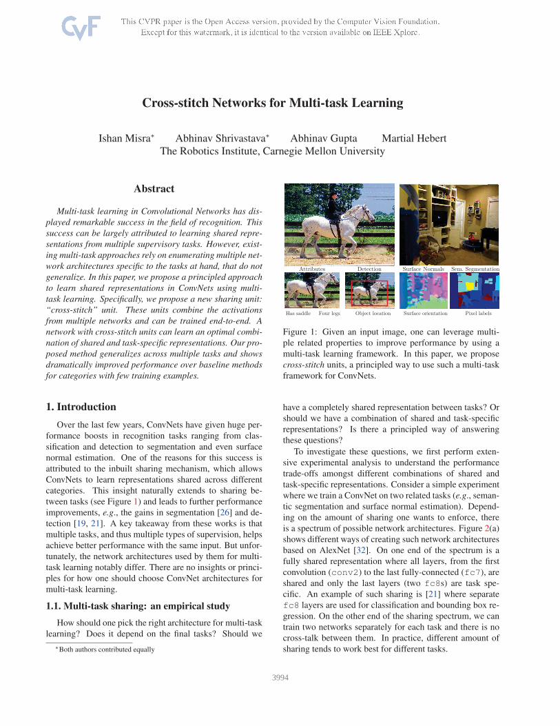
DetectionAttributes

Has saddle Four legs Object location

Surface Normals Sem. Segmentation

Surface orientation Pixel labels

Figure 1: Given an input image, one can leverage multi-

ple related properties to improve performance by using a

multi-task learning framework. In this paper, we propose

cross-stitch units, a principled way to use such a multi-task

framework for ConvNets.

have a completely shared representation between tasks? Or

should we have a combination of shared and task-specific

representations? Is there a principled way of answering

these questions?

To investigate these questions, we first perform exten-

sive experimental analysis to understand the performance

trade-offs amongst different combinations of shared and

task-specific representations. Consider a simple experiment

where we train a ConvNet on two related tasks (e.g., seman-

tic segmentation and surface normal estimation). Depend-

ing on the amount of sharing one wants to enforce, there

is a spectrum of possible network architectures. Figure 2(a)

shows different ways of creating such network architectures

based on AlexNet [32]. On one end of the spectrum is a

fully shared representation where all layers, from the first

convolution (conv2) to the last fully-connected (fc7), are

shared and only the last layers (two fc8s) are task spe-

cific. An example of such sharing is [21] where separate

fc8 layers are used for classification and bounding box re-

gression. On the other end of the sharing spectrum, we can

train two networks separately for each task and there is no

cross-talk between them. In practice, different amount of

sharing tends to work best for different tasks.

13994

-5.7

-2.2-1.2 -0.8 -1

-0.4

0.1

-0.16

0.69

-0.06 -0.09

0.37 0.24

-0.34

0.850.52 0.65

0.28

0.65 0.520.85

-0.4

0.11

-0.62

0.22

0.8

-0.28

-1.32

Figure 2: We train a variety of multi-task (two-task) architectures by splitting at different layers in a ConvNet [32] for two

pairs of tasks. For each of these networks, we plot their performance on each task relative to the task-specific network. We

notice that the best performing multi-task architecture depends on the individual tasks and does not transfer across different

pairs of tasks.

So given a pair of tasks, how should one pick a network

architecture? To empirically study this question, we pick

two varied pairs of tasks:

• We first pair semantic segmentation (SemSeg) and sur-

face normal prediction (SN). We believe the two tasks are

closely related to each other since segmentation bound-

aries also correspond to surface normal boundaries. For

this pair of tasks, we use NYU-v2 [47] dataset.

• For our second pair of tasks we use detection (Det) and

Attribute prediction (Attr). Again we believe that two

tasks are related: for example, a box labeled as “car”

would also be a positive example of “has wheel” at-

tribute. For this experiment, we use the attribute PAS-

CAL dataset [12, 16].

We exhaustively enumerate all the possible Split archi-

tectures as shown in Figure 2(a) for these two pairs of tasks

and show their respective performance in Figure 2(b). The

best performance for both the SemSeg and SN tasks is using

the “Split conv4” architecture (splitting at conv4), while

for the Det task it is using the Split conv2, and for Attr with

Split fc6. These results indicate two things – 1) Networks

learned in a multi-task fashion have an edge over networks

trained with one task; and 2) The best Split architecture for

multi-task learning depends on the tasks at hand.

While the gain from multi-task learning is encouraging,

getting the most out of it is still cumbersome in practice.

This is largely due to the task dependent nature of picking

architectures and the lack of a principled way of exploring

them. Additionally, enumerating all possible architectures

for each set of tasks is impractical. This paper proposes

cross-stitch units, using which a single network can capture

all these Split-architectures (and more). It automatically

learns an optimal combination of shared and task-specific

representations. We demonstrate that such a cross-stitched

network can achieve better performance than the networks

found by brute-force enumeration and search.

2. Related Work

Generic Multi-task learning [5, 48] has a rich history in

machine learning. The term multi-task learning (MTL) it-

self has been broadly used [2, 14, 28, 42, 54, 55] as an

umbrella term to include representation learning and se-

lection [4, 13, 31, 37], transfer learning [39, 41, 56] etc.

and their widespread applications in other fields, such as

genomics [38], natural language processing [7, 8, 35] and

computer vision [3, 10, 30, 31, 40, 51, 53, 58]. In fact, many

times multi-task learning is implicitly used without refer-

ence; a good example being fine-tuning or transfer learn-

ing [41], now a mainstay in computer vision, can be viewed

as sequential multi-task learning [5]. Given the broad scope,

in this section we focus only on multi-task learning in the

context of ConvNets used in computer vision.

Multi-task learning is generally used with ConvNets in

computer vision to model related tasks jointly, e.g. pose es-

timation and action recognition [22], surface normals and

edge labels [52], face landmark detection and face de-

tection [57, 59], auxiliary tasks in detection [21], related

3995

Shared

Task A

Shared

Task B

Cross-stitch unitInput

Activation Maps

Output

Activation Maps

Task A

Task B

Figure 3: We model shared representations by learning a

linear combination of input activation maps. At each layer

of the network, we learn such a linear combination of the

activation maps from both the tasks. The next layers’ filters

operate on this shared representation.

classes for image classification [50] etc. Usually these

methods share some features (layers in ConvNets) amongst

tasks and have some task-specific features. This sharing or

split-architecture (as explained in Section 1.1) is decided

after experimenting with splits at multiple layers and pick-

ing the best one. Of course, depending on the task at hand,

a different Split architecture tends to work best, and thus

given new tasks, new split architectures need to be explored.

In this paper, we propose cross-stitch units as a principled

approach to explore and embody such Split architectures,

without having to train all of them.

In order to demonstrate the robustness and effectiveness

of cross-stitch units in multi-task learning, we choose var-

ied tasks on multiple datasets. In particular, we select four

well established and diverse tasks on different types of im-

age datasets: 1) We pair semantic segmentation [27, 45, 46]

and surface normal estimation [11, 18, 52], both of which

require predictions over all pixels, on the NYU-v2 indoor

dataset [47]. These two tasks capture both semantic and

geometric information about the scene. 2) We choose

the task of object detection [17, 20, 21, 44] and attribute

prediction [1, 15, 33] on web-images from the PASCAL

dataset [12, 16]. These tasks make predictions about lo-

calized regions of an image.

3. Cross-stitch Networks

In this paper, we present a novel approach to multi-

task learning for ConvNets by proposing cross-stitch units.

Cross-stitch units try to find the best shared representations

for multi-task learning. They model these shared represen-

tations using linear combinations, and learn the optimal lin-

ear combinations for a given set of tasks. We integrate these

cross-stitch units into a ConvNet and provide an end-to-end

learning framework. We use detailed ablative studies to bet-

ter understand these units and their training procedure. Fur-

ther, we demonstrate the effectiveness of these units for two

different pairs of tasks. To limit the scope of this paper, we

only consider tasks which take the same single input, e.g.,

an image as opposed to say an image and a depth-map [25].

3.1. Split Architectures

Given a single input image with multiple labels, one can

design “Split architectures” as shown in Figure 2. These

architectures have both a shared representation and a task

specific representation. ‘Splitting’ a network at a lower

layer allows for more task-specific and fewer shared lay-

ers. One extreme of Split architectures is splitting at the

lowest convolution layer which results in two separate net-

works altogether, and thus only task-specific representa-

tions. The other extreme is using “sibling” prediction lay-

ers (as in [21]), which allows for a more shared representa-

tion. Thus, Split architectures allow for a varying amount

of shared and task-specific representations.

3.2. Unifying Split Architectures

Given that Split architectures hold promise for multi-task

learning, an obvious question is – At which layer of the

network should one split? This decision is highly dependent

on the input data and tasks at hand. Rather than enumerating

the possibilities of Split architectures for every new input

task, we propose a simple architecture that can learn how

much shared and task specific representation to use.

3.3. Cross-stitch units

Consider a case of multi task learning with two tasks Aand B on the same input image. For the sake of explanation,

consider two networks that have been trained separately for

these tasks. We propose a new unit, cross-stitch unit, that

combines these two networks into a multi-task network in

a way such that the tasks supervise how much sharing is

needed, as illustrated in Figure 3. At each layer of the net-

work, we model sharing of representations by learning a lin-

ear combination of the activation maps [4, 31] using a cross-

stitch unit. Given two activation maps xA, xB from layer

l for both the tasks, we learn linear combinations xA, xB

(Eq 1) of both the input activations and feed these combi-

nations as input to the next layers’ filters. This linear com-

bination is parameterized using α. Specifically, at location

(i, j) in the activation map,

⎡

⎣

xijA

xij

B

⎤

⎦ =

[

αAA αAB

αBA αBB

]

⎡

⎣

xijA

xij

B

⎤

⎦ (1)

We refer to this the cross-stitch operation, and the unit that

models it for each layer l as the cross-stitch unit. The net-

work can decide to make certain layers task specific by set-

ting αAB or αBA to zero, or choose a more shared represen-

tation by assigning a higher value to them.

3996

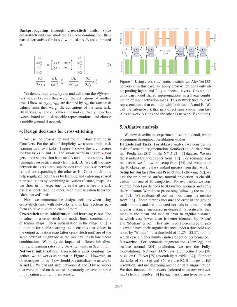
Backpropagating through cross-stitch units. Since

cross-stitch units are modeled as linear combination, their

partial derivatives for loss L with tasks A,B are computed

as

⎡

⎢

⎢

⎣

∂L

∂xij

A

∂L

∂xij

B

⎤

⎥

⎥

⎦

=

[

αAA αBA

αAB αBB

]

⎡

⎢

⎢

⎣

∂L

∂xij

A

∂L

∂xij

B

⎤

⎥

⎥

⎦

(2)

∂L

∂αAB

=∂L

∂xijB

xijA,

∂L

∂αAA

=∂L

∂xijA

xijA

(3)

We denote αAB, αBA by αD and call them the different-

task values because they weigh the activations of another

task. Likewise, αAA, αBB are denoted by αS, the same-task

values, since they weigh the activations of the same task.

By varying αD and αS values, the unit can freely move be-

tween shared and task-specific representations, and choose

a middle ground if needed.

4. Design decisions for cross-stitching

We use the cross-stitch unit for multi-task learning in

ConvNets. For the sake of simplicity, we assume multi-task

learning with two tasks. Figure 4 shows this architecture

for two tasks A and B. The sub-network in Figure 4(top)

gets direct supervision from task A and indirect supervision

(through cross-stitch units) from task B. We call the sub-

network that gets direct supervision from task A as network

A, and correspondingly the other as B. Cross-stitch units

help regularize both tasks by learning and enforcing shared

representations by combining activation (feature) maps. As

we show in our experiments, in the case where one task

has less labels than the other, such regularization helps the

“data-starved” tasks.

Next, we enumerate the design decisions when using

cross-stitch units with networks, and in later sections per-

form ablative studies on each of them.

Cross-stitch units initialization and learning rates: The

α values of a cross-stitch unit model linear combinations

of feature maps. Their initialization in the range [0, 1] is

important for stable learning, as it ensures that values in

the output activation map (after cross-stitch unit) are of the

same order of magnitude as the input values before linear

combination. We study the impact of different initializa-

tions and learning rates for cross-stitch units in Section 5.

Network initialization: Cross-stitch units combine to-

gether two networks as shown in Figure 4. However, an

obvious question is – how should one initialize the networks

A and B? We can initialize networks A and B by networks

that were trained on these tasks separately, or have the same

initialization and train them jointly.

conv1, pool1 conv2, pool2

Cross-stitch units

conv3 conv4 conv5, pool5 fc6 fc7 fc8

Task

AT

ask

B

Netw

ork

BN

etwork

AIm

age

Figure 4: Using cross-stitch units to stitch two AlexNet [32]

networks. In this case, we apply cross-stitch units only af-

ter pooling layers and fully connected layers. Cross-stitch

units can model shared representations as a linear combi-

nation of input activation maps. This network tries to learn

representations that can help with both tasks A and B. We

call the sub-network that gets direct supervision from task

A as network A (top) and the other as network B (bottom).

5. Ablative analysis

We now describe the experimental setup in detail, which

is common throughout the ablation studies.

Datasets and Tasks: For ablative analysis we consider the

tasks of semantic segmentation (SemSeg) and Surface Nor-

mal Prediction (SN) on the NYU-v2 [47] dataset. We use

the standard train/test splits from [18]. For semantic seg-

mentation, we follow the setup from [24] and evaluate on

the 40 classes using the standard metrics from their work

Setup for Surface Normal Prediction: Following [52], we

cast the problem of surface normal prediction as classifi-

cation into one of 20 categories. For evaluation, we con-

vert the model predictions to 3D surface normals and apply

the Manhattan-World post-processing following the method

in [52]. We evaluate all our methods using the metrics

from [18]. These metrics measure the error in the ground

truth normals and the predicted normals in terms of their

angular distance (measured in degrees). Specifically, they

measure the mean and median error in angular distance,

in which case lower error is better (denoted by ‘Mean’

and ‘Median’ error). They also report percentage of pix-

els which have their angular distance under a threshold (de-

noted by ‘Within t◦’ at a threshold of 11.25◦, 22.5◦, 30◦), in

which case a higher number indicates better performance.

Networks: For semantic segmentation (SemSeg) and

surface normal (SN) prediction, we use the Fully-

Convolutional Network (FCN 32-s) architecture from [36]

based on CaffeNet [29] (essentially AlexNet [32]). For both

the tasks of SemSeg and SN, we use RGB images at full

resolution, and use mirroring and color data augmentation.

We then finetune the network (referred to as one-task net-

work) from ImageNet [9] for each task using hyperparame-

3997

Table 1: Initializing cross-stitch units with different α val-

ues, each corresponding to a convex combination. Higher

values for αS indicate that we bias the cross-stitch unit to

prefer task specific representations. The cross-stitched net-

work is robust across different initializations of the units.

Surface Normal Segmentation

Angle Distance Within t◦

(Lower Better) (Higher Better) (Higher Better)

(αS, αD) Mean Med. 11.25 22.5 30 pixacc mIU fwIU

(0.1, 0.9) 34.6 18.8 38.5 53.7 59.4 47.9 18.2 33.3

(0.5, 0.5) 34.4 18.8 38.5 53.7 59.5 47.2 18.6 33.8

(0.7, 0.3) 34.0 18.3 38.9 54.3 60.1 48.0 18.6 33.6

(0.9, 0.1) 34.0 18.3 39.0 54.4 60.2 48.2 18.9 34.0

ters reported in [36]. We fine-tune the network for seman-

tic segmentation for 25k iterations using SGD (mini-batch

size 20) and for surface normal prediction for 15k iterations

(mini-batch size 20) as they gave the best performance, and

further training (up to 40k iterations) showed no improve-

ment. These one-task networks serve as our baselines and

initializations for cross-stitching, when applicable.

Cross-stitching: We combine two AlexNet architectures

using the cross-stitch units as shown in Figure 4. We ex-

perimented with applying cross-stitch units after every con-

volution activation map and after every pooling activation

map, and found the latter performed better. Thus, the cross-

stitch units for AlexNet are applied on the activation maps

for pool1, pool2, pool5, fc6 and fc7. We maintain

one cross-stitch unit per ‘channel’ of the activation map,

e.g., for pool1 we have 96 cross-stitch units.

5.1. Initializing parameters of cross-stitch units

Cross-stitch units capture the intuition that shared rep-

resentations can be modeled by linear combinations [31].

To ensure that values after the cross-stitch operation are of

the same order of magnitude as the input values, an obvious

initialization of the unit is that the α values form a con-

vex linear combination, i.e., the different-task αD and the

same-task αS to sum to one. Note that this convexity is

not enforced on the α values in either Equation 1 or 2, but

serves as a reasonable initialization. For this experiment,

we initialize the networks A and B with one-task networks

that were fine-tuned on the respective tasks. Table 1 shows

the results of evaluating cross-stitch networks for different

initializations of α values.

5.2. Learning rates for cross-stitch units

We initialize the α values of the cross-stitch units in the

range [0.1, 0.9], which is about one to two orders of mag-

nitude larger than the typical range of layer parameters in

AlexNet [32]. While training, we found that the gradient

updates at various layers had magnitudes which were rea-

Table 2: Scaling the learning rate of cross-stitch units wrt.

the base network. Since the cross-stitch units are initialized

in a different range from the layer parameters, we scale their

learning rate for better training.

Surface Normal Segmentation

Angle Distance Within t◦

(Lower Better) (Higher Better) (Higher Better)

Scale Mean Med. 11.25 22.5 30 pixacc mIU fwIU

1 34.6 18.9 38.4 53.7 59.4 47.7 18.6 33.5

10 34.5 18.8 38.5 53.8 59.5 47.8 18.7 33.5

102 34.0 18.3 39.0 54.4 60.2 48.0 18.9 33.8

103 34.1 18.2 39.2 54.4 60.2 47.2 19.3 34.0

sonable for updating the layer parameters, but too small for

the cross-stitch units. Thus, we use higher learning rates

for the cross-stitch units than the base network. In practice,

this leads to faster convergence and better performance. To

study the impact of different learning rates, we again use

a cross-stitched network initialized with two one-task net-

works. We scale the learning rates (wrt. the network’s learn-

ing rate) of cross-stitch units in powers of 10 (by setting the

lr mult layer parameter in Caffe [29]). Table 2 shows the

results of using different learning rates for the cross-stitch

units after training for 10k iterations. Setting a higher scale

for the learning rate improves performance, with the best

range for the scale being 102 − 103. We observed that set-

ting the scale to an even higher value made the loss diverge.

5.3. Initialization of networks A and B

When cross-stitching two networks, how should one ini-

tialize the networks A and B? Should one start with task

specific one-task networks (fine-tuned for one task only)

and add cross-stitch units? Or should one start with net-

works that have not been fine-tuned for the tasks? We

explore the effect of both choices by initializing using

two one-task networks and two networks trained on Im-

ageNet [9, 43]. We train the one-task initialized cross-

stitched network for 10k iterations and the ImageNet ini-

tialized cross-stitched network for 30k iterations (to account

for the 20k fine-tuning iterations of the one-task networks),

and report the results in Table 3. Task-specific initializa-

tion performs better than ImageNet initialization for both

the tasks, which suggests that cross-stitching should be used

after training task-specific networks.

5.4. Visualization of learned combinations

We visualize the weights αS and αD of the cross-stitch

units for different initializations in Figure 4. For this exper-

iment, we initialize sub-networks A and B using one-task

networks and trained the cross-stitched network till con-

vergence. Each plot shows (in sorted order) the α values

for all the cross-stitch units in a layer (one per channel).

3998

Table 3: We initialize the networks A, B (from Figure 4)

from ImageNet, as well as task-specific networks. We

observe that task-based initialization performs better than

task-agnostic ImageNet initialization.

Surface Normal Segmentation

Angle Distance Within t◦

(Lower Better) (Higher Better) (Higher Better)

Init. Mean Med. 11.25 22.5 30 pixacc mIU fwIU

ImageNet 34.6 18.8 38.6 53.7 59.4 48.0 17.7 33.4

One-task 34.1 18.2 39.0 54.4 60.2 47.2 19.3 34.0

We show plots for three layers: pool1, pool5 and fc7.

The initialization of cross-stitch units biases the network to

start its training preferring a certain type of shared repre-

sentation, e.g., (αS, αD) = (0.9, 0.1) biases the network

to learn more task-specific features, while (0.5, 0.5) biases

it to share representations. Figure 4 (second row) shows

that both the tasks, across all initializations, prefer a more

task-specific representation for pool5, as shown by higher

values of αS. This is inline with the observation from Sec-

tion 1.1 that Split conv4 performs best for these two tasks.

We also notice that the surface normal task prefers shared

representations as can be seen by Figure 4(b), where αS and

αD values are in similar range.

6. Experiments

We now present experiments with cross-stitch networks

for two pairs of tasks: semantic segmentation and surface

normal prediction on NYU-v2 [47], and object detection

and attribute prediction on PASCAL VOC 2008 [12, 16].

We use the experimental setup from Section 5 for semantic

segmentation and surface normal prediction, and describe

the setup for detection and attribute prediction below.

Dataset, Metrics and Network: We consider the PAS-

CAL VOC 20 classes for object detection, and the 64 at-

tribute categories data from [16]. We use the PASCAL VOC

2008 [12, 16] dataset for our experiments and report results

using the standard Average Precision (AP) metric. We start

with the recent Fast-RCNN [21] method for object detection

using the AlexNet [32] architecture.

Training: For object detection, Fast-RCNN is trained us-

ing 21-way 1-vs-all classification with 20 foreground and 1

background class. However, there is a severe data imbal-

ance in the foreground and background data points (boxes).

To circumvent this, Fast-RCNN carefully constructs mini-

batches with 1 : 3 foreground-to-background ratio, i.e.,

at most 25% of foreground samples in a mini-batch. At-

tribute prediction, on the other hand, is a multi-label classi-

fication problem with 64 attributes, which only train using

foreground bounding boxes. To implement both tasks in

the Fast R-CNN framework, we use the same mini-batch

sampling strategy; and in every mini-batch only the fore-

ground samples contribute to the attribute loss (and back-

ground samples are ignored).

Scaling losses: Both SemSeg and SN used same classifi-

cation loss for training, and hence we were set their loss

weights to be equal (= 1). However, since object detection

is formulated as 1-vs-all classification and attribute classi-

fication as multi-label classification, we balance the losses

by scaling the attribute loss by 1/64.

Cross-stitching: We combine two AlexNet architectures

using the cross-stitch units after every pooling layer as

shown in Figure 4. In the case of object detection and at-

tribute prediction, we use one cross-stitch unit per layer ac-

tivation map. We found that maintaining a unit per channel,

like in the case of semantic segmentation, led to unstable

learning for these tasks.

6.1. Baselines

We compare against four strong baselines for the two

pairs of tasks and report the results in Table 5 and 6.

Single-task Baselines: These serve as baselines without

benefits of multi-task learning. First we evaluate a single

network trained on only one task (denoted by ‘One-task’)

as described in Section 5. Since our approach cross-stitches

two networks and therefore uses 2× parameters, we also

consider an ensemble of two one-task networks (denoted

by ‘Ensemble’). However, note that the ensemble has 2×network parameters for only one task, while the cross-stitch

network has roughly 2× parameters for two tasks. So for a

pair of tasks, the ensemble baseline uses ∼ 2× the cross-

stitch parameters.

Multi-task Baselines: The cross-stitch units enable the net-

work to pick an optimal combination of shared and task-

specific representation. We demonstrate that these units re-

move the need for finding such a combination by exhaustive

brute-force search (from Section 1.1). So as a baseline, we

train all possible “Split architectures” for each pair of tasks

and report numbers for the best Split for each pair of tasks.

There has been extensive work in Multi-task learning

outside of the computer vision and deep learning commu-

nity. However, most of such work, with publicly avail-

able code, formulates multi-task learning in an optimiza-

tion framework that requires all data points in memory [6,

14, 23, 34, 49, 60, 61]. Such requirement is not practical for

the vision tasks we consider.

So as our final baseline, we compare to a variant of [1,

62] by adapting their method to our setting and report this

as ‘MTL-shared’. The original method treats each cate-

gory as a separate ‘task’, a separate network is required

for each category and all these networks are trained jointly.

Directly applied to our setting, this would require training

100s of ConvNets jointly, which is impractical. Thus, in-

stead of treating each category as an independent task, we

3999

Table 4: We show the sorted α values (increasing left to right) for three layers. A higher value of αS indicates a strong pref-

erence towards task specific features, and a higher αD implies preference for shared representations. More detailed analysis

in Section 5.4. Note that both αS and αD are sorted independently, so the channel-index across them do not correspond.

Layer (a) αS = 0.9, αD = 0.1 (b) αS = 0.5, αD = 0.5 (c) αS = 0.1, αD = 0.9

Segmentation Surface Normal Segmentation Surface Normal Segmentation Surface Normal

pool1

pool5

fc7

Lea

the

r

Ho

rn

Sa

il

Pro

pe

lle

r

Sa

dd

le

Flo

we

r

Ma

st

Ro

un

d

En

gin

e

Je

t e

ng

ine

Cle

ar

Re

in

Ste

m/T

run

k

Pe

da

l

Wo

ol

Scr

ee

n

Exh

au

st

La

be

l

Po

t

Le

af

Be

ak

Ve

ge

tati

on

Te

xt

Ro

w W

ind

Fu

rn.

Arm

Ha

nd

leb

ars

Ta

illi

gh

t

Fe

ath

er

Ho

riz

Cy

l

Fu

rn.

Leg

Win

g

Sid

e m

irro

r

Fu

rn.

Se

at

He

ad

lig

ht

Do

or

Wo

od

2D

Bo

xy

Gla

ss

Ve

rt C

yl

Fu

rn.

Ba

ck

Ta

il

Pla

stic

Sn

ou

t

Fu

rry

Win

do

w

Wh

ee

l

3D

Bo

xy

Sh

iny

Fo

ot/

Sh

oe

Ha

nd

Me

tal

Mo

uth

No

se

Fa

ce

Ha

ir

Arm Ea

r

Le

g

Ey

e

Sk

in

Clo

th

To

rso

He

ad

Occ

lud

ed

Figure 5: Change in performance for attribute categories over the baseline is indicated by blue bars. We sort the categories

in increasing order (from left to right) by the number of instance labels in the train set, and indicate the number of instance

labels by the solid black line. The performance gain for attributes with lesser data (towards the left) is considerably higher

compared to the baseline. We also notice that the gain for categories with lots of data is smaller.

adapt their method to our two-task setting. We train these

two networks jointly, using end-to-end learning, as opposed

to their dual optimization to reduce hyperparameter search.

6.2. Semantic Segmentation and Surface NormalPrediction

Table 5 shows the results for semantic segmentation and

surface normal prediction on the NYUv2 dataset [47]. We

compare against two one-task networks, an ensemble of two

networks, and the best Split architecture (found using brute

force enumeration). The sub-networks A, B (Figure 4)

in our cross-stitched network are initialized from the one-

task networks. We use cross-stitch units after every pool-

ing layer and fully connected layer (one per channel). Our

proposed cross-stitched network improves results over the

baseline one-task networks and the ensemble. Note that

even though the ensemble has 2× parameters compared to

cross-stitched network, the latter performs better. Finally,

our performance is better than the best Split architecture

network found using brute force search. This shows that the

cross-stitch units can effectively search for optimal amount

of sharing in multi-task networks.

6.3. Data-starved categories for segmentation

Multiple tasks are particularly helpful in regularizing the

learning of shared representations[5, 14, 50]. This regular-

ization manifests itself empirically in the improvement of

“data-starved” (few examples) categories and tasks.

For semantic segmentation, there is a high mismatch in

the number of labels per category (see the black line in Fig-

4000

Table 5: Surface normal prediction and semantic segmenta-

tion results on the NYU-v2 [47] dataset. Our method out-

performs the baselines for both the tasks.

Surface Normal Segmentation

Angle Distance Within t◦

(Lower Better) (Higher Better) (Higher Better)

Method Mean Med. 11.25 22.5 30 pixacc mIU fwIU

One-task34.8 19.0 38.3 53.5 59.2 - - -

- - - - - 46.6 18.4 33.1

Ensemble34.4 18.5 38.7 54.2 59.7 - - -

- - - - - 48.2 18.9 33.8

Split conv4 34.7 19.1 38.2 53.4 59.2 47.8 19.2 33.8

MTL-shared 34.7 18.9 37.7 53.5 58.8 45.9 16.6 30.1

Cross-stitch [ours] 34.1 18.2 39.0 54.4 60.2 47.2 19.3 34.0

bag

bathtub

whiteboard

sink

night-stand

lamp

person

toilet

towel

shower-curtain

paper

box

refridgerator

books

television

floor-mat

ceiling

curtain

clothes

pillow

mirror

dresser

desk

shelves

blinds

counter

picture

door

bookshelf

window

otherfurniture

otherstructure

table

sofa

bed

chair

otherprop

cabinet

floor

wall

Figure 6: Change in performance (meanIU metric) for se-

mantic segmentation categories over the baseline is indi-

cated by blue bars. We sort the categories (in increasing

order from left to right) by the number of pixel labels in

the train set, and indicate the number of pixel labels by a

solid black line. The performance gain for categories with

lesser data (towards the left) is more when compared to the

baseline one-task network.

ure 6). Some classes like wall, floor have many more in-

stances than other classes like bag, whiteboard etc. Fig-

ure 6 also shows the per-class gain in performance using

our method over the baseline one-task network. We see that

cross-stitch units considerably improve the performance of

“data-starved” categories (e.g., bag, whiteboard).

6.4. Object detection and attribute prediction

We train a cross-stitch network for the tasks of object de-

tection and attribute prediction. We compare against base-

line one-task networks and the best split architectures per

task (found after enumeration and search, Section 1.1). Ta-

ble 6 shows the results for object detection and attribute pre-

diction on PASCAL VOC 2008 [12, 16]. Our method shows

improvements over the baseline for attribute prediction. It

is worth noting that because we use a background class for

detection, and not attributes (described in ‘Scaling losses’

in Section 6), detection has many more data points than at-

tribute classification (only 25% of a mini-batch has attribute

labels). Thus, we see an improvement for the data-starved

Table 6: Object detection and attribute prediction results on

the attribute PASCAL [16] 2008 dataset

Method Detection (mAP) Attributes (mAP)

One-task44.9 -

- 60.9

Ensemble46.1 -

- 61.1

Split conv2 44.6 61.0

Split fc7 44.8 59.7

MTL-shared 42.7 54.1

Cross-stitch [ours] 45.2 63.0

task of attribute prediction. It is also interesting to note that

the detection task prefers a shared representation (best per-

formance by Split fc7), whereas the attribute task prefers a

task-specific network (best performance by Split conv2).

6.5. Data-starved categories for attribute prediction

Following a similar analysis to Section 6.3, we plot the

relative performance of our cross-stitch approach over the

baseline one-task attribute prediction network in Figure 5.

The performance gain for attributes with smaller number

of training examples is considerably large compared to the

baseline (4.6% and 4.3% mAP for the top 10 and 20 at-

tributes with the least data respectively). This shows that

our proposed cross-stitch method provides significant gains

for data-starved tasks by learning shared representations.

7. Conclusion

We present cross-stitch units which are a generalized

way of learning shared representations for multi-task learn-

ing in ConvNets. Cross-stitch units model shared represen-

tations as linear combinations, and can be learned end-to-

end in a ConvNet. These units generalize across different

types of tasks and eliminate the need to search through sev-

eral multi-task network architectures on a per task basis. We

show detailed ablative experiments to see effects of hyper-

parameters, initialization etc. when using these units. We

also show considerable gains over the baseline methods for

data-starved categories. Studying other properties of cross-

stitch units, such as where in the network should they be

used and how should their weights be constrained, is an in-

teresting future direction.

Acknowledgments: We would like to thank Alyosha Efros

and Carl Doersch for helpful discussions. This work was sup-

ported in part by ONR MURI N000141612007 and the US Army

Research Laboratory (ARL) under the CTA program (Agreement

W911NF-10-2-0016). AS was supported by the MSR fellowship.

We thank NVIDIA for donating GPUs.

4001

References

[1] A. H. Abdulnabi, G. Wang, J. Lu, and K. Jia. Multi-task

CNN model for attribute prediction. IEEE Multimedia, 17,

2015. 3, 6[2] Y. Amit, M. Fink, N. Srebro, and S. Ullman. Uncovering

shared structures in multiclass classification. In ICML, 2007.

2[3] V. S. Anastasia Pentina and C. H. Lampert. Curriculum

learning of multiple tasks. In CVPR, 2015. 2[4] A. Argyriou, T. Evgeniou, and M. Pontil. Convex multi-task

feature learning. JMLR, 73, 2008. 2, 3[5] R. Caruana. Multitask learning. Machine learning, 28, 1997.

2, 7[6] J. Chen, J. Zhou, and J. Ye. Integrating low-rank and group-

sparse structures for robust multi-task learning. In SIGKDD,

2011. 6[7] R. Collobert and J. Weston. A unified architecture for natural

language processing: Deep neural networks with multitask

learning. In ICML, 2008. 2[8] R. Collobert, J. Weston, L. Bottou, M. Karlen,

K. Kavukcuoglu, and P. Kuksa. Natural language pro-

cessing (almost) from scratch. JMLR, 12, 2011. 2[9] J. Deng, W. Dong, R. Socher, L. jia Li, K. Li, and L. Fei-

fei. Imagenet: A large-scale hierarchical image database. In

CVPR, 2009. 4, 5[10] J. Donahue, Y. Jia, O. Vinyals, J. Hoffman, N. Zhang,

E. Tzeng, and T. Darrell. Decaf: A deep convolutional acti-

vation feature for generic visual recognition. arXiv preprint

arXiv:1310.1531, 2013. 2[11] D. Eigen and R. Fergus. Predicting depth, surface normals

and semantic labels with a common multi-scale convolu-

tional architecture. In ICCV, 2015. 3[12] M. Everingham, L. Van Gool, C. K. I. Williams, J. Winn, and

A. Zisserman. The PASCAL Visual Object Classes Chal-

lenge 2007 (VOC2007). 2, 3, 6, 8[13] A. Evgeniou and M. Pontil. Multi-task feature learning.

NIPS, 19:41, 2007. 2[14] T. Evgeniou and M. Pontil. Regularized multi–task learning.

In SIGKDD, 2004. 2, 6, 7[15] A. Farhadi, I. Endres, and D. Hoiem. Attribute-centric recog-

nition for cross-category generalization. In CVPR, 2010. 3[16] A. Farhadi, I. Endres, D. Hoiem, and D. Forsyth. Describing

objects by their attributes. In CVPR, 2009. 2, 3, 6, 8[17] P. Felzenszwalb, R. Girshick, D. McAllester, and D. Ra-

manan. Object detection with discriminatively trained part-

based models. PAMI, 2010. 3[18] D. F. Fouhey, A. Gupta, and M. Hebert. Data-driven 3D

primitives for single image understanding. In ICCV, 2013.

3, 4[19] S. Gidaris and N. Komodakis. Object detection via a multi-

region & semantic segmentation-aware cnn model. arXiv

preprint arXiv:1505.01749, 2015. 1[20] R. Girshick, J. Donahue, T. Darrell, and J. Malik. Rich fea-

ture hierarchies for accurate object detection and semantic

segmentation. In CVPR, 2014. 3[21] R. B. Girshick. Fast R-CNN. In ICCV, 2015. 1, 2, 3, 6[22] G. Gkioxari, B. Hariharan, R. Girshick, and J. Malik. R-

cnns for pose estimation and action detection. arXiv preprint

arXiv:1406.5212, 2014. 2

[23] Q. Gu and J. Zhou. Learning the shared subspace for multi-

task clustering and transductive transfer classification. In

ICDM, 2009. 6[24] S. Gupta, P. Arbelaez, and J. Malik. Perceptual organiza-

tion and recognition of indoor scenes from rgb-d images. In

CVPR, 2013. 4[25] S. Gupta, R. Girshick, P. Arbelaez, and J. Malik. Learning

rich features from rgb-d images for object detection and seg-

mentation. In ECCV, 2014. 3[26] B. Hariharan, P. Arbelaez, R. Girshick, and J. Malik. Si-

multaneous detection and segmentation. In ECCV. Springer,

2014. 1[27] G. Heitz and D. Koller. Learning spatial context: Using stuff

to find things. In ECCV. 2008. 3[28] A. Jalali, S. Sanghavi, C. Ruan, and P. K. Ravikumar. A dirty

model for multi-task learning. In NIPS, 2010. 2[29] Y. Jia, E. Shelhamer, J. Donahue, S. Karayev, J. Long, R. Gir-

shick, S. Guadarrama, and T. Darrell. Caffe: Convolutional

architecture for fast feature embedding. In ACMM, 2014. 4,

5[30] J. Y. H. Jung, B. Yoo, C. Choi, D. Park, and J. Kim. Rotating

your face using multi-task deep neural network. In CVPR,

2015. 2[31] Z. Kang, K. Grauman, and F. Sha. Learning with whom to

share in multi-task feature learning. In ICML, 2011. 2, 3, 5[32] A. Krizhevsky, I. Sutskever, and G. E. Hinton. Imagenet

classification with deep convolutional neural networks. In

NIPS, 2012. 1, 2, 4, 5, 6[33] C. H. Lampert, H. Nickisch, and S. Harmeling. Learning to

detect unseen object classes by between-class attribute trans-

fer. In CVPR, 2009. 3[34] M. Lapin, B. Schiele, and M. Hein. Scalable multitask rep-

resentation learning for scene classification. In CVPR, 2014.

6[35] X. Liu, J. Gao, X. He, L. Deng, K. Duh, and Y.-Y. Wang.

Representation learning using multi-task deep neural net-

works for semantic classification and information retrieval.

NAACL, 2015. 2[36] J. Long, E. Shelhamer, and T. Darrell. Fully convolu-

tional networks for semantic segmentation. arXiv preprint

arXiv:1411.4038, 2014. 4, 5[37] G. Obozinski, B. Taskar, and M. Jordan. Multi-task feature

selection. Statistics Department, UC Berkeley, Tech. Rep,

2006. 2[38] G. Obozinski, B. Taskar, and M. I. Jordan. Joint covariate

selection and joint subspace selection for multiple classifica-

tion problems. Statistics and Computing, 20, 2010. 2[39] S. J. Pan and Q. Yang. A survey on transfer learning.

Knowledge and Data Engineering, IEEE Transactions on,

22(10):1345–1359, 2010. 2[40] A. Quattoni, M. Collins, and T. Darrell. Transfer learning for

image classification with sparse prototype representations. In

CVPR, 2008. 2[41] A. S. Razavian, H. Azizpour, J. Sullivan, and S. Carls-

son. CNN features off-the-shelf: an astounding baseline for

recognition. In CVPR Workshop, 2014. 2[42] B. Romera-Paredes, A. Argyriou, N. Berthouze, and M. Pon-

til. Exploiting unrelated tasks in multi-task learning. In

ICAIS, 2012. 2[43] O. Russakovsky, J. Deng, H. Su, J. Krause, S. Satheesh,

4002

S. Ma, Z. Huang, A. Karpathy, A. Khosla, M. Bernstein,

A. C. Berg, and L. Fei-Fei. ImageNet Large Scale Visual

Recognition Challenge. IJCV, 115, 2015. 5[44] H. Schneiderman and T. Kanade. Object detection using the

statistics of parts. IJCV, 56, 2004. 3[45] J. Shi and J. Malik. Normalized cuts and image segmenta-

tion. TPAMI, 22, 2000. 3[46] J. Shotton, J. Winn, C. Rother, and A. Criminisi. Texton-

boost: Joint appearance, shape and context modeling for

multi-class object recognition and segmentation. In ECCV.

2006. 3[47] N. Silberman, D. Hoiem, P. Kohli, and R. Fergus. Indoor

segmentation and support inference from rgbd images. In

ECCV, 2012. 2, 3, 4, 6, 7, 8[48] C. Stein et al. Inadmissibility of the usual estimator for the

mean of a multivariate normal distribution. In Proceedings

of the Third Berkeley symposium on mathematical statistics

and probability, volume 1. 1956. 2[49] C. Su et al. Multi-task learning with low rank attribute em-

bedding for person re-identification. In ICCV, 2015. 6[50] P. Teterwak and L. Torresani. Shared Roots: Regularizing

Deep Neural Networks through Multitask Learning. Techni-

cal Report TR2014-762, Dartmouth College, Computer Sci-

ence, 2014. 3, 7[51] A. Torralba, K. P. Murphy, and W. T. Freeman. Sharing vi-

sual features for multiclass and multiview object detection.

PAMI, 29, 2007. 2[52] X. Wang, D. F. Fouhey, and A. Gupta. Designing deep net-

works for surface normal estimation. In CVPR, 2015. 2, 3,

4[53] J. Wright, Y. Ma, J. Mairal, G. Sapiro, T. S. Huang, and

S. Yan. Sparse representation for computer vision and pat-

tern recognition. Proceedings of the IEEE, 98(6):1031–1044,

2010. 2[54] Y. Xue, X. Liao, L. Carin, and B. Krishnapuram. Multi-

task learning for classification with dirichlet process priors.

JMLR, 8, 2007. 2[55] Y. Yang and T. M. Hospedales. A unified perspective

on multi-domain and multi-task learning. arXiv preprint

arXiv:1412.7489, 2014. 2[56] J. Yosinski, J. Clune, Y. Bengio, and H. Lipson. How trans-

ferable are features in deep neural networks? In NIPS, 2014.

2[57] C. Zhang and Z. Zhang. Improving multiview face detection

with multi-task deep convolutional neural networks. In Ap-

plications of Computer Vision (WACV), 2014 IEEE Winter

Conference on, pages 1036–1041. IEEE, 2014. 2[58] T. Zhang, B. Ghanem, S. Liu, and N. Ahuja. Robust visual

tracking via structured multi-task sparse learning. Interna-

tional journal of computer vision, 101(2):367–383, 2013. 2[59] Z. Zhang, P. Luo, C. C. Loy, and X. Tang. Facial landmark

detection by deep multi-task learning. In Computer Vision–

ECCV 2014, pages 94–108. Springer, 2014. 2[60] J. Zhou, J. Chen, and J. Ye. MALSAR: Multi-tAsk Learning

via StructurAl Regularization. ASU, 2011. 6[61] J. Zhou, J. Liu, V. A. Narayan, and J. Ye. Modeling disease

progression via fused sparse group lasso. In SIGKDD, 2012.

6[62] Q. Zhou, G. Wang, K. Jia, and Q. Zhao. Learning to share

latent tasks for action recognition. In ICCV, 2013. 6

4003