cross-sectional phenomena and cedric ehouarne
TRANSCRIPT

CROSS-SECTIONAL PHENOMENA ANDNEW PERSPECTIVES ON MACRO-FINANCE PUZZLES
Cedric Ehouarne
Dissertation Submitted in Partial Fulfillmentof the Requirements for the Degree of
DOCTOR OF PHILOSOPHY
CommitteeLars-Alexander Kuehn (chair)
Sevin YeltekinAriel Zetlin-Jones
Daniele Coen-Pirani
April 2016
Dedicated to my lovely wife Anne-Sophie Perrin
and my dear father Michel Ehouarne
Abstract
Traditional models of the business cycle rely on the assumption that the economy
is populated by agents who have similar characteristics such as taste income or pro-
ductivity Despite offering simple and elegant macroeconomic models this assumption
masks the rich interplay between cross-sectional and aggregate cyclical movements The
goal of this dissertation is to show in two distinct contexts of heterogeneity ndash households
and firms ndash how such interplay can shed new light on classic puzzles in the macro-finance
literature such as the high volatility of unemployment or the large equity premium
The first chapter titled ldquoThe Macroeconomics of Consumer Financerdquo studies the
macroeconomic effects of consumer credit conditions in an incomplete-market general
equilibrium model where households hold unsecured debt and firms use labor I show
that consumer finance disturbances can cause business cycle fluctuations through a rich
interplay between credit and labor risks As unemployment rises households are more
likely to default translating into tighter credit conditions that reduce their consumption
and cause further unemployment Such feedback loop is reinforced by precautionary-
saving motives among unconstrained households Surprisingly this mechanism can
explain a large fraction of the volatility and persistence of US unemployment even
though it abstracts from traditional frictions like search or price stickiness
In the second chapter titled ldquoMisallocation Cyclesrdquo and co-authored with Lars-
Alexander Kuehn and David Schreindorfer we estimate a general equilibrium model
with firm heterogeneity and a representative household with Epstein-Zin preferences
Firms face investment frictions and permanent shocks which feature time-variation in
common idiosyncratic skewness Quantitatively the model replicates well the cyclical
dynamics of the cross-sectional output growth and investment rate distributions Eco-
nomically the model is able to generate business cycles through inefficiencies in the
allocation of capital across firms These cycles arise because (i) permanent Gaussian
shocks give rise to a power law distribution in firm size and (ii) rare negative Poisson
shocks cause time-variation in common idiosyncratic skewness
Acknowledgements
I am grateful to my advisor co-author and mentor Lars-Alexander Kuehn for his
support and guidance all along this project He has given me the freedom to think
outside of the box and has guided me through my trials and errors with a lot of patience
His sense of humor and good mood made this journey extremely pleasant I am also
thankful to have David Schreindorfer as a co-author who is a bright and friendly scholar
I am deeply in debt of my advisors Sevin Yeltekin and Ariel Zetlin-Jones for their
incredible support and guidance They shared with me invaluable insights into my job
market paper and the whole job search process I am also grateful for the many years
I worked for Sevin as a Teaching Assistant for my favorite class ldquoGlobal Economicsrdquo
For helpful comments and suggestions on this dissertation and in particular on the
first chapter (my job market paper) I would like to thank Bryan R Routledge Brent
Glover Burton Hollifield Benjamin J Tengelsen and seminar participants at Carnegie
Mellon University HEC Montreal Universite du Quebec a Montreal Concordia Univer-
sity Universite Laval Bank of Canada and the Federal Reserve Board of Governors I
also would like to thank Daniele Coen-Pirani for serving on my committee I also thank
Lawrence Rapp for his help at the early stage of the job market process and for setting
such a good mood in the PhD lounge
For inspiring me to pursue a PhD I would like to thank my masterrsquos thesis advisor
Stephane Pallage and his wonderful colleagues at Universite du Quebec a Montreal
Finally I would like to thank my family and friends for supporting me during my
ups and downs during this long journey I dedicate this dissertation to my wife Anne-
Sophie Perrin for giving me the strength to accomplish this great achievement and my
father Michel Ehouarne for having always believed in me
List of Figures
11 Steady-State Policy Functions by Household Type 18
12 Steady-State Excess Demand in the Goods Market 21
13 Model-based Stationary Distributions by Household Type 27
14 Unemployment and Consumer Finance Statistics over the US
Business Cycle 29
15 Cross sectional moments of credit balances and limits as of
annual income 30
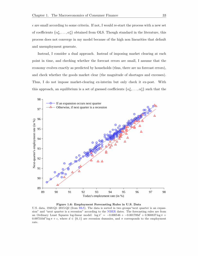
16 Employment Forecasting Rules in US Data 33
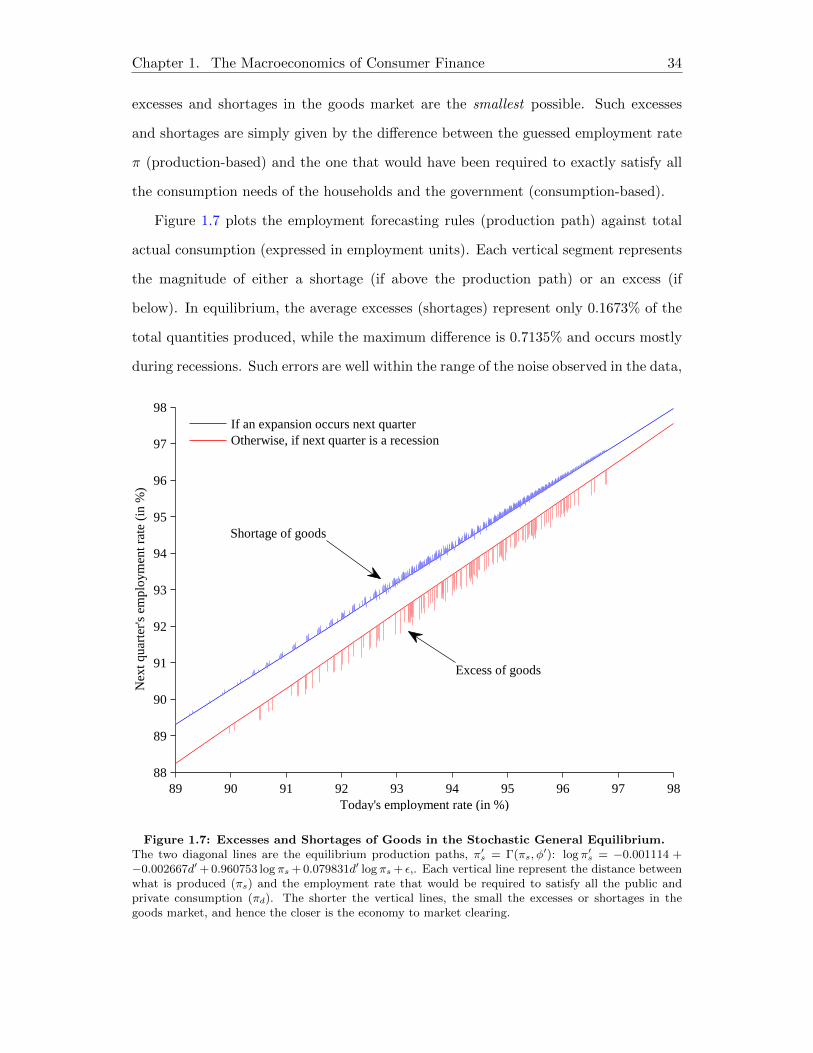
17 Excesses and Shortages of Goods in the Stochastic General
Equilibrium 34
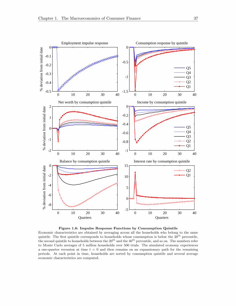
18 Impulse Response Functions by Consumption Quintile 37
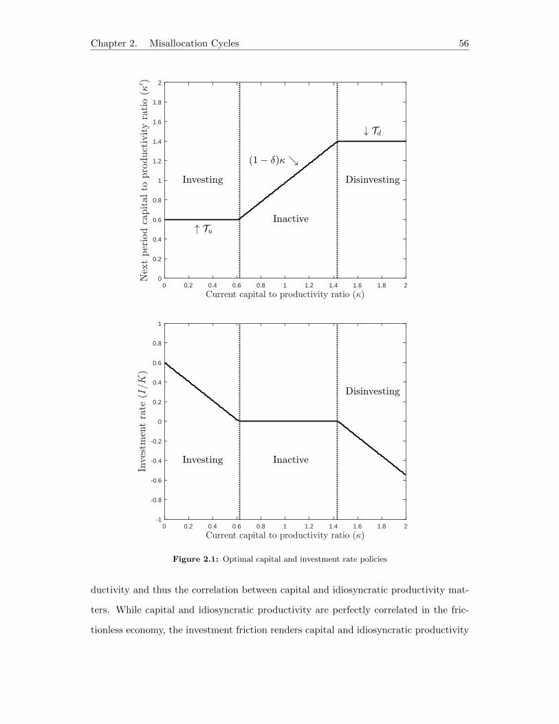
21 Optimal capital and investment rate policies 56
22 Optimal capital policies in the micro-distribution 58
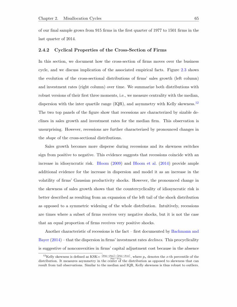
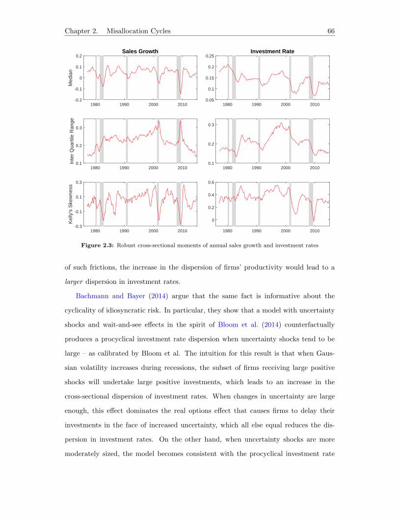
23 Robust cross-sectional moments of annual sales growth and investment
rates 66
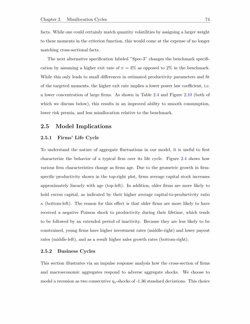
24 Life Cycle of a Firm Average Behavior and Quartiles 75
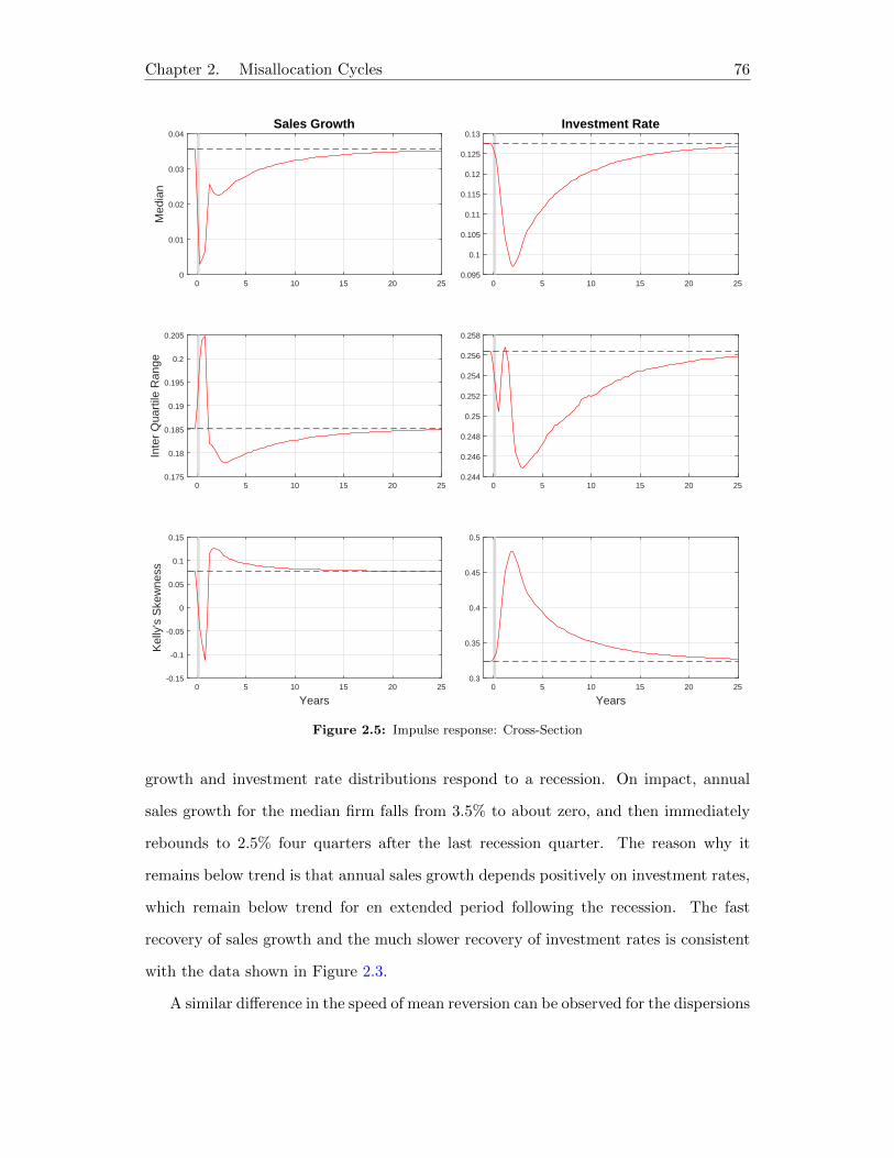
25 Impulse response Cross-Section 76
26 Impulse response Aggregates 78
27 Cross-Sectional Impulses by Firmsrsquo κ 79
28 Cross-Sectional Impulses by Firm Size 81
29 Output Concentration 82
210 Comparative statics for the exit rate 83
v
List of Tables
11 Model Statistics by Category of Borrowers 17
12 Model Parameter Values 22
13 Simulated and Actual Moments in Steady State 24
14 Alternative Steady-State Estimation without Preference Het-
erogeneity 26
15 OLS Coefficients of the Conditional Employment Forecasting
Rules 32
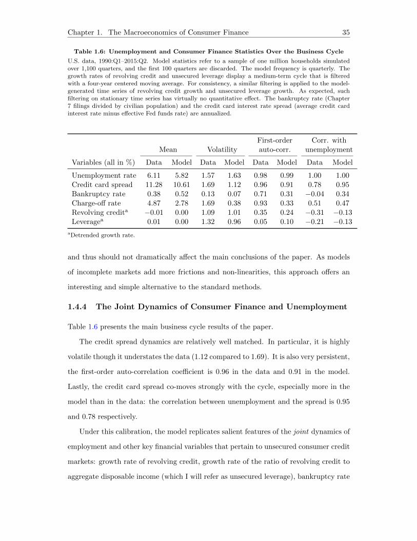
16 Unemployment and Consumer Finance Statistics Over the Busi-
ness Cycle 35
17 Household Economic Characteristics by Consumption Quintile
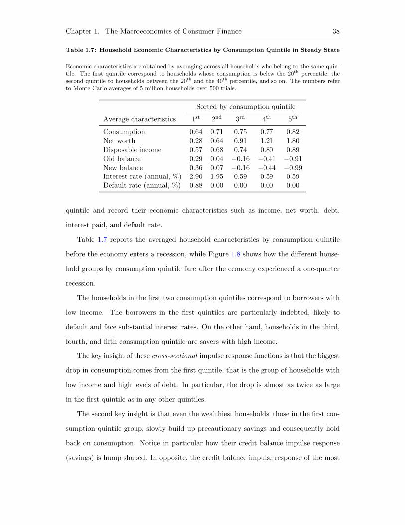
in Steady State 38
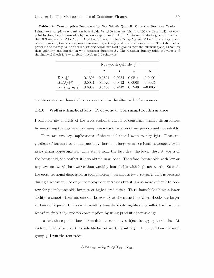
18 Consumption Insurance by Net Worth Quintile Over the Busi-
ness Cycle 39
21 Two stylized firm-level distributions 60
22 Predefined and Estimated Parameter Values 68
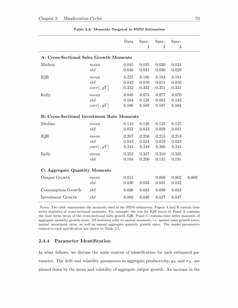
23 Moments Targeted in SMM Estimation 70
24 Consumption Growth and Asset Prices 73
vi
Contents
1 The Macroeconomics of Consumer Finance 1
11 Introduction 1
111 Literature 6
12 Modeling Consumer Finance and Systemic Risk 7
121 The Environment 8
122 Householdrsquos Problem 10
123 Bond Pricing 11
124 Aggregate Resources 11
125 General Equilibrium 12
126 Steady State 13
127 Solution Method 13
13 Estimating the Model Steady State 14
131 The Data 15
132 Mapping the Model to US Data 16
133 Identifying Preference Heterogeneity in the Data 18
134 Matching Moments 19
135 Results 20
136 Counterfactual Results without Preference Heterogeneity 25
137 Understanding the Role of Preference Heterogeneity 25
14 On the Cyclical Effects of Consumer Finance 28
141 Stylized Facts of the Cyclical Nature of Consumer Finance 28
142 Calibrating the Aggregate Financial Shock 31
143 Approximate Aggregation in the Model and in US Data 32
144 The Joint Dynamics of Consumer Finance and Unemployment 35
145 The Mechanism at Play From Cross-Sectionial to Aggregate 36
146 Welfare Implications Procyclical Consumption Insurance 39
147 Discussion 40
15 Conclusion 41
vii
2 Misallocation Cycles 43
21 Introduction 43
22 Model 47
221 Production 47
222 Firms 50
223 Household 51
224 Equilibrium 52
23 Analysis 52
231 Household Optimization 52
232 Firm Optimization 53
233 Aggregation 55
234 Frictionless Economy 59
235 Numerical Method 61
24 Estimation 63
241 Data 64
242 Cyclical Properties of the Cross-Section of Firms 65
243 Simulated Method of Moments 67
244 Parameter Identification 70
245 Baseline Estimates 72
246 Alternative Specifications 73
25 Model Implications 74
251 Firmsrsquo Life Cycle 74
252 Business Cycles 74
253 Power Law and Consumption Dynamics 81
26 Conclusion 84
A Computational Appendix 85
A1 Value Function Iteration 85
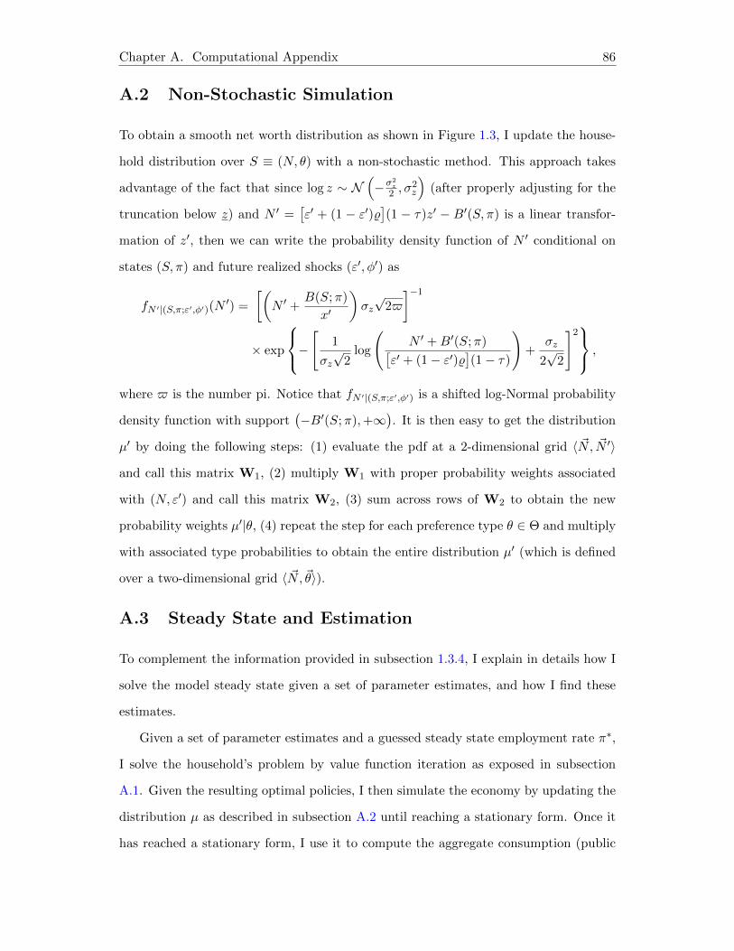
A2 Non-Stochastic Simulation 86
A3 Steady State and Estimation 86
A4 Approximate-Aggregation Equilibrium 87
Chapter 1
The Macroeconomics ofConsumer Finance
11 Introduction
The Financial Crisis of 2007-09 sparked a large body of empirical research emphasizing
a strong and significant relationship between household financial conditions consump-
tion and unemployment (eg Mian and Sufi (2014a) Mian et al (2013) Melzer (2013)
Dynan (2012) Bauer and Nash (2012) Haltenhof et al (2014)) At the trough of the
recession in 2009 more than a million American households filed for bankruptcy while
banks were charging off billions of dollars of consumer loans The tumult was particu-
larly acute in unsecured consumer credit markets where banks halved their originations
of credit card loans representing a fall of more than 50 billion dollars1 In the meantime
the unemployment rate more than doubled in less than two years and households cut
back on their consumption by hundreds of billions of dollars Despite the empirical evi-
dence of a correlation between household finance and business cycle fluctuations there
has been limited progress in the theoretical and quantitative field toward understanding
the key causal mechanism at play2
1Data on bankcard originations is from Experian other data are from US Courts BLS BEA andBoard of Governors
2For instance Justiniano et al (2015) explains that ldquothe macroeconomic consequences of leveragingand deleveraging are relatively minorrdquo while Nakajima and Rıos-Rull (2014) studies models with variousdegrees of credit frictions to conclude that ldquothe volatility of output is highly similar across all economiesrdquoIn opposite in an influential empirical work Mian and Sufi (2014b) use their geographic estimates basedon the non-tradable goods sector to extrapolate that ldquoa 95 reduction in housing net worth (which iswhat the economy experienced between 2007 and 2009) leads to a reduction in overall employment of29 or 55 of the actual decline in total employment of 53rdquo
1
Chapter 1 The Macroeconomics of Consumer Finance 2
The main contribution of this paper is to explain how disturbances in consumer
finance can cause business cycle fluctuations through the rich interplay between credit
and labor risks and to quantify such effects in the US economy As unemployment
rises households are more likely to default translating into tighter credit conditions in
the form of higher interest rates and lower credit limits Such tightening forces indebted
households to decrease consumption which reduces the firmsrsquo sales and thus causes
further unemployment The effects of this consumer credit channel are not limited to
borrowers however Because of higher unemployment unconstrained households also
hold back on consumption to build up precautionary savings Despite its simplicity this
theory is surprisingly powerful in explaining the high volatility and high first-order auto-
correlation of US unemployment as well as key properties of unsecured credit markets
the weak correlation between bankruptcies and unemployment the large volatility of
bankruptcies and the pro-cyclicality of revolving credit My results highlight the role
of consumer credit frictions (incomplete markets intermediation risk of default) in
shaping the cyclical dynamics of employment and consumption
The results are based on a standard dynamic stochastic general equilibrium model
where production is based on labor markets are incomplete and households can hold
unsecured credit accounts Households face two types of idiosyncratic shocks labor
productivity and employment status They can also differ in their preferences which
remain fixed throughout time There are risk-neutral intermediaries who are perfectly
competitive and price individual credit loans according to the householdrsquos specific risk
of default The key novelty of this framework is the treatment of unemployment In
a typical bond economy the funds market clears through the adjustment of a single
interest rate on lending and borrowing and so the goods market clears by Walrasrsquo
law3 However in my model because of the presence of financial intermediaries this
adjustment process becomes inoperative Instead excesses and shortages of goods are
eliminated by adjustments in the firmrsquos production process through its choice of labor
For illustrative purposes consider the following two polar cases On one hand if the
3Walrasrsquo law states that in general equilibrium clearing all but one market ensures equilibrium inthe remaining market
Chapter 1 The Macroeconomics of Consumer Finance 3
unemployment rate were extremely high in the economy production (quantity supplied)
would be low because few households work but consumption (quantity demanded)
would be high because households would tend to dis-save or consume on credit to
compensate for their unemployment spell On the other hand if unemployment were
extremely low production would be high but consumption would not necessarily be as
high because some households would be saving their income for precautionary reasons
Overall the model admits an interior solution where the number of workers employed
by the firms is consistent with the level of production required to satisfy all the goods
demanded by the households Therefore my paper provides a Neoclassical theory of
unemployment purely based on consumer credit frictions rather than traditional frictions
like search or price stickiness
To discipline the quantitative analysis I use the triennial Survey of Consumer Fi-
nance over the sample period 1995-2013 to estimate the model parameters by matching
a large set of aggregate and cross-sectional steady-state moments related to unsecured
consumer credit markets and employment At the aggregate level the model reproduces
well the unemployment rate the credit card interest spread (average credit card inter-
est rate minus fed fund rate) the bankruptcy rate (number of non-business bankruptcy
filings under Chapter 7 as a fraction of civilian population) the total outstanding re-
volving credit expressed as a fraction of aggregate disposable income and to some extent
the charge-off rate on credit cards At the cross-sectional level the model matches the
cross-sectional mean and higher order moments (variance skewness kurtosis) of the dis-
tribution of balance-to-income ratios (a measure of leverage in unsecured credit markets)
and the distribution of credit card interest rates for non-convenience users (ie credit
card users who do not fully repay their balance within a billing cycle) The model also
reproduces the apparent disconnect between credit card interest rates and unsecured
leverage observed in the data (cross-sectional correlation close to zero) The model is
able to replicate all these aggregate and cross-sectional features because it allows for
heterogeneity among households in their income shocks subjective discount factors and
elasticities of intertemporal substitution In a counterfactual estimation with only in-
Chapter 1 The Macroeconomics of Consumer Finance 4
come heterogeneity I show the cross-sectional dispersion in unsecured leverage is almost
three times lower than the data and leverage is almost perfectly correlated with the
interest rate This stems from the fact that with only one dimension of heterogeneity
interest rates are directly a function of leverage Therefore as leverage rises the cost of
borrowing necessarily increases as well which discourages households to lever up and
yields a limited dispersion in leverage
Turning to business cycle analysis I solve the model by conjecturing an approximate-
aggregation equilibrium where individuals only use information about current employ-
ment to form an expectation about future employment conditional on the realization of
future shocks rather than using the entire household distribution as a state variable 4
In my model business cycles are driven by exogenous shocks that affect the way inter-
mediaries discount time More precisely intermediaries are modeled as more impatient
when they lend money to the households compared to when they borrow from them (ie
when they hold deposits) During bad times the spread between these two subjective
discount factors increases Such time-varying spread captures all the different possi-
ble factors that could affect the intermediariesrsquo lending decision (eg time-varying risk
aversion cost of processing loans illiquidity of funds market etc) I infer the volatility
and persistence of this financial shock by parameterizing the model such that it repro-
duces the persistence and volatility of credit card interest rate spread observed in US
data (defined as average credit card interest rate minus effective Fed funds rate) Under
this parametrization I show that the model matches well the unemployment dynamics
as well as salient features of consumer finance In what follows I summarize the key
predictions of the model
First unemployment is highly volatile and highly persistent both in the model and
in the data The volatility of unemployment represents a quarter of its mean and the
coefficient of auto-correlation is close to unity In the model it takes more than ten
years for the economy to recover from a one-quarter recession Similarly credit card
interest spread is highly volatile and persistent and displays a high positive correlation
4See Krusell and Smith (1998) The method I use to solve the model is of independent interest andexplained in details in the computational appendix
Chapter 1 The Macroeconomics of Consumer Finance 5
with unemployment
Second bankruptcies and unemployment are weakly correlated At first glance this
seems to suggest that consumer default does not affect the business cycle However
this is not the case due to the subtle distinction between expected default and realized
default Realized default does not play a significant role because bankruptcies are
extremely rare (less than half a percent of the population per year in model and data)
On the other hand expected default is strongly counter-cyclical (proxied by credit
spreads) and can have large macroeconomic effects because it affects all the borrowers
through high interest rates and low credit limits
Third credit is pro-cyclical This means that households borrow more during an
expansion rather than during a recession This result is counter-intuitive to most
intertemporal-consumption-choice models which predict that households save during
expansions and borrow during recessions in order to smooth their consumption path
This argument however misses a selection effect When unemployment is low house-
holds are less likely to default and thus benefit from higher credit limit and lower interest
rates During an expansion there are more consumers that have access to credit mar-
kets which leads to higher levels of debt overall although each household does not
necessarily borrow more individually
Fourth in the model-based cross section the biggest drop in consumption comes
from the low-net-worth (high debt low income) households who are no longer able to
consume on credit as they did before the crisis In particular the average drop in
consumption at the first quintile of the household distribution is twice as large as in
the second and third quintiles and three times larger than the fourth and fifth quintile
Such disparities across consumption groups also justifies the need to match the right
amount of heterogeneity observed in the data
Fifth in the model even the wealthiest households increase their savings and re-
duce their consumption during a recession This result is due to an aggregation effect
Although it is true that the wealthy households who become unemployed dis-save in
order to smooth consumption it turns out that the ones who remain employed also save
Chapter 1 The Macroeconomics of Consumer Finance 6
more against the higher chances of being unemployed Overall the latter group is dom-
inant and therefore aggregate savings increase among the wealthiest while consumption
decreases
The rich interplay between labor risk credit risk and the aggregate demand channel
offers some new perspectives on public policies Through the lens of the model we can
view consumption and unemployment fluctuations as a symptom of time-varying risk-
sharing opportunities Hence to stimulate the economy we could design policies aimed
at reducing the idiosyncratic risk faced by households rather than simply spending more
Such policies could for example feature a household bailout or some other credit market
regulations Of course the cost and benefit of each policy should be carefully analyzed
in a structurally estimated model This paper makes some progress toward this goal
The remainder of the paper is organized as follows After describing how my paper
fits in the literature I start Section 12 with a description of the model and then
estimate its parameters in steady state in Section 13 Section 14 presents and discusses
the main business cycle results of the paper Section 15 concludes with some remarks
111 Literature
This paper belongs to the vast literature on incomplete-market economies (eg Bewley
(1983) Imrohoroglu (1989) Huggett (1993) Aiyagari (1994) Krusell and Smith (1998)
Wang (2003) Wang (2007) Challe and Ragot (2015)) with an emphasis on consumer
credit default as in Chatterjee et al (2007) Livshits et al (2007) Athreya et al (2009)
and Gordon (2014) In a closely related paper Nakajima and Rıos-Rull (2014) extends
Chatterjee et al (2007) to a dynamic setup to study the business cycle implications of
consumer bankruptcy The main difference with my paper is that the authors do not
consider the interplay between credit risk and labor risk (in their model there is a labor-
leisure trade off but no unemployment) As a result they find that ldquothe volatility of
output is highly similar across all economies [with different degrees of credit frictions]rdquo
My work contributes to the growing body of research that studies the macroeconomic
effects of household financial conditions With the exception of few papers like Nakajima
Chapter 1 The Macroeconomics of Consumer Finance 7
and Rıos-Rull (2014) it has been standard in this literature to drop either of the two
main assumptions that my paper emphasizes (i) aggregate uncertainty (ii) incomplete
markets
Prominent papers of the former group are Eggertsson and Krugman (2012) Guer-
rieri and Lorenzoni (2011) and Justiniano et al (2015) Such models prevent a formal
business cycle analysis since they miss the effects of aggregate risk on householdsrsquo bor-
rowing saving and defaulting decisions which are crucial in order to understand the
aggregate effects of consumer finance on consumption and unemployment
Important papers of the latter group are Herkenhoff (2013) Bethune (2014) Midri-
gan and Philippon (2011) and Kehoe et al (2014) Such papers abstract from market
incompleteness to focus on the role of various financial frictions like price stickiness and
cash-in-advance constraints or credit and labor search
My work also complements the literature which focuses on the firm side (eg Kiy-
otaki and Moore (1997) Bernanke et al (1999) Jermann and Quadrini (2012) Brunner-
meier and Sannikov (2014) Gomes and Schmid (2010a) and Shourideh and Zetlin-Jones
(2014)) Although there could be some overlaps between the two strands of literature
there are virtues in studying each side For instance when firms face credit frictions
that impede their ability to invest or produce they are eventually forced to exit or lose
market shares to the benefit of bigger firms that do not face such frictions In opposite
if households face credit frictions that hinder their ability to consume they will nei-
ther ldquoexitrdquo the economy nor ldquolose market sharesrdquo to wealthier households The lack of
consumption from credit-constrained households is not necessarily offset by more con-
sumption from unconstrained households as I show in my paper thus having aggregate
consequences on consumption and unemployment
12 Modeling Consumer Finance and Systemic Risk
This section describes a parsimonious incomplete-market heterogeneous-agent bond
economy in which households have the option to default Production is stochastic
and based on labor Wages are set in perfectly competitive labor markets and reflect
Chapter 1 The Macroeconomics of Consumer Finance 8
household-specific labor productivities The interest rate on saving and the cross sec-
tion of household-specific interest rates on borrowing are set by perfectly competitive
risk-neutral intermediaries who make zero profit in expectation Since interest rates
are pinned down by intermediaries there is only one variable left to clear the goods
market employment Except for market incompleteness and financial intermediation
the model is a standard Neoclassical framework prices are perfectly flexible goods and
labor markets are frictionless and firms are perfectly competitive
121 The Environment
The economy is populated by a unit continuum of infinitely lived households indexed by
i Time is discrete indexed by t and goes forever Households discount time at their
own subjective rate βi isin (0 1) and order stochastic streams of consumption goods
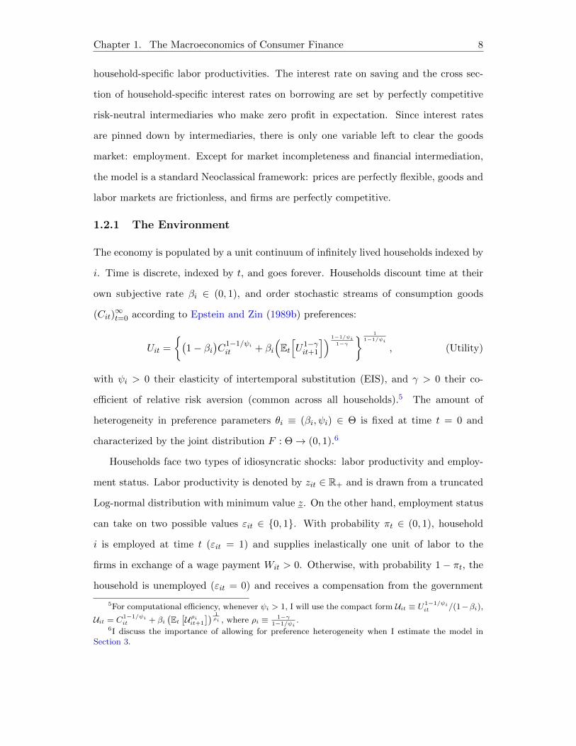
(Cit)infint=0 according to Epstein and Zin (1989b) preferences
Uit =
(1minus βi
)C
1minus1ψiit + βi
(Et[U1minusγit+1
]) 1minus1ψi1minusγ
1
1minus1ψi
(Utility)
with ψi gt 0 their elasticity of intertemporal substitution (EIS) and γ gt 0 their co-
efficient of relative risk aversion (common across all households)5 The amount of
heterogeneity in preference parameters θi equiv (βi ψi) isin Θ is fixed at time t = 0 and
characterized by the joint distribution F Θrarr (0 1)6
Households face two types of idiosyncratic shocks labor productivity and employ-
ment status Labor productivity is denoted by zit isin R+ and is drawn from a truncated
Log-normal distribution with minimum value z On the other hand employment status
can take on two possible values εit isin 0 1 With probability πt isin (0 1) household
i is employed at time t (εit = 1) and supplies inelastically one unit of labor to the
firms in exchange of a wage payment Wit gt 0 Otherwise with probability 1 minus πt the
household is unemployed (εit = 0) and receives a compensation from the government
5For computational efficiency whenever ψi gt 1 I will use the compact form Uit equiv U1minus1ψiit (1minusβi)
Uit = C1minus1ψiit + βi
(Et[Uρiit+1
]) 1ρi where ρi equiv 1minusγ
1minus1ψi
6I discuss the importance of allowing for preference heterogeneity when I estimate the model inSection 3
Chapter 1 The Macroeconomics of Consumer Finance 9
at the replacement rate isin (0 1)7 The unemployment insurance program is funded
by a proportional tax τ isin (0 1) on income and any fiscal surplus is spent as public
consumption Gt Labor income net of taxes equals
Υit = (1minus τ)(εit + (1minus εit)
)Wit (Income)
The key feature of this model is that the employment probability πt isin (0 1) is simply
pinned down by the firms A representative firm operates the economy by choosing
labor πt isin (0 1) and producing a single non-durable good Yt isin R+ with the linear
technology
Yt =
intεitzit di hArr Yt = πt (Technology)
where the equivalence result holds because of the assumption that employment shocks
εit are iid across households and the mean of the idiosyncratic productivity draws
zit is normalized to unity Under competitive pricing workers are paid their marginal
product hence Wit = zit
Markets are incomplete in the sense that households are not allowed to trade con-
sumption claims contingent on their idiosyncratic shocks (εit zit) This could be due to
a moral hazard problem though it is not explicitly modeled in this paper Households
only have access to a credit account with balance Bit isin R where Bit le 0 is treated as
savings with return rft gt 0 The price of $1 borrowed today by household i is denoted
by qit le 1 and reflects her specific risk of default At any point in time household i is
free to default on her credit balance Bit gt 0 By doing so her outstanding debt is fully
discharged (Bit equiv 0) Consequently the household is not allowed to save or borrow
in the current period (one-period autarky) and Υit minusΥ dollars are garnished from her
income where Υ is an exogenous limit on the amount of income the intermediaries can
seize8
7Notice that the modeling of the US unemployment insurance is simplified along two dimensionsto reduce the state space First benefits are computed in terms of the wage the household would haveearned if employed which corresponds to the wage of an actual employed worker who has the exactsame productivity In opposite the US benefits are computed with respect to the wage earned beforethe job was lost hence requiring an extra state variable Second benefits are perpetual Instead in theUS they are limited to a certain number of periods which would have to be tracked by an additionalstate variable
8This specification of wage garnishment allows me to express the householdrsquos recursive problem
Chapter 1 The Macroeconomics of Consumer Finance 10
There exists a large number of risk-neutral intermediaries with identical prefer-
ences They discount time differently whether they lend resources to households or
borrow from them (ie hold saving account) In particular they use the discount factor
δ isin (0 1) when making a borrowing decision and φtδ otherwise when lending money to
households The spread between the two discount factors is the sole source of business
cycle fluctuations and is modeled as a first-order Markov chain φt isin φ1 φN with
transition probabilities Pr(φt+1 = φj |φt = φi) equiv πij such thatsumN
j=1 πij = 1 for all
i = 1 N This financial shock captures different factors that could affect the inter-
mediariesrsquo lending decisions such as time-varying risk aversion funds market illiquidity
costly processing loans etc
122 Householdrsquos Problem
At the beginning of each period t household i observes her idiosyncratic shocks (εit zit) isin
R2+ her outstanding balance Bit isin R as well as the aggregate state of the economy
ωt isin Ωt (discussed below) and decides whether to default on her debt if any
Vit = maxV defit V pay
it
(11)
The value of paying off her debt is
V payit = max
Bit+1leB
C
1minus1ψiit + βi
(Et[V 1minusγit+1
]) 1minus1ψi1minusγ
1
1minus1ψi
subject to
Υit + qitBit+1 ge Cit +Bit (Budget constraint)
(12)
where B isin R+ is an exogenous limit that prevents her from running Ponzi schemes9 As
the household i is more likely to default she faces a higher cost of rolling over her debt
and therefore qit decreases Notice that in the limiting case that household i will almost
surely default next period her cost of borrowing becomes infinite In that case the
household cannot borrow since qit rarr 0 and thus qitBit+1 rarr 0 regardless of the choice
solely in terms of her net worth Nit equiv Υit minus Bit which greatly simplifies the computational methodFor technical reasons I restrict Υ le (1 minus τ)z to ensure that Υit minus Υt ge 0 at any point in time (ieextremely poor households do not get a subsidy from the banks by defaulting on their debt)
9In practice B represents the upper limit of the grid for the state Bit and is set to a value largeenough so that the householdrsquos optimal choice of debt does not bind
Chapter 1 The Macroeconomics of Consumer Finance 11
Bit+1 le B Upon default household i contemplates one-period autarky her debt is
discharged her income is garnished by the amount Υit minusΥ and she cannot borrow or
save at time t Mathematically
V defit =
C
1minus1ψiit + βi
(Et[V 1minusγit+1
]) 1minus1ψi1minusγ
1
1minus1ψi
where
Cit equiv Υit Υit equiv Υ Bit equiv 0 Bit+1 equiv 0
(13)
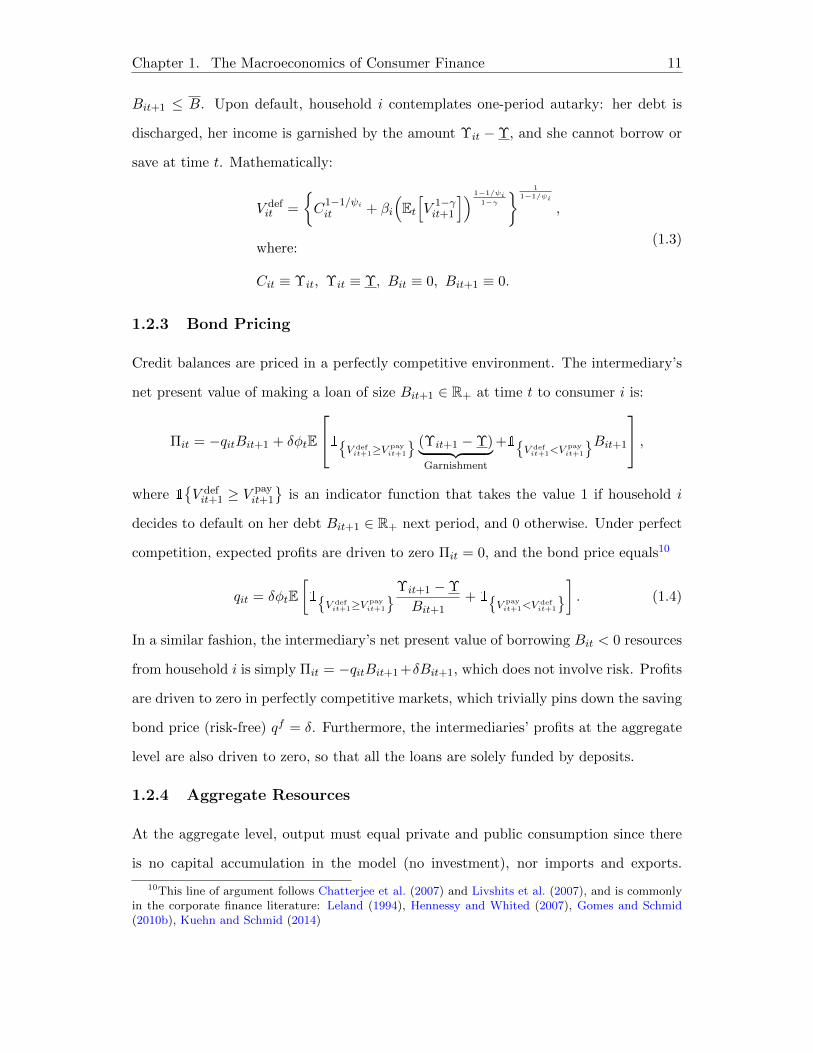
123 Bond Pricing
Credit balances are priced in a perfectly competitive environment The intermediaryrsquos
net present value of making a loan of size Bit+1 isin R+ at time t to consumer i is
Πit = minusqitBit+1 + δφtE
1V defit+1geV
payit+1
(Υit+1 minusΥ)︸ ︷︷ ︸Garnishment
+1V defit+1ltV
payit+1
Bit+1
where 1
V defit+1 ge V
payit+1
is an indicator function that takes the value 1 if household i
decides to default on her debt Bit+1 isin R+ next period and 0 otherwise Under perfect
competition expected profits are driven to zero Πit = 0 and the bond price equals10
qit = δφtE[1
V defit+1geV
payit+1
Υit+1 minusΥ
Bit+1+ 1
V payit+1ltV
defit+1
] (14)
In a similar fashion the intermediaryrsquos net present value of borrowing Bit lt 0 resources
from household i is simply Πit = minusqitBit+1+δBit+1 which does not involve risk Profits
are driven to zero in perfectly competitive markets which trivially pins down the saving
bond price (risk-free) qf = δ Furthermore the intermediariesrsquo profits at the aggregate
level are also driven to zero so that all the loans are solely funded by deposits
124 Aggregate Resources
At the aggregate level output must equal private and public consumption since there
is no capital accumulation in the model (no investment) nor imports and exports
10This line of argument follows Chatterjee et al (2007) and Livshits et al (2007) and is commonlyin the corporate finance literature Leland (1994) Hennessy and Whited (2007) Gomes and Schmid(2010b) Kuehn and Schmid (2014)
Chapter 1 The Macroeconomics of Consumer Finance 12
Furthermore since intermediariesrsquo aggregate profits are driven to zero under pure and
perfect competition their consumption is null Therefore
Yt = Ct +Gt (15)
Private consumption is simply the sum of householdsrsquo individual consumptions Ct =intCit di On the other hand public consumption consists of the government expendi-
tures financed by income taxes and net of transfers
Gt =
intτzitεit di︸ ︷︷ ︸
Fiscal revenue
minusint(1minus τ)zit(1minus εit) di︸ ︷︷ ︸Unemployment transfers
which is simply Gt = τπt minus (1 minus τ)(1 minus πt) since the employment shocks εit isin 0 1
are iid across households and the cross-sectional mean of the idiosyncratic productivity
shocks is normalized to unity For τ isin (0 1) large enough compared to isin (0 1) Gt is
always positive and co-moves with the employment rate (pro-cyclical)
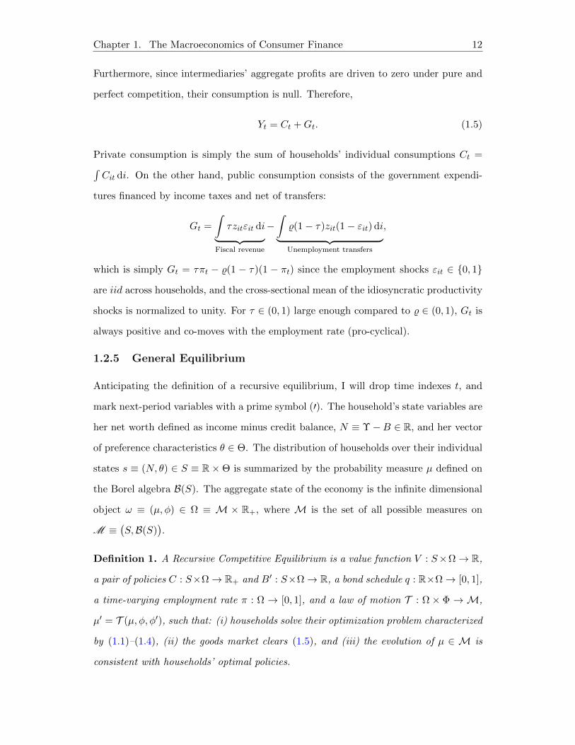
125 General Equilibrium
Anticipating the definition of a recursive equilibrium I will drop time indexes t and
mark next-period variables with a prime symbol (prime) The householdrsquos state variables are
her net worth defined as income minus credit balance N equiv ΥminusB isin R and her vector
of preference characteristics θ isin Θ The distribution of households over their individual
states s equiv (N θ) isin S equiv RtimesΘ is summarized by the probability measure micro defined on
the Borel algebra B(S) The aggregate state of the economy is the infinite dimensional
object ω equiv (micro φ) isin Ω equiv M times R+ where M is the set of all possible measures on
M equiv(SB(S)
)
Definition 1 A Recursive Competitive Equilibrium is a value function V StimesΩrarr R
a pair of policies C StimesΩrarr R+ and Bprime StimesΩrarr R a bond schedule q RtimesΩrarr [0 1]
a time-varying employment rate π Ω rarr [0 1] and a law of motion T Ω times Φ rarrM
microprime = T (micro φ φprime) such that (i) households solve their optimization problem characterized
by (11)ndash(14) (ii) the goods market clears (15) and (iii) the evolution of micro isin M is
consistent with householdsrsquo optimal policies
Chapter 1 The Macroeconomics of Consumer Finance 13
Notice that if markets were complete and preferences identical every household
would consume the average private income of the economy Et[Υit] = (1 minus τ)(πt +
(1 minus πt)) Consequently the goods market would clear regardless of the employment
rate11 In particular full employment is one of the equilibria in the complete-market
case Hence the level of unemployment in the full model is an implicit measure of the
degree of market incompleteness faced by consumers
126 Steady State
It will be useful to define the model (non-stochastic) steady state as follows12
Definition 2 A Steady State Equilibrium is a value function v(sπlowast) a pair of policies
c(sπlowast) and bprime(sπlowast) a bond schedule q(bprimeπlowast) a constant employment rate πlowast isin [0 1]
and a time-invariant distribution microlowast isinM such that (i) households solve their dynamic
program problem stated in (11)ndash(14) but without aggregate uncertainty (ii) the goods
market clears (15) and (iii) microlowast = T (microlowast) where T corresponds to the operator T in an
environment without aggregate risk
In absence of aggregate uncertainty the distribution microlowast is time-invariant and hence
not part of the household state space Instead I wrote the householdrsquos value and policies
as explicit functions of πlowast to highlight the fact that the employment rate is the only
aggregate variable that the household cares about This is an insight that will prove
useful in the following section where I describe the solution method
127 Solution Method
Since there are no known closed-form solution for this class of model I will rely on
numerical methods to solve the model This task is however computationally challenging
since the state micro is an infinite dimensional object Following Krusell and Smith (1998)
I will remedy to this problem by conjecturing that the equilibrium features approximate
aggregation in the sense that the entire households distribution can be summarized by
11To see this πt︸︷︷︸GDP
= (1minus τ)(πt + (1minus πt)
)︸ ︷︷ ︸Consumption
+ τπt minus (1minus τ)(1minus πt)︸ ︷︷ ︸Government expenditure
rArr πt = πt
12Technically an equilibrium with idiosyncratic shocks (ε z) but no aggregate (financial) shocks (φ)
Chapter 1 The Macroeconomics of Consumer Finance 14
a finite set of moments In their seminal paper the authors used statistical moments
of the idiosyncratic state variable (eg mean variance) to proxy for the distribution
Subsequent research has explored the use of alternative moments such as prices (eg
interest rate in Krusell and Smith (1997))
Observe that in my model in order to solve their optimization problem defined by
(11)ndash(14) households only need to forecast the next-period employment rate πprime in
order to form expectations Implicitly this means that they do not require any specific
information about the distribution micro isinM itself but rather need some good predictors
of πprime I conjecture and verify that current employment π is a good predictor of next-
quarter employment πprime conditional on the realization of future shocks φprime Formally I
define
Definition 3 An Approximate-Aggregation Equilibrium is a value function V S times
(0 1) rarr R a pair of policies C S times (0 1) rarr R+ and Bprime S times (0 1) rarr R a bond
schedule q R times (0 1) rarr [0 1] and a forecasting rule πprime = Γ(π φprime) + ε such that (i)
households solve their optimization problem characterized by (11)ndash(14) (ii) the goods
market clears (15) and (iii) the forecasting errors ε isin E are near zero
13 Estimating the Model Steady State
The first test of the model is whether it can explain the unemployment rate and a
large set of aggregate and cross-sectional consumer finance statistics in the steady state
under plausible parameter values I discipline this exercise in an over-identified moment
matching procedure Except for few parameters that have a clear counterpart in the
data (eg income tax rate and unemployment insurance replacement rate) all the other
model parameters are estimated by minimizing the squared relative distance between
simulated and actual moments The main result of this section is that under a plausible
parametrization the model can replicate the steady state unemployment rate while
matching simultaneously a high credit card spread a low bankruptcy rate and a large
cross-sectional dispersion in both unsecured leverage and credit card interest rates
Chapter 1 The Macroeconomics of Consumer Finance 15
131 The Data
The main data that I use to estimate the model is the Survey of Consumer Finances
(SCF) from the Board of Governors All the cross sectional moments are averaged
across the seven triennial surveys available over the period 1995ndash2013 To assess the
amount of heterogeneity in cost of borrowing and amounts borrowed in the unsecured
credit markets I look at two key variables the balance-to-income ratio and the credit
card interest rate The first variable that I consider is the balance-to-income ratio
which proxies for leverage in absence of collaterals The balance refers to the amount
of money the household still owes to the bank after her last payment This means
that the balance after payment excludes the typical ldquoconveniencerdquo credit that does not
entail interest fees if paid in full within a billing cycle On the other hand the income
refers to the annual gross income before taxes This includes all wages and salaries
unemployment compensations pensions and other social security transfers and income
from interests capital gains and business ownership The second variable I consider is
the interest rate paid on the most used credit card This is a variable that started to
be documented only in 1995 (except for the 1983 survey) The cross section of interest
rates only reflects credit card holders who are revolvers and not simply convenience
users
I complement the SCF data with various aggregate statistics such as the credit
card interest rate spread the bankruptcy rate the credit card charge-off rate and the
ratio of revolving credit to aggregate disposable income I construct the credit card
spread by taking the difference between the average credit card interest rate and the
effective Federal Funds rate The former is reported in H15 Selected Interest Rates
(Board of Governors) while the latter is documented in the Report on the Profitability
of Credit Card Operations (Board of Governors) On the other hand the bankruptcy
rate is obtained by dividing non-business bankruptcy filings under Chapter 7 (US
Bankruptcy Courts) by the US population (civilian non-institutional of age 16 and
older)13 To compute the ratio of outstanding revolving credit to disposable income
13Consumers can file for bankruptcy under three different chapters 7 11 and 13 Chapter 11 relates
Chapter 1 The Macroeconomics of Consumer Finance 16
I use the data on total outstanding revolving consumer credit from G19 Consumer
Credit (Board of Governors) and the aggregate disposable personal income reported in
Personal Income and Outlays A067RC1 (Bureau of Economic Analysis) The charge-off
rate is documented in the Report of Condition and Income (Board of Governors)The
charge-offs are the loans that are removed from the banksrsquo books and charged as a loss
The charge-off rate is net of recoveries and computed as the ratio between charge-offs
and the banksrsquo outstanding debt Lastly the civilian unemployment rate is from the
US Bureau of Labor Statistics (BLS)
132 Mapping the Model to US Data
A difficulty in mapping the model to the data is to distinguish between the credit card
holders who carry a balance from one period to another (revolvers) and the ones who pay
their balance in full within a billing cycle (convenience users) This stems from the fact
that in the model there is no distinction between cash and debt Thus the householdrsquos
explicit decision to pay-off a portion of her outstanding debt with cash instead of issuing
new debt is indeterminate14 To tackle this issue I split the consumers in my model
as follows Convenience users refer to the consumers who do not roll over their debt
that is if there were a cash flow mismatch within a period t they would be able to pay
off their existing debt with their current income alone Instead the revolvers will refer
to the consumers who need to borrow in order to pay off their past debt In terms of
state variables this means that the revolvers are the households whose current income
is smaller than current debt Υ lt B which implies that they have a negative net worth
N lt 0 On the other hand the convenience users are the ones who have enough income
to cover their debt Υ ge B or simply N ge 0
to business owners and concerns less than 1 of all the filings On the other hand Chapter 11 represents30 of all the filings but involves a repayment plan which is something that my model does not accountfor As a consequence I only consider the filings under Chapter 7 (over 69 of the bankruptcy cases)There is a spike in bankruptcy filings around 2005 which reflects the Bankruptcy Abuse and Preventionand Consumer Protection Act (BAPCPA) that took effect on October 17 2005
14Mathematically let Xit be cash and Lit the size of a new credit card loan then the credit balancersquoslaw of motion is
Bit+1 = Bit minusXit + Lit
In the model only Bit+1 and Bit are separately identified but not Xit and Lit
Chapter 1 The Macroeconomics of Consumer Finance 17
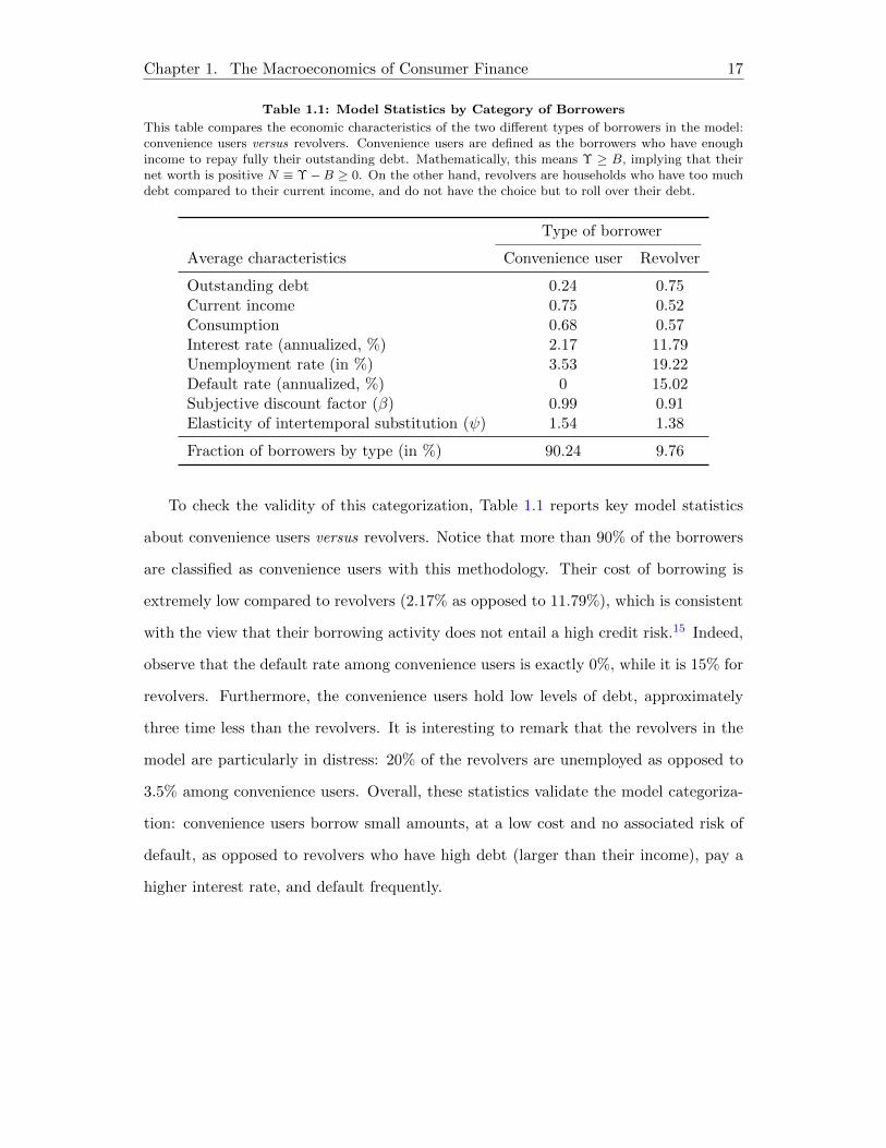
Table 11 Model Statistics by Category of Borrowers
This table compares the economic characteristics of the two different types of borrowers in the modelconvenience users versus revolvers Convenience users are defined as the borrowers who have enoughincome to repay fully their outstanding debt Mathematically this means Υ ge B implying that theirnet worth is positive N equiv ΥminusB ge 0 On the other hand revolvers are households who have too muchdebt compared to their current income and do not have the choice but to roll over their debt
Type of borrower
Average characteristics Convenience user Revolver
Outstanding debt 024 075Current income 075 052Consumption 068 057Interest rate (annualized ) 217 1179Unemployment rate (in ) 353 1922Default rate (annualized ) 0 1502Subjective discount factor (β) 099 091Elasticity of intertemporal substitution (ψ) 154 138
Fraction of borrowers by type (in ) 9024 976
To check the validity of this categorization Table 11 reports key model statistics
about convenience users versus revolvers Notice that more than 90 of the borrowers
are classified as convenience users with this methodology Their cost of borrowing is
extremely low compared to revolvers (217 as opposed to 1179) which is consistent
with the view that their borrowing activity does not entail a high credit risk15 Indeed
observe that the default rate among convenience users is exactly 0 while it is 15 for
revolvers Furthermore the convenience users hold low levels of debt approximately
three time less than the revolvers It is interesting to remark that the revolvers in the
model are particularly in distress 20 of the revolvers are unemployed as opposed to
35 among convenience users Overall these statistics validate the model categoriza-
tion convenience users borrow small amounts at a low cost and no associated risk of
default as opposed to revolvers who have high debt (larger than their income) pay a
higher interest rate and default frequently
Chapter 1 The Macroeconomics of Consumer Finance 18
-2 0 2 40
05
1
15
2
25
Net worth
Con
sum
ptio
n
0 1 2 302
04
06
08
1
Loan size
Bon
d sc
hedu
le
-2 0 2 4
-3
-2
-1
0
1
2
3
Net worth
Nex
t-pe
riod
cre
dit b
alan
ce
-2 0 2 40
10
20
30
Net worth
Ann
ual i
nter
est r
ate
NormalLow ψLow β
NormalLow ψLow β
Figure 11 Steady-State Policy Functions by Household TypeThis figure depicts the householdsrsquo optimal consumption policy their optimal next-period choice ofcredit balance (negative balances are savings) the optimal bond schedule offered by the intermediaries(given householdsrsquo optimal behavior) and the equilibrium interest rate for each type of households(evaluating the bond schedule at the householdsrsquo optimal borrowing policies) There are three typesnormal impatient (low β) and high-incentive to smooth consumption (low ψ low EIS) Notice thatthe default cutoffs are near zero for the normal households and the impatient ones and near minus2 for thelow-EIS households
133 Identifying Preference Heterogeneity in the Data
To estimate the amount of preference heterogeneity required to match the large disper-
sion of balance-to-income ratios and credit card interest rates I consider three different
types of households in my model high medium and low High-type households are
highly levered but their cost of borrowing is low Low-type households are also highly
levered and their cost of borrowing is high Finally medium-type households have low
leverage and with moderate cost of borrowing I identify these three types in the model
15In the model the cost of borrowing for the convenience users is not exactly zero because theystill need to compensate the intermediaries for their impatience In reality the convenience users donot have to pay an interest fee because banks get paid fees by the merchants who use credit card as amethod of payment
Chapter 1 The Macroeconomics of Consumer Finance 19
by looking at the household optimal policies in steady state (see Figure 11)
In particular high-type households have a relatively low elasticity of intertemporal
substitution (ψ) compared to the other types and low-type households have a rela-
tively low subjective discount factor (β) Notice in particular how households with low
patience tend to borrow more while paying high interest rates In the meantime house-
holds with a low EIS are able to borrow more at lower net worth levels for a low cost
This stems from the fact that with a low elasticity of intertemporal substitution (EIS)
such households have a strong desire to smooth consumption and thus they want to
avoid a default event Since household types are observable16 the intermediaries rec-
ognize that such households have strong incentives not to default and hence they offer
them a discount For computational tractability I consider the following distribution
of types (β ψ) (β ψ) (β ψ) which requires the estimation of only four parameters
(high and low value for β and ψ respectively) and two associated probabilities (the
third probability being linearly dependent)
134 Matching Moments
I proceed in two stages to estimate the values of the different parameters of the model
In the first stage I directly assign values to the parameters that have a clear counterpart
in the data Three parameters are calibrated in this fashion the income tax rate τ the
Unemployment Insurance (UI) replacement rate and the risk-free return on saving
account rf (which I interpret in the data as the effective Federal Funds rate) In the
second stage I obtain the rest of the parameter values (six out of nine) by minimizing
the squared relative difference between a set of actual and simulated moments Six
parameters concern preference heterogeneity Three other parameters are the steady
state value of the financial shock (the intermediariesrsquo discount spread) E[φ] the volatility
of the idiosyncratic labor productivity shock σz and the coefficient of relative risk
aversion γ (common across households)
To identify the parameter values I select several cross-sectional and aggregate mo-
16The assumption that types are observable proxies for the fact that in reality creditors have access tocredit scores which keep track of the householdsrsquo borrowing habits and hence provides useful informationto infer their type
Chapter 1 The Macroeconomics of Consumer Finance 20
ments such as the employment rate the bankruptcy rate the credit card charge-off rate
the ratio of outstanding revolving credit to disposable income the cross-sectional mean
variance skewness and kurtosis of balance-to-income ratios the cross-sectional mean
variance skewness and kurtosis of credit card interest rates the cross-sectional corre-
lation between balance-to-income ratios and credit card interest rates and the average
recovery rate on defaulted loans
In total I use 18 cross-sectional and aggregate moments to compute the method-
of-moment objective function which maps a set of 9 parameter estimates to the sum
of squared differences (percentage deviations) between actual and simulated moments
Each function evaluation requires solving the model steady state In particular given a
set of parameters and a guessed steady state employment rate πlowast I solve the householdrsquos
optimization problem and then use her optimal policies to simulate the economy until
the household net worth distribution becomes stationary Given this distribution I then
compute the steady-state aggregate consumption (public and private) Clowast(πlowast) +Glowast(πlowast)
and compare it with aggregate production Y lowast equiv πlowast If they differ I re-start the process
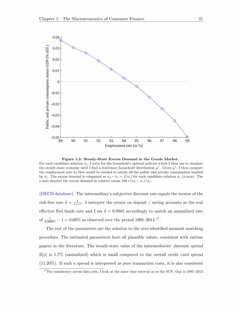
with a new guess for πlowast The steady-state equilibrium can be viewed as the solution to
the fixed point problem Clowast(πlowast) + Glowast(πlowast) minus πlowast = 0 (an excess demand function set to
zero) which I find with a simple bisection method Figure 12 plots such function The
method-of-moment algorithm search for different sets of parameters in parallel with a
genetic algorithm and each set of parameters requires multiple rounds of value function
iterations and non-stochastic simulations to find an associated steady-state equilibrium
135 Results
Table 12 presents the estimated parameter values
The first group of parameters 〈 τ δ〉 have direct counterparts in the data and thus
set accordingly In particular the replacement ratio is set to = 40 in accordance with
the UI Replacement Rates Report (US Department of Labor) The proportional tax rate
on output corresponds to the tax revenue of the government (at all levels) expressed as a
percentage of GDP which is approximately τ = 25 according to the Revenue Statistics
Chapter 1 The Macroeconomics of Consumer Finance 21
89 90 91 92 93 94 95 96 97 98 99-005
-004
-003
-002
-001
0
001
002
003
004
Employment rate (in )
Publ
ic a
nd p
riva
te c
onsu
mpt
ion
min
us G
DP
( d
iff
)
Figure 12 Steady-State Excess Demand in the Goods MarketFor each candidate solution πs I solve for the householdrsquos optimal policies which I then use to simulatethe steady-state economy until I find a stationary household distribution microlowast Given microlowast I then computethe employment rate πd that would be needed to satisfy all the public and private consumption impliedby πs The excess demand is computed as πdminusπs = f(πs) for each candidate solution πs (x-axis) They-axis denotes the excess demand in relative terms 100 lowast (πd minus πs)πs
(OECD database) The intermediaryrsquos subjective discount rate equals the inverse of the
risk-free rate δ = 11+rf I interpret the return on deposit saving accounts as the real
effective Fed funds rate and I set δ = 09985 accordingly to match an annualized rate
of 1099854 minus 1 = 060 as observed over the period 1995ndash201317
The rest of the parameters are the solution to the over-identified moment matching
procedure The estimated parameters have all plausible values consistent with various
papers in the literature The steady-state value of the intermediariesrsquo discount spread
E[φ] is 17 (annualized) which is small compared to the overall credit card spread
(1120) If such a spread is interpreted as pure transaction costs it is also consistent
17For consistency across data sets I look at the same time interval as in the SCF that is 1995ndash2013
Chapter 1 The Macroeconomics of Consumer Finance 22
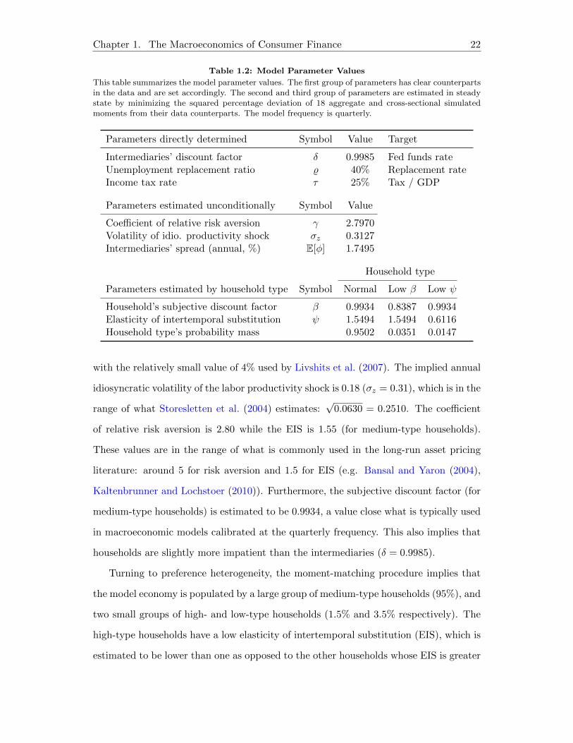
Table 12 Model Parameter Values
This table summarizes the model parameter values The first group of parameters has clear counterpartsin the data and are set accordingly The second and third group of parameters are estimated in steadystate by minimizing the squared percentage deviation of 18 aggregate and cross-sectional simulatedmoments from their data counterparts The model frequency is quarterly
Parameters directly determined Symbol Value Target
Intermediariesrsquo discount factor δ 09985 Fed funds rateUnemployment replacement ratio 40 Replacement rateIncome tax rate τ 25 Tax GDP
Parameters estimated unconditionally Symbol Value
Coefficient of relative risk aversion γ 27970Volatility of idio productivity shock σz 03127Intermediariesrsquo spread (annual ) E[φ] 17495
Household type
Parameters estimated by household type Symbol Normal Low β Low ψ
Householdrsquos subjective discount factor β 09934 08387 09934Elasticity of intertemporal substitution ψ 15494 15494 06116Household typersquos probability mass 09502 00351 00147
with the relatively small value of 4 used by Livshits et al (2007) The implied annual
idiosyncratic volatility of the labor productivity shock is 018 (σz = 031) which is in the
range of what Storesletten et al (2004) estimatesradic
00630 = 02510 The coefficient
of relative risk aversion is 280 while the EIS is 155 (for medium-type households)
These values are in the range of what is commonly used in the long-run asset pricing
literature around 5 for risk aversion and 15 for EIS (eg Bansal and Yaron (2004)
Kaltenbrunner and Lochstoer (2010)) Furthermore the subjective discount factor (for
medium-type households) is estimated to be 09934 a value close what is typically used
in macroeconomic models calibrated at the quarterly frequency This also implies that
households are slightly more impatient than the intermediaries (δ = 09985)
Turning to preference heterogeneity the moment-matching procedure implies that
the model economy is populated by a large group of medium-type households (95) and
two small groups of high- and low-type households (15 and 35 respectively) The
high-type households have a low elasticity of intertemporal substitution (EIS) which is
estimated to be lower than one as opposed to the other households whose EIS is greater
Chapter 1 The Macroeconomics of Consumer Finance 23
than one The low-type households are substantially more impatient than the other
households (08387 compared to 0934)
Table 13 compares the simulated moments with the actual ones observed in the
data
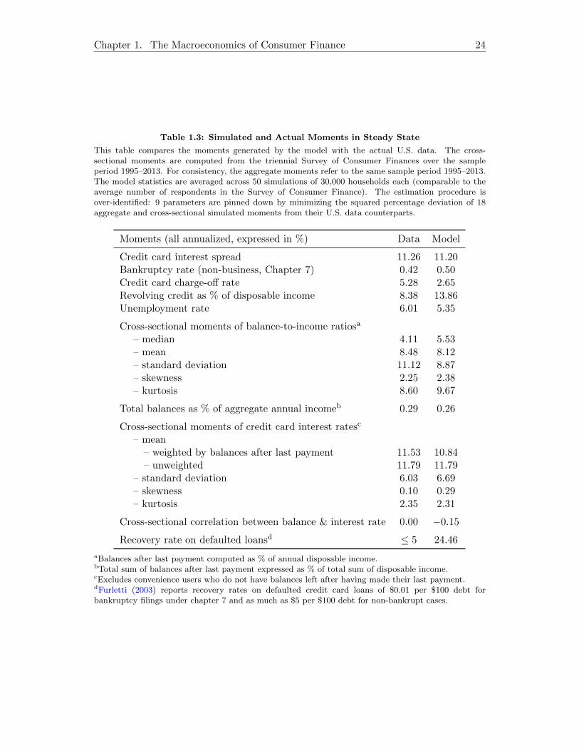
Overall the model does well in replicating the main aggregate and cross-sectional
moments In the cross section of balance-to-income ratios the median is low while
the mean is high both in the model and in the data (411 and 848 compared to 553
and 812) Also all the higher order moments are large in the model and in the data
standard deviation (887 versus 1112) skewness (238 and 225) and kurtosis (967 and
860) The model is also successful in matching the cross-sectional moments of interest
rates a high mean and standard deviation (1179 and 669 compared to 1179 and 603)
and a low skewness and kurtosis close to the Normal law (029 and 231 versus 010 and
235) The model also replicates the apparent disconnect between interest rates and
balance-to-income ratios (cross-sectional correlation of 0 in the data and minus015 in the
model) At the aggregate level the model matches well the credit card interest spread
(1120 in the model and 1126 in the data) the unemployment rate (535 in the model
and 601 in the data) and the bankruptcy rate (050 and 042) but tends to overstate
the ratio of total outstanding revolving credit to aggregate disposable income (1386
compared to 838)
The two main shortcomings of the model relate to the recovery rate on credit card
loans which is too high and the charge-off rate which is too low The model performance
along these dimensions is tied to the garnishment rule since a lower garnishment would
decrease the recovery rate and increase the charge-offs The garnishment rule was
modeled as ΥitminusΥ with the restriction that Υ le (1minus τ)z where z is the lower bound
of the truncated lognormal distribution of idiosyncratic labor productivity shocks Such
assumption made the model tractable by collapsing the householdrsquos state space into net
worth only rather than keeping track of income and debt separately I conjecture that
including z in the set of parameters to be estimated would improve the model fit with
this respect Instead in the current estimation procedure z is arbitrarily fixed at a
Chapter 1 The Macroeconomics of Consumer Finance 24
Table 13 Simulated and Actual Moments in Steady State
This table compares the moments generated by the model with the actual US data The cross-sectional moments are computed from the triennial Survey of Consumer Finances over the sampleperiod 1995ndash2013 For consistency the aggregate moments refer to the same sample period 1995ndash2013The model statistics are averaged across 50 simulations of 30000 households each (comparable to theaverage number of respondents in the Survey of Consumer Finance) The estimation procedure isover-identified 9 parameters are pinned down by minimizing the squared percentage deviation of 18aggregate and cross-sectional simulated moments from their US data counterparts
Moments (all annualized expressed in ) Data Model
Credit card interest spread 1126 1120Bankruptcy rate (non-business Chapter 7) 042 050Credit card charge-off rate 528 265Revolving credit as of disposable income 838 1386Unemployment rate 601 535
Cross-sectional moments of balance-to-income ratiosa
ndash median 411 553ndash mean 848 812ndash standard deviation 1112 887ndash skewness 225 238ndash kurtosis 860 967
Total balances as of aggregate annual incomeb 029 026
Cross-sectional moments of credit card interest ratesc
ndash meanndash weighted by balances after last payment 1153 1084ndash unweighted 1179 1179
ndash standard deviation 603 669ndash skewness 010 029ndash kurtosis 235 231
Cross-sectional correlation between balance amp interest rate 000 minus015
Recovery rate on defaulted loansd le 5 2446
aBalances after last payment computed as of annual disposable incomebTotal sum of balances after last payment expressed as of total sum of disposable incomecExcludes convenience users who do not have balances left after having made their last paymentdFurletti (2003) reports recovery rates on defaulted credit card loans of $001 per $100 debt forbankruptcy filings under chapter 7 and as much as $5 per $100 debt for non-bankrupt cases
Chapter 1 The Macroeconomics of Consumer Finance 25
small value and Υ is set at its maximum possible value
136 Counterfactual Results without Preference Heterogeneity
To check the robustness of all these estimation results I re-estimate the model with
no preference heterogeneity Table 14 presents the estimated parameter values and
the simulated moments obtained from this alternative estimation procedure Notice in
particular that in general all the newly estimated parameters have values comparable
to their benchmark counterparts except for the intermediariesrsquo discount spread that
is considerably understated (17495 in full estimation with preference heterogeneity
compared to 00450 in alternative estimation without preference heterogeneity)
Overall the estimation procedure that does not allow for preference heterogeneity
tends to understate the cross-sectional dispersions in leverage and interest rates It
is particularly true for the former the standard deviation is four times lower in the
alternative estimation compared to the benchmark one and the mean is two times lower
Furthermore not allowing for preference heterogeneity has counter-factual implications
for the relationship between credit card interest rates and balance-to-income ratios
While in the data and in the benchmark case they are weakly correlated (000 and
minus015 respectively) their correlation is strong in the no-preference-heterogeneity case
(096)
137 Understanding the Role of Preference Heterogeneity
A key result of the alternative estimation procedure is that heterogeneity in β and ψ
plays an important role in explaining the large dispersion in balance-to-income ratios
Figure 13 illustrates this point by plotting the household distribution of net worth
balance-to-income ratios and non-convenience interest rates by preference type ldquohighrdquo
(high incentive to smooth low ψ) ldquomediumrdquo (normal) ldquolowrdquo (impatient low β)
What I want to emphasize here is that the β-heterogeneity and the ψ-heterogeneity
have different implications at the cross-sectional level and complement each other in
generating the large dispersion in balance-to-income ratios and credit card interest
rates For instance consider the case of heterogeneity in the elasticity of intertemporal
Chapter 1 The Macroeconomics of Consumer Finance 26
Table 14 Alternative Steady-State Estimation without Preference Heterogeneity
This table compares the moments generated by the model with the actual US data The cross-sectional moments are computed from the triennial Survey of Consumer Finances over the sampleperiod 1995ndash2013 For consistency the aggregate moments refer to the same sample period 1995ndash2013The model statistics are averaged across 50 simulations of 30000 households each (comparable to theaverage number of respondents in the Survey of Consumer Finance) The estimation procedure isover-identified 5 parameters are pinned down by minimizing the squared percentage deviation of 17aggregate and cross-sectional simulated moments from their US data counterparts
Estimated parameters Symbol Value
Subjective discount factor β 09892Elasticity of intertemporal substitution (EIS) ψ 14377Coefficient of relative risk aversion γ 35530Volatility of idiosyncratic productivity shock σz 03022Intermediariesrsquo discount spread (annual ) E[φ] 00450
Moments (all annualized expressed in ) Data Model
Credit card interest spread 1126 846Bankruptcy rate (non-business Chapter 7) 042 050Credit card charge-off rate 528 133Revolving credit as of disposable income 838 588Unemployment rate 601 506
Cross section of balance-to-income ratiosa
ndash median 411 327ndash mean 848 410ndash standard deviation 1112 327ndash skewness 225 086ndash kurtosis 860 292
Total balances as of aggregate annual incomeb 029 012
Cross section of credit card interest ratesc
ndash meanndash weighted by balances after last payment 1153 1261ndash unweighted 1179 905
ndash standard deviation 603 459ndash skewness 010 071ndash kurtosis 235 239
Cross-sectional correlation between balance amp interest rate 000 096
aBalances after last payment computed as of annual disposable incomebTotal sum of balances after last payment expressed as of total sum of disposable incomecExcludes convenience users who do not have balances left after having made their last payment
Chapter 1 The Macroeconomics of Consumer Finance 27
substitution ψ By having low-ψ households who dislike default the model generates a
group of ldquoprimerdquo borrowers who can borrow a lot at a discounted interest rate If there
were only one dimension of heterogeneity interest rates would be directly a function
of leverage and therefore as leverage rises the cost of borrowing necessarily increases
as well which discourages households to lever up and yields a limited dispersion in
leverage
On the other hand the impatient households contribute to the high mean of credit
card interest rate In the data such mean is high because some households are eager to
borrow even at high costs This could be due to liquidity shocks or some other factors
A parsimonious way to capture this feature of the data is by considering that a small
-2 -1 0 1 2 3 4 5Household net worth distribution (income minus debt)
Sta
cked
den
siti
es
NormalLow Low
0 10 20 30 40 50Credit balances as of annual income
Sta
cked
fre
quen
cies
0 10 20 30
Fre
quen
cy
Annual credit card interest rates
Figure 13 Model-based Stationary Distributions by Household TypeThe histograms of net worth and balance-to-income ratios represent cumulative frequencies The heightof a bar represents the total frequency among the three types ldquonormalrdquo ldquolow ψrdquo and ldquolow βrdquo notsimply the frequency of the ldquonormalrdquo households The third histogram represents the non-cumulativefrequencies of interest rates by household type The smooth net worth distribution is obtained by non-stochastic simulation explained in details in the computational appendix The other two distributionsndash balances and interest rates ndash are obtained by Monte Carlo simulation with one million households
Chapter 1 The Macroeconomics of Consumer Finance 28
group of households are very impatient Such group of households counter-balance the
effects of the low-ψ households who tend to decrease the average interest rate
14 On the Cyclical Effects of Consumer Finance
This section investigates the cyclical nature of consumer finance and its macroeconomic
implications both at the aggregate and cross-sectional levels The main result of this
section is that the model can explain the joint dynamics of unemployment and consumer
finance observed over the business cycle since the early nineties
141 Stylized Facts of the Cyclical Nature of Consumer Finance
I begin my analysis by documenting how some key financial variables related to unse-
cured consumer credit markets evolve over the business cycle My focus is on the credit
card interest spread the bankruptcy rate (non-business Chapter 7) the growth rate of
outstanding revolving credit and the growth rate of its ratio to aggregate disposable
income Figure 14 plots the main variables of interest
A striking pattern in the data is that consumer finance displays large movements
over the business cycle and such movements are not just specific to the recessionary
episode associated with the Financial Crisis Thus a successful business cycle theory of
consumer finance should not solely focus on specific factors of the Financial Crisis (eg
banking and housing collapses) but also be general enough to encompass the cycles in
the nineties and the early 2000srsquo Notice in particular how movements in credit card
spreads follow the unemployment rate and how the onset of each recession (1990 2001
2007) is marked by an abrupt drop in the growth rate of revolving credit and a spike
in both bankruptcy and charge-off rates Interestingly the last two variables display
a similar cyclical pattern suggesting that bankruptcies are a good proxy for losses in
credit card markets
An important feature of the data is that bankruptcies and charge-offs are less corre-
lated with unemployment as opposed to credit card spread A noticeable example is the
spike in bankruptcy filings around 2005 which reflects the enactment of the Bankruptcy
Chapter 1 The Macroeconomics of Consumer Finance 29
1990 1995 2000 2005 2010 2015-5
0
5
10
15
Ann
uali
zed
Quarterly frequency
UnemploymentCredit card interest spreadBankrupty rate Chap 7 ( 10)Credit card charge-off rateRevolving debt growth rate ( 2)
Figure 14 Unemployment and Consumer Finance Statistics over the US Business Cycle
The unemployment rate time series is from the BLS The annualized credit card interest rate spreadis the difference between the average credit card interest rate and the effective Federal Funds rate(both from Board of Governor under Report on the Profitability of Credit Card Operations and H15Selected Interest Rates respectively) The bankruptcy rate is total non-business bankruptcy filingsunder Chapter 7 (US Bankruptcy Courts) over total US population (civilian non-institutional ofage 16 and older) The spike in bankruptcy filings around 2005 reflects the Bankruptcy Abuse andPrevention and Consumer Protection Act (BAPCPA) that took effect on October 17 2005 Totaloutstanding revolving consumer credit is obtained from G19 Consumer Credit (Board of Governors)and expressed in year-over-year growth rate All data are quarterly except for credit card spread priorto 1995 and bankruptcy rate prior to 1998 for which information was available only at annual frequencyBankruptcy rates and revolving credit year-over-year growth rates are scaled for sake of comparisonShaded areas correspond to NBER-dated recessions
Abuse and Prevention and Consumer Protection Act (BAPCPA) on October 17 2005
Such spike does not translate into higher unemployment or higher credit spread An
important distinction to make here is between realized default and expected default In
the data consumer default is extremely frequent (less than half a percent of the pop-
ulation per year) and thus cannot have large quantitative effects by itself However
credit risk affects all the borrowers through high interest rates and low credit limits
Chapter 1 The Macroeconomics of Consumer Finance 30
Thus unanticipated bankruptcy shocks are not likely to have large effects
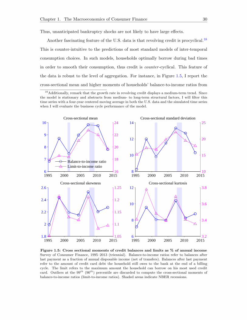
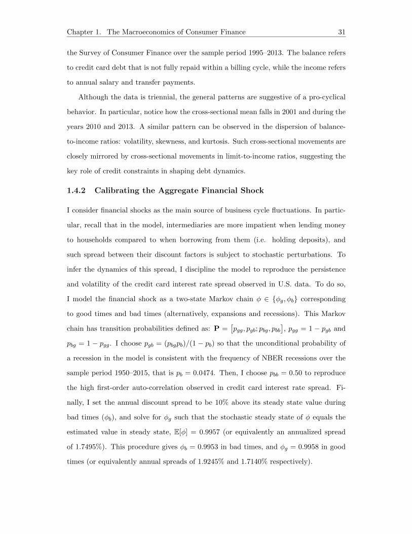
Another fascinating feature of the US data is that revolving credit is procyclical18
This is counter-intuitive to the predictions of most standard models of inter-temporal
consumption choices In such models households optimally borrow during bad times
in order to smooth their consumption thus credit is counter -cyclical This feature of
the data is robust to the level of aggregation For instance in Figure 15 I report the
cross-sectional mean and higher moments of householdsrsquo balance-to-income ratios from
18Additionally remark that the growth rate in revolving credit displays a medium-term trend Sincethe model is stationary and abstracts from medium- to long-term structural factors I will filter thistime series with a four-year centered moving average in both the US data and the simulated time serieswhen I will evaluate the business cycle performance of the model
1995 2000 2005 2010 20156
7
8
9
10Cross-sectional mean
16
18
20
22
24
Balance-to-income ratioLimit-to-income ratio
1995 2000 2005 2010 20158
10
12
14Cross-sectional standard deviation
10
15
20
25
1995 2000 2005 2010 201518
2
22
24
26Cross-sectional skewness
105
11
115
12
125
1995 2000 2005 2010 20156
8
10
12Cross-sectional kurtosis
32
34
36
38
Figure 15 Cross sectional moments of credit balances and limits as of annual incomeSurvey of Consumer Finance 1995ndash2013 (triennial) Balance-to-income ratios refer to balances afterlast payment as a fraction of annual disposable income (net of transfers) Balances after last paymentrefer to the amount of credit card debt the household still owes to the bank at the end of a billingcycle The limit refers to the maximum amount the household can borrow on his most used creditcard Outliers at the 99th (90th) percentile are discarded to compute the cross-sectional moments ofbalance-to-income ratios (limit-to-income ratios) Shaded areas indicate NBER recessions
Chapter 1 The Macroeconomics of Consumer Finance 31
the Survey of Consumer Finance over the sample period 1995ndash2013 The balance refers
to credit card debt that is not fully repaid within a billing cycle while the income refers
to annual salary and transfer payments
Although the data is triennial the general patterns are suggestive of a pro-cyclical
behavior In particular notice how the cross-sectional mean falls in 2001 and during the
years 2010 and 2013 A similar pattern can be observed in the dispersion of balance-
to-income ratios volatility skewness and kurtosis Such cross-sectional movements are
closely mirrored by cross-sectional movements in limit-to-income ratios suggesting the
key role of credit constraints in shaping debt dynamics
142 Calibrating the Aggregate Financial Shock
I consider financial shocks as the main source of business cycle fluctuations In partic-
ular recall that in the model intermediaries are more impatient when lending money
to households compared to when borrowing from them (ie holding deposits) and
such spread between their discount factors is subject to stochastic perturbations To
infer the dynamics of this spread I discipline the model to reproduce the persistence
and volatility of the credit card interest rate spread observed in US data To do so
I model the financial shock as a two-state Markov chain φ isin φg φb corresponding
to good times and bad times (alternatively expansions and recessions) This Markov
chain has transition probabilities defined as P =[pgg pgb pbg pbb
] pgg = 1 minus pgb and
pbg = 1 minus pgg I choose pgb = (pbgpb)(1 minus pb) so that the unconditional probability of
a recession in the model is consistent with the frequency of NBER recessions over the
sample period 1950ndash2015 that is pb = 00474 Then I choose pbb = 050 to reproduce
the high first-order auto-correlation observed in credit card interest rate spread Fi-
nally I set the annual discount spread to be 10 above its steady state value during
bad times (φb) and solve for φg such that the stochastic steady state of φ equals the
estimated value in steady state E[φ] = 09957 (or equivalently an annualized spread
of 17495) This procedure gives φb = 09953 in bad times and φg = 09958 in good
times (or equivalently annual spreads of 19245 and 17140 respectively)
Chapter 1 The Macroeconomics of Consumer Finance 32
Table 15 OLS Coefficients of the Conditional Employment Forecasting Rules
The OLS regression is log πprime = α0 + α1dprime + α2 log π + α3d
prime log π + ε In the model the dummy d takesthe value 1 if φ = φb and 0 otherwise (φ = φg) In the US data the dummy d takes the value 1 if thequarter is a recession as defined by the NBER and 0 otherwise (quarter is an expansion) The USdata covers the sample 1948Q1ndash2015Q2 Uenmployment data is from BLS In the model the samplecovers 1100 quarters (the first 100 quarters are discarded)
Coefficient estimates
α0 α1 α2 α3
Data minus0000546 minus0001789 0968837 0097310Model minus0001114 minus0002667 0960753 0079831
143 Approximate Aggregation in the Model and in US Data
Following Krusell and Smith (1998) I solve for an approximate-aggregation equilibrium
of the model by guessing that households only use current employment rate (π) to
forecast next-quarter employment (πprime) rather than the infinite-dimensional object micro isin
M (household distribution) More formally let d isin 0 1 be a recession dummy variable
that takes the value 1 if φ = φb and 0 otherwise Then consider log-linear forecasting
rules of the form
log πprime = α0 + α1dprime + α2 log π + α3d
prime log π + ε (16)
where ε are the smallest possible forecasting errors made by households in equilibrium
Since households in the model use this forecasting rule to predict employment it is a
pre-requisite of the modelrsquos success that a similar rule-of-thumb could be used in reality
as well The US data-based forecasting rules are visualized in Figure 16 (using postwar
1948Q1ndash2015Q1) Additionally Table 15 compares the OLS parameter estimates of
(16) in the model and in US data It is interesting to notice that the model-based
regression coefficients are in line with the ones based on the data and thus suggests
that approximate aggregation is a reasonable feature of the data
To find the model equilibrium forecasting rules I could solve for the unknown co-
efficients α0 α3 in a guess-and-verify fashion In particular I would simulate an
economy with a given set αlowast0 αlowast3 and make sure that markets clear at each point
in time Then I would run an OLS regression and check whether the forecasting errors
Chapter 1 The Macroeconomics of Consumer Finance 33
ε are small according to some criteria If not I would re-start the process with a new set
of coefficients αlowast0 αlowast3 obtained from OLS Though standard in the literature this
process does not converge in my model because of the high non linearities that default
and unemployment generate
Instead I consider a dual approach Instead of imposing market clearing at each
point in time and checking whether the forecast errors are small I assume that the
economy evolves exactly as predicted by households (thus there are no forecast errors)
and check whether the goods market clear (the magnitude of shortages and excesses)
Thus I do not impose market-clearing ex-interim but only check it ex-post With
this approach an equilibrium is a set of guessed coefficients αlowast0 αlowast3 such that the
89 90 91 92 93 94 95 96 97 9889
90
91
92
93
94
95
96
97
98
Todays employment rate (in )
Nex
t-q
uar
ters
em
plo
ymen
t rat
e (i
n
)
If an expansion occurs next quarterOtherwise if next quarter is a recession
Figure 16 Employment Forecasting Rules in US DataUS data 1948Q1ndash2015Q2 (from BLS) The data is sorted in two groupsldquonext quarter is an expan-sionrdquo and ldquonext quarter is a recessionrdquo according to the NBER dates The forecasting rules are froman Ordinary Least Squares log-linear model log πprime = minus0000546 + minus0001789dprime + 0968837 log π +0097310dprime log π + ε where d isin 0 1 are recession dummies and π corresponds to the employmentrate
Chapter 1 The Macroeconomics of Consumer Finance 34
excesses and shortages in the goods market are the smallest possible Such excesses
and shortages are simply given by the difference between the guessed employment rate
π (production-based) and the one that would have been required to exactly satisfy all
the consumption needs of the households and the government (consumption-based)
Figure 17 plots the employment forecasting rules (production path) against total
actual consumption (expressed in employment units) Each vertical segment represents
the magnitude of either a shortage (if above the production path) or an excess (if
below) In equilibrium the average excesses (shortages) represent only 01673 of the
total quantities produced while the maximum difference is 07135 and occurs mostly
during recessions Such errors are well within the range of the noise observed in the data
89 90 91 92 93 94 95 96 97 9888
89
90
91
92
93
94
95
96
97
98
Todays employment rate (in )
Nex
t qu
arte
rs e
mp
loym
ent r
ate
(in
)
If an expansion occurs next quarterOtherwise if next quarter is a recession
Excess of goods
Shortage of goods
Figure 17 Excesses and Shortages of Goods in the Stochastic General EquilibriumThe two diagonal lines are the equilibrium production paths πprimes = Γ(πs φ
prime) log πprimes = minus0001114 +minus0002667dprime+ 0960753 log πs + 0079831dprime log πs + ε Each vertical line represent the distance betweenwhat is produced (πs) and the employment rate that would be required to satisfy all the public andprivate consumption (πd) The shorter the vertical lines the small the excesses or shortages in thegoods market and hence the closer is the economy to market clearing
Chapter 1 The Macroeconomics of Consumer Finance 35
Table 16 Unemployment and Consumer Finance Statistics Over the Business Cycle
US data 1990Q1ndash2015Q2 Model statistics refer to a sample of one million households simulatedover 1100 quarters and the first 100 quarters are discarded The model frequency is quarterly Thegrowth rates of revolving credit and unsecured leverage display a medium-term cycle that is filteredwith a four-year centered moving average For consistency a similar filtering is applied to the model-generated time series of revolving credit growth and unsecured leverage growth As expected suchfiltering on stationary time series has virtually no quantitative effect The bankruptcy rate (Chapter7 filings divided by civilian population) and the credit card interest rate spread (average credit cardinterest rate minus effective Fed funds rate) are annualized
First-order Corr withMean Volatility auto-corr unemployment
Variables (all in ) Data Model Data Model Data Model Data Model
Unemployment rate 611 582 157 163 098 099 100 100Credit card spread 1128 1061 169 112 096 091 078 095Bankruptcy rate 038 052 013 007 071 031 minus004 034Charge-off rate 487 278 169 038 093 033 051 047Revolving credita minus001 000 109 101 035 024 minus031 minus013Leveragea 001 000 132 096 005 010 minus021 minus013
aDetrended growth rate
and thus should not dramatically affect the main conclusions of the paper As models
of incomplete markets add more frictions and non-linearities this approach offers an
interesting and simple alternative to the standard methods
144 The Joint Dynamics of Consumer Finance and Unemployment
Table 16 presents the main business cycle results of the paper
The credit spread dynamics are relatively well matched In particular it is highly
volatile though it understates the data (112 compared to 169) It is also very persistent
the first-order auto-correlation coefficient is 096 in the data and 091 in the model
Lastly the credit card spread co-moves strongly with the cycle especially more in the
model than in the data the correlation between unemployment and the spread is 095
and 078 respectively
Under this calibration the model replicates salient features of the joint dynamics of
employment and other key financial variables that pertain to unsecured consumer credit
markets growth rate of revolving credit growth rate of the ratio of revolving credit to
aggregate disposable income (which I will refer as unsecured leverage) bankruptcy rate
Chapter 1 The Macroeconomics of Consumer Finance 36
under Chapter 7 and to some extent the charge-off rate on credit cards
The model reproduces the weak correlation between the charge-off rate and unem-
ployment (051 in data 047 in model) and to some extent between the bankruptcy rate
and unemployment (minus004 in data 034 in model) However the model falls short in
explaining the large persistence of such time series (071 and 093 versus 031 and 033)
As a consequence the model also tends to understate the volatility of bankruptcies
and charge-offs (007 compared to 013 and 038 compared 169) The low volatility of
charge-offs is also due to the fact that in steady state their mean is halved Adjusting
for the mean the model-based coefficient of variation is 13 compared to 35 in the
data A way of improving the model fit would be to focus on elements that increase the
persistence of bankruptcies For example I would conjecture that modeling persistent
labor income shocks (as opposed to purely transitory in the current model) could help
along this dimension but at the expense of a more demanding numerical method
Turning to growth rates of revolving credit and unsecured leverage the model ac-
counts well for all of their dynamic properties For instance their volatilities are 109
and 101 respectively in the data compared to 101 and 096 in the model They are
also weakly persistent especially unsecured leverage more than revolving credit 005
and 035 respectively in the data and 010 and 024 in the model Additionally the
model can rationalize the pro-cyclicality of revolving credit and unsecured leverage the
contemporaneous correlations between unemployment and these two series are minus031
and minus021 in the data compared to minus013 and minus013 in the model
Overall the model provides a fair quantitative account of the joint dynamics of
employment and household financial variables
145 The Mechanism at Play From Cross-Sectionial to Aggregate
Since in the model unemployment fluctuations mirror movements in consumption it is
interesting to examine what part of the household distribution drives the business cycle
dynamics To understand the mechanism at play I simulate an economy that recovers
from a one-quarter recession At each point in time I sort households by consumption
Chapter 1 The Macroeconomics of Consumer Finance 37
0 10 20 30 40-05
-04
-03
-02
-01
0Employment impulse response
d
evia
tion
from
initi
al d
ate
0 10 20 30 40-15
-1
-05
0Consumption response by quintile
Q5Q4Q3Q2Q1
0 10 20 30 40-2
-1
0
1
2
d
evia
tion
from
initi
al d
ate
Net worth by consumption quintile
0 10 20 30 40-1
-08
-06
-04
-02
0Income by consumption quintile
Q5Q4Q3Q2Q1
0 10 20 30 40
-8
-6
-4
-2
0
Quarters
d
evia
tion
from
initi
al d
ate
Balance by consumption quintile
0 10 20 30 40-5
0
5
10
15
Quarters
Interest rate by consumption quintile
Q2Q1
Figure 18 Impulse Response Functions by Consumption QuintileEconomic characteristics are obtained by averaging across all the households who belong to the samequintile The first quintile corresponds to households whose consumption is below the 20th percentilethe second quintile to households between the 20th and the 40th percentile and so on The numbers referto Monte Carlo averages of 5 million households over 500 trials The simulated economy experiencesa one-quarter recession at time t = 0 and then remains on an expansionary path for the remainingperiods At each point in time households are sorted by consumption quintile and several averageeconomic characteristics are computed
Chapter 1 The Macroeconomics of Consumer Finance 38
Table 17 Household Economic Characteristics by Consumption Quintile in Steady State
Economic characteristics are obtained by averaging across all households who belong to the same quin-tile The first quintile correspond to households whose consumption is below the 20th percentile thesecond quintile to households between the 20th and the 40th percentile and so on The numbers referto Monte Carlo averages of 5 million households over 500 trials
Sorted by consumption quintile
Average characteristics 1st 2nd 3rd 4th 5th
Consumption 064 071 075 077 082Net worth 028 064 091 121 180Disposable income 057 068 074 080 089Old balance 029 004 minus016 minus041 minus091New balance 036 007 minus016 minus044 minus099Interest rate (annual ) 290 195 059 059 059Default rate (annual ) 088 000 000 000 000
quintile and record their economic characteristics such as income net worth debt
interest paid and default rate
Table 17 reports the averaged household characteristics by consumption quintile
before the economy enters a recession while Figure 18 shows how the different house-
hold groups by consumption quintile fare after the economy experienced a one-quarter
recession
The households in the first two consumption quintiles correspond to borrowers with
low income The borrowers in the first quintiles are particularly indebted likely to
default and face substantial interest rates On the other hand households in the third
fourth and fifth consumption quintile are savers with high income
The key insight of these cross-sectional impulse response functions is that the biggest
drop in consumption comes from the first quintile that is the group of households with
low income and high levels of debt In particular the drop is almost as twice as large
in the first quintile as in any other quintiles
The second key insight is that even the wealthiest households those in the first con-
sumption quintile group slowly build up precautionary savings and consequently hold
back on consumption Notice in particular how their credit balance impulse response
(savings) is hump shaped In opposite the credit balance impulse response of the most
Chapter 1 The Macroeconomics of Consumer Finance 39
Table 18 Consumption Insurance by Net Worth Quintile Over the Business Cycle
I simulate a sample of one million households for 1100 quarters (the first 100 are discarded) At eachpoint in time I sort households by net worth quintiles j = 1 5 For each quintile group I then runthe OLS regression ∆ logCijt = λjt∆ log Υijt + εijt where ∆ logCijt and ∆ log Υijt are log-growthrates of consumption and disposable income respectively and εijt is an error term The table belowpresents the average value of this elasticity across net worth groups over the business cycle as well astheir volatility and correlation with recession dummies dt The recession dummy takes the value 1 ifthe financial shock is φ = φb (bad times) and 0 otherwise
Net worth quintile j =
1 2 3 4 5
E[λjt|j] 01303 00801 00634 00514 00400std(λjt|j) 00047 00020 00012 00008 00005corr(λjt dt|j) 06039 03430 02442 01249 minus00054
credit-constrained households is monotonic in the aftermath of a recession
146 Welfare Implications Procyclical Consumption Insurance
I complete my analysis of the cross-sectional effects of consumer finance disturbances
by measuring the degree of consumption insurance across time periods and households
There are two key implications of the model that I want to highlight First re-
gardless of business cycle fluctuations there is a large cross-sectional heterogeneity in
risk-sharing opportunities This stems from the fact that the lower the net worth of
the household the costlier it is to obtain new loans Therefore households with low or
negative net worth fare worse than wealthy households with high net worth Second
the cross-sectional dispersion in consumption insurance is time-varying This is because
during a recession not only unemployment increases but it is also more difficult to bor-
row for poor households because of higher credit risk Thus households have a lower
ability to smooth their income shocks exactly at the same time when shocks are larger
and more frequent In opposite wealthy households do significantly suffer less during a
recession since they smooth consumption by using precautionary savings
To test these predictions I simulate an economy subject to aggregate shocks At
each point in time I sort households by net worth quintile j = 1 5 Then for each
group j I run the regression
∆ logCijt = λjt∆ log Υijt + εijt
Chapter 1 The Macroeconomics of Consumer Finance 40
where ∆ logCijt and ∆ log Υijt are log-growth rates of consumption and disposable in-
come respectively and εijt is an error term The parameter λjt has the interpretation
of the income elasticity of consumption and measures the degree of consumption insur-
ance As λjt rarr 0 the households who belong to the j-th net worth quintile group at
time t are close to full insurance Table 18 presents the results of this simulation
The first row of the table reports the average income elasticity of consumption by net
worth quintile over the business cycle The cross-sectional dispersion in consumption
is large the top 80 has an elasticity more than three times smaller than the bottom
20 (004 compared to 013) This means that a 10 fall in income results in only 04
consumption fall for the wealthiest households This stems from the fact that they
have large stocks of savings that they can use to smooth consumption In opposite the
poorest households have low or negative net worth and thus can only borrow to smooth
income shocks A 10 fall in income translates in a 13 fall in consumption
The second row of the table reports the volatility of the income elasticity of con-
sumption across time periods Notice that not only the degree of consumption insurance
is low among the poorest but it is also the most volatile and countercyclical Indeed the
third row of the table reports the correlation between λjt and the recession dummy dt
The recession dummy takes the value 1 if the financial shock is φ = φb (bad times) and
0 otherwise The volatility of the income elasticity of consumption is almost 10 times
smaller among the top 80 compared to the bottom 20 Furthermore the fluctua-
tions are acyclical among the richest households the degree of consumption insurance
among the richest households is not correlated with the amount of labor risk they face
In opposite the degree of consumption insurance is strongly correlated with the cycle
among the poorest households (correlation of 060 with the recession dummy dt) Thus
the model generates pro-cyclical consumption insurance among the poorest households
147 Discussion
The take away from these results is that in presence of credit frictions (market incom-
pleteness financial intermediation and risk of default) the actions of borrowers and
Chapter 1 The Macroeconomics of Consumer Finance 41
savers do no longer wash out at the aggregate level The key reason put forth in my
paper is that what is saved by some households is not one-to-one redistributed to other
households in the form of loans For example think of the extreme case when some
households save but credit risk is so high that not a single borrower can obtain a loan
This inefficiency in credit markets has real consequences Since savers do not consume
all their income and credit-constrained borrowers cannot consume as much as they
would want to the overall consumption is lower than what would be required to reach
full employment
Hence this paper provides an unemployment theory purely based on market incom-
pleteness financial intermediation and risk of default rather than traditional frictions
like price stickiness or search
This business cycle theory of consumer finance and unemployment offers new per-
spectives on the effects of government stimulus policies Indeed by viewing unemploy-
ment as a symptom of limited consumption insurance as evidenced in the section above
we can think of stimulus policies that aim at improving risk-sharing among households
Through the lens of the model this means that for example an unemployment insurance
program though having negative effects on the labor supply because of search effects
has also positive effects through improving risk-sharing Similarly a household bailout
policy could be beneficial since it would ease the pressure on poor households who have
a low net worth More broadly any risk-related policy such as a medical insurance
policy or regulations in the credit card markets could prove to be useful in the context
of reducing unemployment Of course each policy would require a careful cost-benefit
analysis in a well structurally estimated model By proposing a simple model that links
unemployment to the degree of consumer credit frictions this paper makes a first step
toward this goal
15 Conclusion
I have developed a dynamic incomplete-market general equilibrium model where house-
holds can hold unsecured debt and production is based on labor I estimated the model
Chapter 1 The Macroeconomics of Consumer Finance 42
parameters in steady state by matching a large set of aggregate and cross sectional
moments Turning to business cycle analysis I have shown that the model matches well
the joint dynamics of unemployment and some key consumer finance statistics In fu-
ture research the model could be used to assess the costs and benefits of some stimulus
policies such as a bailout of highly levered households
The model could also be extended along several lines In particular intermediaries
could be modeled as risk-averse households who solve their own optimization problem
Such extension would allow the model to shed light on the cyclical movements of the
risk-free rate and risk premia Also permanent idiosyncratic shocks could be added to
study the interaction between heterogeneity in leverage and wealth Lastly the model
could be extended to account for capital accumulation in order to study the effects of
consumer finance on a broader set of business cycle statistics
Chapter 2
Misallocation Cycles
21 Introduction
A large body of research has shown that the cross-section of firms is characterized
by a substantial degree of productivity and capital heterogeneity (eg Eisfeldt and
Rampini (2006)) While the empirical facts about firm heterogeneity are well known
the aggregate consequences are not well understood In this paper we develop and
estimate a simply general equilibrium model to illustrate how the dynamics of the cross-
section of firms impact aggregate fluctuations and risk premia via the misallocation
of capital resources The key implication of our general equilibrium model is that
idiosyncratic shocks do not integrate out at the aggregate level but instead generate
cyclical movements in the higher moments of consumption growth and risk premia
Our model is driven by a cross-section of heterogenous firms which face irreversible
investment decisions exit and permanent idiosyncratic and aggregate productivity
shocks The representative household has recursive preferences and consumes aggre-
gate dividends To generate aggregate consequences from a continuum of idiosyncratic
shocks via capital misallocation our model mechanism requires both a power law dis-
tribution as well as common idiosyncratic skewness in productivity
While most of the literature assumes a log-normal idiosyncratic productivity distri-
bution arising from mean-reverting Gaussian shocks idiosyncratic shocks are permanent
and follow random walks in our model With firm exit distributions of random walks
generate power laws as emphasized by Gabaix (1999) and Luttmer (2007) Quantita-
43
Chapter 2 Misallocation Cycles 44
tively the endogenous power law for firm size is consistent with the data as reported in
Axtell (2001) such that the largest 5 of firms generate more than 30 of consumption
and output in our model
In addition to the random walk assumption we model innovations to idiosyncratic
productivity not only with Gaussian but also with negative Poisson shocks which induce
common idiosyncratic skewness These negative Poisson shocks do not capture rare
aggregate disaster as in Gourio (2012) because they wash out at the aggregate level
in a frictionless model1 Instead time variation in the size of common idiosyncratic
skewness allows us to capture the cyclicality in the skewness of cross-sectional sales
growth consistent with the evidence in Salgado et al (2015)
In the model these features lead to large occasional inefficiencies in the allocation
of capital across firms and it hinders the representative agentrsquos ability to smooth con-
sumption Intuitively in recessions aggregate productivity falls and the distribution
of output growth becomes negatively skewed Firms with negative idiosyncratic pro-
ductivity draws are constrained because they cannot disinvest unproductive capital to
raise dividends At the same time the representative household would like to reallocate
capital to smooth consumption
Because of the power law distribution in firm size the share of output coming from
large firms contributes disproportionally to aggregate consumption so that negatively
skewed shocks to their productivity are particularly painful Consequently the drop
in dividends from the mass of constrained is large given that they are large in size
While unconstrained firms increase dividends by reducing investment they are smaller
so that they are not able to offset the impact of large constrained firms on aggregate
consumption This effect implies that in recessions aggregate consumption falls by
more than aggregate productivity causing negative skewness and kurtosis and it arises
purely from the cross-sectional misallocation In contrast in models with log-normal
productivity distributions the size difference between constrained and unconstrained
firms is small so that the groups offset each other
1For disaster risk in consumption see Barro (2006) Gabaix (2012) and Wachter (2013)
Chapter 2 Misallocation Cycles 45
While the impact of capital misallocation on output and consumption are short lived
under temporary mean-reverting shocks permanent Poisson shocks render misalloca-
tion distortions long lasting Quantitatively output and consumption growth become
more volatile and persistent even though the model is only driven iid innovations
Importantly consumption growth is left skewed and leptokurtic as in the data Because
the household cares about long lasting consumption distortions due to Epstein-Zin pref-
erences the welfare costs of capital misallocation and aggregate risk premia are large
Our mechanism to generate aggregate fluctuations from idiosyncratic shocks obeying
a power law is distinct from the granular hypothesis of Gabaix (2011) While Gabaix
also argues that the dynamics of large firms matters for business cycles he relies on
the fact that the number of firms is finite in an economy so that a few very large firms
dominate aggregate output The impact of these very large firms does not wash at the
aggregate level when firm size follows a power law In contrast we model a continuum
of firms so such each individual firm has zero mass In our model the power law in
firm size generates aggregate fluctuations based on capital misallocation arising from
the investment friction and not because the economy is populated by a finite number
of firms In reality both effects are at work to shape business cycles2
Methodologically we build on Veracierto (2002) and Khan and Thomas (2008) who
find that microeconomic investment frictions are inconsequential for aggregate fluctua-
tions in models with mean-reverting idiosyncratic productivity3 We show that a model
with permanent shocks and a more realistic firm size distribution not only breaks this
irrelevance result but also produces risk premia that are closer to the data We are not
the first to model permanent idiosyncratic shocks eg Caballero and Engel (1999) and
Bloom (2009) do so but these paper study investment dynamics in partial equilibrium
frameworks
Starting with the influential paper by Bloom (2009) a growing literature empha-
sizes time varying uncertainty in productivity as driver of business cycles eg Bloom
2Related to the granular notion Kelly et al (2013) derive firm volatility in sparse networks3Bachmann and Bayer (2014) show that the same irrelevance result holds with idiosyncratic volatility
shocks
Chapter 2 Misallocation Cycles 46
et al (2014) Bachmann and Bayer (2014) and Kehrig (2015) We differ from this lit-
erature by focusing on time varying skewness in the cross-section of sales growth It is
well-known that sales growth dispersion is strongly countercyclical Less well-known is
that this countercyclical dispersion is mainly driven by the left tail of the sales growth
distribution By just looking at the cyclicality of the IQR one might conclude that in
recessions firms have more dispersed positive and negative productivity draws But the
cyclicality of Kelly skewness indicates that in recessions significantly more firms have
extreme negative productivity draws Our model is equipped to match this empirical
fact because productivity is not only driven by Gaussian shocks but also by negative
Poisson shocks
This empirical fact is also reminiscent of Guvenen et al (2014) who document that
householdsrsquo income shocks feature procyclical skewness Constantinides and Ghosh
(2015) and Schmidt (2015) show that procyclical skewness is quantitatively important
for aggregate asset prices in incomplete market economies Different from these papers
our paper focuses on heterogeneity on the productive side of the economy and analyzes
the effect of skewed shocks on capital misallocation
The first study to quantify capital misallocation is Olley and Pakes (1996) More
recent contributions include Hsieh and Klenow (2009) and Bartelsman et al (2013) We
extend their measure of capital misallocation and derive a frictionless benchmark in a
general equilibrium framework The importance of capital misallocation for business
cycles is illustrated by Eisfeldt and Rampini (2006)
Our study also relates to the literature on production-based asset pricing including
Jermann (1998) Boldrin et al (2001) and Kaltenbrunner and Lochstoer (2010) which
aims to make the real business cycle model consistent with properties of aggregate asset
prices While these models feature a representative firm we incorporate a continuum
of firms This allows us to pay close attention to cross-sectional aspects of the data
thereby providing a more realistic micro foundation for the sources of aggregate risk
premia While Kogan (2001) and Gomes et al (2003) also model firm heterogeneity
our model provides a tighter link to firm fundamentals such that we estimate model
Chapter 2 Misallocation Cycles 47
parameters
Our model mechanism is also related to the works of Gabaix (1999) and Luttmer
(2007) Gabaix (1999) explains the power law of city sizes with random walks reflected
at a lower bound Using a similar mechanism Luttmer (2007) generates a power law in
firm size in a steady-state model We extend this literature by studying the impact of
a power law in firm size in a business cycle model with common idiosyncratic skewness
shocks
Starting with the influential paper by Berk et al (1999) there exist a large literature
which studies the cross-section of returns in the neoclassical investment framework eg
Carlson et al (2004) Zhang (2005) Cooper (2006) and Gomes and Schmid (2010b)
For tractability these papers assume an exogenous pricing kernel and link firm cash
flows and the pricing kernel directly via aggregate shocks In contrast we provide a
micro foundation for the link between investment frictions and aggregate consumption
22 Model
Time is discrete and infinite The economy is populated by a unit mass of firms Firms
own capital produce output with a neoclassical technology subject to an investment
irreversibility constraint and face permanent idiosyncratic and aggregate shocks The
representative household has recursive preferences and consumes aggregate dividends
This section elaborates on these model elements and defines the recursive competitive
equilibrium of the economy
221 Production
Firms produce output Y with the neoclassical technology
Y = (XE)1minusαKα (21)
where X is aggregate productivity E is idiosyncratic productivity K is the firmrsquos capital
stock and α lt 1 is a parameter that reflects diminishing returns to scale Aggregate
productivity X follows a geometric random walk
X prime = expgx minus σ2x2 + σxη
primex
X (22)
Chapter 2 Misallocation Cycles 48
where gx denotes the average growth rate of the economy σx the volatility of log aggre-
gate productivity growth and ηx an iid standard normal innovation
Idiosyncratic productivity growth is a mixture of a normal and a Poisson distribu-
tion allowing for rare but large negative productivity draws These negative jumps
capture for instance sudden drops in demand increases in competition the exit of
key human capital or changes in regulation As we will see they are also essential for
allowing the model to replicate the cross-sectional distribution of firmsrsquo sales growth
Specifically idiosyncratic productivity E follows a geometric random walk modulated
with idiosyncratic jumps
E prime = expgε minus σ2ε2 + σεη
primeε + χprimeJ prime minus λ
(eχprime minus 1
)E (23)
where gε denotes the average firm-specific growth rate σε the volatility of the normal
innovations in firm-specific productivity η an iid idiosyncratic standard normal shock
and J an iid idiosyncratic Poisson shock with constant intensity λ The jump size χ
varies with aggregate conditions ηx which we capture with the exponential function
χ(ηx) = minusχ0eminusχ1ηx (24)
with strictly positive coefficients χ0 and χ1 This specification implies that jumps are
negative and larger in worse aggregate times ie for low values of ηx Our specification
for idiosyncratic productivity warrants a few comments
First Bloom (2009) structurally estimates the cyclicality in the dispersion of idiosyn-
cratic productivity which is a symmetric measure of uncertainty Our specification also
leads to time variation in the higher moments of idiosyncratic productivity growth In
particular equation (24) implies that firm-specific productivity shocks become more
left skewed in recessions Second different from the uncertainty shocks in Bloom (2009)
and Bloom et al (2014) our assumptions imply that changes in idiosyncratic jump risk
are neither known to firms ex ante nor persistent and therefore do not cause wait-and-
see effects As we will show however they induce large changes in measured aggregate
productivity via their effect on the efficiency of the cross-sectional capital distribution
Third in contrast to the consumption based asset pricing literature with disaster risk in
Chapter 2 Misallocation Cycles 49
consumption for instance Barro (2006) Gabaix (2012) and Wachter (2013) we do not
model time variation in the jump probability λ If the jump probability were increasing
in recessions it would induce rising skewness in productivity and sales growth while
in the data it is falling4 Fourth the idiosyncratic jump risk term χJ is compensated
by its mean λ(eχ minus 1) so that the cross-sectional mean of idiosyncratic productivity is
constant (see equation (25) below) This normalization implies that aggregate produc-
tivity is determined solely by ηx-shocks so that our model does not generate aggregate
jumps in productivity as emphasized by eg Gourio (2012) Because the size of the
jump risk is common across firms we refer to it as common idiosyncratic skewness in
productivity
Given the geometric growth in idiosyncratic productivity the cross-sectional mean
of idiosyncratic productivity is unbounded unless firms exit We therefore assume that
at the beginning of a period ndash before production takes place and investment decisions
are made ndash each firm exits the economy with probability π isin (0 1) Exiting firms are
replaced by an identical mass of entrants who draws their initial productivity level from
a log-normal distribution with location parameter g0 minus σ202 and scale parameter σ0
Whenever firms exit their capital stock is scrapped and entrants start with zero initial
capital
Since the idiosyncratic productivity distribution is a mixture of Gaussian and Pois-
son innovations it cannot be characterized by a known distribution5 But two features
are noteworthy First due to random growth and exit the idiosyncratic productivity
distribution and thus firm size features a power law as shown by Gabaix (2009) A
power law holds when the upper tail of the firm size distribution obeys a Pareto distri-
bution such that the probability of size S greater than x is proportional to 1xζ with
tail (power law) coefficient ζ6
Second even though the distribution is unknown we can compute its higher mo-
4Note that skewness of Poisson jumps J equals λminus125Dixit and Pindyck (1994) assume a similar process without Poisson jumps in continuous time and
solve for the shape of the cross-sectional density numerically see their chapter 846In our model the tail coefficient solves the nonlinear equation 1 = (1 minus π)Z(ζ) where Z(ζ) =
expζgε minus ζσ2ε2 + ζ2σ2
ε2 + λ(eζχ minus 1)minus ζλ(eχ minus 1)
Chapter 2 Misallocation Cycles 50
ments Let Mn denote the n-th cross-sectional raw moment of the idiosyncratic pro-
ductivity distribution E It has the following recursive structure
Mprimen = (1minus π) expngε minus nσ2ε2 + n2σ2ε2 + λ(enχprime minus 1)minus nλ(eχ
prime minus 1)Mn (25)
+π expng0 minus nσ202 + n2σ202
The integral over idiosyncratic productivity and capital determines aggregate out-
put To ensure that aggregate output is finite we require that the productivity distri-
bution has a finite mean7 Equation (25) states that the mean evolves according to
Mprime1 = (1minus π)egεM1 + πeg0 which is finite if
gε lt minus ln(1minus π) asymp π (26)
In words the firm-specific productivity growth rate has to be smaller than the exit rate
In this case the first moment is constant and for convenience we normalize it to one
by setting
g0 = ln(1minus egε(1minus π))minus ln(π) (27)
222 Firms
To take advantage of higher productivity firms make optimal investment decisions
Capital evolves according to
K prime = (1minus δ)K + I (28)
where δ is the depreciation rate and I is investment As in Khan and Thomas (2013)
and Bloom et al (2014) we assume investment is partially irreversible which generates
spikes and positive autocorrelation in investment rates as observed in firm level data
Quadratic adjustment costs can achieve the latter only at the expense of the former
since they imply an increasing marginal cost of adjustment Partial irreversibility means
that firms recover only a fraction ξ of the book value of capital when they choose to
disinvest These costs arise from resale losses due to transactions costs asset specificity
and the physical costs of resale
7Luttmer (2007) makes a related assumption (Assumption 4) which states that ldquoa firm is notexpected to grow faster than the population growth raterdquo to ensure that the firm size distribution hasfinite mean
Chapter 2 Misallocation Cycles 51
We show in Section 23 that partial irreversibility yields an (Ss) investment policy
such that firms have nonzero investment only when their capital falls outside an (Ss)
inactivity band8 A firm with an unacceptably high capital stock relative to its cur-
rent productivity will reduce its stock only to the upper bound of its inactivity range
Similarly a firm with too little capital invests only to the lower bound of its inactivity
range to reduce the linear penalty it will incur if it later chooses to shed capital Thus
partial irreversibility can deliver persistence in firms investment rates by encouraging
repeated small investments at the edges of inactivity bands
We summarize the distribution of firms over the idiosyncratic states (K E) using
the probability measure micro and note that the aggregate state of the economy is given by
(Xmicro) The distribution of firms evolves according to a mapping Γ which we derive in
Section 23 Intuitively the dynamics of micro are shaped by the exogenous dynamics of E
and X the endogenous dynamics of K resulting from firmsrsquo investment decisions and
firm entry and exit
Firms maximize the present value of their dividend payments to shareholders by
solving
V (K E X micro) = maxI
D + (1minus π)E
[M primeV (K prime E prime X prime microprime)
] (29)
where
D = Y minus I 1Ige0 minus ξI 1Ilt0 (210)
denotes the firmrsquos dividends and M is the equilibrium pricing kernel based on aggregate
consumption and the householdrsquos preferences which we derive in Section 231
223 Household
The representative household of the economy maximizes recursive utility U over con-
sumption C as in Epstein and Zin (1989a)
U(Xmicro) = maxC
(1minus β)C1minus 1
ψ + β(E[U(X prime microprime)1minusγ
])(1minus 1
ψ)(1minusγ)
1(1minus 1
ψ)
(211)
where ψ gt 0 denotes the elasticity of intertemporal substitution (EIS) β isin (0 1) the
subjective discount factor and γ gt 0 the coefficient of relative risk aversion In the
8See Andrew B Abel (1996) for a continuous time model of partial irreversibility
Chapter 2 Misallocation Cycles 52
special case when risk aversion equals the inverse of EIS the preferences reduce to the
common power utility specification The householdrsquos resource constraint is
C =
intD dmicro (212)
224 Equilibrium
A recursive competitive equilibrium for this economy is a set of functions (CU VKΓ)
such that
(i) Firm optimality Taking M and Γ as given firms maximize firm value (29) with
policy function K subject to (28) and (210)
(ii) Household optimality Taking V as given household maximize utility (211) sub-
ject to (212) with policy function C
(iii) The good market clears according to (212)
(iv) Model consistency The transition function Γ is induced by K aggregate produc-
tivity X equation (22) idiosyncratic productivity E equation (23) and entry
and exit
23 Analysis
In this section we characterize firmsrsquo optimal investment policy and the transition dy-
namics of the cross-sectional distribution of firms We also derive closed-form solutions
for a frictionless version of the model which serves an a benchmark for quantifying the
degree of capital misallocation and the wedge between actual and measured aggregate
productivity Because aggregate productivity contains a unit root we solve the model
in detrended units such that detrended consumption c and wealth w are given by
c = CX w = WX
231 Household Optimization
The householdrsquos first order condition with respect to the optimal asset allocation implies
the usual Euler equation
E[M primeRprime
]= 1 (213)
Chapter 2 Misallocation Cycles 53
where M prime is the pricing kernel and Rprime is the return on equity defined by V prime(V minusD)
The pricing kernel is given by
M prime = βθ(xprime)minusγ(cprime
c
)minusθψ ( wprime
w minus c
)θminus1 (214)
where θ = 1minusγ1minus1ψ is a preference parameter and xprime = X primeX is iid log-normal dis-
tributed In the case of power utility θ equals one and wealth drops out of the pricing
kernel With Epstein-Zin preferences the dynamics of both consumption and wealth
evolve endogenously and are part of the equilibrium solution
Consistent with the Euler equation (213) wealth is defined recursively as the present
value of future aggregate consumption
w = c+ βE
[(xprime)1minusγ(wprime)θ
(cprime
c
)minusθψ]1θ (215)
Firm exit introduces a wedge between wealth and the aggregate market value of firms
This stems from the fact that wealth captures the present value of both incumbents
and entrants whereas aggregate firm value relates to the present value of dividends of
incumbent firms only
232 Firm Optimization
Having solved for the functional form of the pricing kernel we can characterize firmsrsquo
optimal investment policy The homogeneity of the value function and the linearity of
the constraints imply that we can detrend the firm problem by the product of both
permanent shocks XE as for instance in Bloom (2009) We define the firm-specific
capital to productivity ratio κ = K(XE) the capital target to productivity ratio
τ = K prime(XE) and the firm value to productivity ratio v = V(XE)
Given the linear cost structure one can divide the value function into three regions
In the investing region ((1 minus δ)κ le τ) firms increase their capital to productivity
ratio and the optimal firm value solves vu in the disinvesting region (τ le (1 minus δ)κ)
firms decrease their capital to productivity ratio and the optimal firm value solves vd
otherwise firms are inactive Firm value v is thus the maximum of the value of investing
Chapter 2 Misallocation Cycles 54
vu disinvesting vd or inactivity
vu(κ micro) = max(1minusδ)κleτ
κα minus (τ minus (1minus δ)κ) + (1minus π)E
[M primexprimeεprimev
(κprime microprime
)] (216)
vd(κ micro) = maxτle(1minusδ)κ
κα minus ξ(τ minus (1minus δ)κ) + (1minus π)E
[M primexprimeεprimev
(κprime microprime
)] (217)
v(κ micro) = maxvu(κ micro) vd(κ micro) κα + (1minus π)E
[M primexprimeεprimev
((1minus δ)κ(xprimeεprime) microprime
)](218)
where εprime = E primeE Because both growth rates εprime and xprime are iid the state space of
the detrended firm problem reduces to (κ micro) Importantly for adjusting firms next
periodrsquos capital to productivity ratio κprime = τ(xprimeεprime) is independent of the current capital
to productivity ratio This fact implies that firms share a common time-varying capital
target τ which is independent of their own characteristic κ The optimal capital targets
for the investing and disinvesting regions is given by Tu(micro) and Td(micro) respectively and
solves
Tu(micro) = arg maxτ
minusτ + (1minus π)E
[M primexprimeεprimev
(τ(xprimeεprime) microprime
)]
Td(micro) = arg maxτ
minusξτ + (1minus π)E
[M primexprimeεprimev
(τ(xprimeεprime) microprime
)]
Given these capital targets the optimal policy of the firm-specific capital to productivity
ratio can be characterized by an (S s) policy and is given by
κprime = maxTu(micro)minTd(micro) (1minus δ)κ
(xprimeεprime) (219)
where the max operator characterizes the investing region and the min operator the
disinvesting one Conditional on adjusting the capital to productivity ratio of every
firm is either Tu or Td independent of their own characteristic κ but dependent on the
aggregate firm distribution micro
The optimal investment rate policy implied by (219) can be summarized by the
same thee regions of investment inactivity and disinvestment
I
K=
Tu(micro)minusκ
κ + δ (1minus δ)κ lt Tu investing
0 Tu le (1minus δ)κ le Td inactive
Td(micro)minusκκ + δ Td lt (1minus δ)κ disinvesting
Chapter 2 Misallocation Cycles 55
In Figure 21 we plot both the optimal capital to productivity and investment rate
policies for two arbitrary capital targets Intuitively when a firm receives a positive
idiosyncratic productivity draw its capital to productivity ratio κ falls If the shock is
large enough and depreciated κ is less than Tu it will choose a positive investment rate
which reflects the relative difference between target and current capital to productivity
ratio as well as the depreciation rate As a result next periodrsquos capital to productivity
ratio will reach Tu in the investment region
When a firm experiences an adverse idiosyncratic productivity draw its capital to
productivity ratio κ increases and it owns excess capital If the shock is severe enough
and depreciated κ is greater than Td it will choose a negative investment rate which
reflects the relative difference between target and current capital to productivity ratio
as well as the depreciation rate As a result next periodrsquos capital to productivity ratio
will fall to Td in the disinvestment region For small enough innovations the depreciated
capital to productivity ratio remains within Tu and Td In this region firms are inactive
and have a zero investment rate
An important features of our model is that there is heterogeneity in the duration of
disinvestment constraintness This feature arises because adverse idiosyncratic produc-
tivity shocks can arise either from a normal distribution or from a Poisson distribution
While adverse normal distributed shocks are short lasting Poisson shocks are rare and
large and therefore long lasting As a result of Poisson shocks the capital to productiv-
ity ratio rises dramatically indicating a long duration of disinvestment constraintness
233 Aggregation
In the previous section we have shown that the firm-specific state space of the firmrsquos
problem reduces to the univariate capital to productivity ratio κ One might therefore
conjecture that the household only cares about the distribution of the capital to produc-
tivity ratio across firms Yet the univariate distribution of the capital to productivity
ratio is not sufficient to solve for equilibrium consumption
Aggregate output is the integral over the product of capital and idiosyncratic pro-
Chapter 2 Misallocation Cycles 56
Current capital to productivity ratio (5)0 02 04 06 08 1 12 14 16 18 2
Nex
tper
iod
capitalto
pro
duct
ivity
ratio
(50 )
0
02
04
06
08
1
12
14
16
18
2
Investing Disinvesting
Inactive Tu
Td
(1 )5 amp
Current capital to productivity ratio (5)0 02 04 06 08 1 12 14 16 18 2
Inves
tmen
tra
te(I
=K
)
-1
-08
-06
-04
-02
0
02
04
06
08
1
Investing
Disinvesting
Inactive
Figure 21 Optimal capital and investment rate policies
ductivity and thus the correlation between capital and idiosyncratic productivity mat-
ters While capital and idiosyncratic productivity are perfectly correlated in the fric-
tionless economy the investment friction renders capital and idiosyncratic productivity
Chapter 2 Misallocation Cycles 57
imperfectly correlated As a result the joint distribution of capital and idiosyncratic
productivity matters for aggregate consumption because it captures the degree of cap-
ital misallocation across firms whereas in the frictionless model aggregate capital is a
sufficient variable for the firm-level distribution
Instead of normalizing capital by both permanent shocks XE we define detrended
capital k by k = KX We can then summarize the distribution of firms over the
idiosyncratic states by (k E) using the probability measure micro which is defined on the
Borel algebra S for the product space S = R+0 timesR+9 The distribution of firms evolves
according to a mapping Γ which is derived from the dynamics of idiosyncratic produc-
tivity E in equation (23) and capital The law of motion for detrended capital can be
obtained by multiplying firmsrsquo optimal policies (219) with idiosyncratic productivity E
and is given by
kprime = maxETu(micro)minETd(micro) (1minus δ)k
xprime (220)
In Figure 22 we illustrate the three regions of micro implied by the optimal capital pol-
icy (220) For the majority of firms capital and idiosyncratic productivity are closely
aligned such that these firms are optimally inactive When idiosyncratic productiv-
ity exceeds capital firms optimally invest such that next periodrsquos capital lies on the
(blue) boundary to inactivity Similarly when capital exceeds idiosyncratic productiv-
ity firms optimally disinvest such that next periodrsquos capital lies on the (red) boundary
to inactivity
Given the capital policy (220) the aggregate resource constraint detrended by X
yields detrended consumption
c =
intE1minusαkα dmicro+(1+ξ)(1minusδ)kminus
intmaxETu (1minusδ)k dmicrominusξ
intminETd (1minusδ)kdmicro
(221)
where k =intk dmicro denotes the aggregate capital stock The first term is aggregate
output the second one is the book value of depreciated capital the third one captures
aggregate investment and the fourth one aggregate disinvestment
9Note that with a slight abuse of notation we continue to use the symbols micro and Γ to denote thedistribution of firms and its transition in the detrended economy
Chapter 2 Misallocation Cycles 58
Log Capital ln(k)-2 -15 -1 -05 0 05 1 15 2
Log
Pro
duct
ivity
ln(E
)
-2
-15
-1
-05
0
05
1
15
2
Investing
Disinvesting
Inac
tive
Figure 22 Optimal capital policies in the micro-distribution
The distribution micro evolves over time according to the mapping Γ (micro ηprimex) 7rarr microprime
To derive this mapping note that the capital policy kprime in equation (220) is predeter-
mined with respect to the firm-level productivity shocks (ηprime J prime) This implies that
conditional on current information and next periodrsquos aggregate shock ηprimex next periodrsquos
characteristics (kprime E prime) are cross-sectionally independent of one another Therefore for
any (KE) isin S
microprime(KE|ηprimex) = microprimek(K|ηprimex)times microprimeE(E|ηprimex) (222)
where microk and microE are the marginal distributions of capital and productivity respectively
The measure of firms with a capital stock of kprime isin K next period is simply the integral
over the measure of firms who choose kprime as their optimal policy this period and survive
plus the mass of entrants in the case 0 isin K
microprimek(K|ηprimex) = (1minus π)
int1kprimeisinK dmicro+ π10isinK (223)
The measure of firms with an idiosyncratic productivity of E prime isin E next period follows
from the fact that conditional on (E J prime ηprimex) E prime is log-normally distributed for continuing
Chapter 2 Misallocation Cycles 59
firms For entrants idiosyncratic productivity is log-normally distributed as well The
distribution of E prime conditional on ηprimex can therefore be computed as follows
microprimeE(E|ηprimex) =
intE primeisinE
(1minus π)
int infinsumj=0
pjφ
ln(E prime)minus(
ln(E) + gε minus σ2ε
2 + χprimej minus λ(eχprime minus 1
))σε
dmicroE
+πφ
(ln(E prime)minus
(g0 minus σ2ε2
)σε
)dE prime (224)
where pj = λjeminusλj is the Poisson probability of receiving j jumps and φ the standard
normal density Equations (222)ndash(224) define the transition function Γ
234 Frictionless Economy
To understand the impact of irreversible investment on aggregate consumption and
output we also solve the frictionless economy as a benchmark This benchmark allows
us to quantify the degree of capital misallocation and to compute the resulting distortion
in output and measured total factor productivity resulting from partial irreversible
investment
Without investment friction the optimal firmsrsquo investment target can be solved for
analytically
T (micro) =
((1minus π)αE[M prime(xprimeεprime)1minusα]
1minus (1minus π)(1minus δ)E[M prime]
)1(1minusα)
and optimal capital capital policy (220) simplifies to
kprime = ET (micro)xprime (225)
Intuitively without the irreversibility constraint firms are at their optimal capital target
in every period
In the frictionless case it is feasible to derive a closed-form expression for the law
of motion of aggregate capital Specifically by aggregating the optimal capital policy
(225) across firms it follows that
kprime = (1minus π)T xprime
Intuitively aggregate capital is a weighted average of the investment target of incum-
bents and average capital of entrants This aggregation result fails in the full model
Chapter 2 Misallocation Cycles 60
Case I Case IIkhigh 0 05 khigh 05 0klow 05 0 klow 0 05
εlow εhigh εlow εhigh
Table 21 Two stylized firm-level distributions
because the optimal capital policy under partial irreversible investment (220) implies
that future capital is a function of past shocks rendering capital and idiosyncratic
shocks correlated
Similarly the detrended aggregate resource constraint (221) in the frictionless econ-
omy simplifies to c = y + (1minus δ)k minus T In contrast to the full model aggregate output
in the frictionless economy collapses to a function of aggregate capital k and is given by
y = A(1minus π)1minusαkα (226)
where A is a Jensen term coming from the curvature in the production function
In the full model capital is misallocated across firms because unproductive firms
find it costly to disinvest We propose three measure of resource misallocation a capital
misallocation measure M an output distortion measure D and measured total factor
productivity Z
The first misallocation measure is the correlation between capital and productivity
M = 1minus Corr(lnK prime ln E) (227)
In the frictionless case capital is never misallocated and M = 0 in each period In the
full model the more capital is misallocated across firms the larger is M
To illustrate capital misallocation in the context of our model we present two styl-
ized firm-level distributions in Table 21 where both idiosyncratic productivity and
capital can only take on two values The table entries are the probability mass for each
point in the support of micro in line with the intuition of Figure 22 In Case I produc-
tive firms hold a high capital stock while unproductive firms hold a low capital stock
Consequently there is no capital misallocation and M = 1 In Case II the scenario is
reversed and capital completely misallocated with M = minus1
Chapter 2 Misallocation Cycles 61
Our capital misallocation measure is similar to the one in Olley and Pakes (1996)
who suggest the covariance between size and productivity This covariance measure has
been used more recently by Hsieh and Klenow (2009) and Bartelsman et al (2013)
While covariances are unbounded the upper bound of our correlation measure has a
simple economic interpretation
The second measure is the output loss due to capital misallocation The output
distortion measure D is defined as the ratio of output in the full model relative to
output on the frictionless economy and is given by
D =
intE1minusαkα dmicro
A(1minus π)1minusαkα (228)
The output distortion measure is tightly linked to our third measure of misallocation
namely measured TFP It is defined as TFP backed out from the full model assuming
that aggregate production can be described as a function of aggregate capital as in
equation (226) and given by Z = XD Interestingly while the log growth rate of true
aggregate TFP is iid and normally distributed measured TFP can feature persistence
in growth rates arising from misallocation
∆ lnZ prime = gx minus σ2x2 + σxηprimex + ∆ lnDprime (229)
235 Numerical Method
As in Krusell and Smith (1998) we approximate the firm-level distribution micro with an
aggregate state variable to make the model solution computable Krusell and Smith
and most of the subsequent literature used aggregate capital k =intk dmicro and higher
cross-sectional moments of capital to summarize the policy-relevant information in micro
Instead we use detrended aggregate consumption c and we argue that this approach is
better suited for models with quantitatively important degrees of capital misallocation
While aggregate capital (and higher moments of capital) depends only on the marginal
distribution of capital consumption depends on the joint distribution of capital and
productivity To illustrate the importance of this feature consider again the stylized
example in Table 21 In both cases the aggregate capital stock equals (klow +khigh)2
Chapter 2 Misallocation Cycles 62
Consumption however will be much higher in Case I where capital is not misallo-
cated and productive firms hold a high capital stock In this case aggregate output is
higher and likely to remain so for the foreseeable future due to the permanent nature
of shocks and the investment friction Therefore consumption is better suited than
aggregate capital for summarizing the economically relevant aspects of micro in our model
We suspect that this advantage carries over to other cross-sectional models that feature
substantial amounts of capital misallocation
Methodologically the main difference between aggregate capital compared to con-
sumption as state variable arises when specifying their law of motions Tomorrowrsquos
capital stock for each firm is contained in the current information set which implies
that tomorrowrsquos aggregate capital stock is contained in the current information set as
well Consequently it is possible to approximate the law of motion for aggregate capital
with a deterministic function On the contrary tomorrowrsquos consumption is not known
today but depends on tomorrowrsquos realization of the aggregate shock ηprimex We approximate
the law of motion for consumption with an affine function in log consumption
ln cprime = ζ0(ηprimex) + ζ1(η
primex) ln c (230)
These forecasting functions imply intercepts and slope coefficients which depend on the
future shock to aggregate productivity ie they yield forecasts conditional on ηprimex As we
illustrate quantitatively in Section 25 this functional form for aggregate consumption is
not very restrictive as it allows for time variation in conditional moments of consumption
growth
In a model based on a representative household with power utility the consumption
rule (230) is sufficient to close the model Because we model a representative household
with recursive utility we also have to solve for the wealth dynamics to be able to compute
the pricing kernel (214) Khan and Thomas (2008) assume that marginal utility of
consumption is a log linear function in aggregate capital and estimate the coefficients
based on simulated data of the model Instead given consumption dynamics (230)
we use the Euler equation for the return on wealth (215) to determine log wealth as
a function log consumption ie w(c) To this end we minimize the Euler equation
Chapter 2 Misallocation Cycles 63
error by iterating on the Euler equation As a result wealth dynamics and optimal
consumption satisfy the equilibrium Euler equation and the model does not allow for
arbitrage opportunities
To summarize our algorithm works as follows Starting with a guess for the co-
efficients of the equilibrium consumption rule (230) we first solve for the wealth rule
and then the firmrsquos problem (216)ndash(218) by value function iteration To update the
coefficients in the equilibrium rule (230) we simulate a continuum of firms Following
Khan and Thomas (2008) we impose market clearing in the simulation meaning that
firm policies have to satisfy the aggregate resource constraint (221) The simulation
allows us to update the consumption dynamics and we iterate on the procedure until
the consumption dynamics have converged
24 Estimation
The main goal of our paper is to relate aggregate fluctuations and risk premia to time
variation in the efficiency of factor allocations at the firm level Because such variation
results from the interplay of idiosyncratic risk and frictions it is crucial for our model
to capture the cyclicality in the shocks that individual firms face We therefore esti-
mate productivity parameters based on a set of moments that reflects both the shape
and cyclicality of the cross-sectional distribution In particular our simulated method
of moments (SMM) estimation targets the cross-sectional distribution of firmsrsquo sales
growth and investment rates along with a set of aggregate quantity moments Our
paper is the first to estimate a general equilibrium model with substantial heterogene-
ity based on such a set of endogenous moments This is made feasible largely due to
modeling shocks as permanent which allows us to reduce the dimensionality of the state
space relative to earlier studies such as Khan and Thomas (2008) Bachmann and Bayer
(2014) or Bloom et al (2014)
Chapter 2 Misallocation Cycles 64
241 Data
Our estimation relies on both aggregate and firm-level data over the period from 1976
to 2014 We use quarterly data but the moments are annual (based on four quarters)
This allows us to make use of the higher information content of quarterly relative to
annual data while avoiding the seasonal variation of quarterly moments
We define aggregate output as gross value added of the nonfinancial corporate sec-
tor aggregate investment as private nonresidential fixed investment and aggregate
consumption as the difference between output and investment All series are per capita
and deflated with their respective price indices Aggregate moments are based on four
quarter log growth rates
Firm-level data is taken from the merged CRSP-Compustat database We eliminate
financial firms (SIC codes 6000-6999) and utilities (SIC codes 4900-4999) because our
model is inappropriate for these firms Additionally we only consider firms with at
least 10 years of data While this filter induces a sample selection bias it also ensures
that the time-variation in cross-sectional statistics is mostly driven by shocks to existing
firms as opposed to changes in the composition of firms In reality such changes are
driven by firmsrsquo endogenous entry and exit decisions but this channel is outside of our
model
We estimate the model based on cross-sectional moments of sales growth and invest-
ment rates Sales growth is defined as the four quarter change in log SALEQ deflated
by the implicit price deflator for GDP The investment rate is defined as the sum of four
quarterly investment observations divided by the beginning capital stock We compute
quarterly investment as the difference in net property plant and equipment (PPENTQ)
deflated by the implicit price deflator for private nonresidential fixed investment10 Cap-
ital is computed using a perpetual inventory method11 The cross-sectional dimension
10This assumes that economic depreciation is equal to accounting depreciation A preferable approachwould be to define investment as the difference in gross PPE and subtract economic depreciation Yetindividual firmsrsquo economic depreciation is not observable
11The perpetual inventory method assumes that Kit = (1minusδ)Kitminus1+Iit initialized using PPENTQdeflated by the implicit price deflator for private nonresidential fixed investment As in our calibrationwe assume a quarterly depreciation rate of δ = 25
Chapter 2 Misallocation Cycles 65
of our final sample grows from 915 firms in the first quarter of 1977 to 1501 firms in the
last quarter of 2014
242 Cyclical Properties of the Cross-Section of Firms
In this section we document how the cross-section of firms moves over the business
cycle and we discuss implication of the associated empirical facts Figure 23 shows
the evolution of the cross-sectional distributions of firmsrsquo sales growth (left column)
and investment rates (right column) over time We summarize both distributions with
robust versions of their first three moments ie we measure centrality with the median
dispersion with the inter quartile range (IQR) and asymmetry with Kelly skewness12
The two top panels of the figure show that recessions are characterized by sizable de-
clines in sales growth and investment rates for the median firm This observation is
unsurprising However recessions are further characterized by pronounced changes in
the shape of the cross-sectional distributions
Sales growth becomes more disperse during recessions and its skewness switches
sign from positive to negative This evidence suggests that recessions coincide with an
increase in idiosyncratic risk Bloom (2009) and Bloom et al (2014) provide ample
additional evidence for the increase in dispersion and model it as an increase in the
volatility of firmsrsquo Gaussian productivity shocks However the pronounced change in
the skewness of sales growth shows that the countercyclicality of idiosyncratic risk is
better described as resulting from an expansion of the left tail of the shock distribution
as opposed to a symmetric widening of the whole distribution Intuitively recessions
are times where a subset of firms receives very negative shocks but it is not the case
that an equal proportion of firms receives very positive shocks
Another characteristic of recessions is the fact ndash first documented by Bachmann and
Bayer (2014) ndash that the dispersion in firmsrsquo investment rates declines This procyclicality
is suggestive of nonconvexities in firmsrsquo capital adjustment cost because in the absence
12Kelly skewness is defined as KSK= (p90minusp50)minus(p50minusp10)p90minusp10
where px denotes the x-th percentile of thedistribution It measures asymmetry in the center of the distribution as opposed to skewness that canresult from tail observations Similar to the median and IQR Kelly skewness is thus robust to outliers
Chapter 2 Misallocation Cycles 66
1980 1990 2000 2010
Med
ian
-02
-01
0
01
02Sales Growth
1980 1990 2000 2010
Inte
r Q
uart
ile R
ange
01
02
03
1980 1990 2000 2010
Kel
lys
Ske
wne
ss
-03
-01
01
03
1980 1990 2000 2010005
01
015
02
025Investment Rate
1980 1990 2000 201001
02
03
1980 1990 2000 2010
0
02
04
06
Figure 23 Robust cross-sectional moments of annual sales growth and investment rates
of such frictions the increase in the dispersion of firmsrsquo productivity would lead to a
larger dispersion in investment rates
Bachmann and Bayer (2014) argue that the same fact is informative about the
cyclicality of idiosyncratic risk In particular they show that a model with uncertainty
shocks and wait-and-see effects in the spirit of Bloom et al (2014) counterfactually
produces a procyclical investment rate dispersion when uncertainty shocks tend to be
large ndash as calibrated by Bloom et al The intuition for this result is that when Gaus-
sian volatility increases during recessions the subset of firms receiving large positive
shocks will undertake large positive investments which leads to an increase in the
cross-sectional dispersion of investment rates When changes in uncertainty are large
enough this effect dominates the real options effect that causes firms to delay their
investments in the face of increased uncertainty which all else equal reduces the dis-
persion in investment rates On the other hand when uncertainty shocks are more
moderately sized the model becomes consistent with the procyclical investment rate
Chapter 2 Misallocation Cycles 67
dispersion but uncertainty shocks no longer induce serious business cycles Bachmann
and Bayer (2014) therefore argue that the countercyclical dispersion of investment rates
places a robust and tight upper bound on degree of countercyclicality of idiosyncratic
risk and they challenge the view advocated by Bloom (2009) and Bloom et al (2014)
that firm level risk shocks are an important driver of business cycles However we note
that this conclusion relies on a model with (a) real option effects and (2) time-variation
in idiosyncratic risk that results from a symmetric change in the dispersion of shocks
Neither of these features are present in our model
243 Simulated Method of Moments
This section explains how we estimate the model parameters The full set of model
parameters includes preference (β γ ψ) technology (δ α) entry and exit (π σ0) and
productivity θ equiv (χ0 χ1 λ gε σε gX σX) parameters Since it is not feasible compu-
tationally to estimate the full set of parameters we focus on estimating the vector of
productivity parameters θ
Values for the remaining parameters are taken from previous literature and are
shown in Panel A of Table 22 Following Bansal and Yaron (2004) we assume that the
representative agent is fairly risk averse γ = 10 and has a large EIS ψ = 2 The time
discount rate of β = 0995 is chosen to achieve a low average risk-free rate Capital
depreciates at a rate of 25 and the curvature of the production function equals 065
similar to Cooper and Haltiwanger (2006) Firms exit the economy with a rate of 2
similar to the value reported in Dunne et al (1988) The productivity draws of entrants
has a mean pinned down by condition (27) and a volatility of 10 As estimated by
Bloom (2009) we assume partial irreversibility costs of ξ = 07
Productivity parameters are estimated with the SMM which minimizes a distance
metric between key moments from actual data ΨD and moments from simulated model
data ΨM (θ) Given an arbitrary parameter vector θ the model is solved numerically
as outlined in Section 235 In solving the model we use an equilibrium simulation
of length 1820 quarters which equals ten times the time dimension of the actual data
Chapter 2 Misallocation Cycles 68
Table 22 Predefined and Estimated Parameter Values
Parameter Spec-1 Spec-2 Spec-3 Description
A Predefined Parameters
δ 0025 0025 0025 Depreciation rate
α 065 065 065 Curvature in production function
σ0 01 01 01 Volatility of productivity of new entrants
π 002 002 003 Exit probability
β 0995 0995 0995 Time discount factor
ξ 07 07 07 Proportional resale value of capital
γ 10 2 10 Risk aversion
ψ 2 05 2 Elasticity of intertemporal substitution
B Estimated Parameters
χ0 02384 02915 02421 Parameter of jump size function[00000]
χ1 07027 04189 07300 Parameter of jump size function[00000]
λ 00941 00896 00900 Parameter of jump intensity function[00000]
gε 00146 00149 00139 Mean idio productivity growth rate[00003]
σε 00496 00416 00541 Parameter of idiosyncratic[00001] volatility function
gX 00030 00011 00029 Mean aggregate productivity growth rate[00012]
σX 00356 00369 00334 Volatility of aggregate[00001] productivity growth rate
Notes Panel A shows calibrated parameters and Panel B shows parameters estimated via SMM withstandard errors in brackets The model is solved at a quarterly frequency Spec-1 equals the benchmarkspecification Spec-2 replaces the recursive utility function with a time-separable power utility functionwith a low value for the relative risk aversion parameter Spec-3 allows for time-variation not only inthe jump size but also in the jump intensity and the volatility of Gaussian idiosyncratic shocks
plus an initial 300 quarters that we discard so as to start from the ergodic distribution
We then fix the equilibrium path of consumption that results from the equilibrium
simulation and simulate a finite panel of firms for the same path of the economy13
13While the simulation step of the model solution is based on a continuum of firms that are tracked
Chapter 2 Misallocation Cycles 69
Based on the simulated data panel we calculate the model moments ΨM (θ) as well as
the objective function Q(θ) = [ΨDminusΨM (θ)]primeW [ΨDminusΨM (θ)] The parameter estimate θ
is found by searching globally over the parameter space to find the minimizing parameter
vector We use an identity weighting matrix and implement the global minimization
via a genetic algorithm with wide parameter bounds Computing standard errors for
the parameter estimate requires the Jacobian of the moment vector which we find
numerically via a finite difference method
To identify the parameter vector θ we rely on a combination of aggregate and cross-
sectional moments First we include the time series means of the six cross-sectional
moments depicted in Figure 23 Doing so ensures that we capture the average shape
of the conditional distributions of sales growth and investment rates and therefore also
the shape of their long run distributions Second we include the time series standard
deviations of the same six cross-sectional moments to capture the amount of time-
variation in the conditional cross-sectional distributions Third we rely on time series
correlations between three cross-sectional moments and aggregate output growth to
capture the cyclicality of the cross section In particular we include the cyclicality
of the dispersion in sales growth documented by Bloom (2009) the cyclicality of the
skewness in sales growth documented by Salgado et al (2015) and the cyclicality in the
dispersion of investment rates documented by Bachmann and Bayer (2014) Relying
on three measures of cyclicality jointly ensures that we capture various aspects of how
the cross section co-moves with the cycle Lastly we include the mean growth rate of
aggregate output and the standard deviations of aggregate output consumption and
investment to ensure that productivity parameters reflect not only the cross-section
but also remain consistent with macro aggregates In total we estimate 7 productivity
parameters based on the 19 moments shown in the data column of Table 23
using a histogram (a so-called nonstochastic simulation) this approach is not feasible for determin-ing cross-sectional moments that span multiple quarters The reason is that multi-period transitionfunctions become too high dimensional to be manageable computationally However the fact that thesimulation of a finite panel of firms is based on the same path for aggregate shocks (and aggregateconsumption) as the model solution implies that the Monte Carlo sample can be interpreted as sub-sample of the continuum of firms We choose the number of simulated firms high enough to ensure thatthe simulated cross-sectional moments are not affected by the Monte Carlo noise stemming from thefiniteness of the sample
Chapter 2 Misallocation Cycles 70
Table 23 Moments Targeted in SMM Estimation
Data Spec-1
Spec-2
Spec-3
A Cross-Sectional Sales Growth Moments
Median mean 0045 0035 0030 0034std 0046 0031 0030 0029
IQR mean 0225 0186 0183 0184std 0042 0016 0011 0016corr[middot gY ] -0332 -0332 -0351 -0331
Kelly mean 0046 0075 0077 0070std 0104 0128 0082 0133corr[middot gY ] 0586 0588 0597 0594
B Cross-Sectional Investment Rate Moments
Median mean 0142 0126 0125 0125std 0032 0043 0029 0041
IQR mean 0207 0256 0255 0253std 0043 0024 0019 0023corr[middot gY ] 0244 0249 0266 0244
Kelly mean 0352 0337 0310 0335std 0104 0200 0135 0191
C Aggregate Quantity Moments
Output Growth mean 0015 0009 0002 0009std 0030 0033 0031 0032
Consumption Growth std 0026 0023 0039 0023
Investment Growth std 0066 0046 0027 0047
Notes The table summarizes the moments used in the SMM estimation Panels A and B contain timeseries statistics of cross-sectional moments For example the row for IQR mean in Panel A containsthe time series mean of the cross-sectional sales growth IQR Panel C contains time series moments ofaggregate quantity growth rates All statistics refer to annual moments ie annual sales growth ratesannual investment rates as well as annual aggregate quantity growth rates The model parametersrelated to each specification are shown in Table 22
244 Parameter Identification
In what follows we discuss the main sources of identification for each estimated pa-
rameter The drift and volatility parameters in aggregate productivity gX and σX are
pinned down by the mean and volatility of aggregate output growth An increase in the
Chapter 2 Misallocation Cycles 71
volatility of Gaussian idiosyncratic shocks σε increases the cross-sectional skewness of
investment rates because costly reversibility implies that positive investments are easier
to undertake than negative investments This parameter is therefore identified by the
mean Kellyrsquos skewness of investment rates Given a value for the drift in aggregate pro-
ductivity the drift of idiosyncratic productivity gε can be identified from the average
of the cross-sectional median of sales growth While the four parameters discussed thus
far also have small effects on other moments their main source of identification is fairly
clear
On the other hand the parameters that govern Poisson jumps in idiosyncratic pro-
ductivity have a strong effect on a large number of moments This implies both that
they are very well identified and that the large number of moments that we include
in the estimation allows for a very good test of whether including such jumps is a
reasonable assumption The main effects are as follows
1 Cyclicality of the investment rate dispersion Increasing χ0 increases the
magnitude of idiosyncratic productivity jumps Because such jumps occur more
frequently in bad aggregate times while the volatility of Gaussian shocks is time-
invariant increasing χ0 also leads to more time-variation in idiosyncratic risk
According to Bachmann and Bayer (2014) such an increase should lower the
procyclicality of the investment rate dispersion In our model however it has the
opposite effect
2 Cyclicality of the sales growth dispersion Increasing χ1 implies that the
jump size increases more during in bad aggregate times making productivity
shocks more disperse
On the other hand increasing χ1 has a negligible effect on the cyclicality of the
investment rate dispersion
As a consequence the cross sectional productivity and sales growth distributions
become more disperse during recessions and the countercyclicality of the disper-
sion in sales growth increases
This is reflected in the correlation between the IQR of sales growth and aggregate
Chapter 2 Misallocation Cycles 72
output becoming more negative
The same effect arises from an increase in the frequency of jumps λ because it
makes the aforementioned effect quantitatively stronger
3 Time-variation of the cross-sectional distributions Making jumps larger
more cyclical or more frequent by increasing χ0 χ1 or λ increases the volatility
of all cross-sectional moments This occurs because jumps induce time-variation
in the cross-sectional productivity distribution due to their cyclicality Changes
in the shape of the productivity distribution coincide with changes in the shape
of both outcome variables (sales and investment)
4 Consumption smoothing Making jumps larger more cyclical or more fre-
quent by increasing (χ0 χ1 λ) increases the volatility of aggregate consumption
growth As we will show in Section 25 this arises from the fact that jumps in id-
iosyncratic productivity induce capital misallocation across firms that hinders the
representative agentrsquos ability to smooth consumption At the same time the three
jump parameters leave the volatility of aggregate output growth nearly unaffected
In summary jumps are well-identified as they significantly effect many of the moments
included in the estimation and their presence has a number of interesting economic
consequences that are directly in line with the data
245 Baseline Estimates
SMM parameter estimates are shown in Table 22 whereas data and model moments
are shown in Table 23 Our benchmark specification is shown in the columns labeled
Spec-1 (we will return to the alternative specifications below) As Table 22 shows
all estimated parameters are well-identified as indicated by the very small standard
errors The estimated jump intensity of λ = 00941 implies that firms receive negative
jumps in productivity about once every 11 quarters whereas the estimated parameters
of the jump size function (χ0 = 02384 and χ1 = 07027) imply that the average jump
size is about minus31 The log growth rate of idiosyncratic productivity has a Gaussian
volatility of σε = 539 and drift parameter of gε = 146 per quarter well below the
Chapter 2 Misallocation Cycles 73
Table 24 Consumption Growth and Asset Prices
Spec-1 Spec-2 Spec-3
Panel A Consumption Growth
Autocorrelation 0330 0058 0462Skewness -0600 -0440 -0395Kurtosis 3541 3323 3411
Panel B Returns
Excess return on wealth 179 007 160Risk-free Rate 148 206 162Sharpe Ratio 0573 0062 0543
Notes The table summarizes moments related to consumption risks and risk premia These momentswere not targeted in the SMM estimation The model parameters related to each specification are shownin Table 22
threshold of π = 2 that is required to ensure finiteness of the cross-sectional mean of
productivity ndash see Equation 26 Lastly the log growth rate of aggregate productivity
has a drift parameter of gX = 030 and a volatility of σX = 356 per quarter
246 Alternative Specifications
In this section we illustrate estimation results for a number of alternative model speci-
fications in order to highlight the role of pre-specified parameters The results of these
experiments are contained in the additional columns of Tables 22-24
Columns labeled rdquoSpec-2rdquo show results for a preference parameter calibration that
implies time-separable utility In particular we calibrate the EIS to a low value of
ψ = 05 as typically assumed in the macroeconomics literature Table 22 shows that
the estimated productivity parameters are very similar to those in our benchmark spec-
ification with the exception of χ1 and gX The estimated parameter values imply that
the size of productivity jumps is less cyclical than in the benchmark whereas aggregate
quantities grow at a lower rate Table 23 shows that while cross-sectional moments
are matched similarly well as in the benchmark specification the volatilities of output
consumption and investment are very different from their data counterparts There-
fore the low EIS leads to a tension between matching cross-sectional and aggregate
Chapter 2 Misallocation Cycles 74
facts While one could certainly match quantity volatilities by assigning a larger weight
to these moments in the criterion function this would come at the expense of no longer
matching cross-sectional facts
The next alternative specification labeled rdquoSpec-3rdquo changes the benchmark specifi-
cation by assuming a higher exit rate of π = 3 as opposed to 2 in the benchmark
While this only leads to small differences in estimated productivity parameters and fit
of the targeted moments the higher exit rate implies a lower power law coefficient ie
a lower concentration of large firms As shown in Table 24 and Figure 210 (both of
which we discuss below) this results in an improved ability to smooth consumption
lower risk premia and less misallocation relative to the benchmark
25 Model Implications
251 Firmsrsquo Life Cycle
To understand the nature of aggregate fluctuations in our model it is useful to first
characterize the behavior of a typical firm over its life cycle Figure 24 shows how
various firm characteristics change as firms age Due to the geometric growth in firm-
specific productivity shown in the top-right plot firms average capital stock increases
approximately linearly with age (top-left) In addition older firms are more likely to
hold excess capital as indicated by their higher average capital-to-productivity ratio
κ (bottom-left) The reason for this effect is that older firms are more likely to have
received a negative Poisson shock to productivity during their lifetime which tends
to be followed by an extended period of inactivity Because they are less likely to be
constrained young firms have higher investment rates (middle-right) and lower payout
rates (middle-left) and as a result higher sales growth rates (bottom-right)
252 Business Cycles
This section illustrates via an impulse response analysis how the cross-section of firms
and macroeconomic aggregates respond to adverse aggregate shocks We choose to
model a recession as two consecutive ηx-shocks of -136 standard deviations This choice
Chapter 2 Misallocation Cycles 75
2 4 6 8 10
05
06
07
08
09
Leve
l
Capital
P75minusP25P50Mean
2 4 6 8 10
04
05
06
07
Productivity
2 4 6 8 10
0
001
002
Rat
io
Dividend yield
2 4 6 8 100
002
004
006
008
Investment rate
2 4 6 8 10
115
12
125
13
135
Rat
io
Age (Years)
κ
2 4 6 8 10
0
002
004
Age (Years)
Sales growth
Figure 24 Life Cycle of a Firm Average Behavior and Quartiles
results in a reduction in aggregate output of about 4 over the cause of the recession
similar to the US experience during the Great Recession14 To compute the impulse
response functions we simulate 1000 equilibrium paths of the economy by imposing
market clearing in each period and we compute the average of a given statistic across
all paths We then use the identical shock sequences once more change the shock
realizations in periods 500 and 501 to ηx = minus136 and compute the average of the
statistic across all paths again In our figures we then report the percent deviation of
the shocked economy from the unconditional one The initial 500 periods are discarded
Cross-sectional firm dynamics Figure 25 shows how the cross-sectional sales
14The choice for the exact value of -136 standard deviations resulted from the discretization of theηx-shocks used for our numerical model solution
Chapter 2 Misallocation Cycles 76
0 5 10 15 20 25
Med
ian
0
001
002
003
004Sales Growth
0 5 10 15 20 25
Inte
r Q
uart
ile R
ange
0175
018
0185
019
0195
02
0205
Years0 5 10 15 20 25
Kel
lys
Ske
wne
ss
-015
-01
-005
0
005
01
015
0 5 10 15 20 250095
01
0105
011
0115
012
0125
013Investment Rate
0 5 10 15 20 250244
0246
0248
025
0252
0254
0256
0258
Years0 5 10 15 20 25
03
035
04
045
05
Figure 25 Impulse response Cross-Section
growth and investment rate distributions respond to a recession On impact annual
sales growth for the median firm falls from 35 to about zero and then immediately
rebounds to 25 four quarters after the last recession quarter The reason why it
remains below trend is that annual sales growth depends positively on investment rates
which remain below trend for en extended period following the recession The fast
recovery of sales growth and the much slower recovery of investment rates is consistent
with the data shown in Figure 23
A similar difference in the speed of mean reversion can be observed for the dispersions
Chapter 2 Misallocation Cycles 77
of both cross sections The middle-left panel of Figure 25 shows that the IQR of sales
growth increases from 185 to 205 upon impact of the recession and then quickly
returns to its pre-recession value with a slight undershooting On the other hand
the IQR of investment rates falls on impact and with the exception of a short-lived
hump continues to decline for 2-3 years following the recession Once again both of
these effects mimic what we see in the data In the model the increased dispersion
of sales growth results from the fact that negative jumps in productivity are larger
during recessions For the same reason we observe a sharp but short-lived drop in the
skewness of sales growth during recessions (bottom-left panel) once again mimicking
the cross-sectional data
Finally the skewness of investment rates in our model changes very little during
recessions but increases strongly in its immediate aftermath (bottom-right panel) The
effect in the data shown in Figure 23 is somewhat ambiguous for this moment During
the first three recessions in our sample the skewness stays fairly constant whereas it
drops sharply in the last two On the other hand it increases strongly following four
of the five recessions in the data While our model is consistent with the increase
in skewness following most recessions it doesnrsquot produce the reduction in skewness
observed for some recessions empirically
Aggregates Figure 26 shows how both aggregate quantities and misallocation
measures respond to a recession On impact of the shocks the degree of capital misal-
location creases by 30 (top-right plot) and the output gap relative to the frictionless
benchmark increases While all three quantities fall on impact investment falls more
than consumption due to the householdrsquos high EIS After the initial sharp drop quan-
tities slowly adjust to their long-term paths
To understand these aggregate dynamics in more detail we explore how firm poli-
cies and their distribution vary over the business cycle As explained in the section 23
heterogeneity in firms policies arises solely due to differences in firmsrsquo capital to pro-
ductivity ratio κ but for the equilibrium the joint density over capital and productivity
matters
Chapter 2 Misallocation Cycles 78
0 5 10 15 20 25
d
evia
tion
from
tren
d
-10
-8
-6
-4
-2
0Output
0 5 10 15 20 25
d
evia
tion
from
tren
d
-10
-8
-6
-4
-2
0Consumption
Years0 5 10 15 20 25
d
evia
tion
from
tren
d
-10
-8
-6
-4
-2
0Investment
0 5 10 15 20 250
10
20
30
40Misallocation
0 5 10 15 20 25-01
0
01
02
03
04Output Gap
Years0 5 10 15 20 25
-12
-10
-8
-6
-4
-2
0Endogenous TFP
Figure 26 Impulse response Aggregates
In Figure 27 we plot the response of several policy-related firm characteristics
separately for low and high κ firms In normal times low κ firms have received positive
idiosyncratic shocks and are investing firms whereas high κ firms have received negative
shocks and are inactive or disinvesting ones The figure shows that while output and
investment of both types drop in recessions output and investment of high κ firms drop
dramatically and significantly more than low κ firms This effect arises because high κ
firms are often the ones hit by an adverse Poisson shock
A key result that we show in Figure 27 is that firmsrsquo responses to an aggregate
Chapter 2 Misallocation Cycles 79
0 5 10 15
minus006
minus004
minus002
0
002
004
006
Dev
iatio
n fr
om n
ominussh
ock
econ
omy
Dividends
0 5 10 15minus014
minus012
minus01
minus008
minus006
minus004
minus002
0Investment
Low κHigh κ
0 5 10 15minus008
minus006
minus004
minus002
0
Dev
iatio
n fr
om n
ominussh
ock
econ
omy
Years
Output
0 5 10 15
minus007
minus006
minus005
minus004
minus003
minus002
minus001
0
Years
Capital
Figure 27 Cross-Sectional Impulses by Firmsrsquo κκ is closely linked to the book-to-market ratio Shaded areas denote a recession of length of two quartersFirms are compared with their counterparts in a no-shock scenario Units are relative deviations fromno-shock scenario Firms are sorted every tminus 1 periods and their behavior are recorded at time t
shock are also unsynchronized This comes from the fact that firms that are very close
to inaction just before a recession cannot adjust as much as firms with a very low κ
Proportionally firms with high κ tend to wait longer before adjusting because they are
closer to the inaction region (need some time to depreciate back to optimal target)
This unsynchronized response can also be observed in output where the hump response
for low-κ firms precede the hump response for high κ firms
There is an interesting complementarity between low and high κ firms in terms
of generating persistence and amplification Figure 27 shows that the output of low κ
firms ndash which are the most efficient and have the lowest book-to-market ratio ndash responds
Chapter 2 Misallocation Cycles 80
proportionally much less than that of high κ firms As a consequence inefficient firms
are responsible for the biggest drop in output on impact This stems from the fact that
most of the inefficient firms are in the vicinity of the inaction region and thus their
behavior is very sensitive to the business cycle On the other hand the efficient firms
are far from the inactive region and thus less sensitive to business cycle fluctuations
In Figure 28 we plot the average response of small and big firms The response
of small and big firms differ in our model economy even though optimal firm decisions
are scale-free due to our assumption of random walk productivity This stems from the
fact that firm size correlates with its inefficiency κ (book-to-market ratio) because of
life-cycle effects (see Figure 24)
The main implication of Figure 28 is that aggregate impulses mimic the behavior
of big firms This effect arises because the power law in firm size implies that a small
fraction of large firms dominates the model economy In recessions both small and big
firms reduce investment Yet large firms are on average more constrained than small
firms and thus their investment cannot fall much In contrast small firms are on average
less constrained and their investment is very responsive to shocks In case small and
large firms had a similar impact on aggregate consumption the investment behavior of
small firms could offset the impact of large firms But the power law in firm size implies
that the share of dividends coming from small firms is too small to compensate for the
loss in dividends generated by large firms
Our model economy generates a hump-shaped aggregate consumption response to
a skewness shock The explanation for this behavior lies in our investment frictions
and the different speeds of adjustment of investment compared to output First of
all note that on impact investment decreases dramatically (investment targets fall as
consumption decreases) At the aftermath of the recession a large proportion of firms
is located in the inaction region (their κ skyrockets when hit by a jump) In such
region firms are constrained and cannot disinvest which translates into a plateau as
observed during the first year following the recession Meanwhile output smoothly falls
as capital slowly depreciates However in the later years investment decreases much
Chapter 2 Misallocation Cycles 81
0 5 10 15
minus007
minus006
minus005
minus004
minus003
minus002
minus001
0
Dev
iatio
n fr
om n
ominussh
ock
econ
omy
Dividends
0 5 10 15
minus01
minus008
minus006
minus004
minus002
0Investment
Small firmBig firm
0 5 10 15
minus008
minus006
minus004
minus002
0
Dev
iatio
n fr
om n
ominussh
ock
econ
omy
Years
Output
0 5 10 15minus008
minus006
minus004
minus002
0
Years
Capital
Figure 28 Cross-Sectional Impulses by Firm SizeShaded areas denote a recession of length of two quarters Firms are compared with their counterpartsin a no-shock scenario Units are relative deviations from no-shock scenario Firms are sorted everytminus 1 periods and their behavior are recorded at time t
faster than output as more firms become unconstrained It is the difference of speed
between investment (slow at the beginning and fast later on) and output (smooth)
that gives rise to the hump shape of consumption (since consumption is constrained by
output and investment)
253 Power Law and Consumption Dynamics
The combination of a unit root in idiosyncratic productivity and random exit in our
model results in a firm size distribution whose right tail exhibits a power law In
particular the log right tail probabilities (above the 50est percentile) with firm size
Chapter 2 Misallocation Cycles 82
Capital percentiles0 20 40 60 80 100
Per
cent
of O
utpu
t
0
10
20
30
40
50
Figure 29 Output Concentration
measured by log capital lie on a straight line with a slope of -125 for our benchmark
estimation results This means that the firm size distribution is well approximated in its
right tail by a Pareto distribution with right tail probabilities of the form 1Sξ with a
tail index ξ of 125 To illustrate the economic effect of the power law Figure 29 shows
the degree of output concentration implied by our benchmark calibration Specifically
it shows the fraction of aggregate output produced by firms in various percentiles of the
capital distribution15 On average the largest 5 of firms (in terms of capital) produce
about 30 of aggregate output
Due to the importance of large firms for output and consumption permanent neg-
ative shocks to their productivity are particularly painful Consequently the drop in
dividends from the mass of constrained firms is large given that they are large in size
(see the discussion in Section 251) While unconstrained firms increase dividends by
reducing investment they are smaller so that they are not able to offset the impact of
large constrained firms on aggregate consumption In other words the firm size distri-
15To produce the figure we simulate a continuum of firms and record the fraction of output producedby the 5 smallest firms (in terms of capital) firms between the 5th and 10th size percentiles etc ineach period We then average these fractions across all periods in the simulation
Chapter 2 Misallocation Cycles 83
18 2 22 24 26 28
E[R
W
Rf]
00170
00175
00180
00185
00190
18 2 22 24 26 28
E[P
Lco
ef]
-160
-150
-140
-130
-120
-110
Exit Rate (in )18 2 22 24 26 28
E[D
]
080
085
090
095
100
Exit Rate (in )18 2 22 24 26 28
skew
[g7 C]
-075
-070
-065
-060
-055
-050
-045
Figure 210 Comparative statics for the exit rate
bution in combination with negative jumps in productivity implies that it is difficult
for the representative household to smooth consumption during recessions In con-
trast in models with log-normal productivity distributions the size difference between
constrained and unconstrained firms is small so that the groups offset each other
Figure 210 illustrates this channel quantitatively via a comparative statics exercise
that varies the exit probability π A larger exit probability implies that firms survive
shorter on average which reduces the mass of large firms The top-right panel shows
that the power law coefficient (minusξ) decreases as π increases meaning that the right tail
of the firm size distribution becomes thinner This implies that it becomes easier to
smooth consumption by offsetting the losses in consumption from large firms with the
dividend payments of unconstrained (and relatively smaller) firms As a consequence
the left skewness of consumption growth is reduced (bottom-right panel) the loss in
output relative to the frictionless benchmark decreases (bottom-left panel) and risk
premia decline (top-left panel)
Chapter 2 Misallocation Cycles 84
26 Conclusion
We study the impact of capital misallocation on business cycle dynamics and risk pre-
mia in a dynamic stochastic general equilibrium model with firm heterogeneity In our
model economy firms face irreversible investment decisions exit and persistent idiosyn-
cratic and aggregate productivity shocks The representative household has Epstein-Zin
preferences We solve for the equilibrium dynamics of the Epstein-Zin pricing kernel by
aggregating dividends and firm-values across heterogenous firms to obtain consumption
and wealth
We differ from the existing literature by focusing on time varying skewness in the
cross-section of sales growth It is well-known that sales growth dispersion is strongly
countercyclical Less well-known is that this countercyclical dispersion is mainly driven
by the left tail of the sales growth distribution By just looking at the cyclicality of
the IQR one might conclude that in recessions firms have more dispersed positive
and negative productivity draws But the cyclicality of Kelly skewness indicates that
in recessions significantly more firms have extreme negative productivity draws Our
model is equipped to match this empirical fact because productivity is not only driven
by Gaussian shocks but also by negative Poisson shocks
Even though the model is only driven iid innovations it replicates well the level
volatility and persistence of capital misallocation in the US economy which we define as
correlation between size and productivity In the frictionless benchmark model capital
and productivity is perfectly aligned across firms implying a correlation of one and
output growth is not persistent In the full model investment is irreversible implying
that unproductive firms have excess capital While the impact of capital misallocation
on output and consumption are in the typical neoclassical model short lived permanent
Poisson shocks render misallocation distortions long lasting Quantitatively output and
consumption growth become more volatile and output growth is more persistent because
capital is sticky Importantly consumption growth is left skewed and leptokurtic as in
the data
Appendix A
Computational Appendix
This appendix provides details about the algorithms used to solve and estimate the
model in ldquoThe Macroeconomics of Consumer Financerdquo Interested readers are encour-
aged to download the full commented code on my webpage1
A1 Value Function Iteration
The householdrsquos optimization problem is solved by iterating on the system (11)-(15)
defined in Section 12 The householdrsquos state variables are N θ π The net worth
grid ~N contains 901 points equally spaced from minus3 to 6 The vector of preference
parameters θ is simply a grid of three indexes 123 corresponding to ldquohighrdquo (low ψ)
ldquomediumrdquo ldquolowrdquo (low β) The employment grid ~π contains 10 points equally spaced
by 1 increment from 89 to 98 (alternatively the unemployment grid goes from 2
to 11 by 1 increment) The next-period balance grid ~Bprime (control variable) contains
1 801 points equally spaced from minus6 to 3 Values outside of the grid are linearly
interpolated I iterate on policies to accelerate the convergence whenever possible
To obtain a smooth bond schedule as shown in Figure 11 (top right panel) I compute
the householdrsquos expectation over labor productivity shocks zprime with a fine probability grid
of 100 points (I initially set up a grid of 9 quadrature nodes then discard the 7 interior
points and replace them with 98 equally spaced points)
1The algorithms are implemented in Matlab R2014a Webpage wwwehouarnecom
85
Chapter A Computational Appendix 86
A2 Non-Stochastic Simulation
To obtain a smooth net worth distribution as shown in Figure 13 I update the house-
hold distribution over S equiv (N θ) with a non-stochastic method This approach takes
advantage of the fact that since log z sim N(minusσ2
z
2 σ2z
)(after properly adjusting for the
truncation below z) and N prime =[εprime + (1 minus εprime)
](1 minus τ)zprime minus Bprime(S π) is a linear transfor-
mation of zprime then we can write the probability density function of N prime conditional on
states (S π) and future realized shocks (εprime φprime) as
fN prime|(Sπεprimeφprime)(Nprime) =
[(N prime +
B(Sπ)
xprime
)σzradic
2$
]minus1times exp
minus[
1
σzradic
2log
(N prime +Bprime(Sπ)[
εprime + (1minus εprime)](1minus τ)
)+
σz
2radic
2
]2
where $ is the number pi Notice that fN prime|(Sπεprimeφprime) is a shifted log-Normal probability
density function with support(minusBprime(Sπ)+infin
) It is then easy to get the distribution
microprime by doing the following steps (1) evaluate the pdf at a 2-dimensional grid 〈 ~N ~N prime〉
and call this matrix W1 (2) multiply W1 with proper probability weights associated
with (N εprime) and call this matrix W2 (3) sum across rows of W2 to obtain the new
probability weights microprime|θ (4) repeat the step for each preference type θ isin Θ and multiply
with associated type probabilities to obtain the entire distribution microprime (which is defined
over a two-dimensional grid 〈 ~N ~θ〉)
A3 Steady State and Estimation
To complement the information provided in subsection 134 I explain in details how I
solve the model steady state given a set of parameter estimates and how I find these
estimates
Given a set of parameter estimates and a guessed steady state employment rate πlowast
I solve the householdrsquos problem by value function iteration as exposed in subsection
A1 Given the resulting optimal policies I then simulate the economy by updating the
distribution micro as described in subsection A2 until reaching a stationary form Once it
has reached a stationary form I use it to compute the aggregate consumption (public
Chapter A Computational Appendix 87
and private) G(πlowast) + C(πlowast) (implicit function of πlowast) All these steps are wrapped in
a routine that computes the excess demand G(πlowast) + C(πlowast) minus πlowast as a function of πlowast
I use a bisection algorithm to find the (unique) root of this function in the interval
πlowast isin [089 099] Figure 12 plots such function
To estimate the model I search for the parameter values that minimize the method-
of-moment objective function with a parallelized genetic algorithm The algorithm
works as follows (1) set up an initial vector of random parameter guesses (2) for
each guess find the steady state compute all the moments of interest and compute
the method-of-moment objective criterion (3) create new guesses for the next round
by combining and mutating only the current best guesses (the ones with the smallest
objective criteria) Iterate on this process until the objective criterion does no longer
improve
A4 Approximate-Aggregation Equilibrium
To complement the information provided in subsection 143 I describe in the following
steps how I solve for an approximate equilibrium (1) guess a set of forecasting rule
coefficients αlowast0 αlowast3 and use it to solve the householdrsquos optimization problem (2)
use the forecasting rule to generate a production path and simulate the economy along
this path (3) at each point in time compute the implied aggregate public and private
consumption (measured in employment units) (4) compute the sup-norm (denoted by
nlowast) of the difference between the guessed production path and the implied path of
aggregate public and private consumption
The steps (1)ndash(4) are wrapped in a routine that gives nlowast as a function of αlowast0 αlowast3
The smallest sup-norm nlowast can then be found by calling an optimizer such as one based on
the derivative-free Nelder-Mead Simplex Method As an initial guess for αlowast0 αlowast3
I assume that the forecasting rules are constant and solve the model with no aggregate
shock I then solve the full model with aggregate uncertainty by homotopy where I
gradually increase the persistence and volatility of the aggregate financial shock φ and
use the solution of each increment i as a guess for the next increment i+ 1
Bibliography
Aiyagari S (1994) ldquoUninsured Idiosyncratic Risk and Aggregate Savingrdquo The Quar-
terly Journal of Economics 109 659ndash684
Andrew B Abel J C E (1996) ldquoOptimal Investment with Costly Reversibilityrdquo
Review of Economic Studies 63 581ndash593
Athreya K X S Tam and E R Young (2009) ldquoUnsecured Credit Markets are
not Insurance Marketsrdquo Journal of Monetary Economics 56 83ndash103
Axtell R L (2001) ldquoZipf Distribution of US Firm Sizesrdquo Science 293 1818ndash1820
Bachmann R and C Bayer (2014) ldquoInvestment Dispersion and the Business Cy-
clerdquo American Economic Review 104 1392ndash1416
Bansal R and A Yaron (2004) ldquoRisks for the Long Run A Potential Resolution
of Asset Pricing Puzzlesrdquo Journal of Finance 59 1481ndash1509
Barro R J (2006) ldquoRare Disasters and Asset Markets in the Twentieth Centuryrdquo
Quarterly Journal of Economics 121 823ndash866
Bartelsman E J Haltiwanger and S Scarpetta (2013) ldquoCross-Country Dif-
ferences in Productivity The Role of Allocation and Selectionrdquo American Economic
Review 103 305ndash334
Bauer R A and B J Nash (2012) ldquoWhere are households in the deleveraging
cyclerdquo Richmond Fed Economic Brief
Berk J R C Green and V Naik (1999) ldquoOptimal Investment Growth Options
and Security Returnsrdquo Journal of Finance 54 1553ndash1607
88
Bibliography 89
Bernanke B S M Gertler and S Gilchrist (1999) ldquoThe financial accelerator
in a quantitative business cycle frameworkrdquo Handbook of macroeconomics 1 1341ndash
1393
Bethune Z (2014) ldquoConsumer Credit Unemployment and Aggregate Labor Market
Dynamicsrdquo Working paper
Bewley T (1983) ldquoA difficulty with the optimum quantity of moneyrdquo Econometrica
Journal of the Econometric Society 1485ndash1504
Bloom N (2009) ldquoThe Impact of Uncertainty Shocksrdquo Econometrica 77 623ndash685
Bloom N M Floetotto N Jaimovich I Saporta-Eksten and S J Terry
(2014) ldquoReally Uncertain Business Cyclesrdquo Working paper
Boldrin M L J Christiano and J D M Fisher (2001) ldquoHabit Persistence
Asset Returns and the Business Cyclerdquo American Economic Review 91 149ndash166
Brunnermeier M K and Y Sannikov (2014) ldquoA Macroeconomic Model with a
Financial Sectorrdquo The American Economic Review 104 379ndash421
Caballero R J and E M Engel (1999) ldquoExplaining investment dynamics in
US manufacturing A generalized (S s) approachrdquo Econometrica 67 783ndash826
Carlson M A Fisher and R Giammarino (2004) ldquoCorporate Investment and
Asset Price Dynamics Implications for the Cross-section of Returnsrdquo Journal of
Finance 59 2577ndash2603
Challe E and X Ragot (2015) ldquoPrecautionary saving over the business cyclerdquo
The Economic Journal
Chatterjee S D Corbae M Nakajima and J-V Rıos-Rull (2007) ldquoA
quantitative theory of unsecured consumer credit with risk of defaultrdquo Econometrica
75 1525ndash1589
Bibliography 90
Constantinides G M and A Ghosh (2015) ldquoAsset Pricing with Countercyclical
Household Consumption Riskrdquo Working Paper
Cooper I (2006) ldquoAsset Pricing Implications of Non-Convex Adjustment Costs of
Investmentrdquo Journal of Finance 61 139ndash170
Cooper R W and J C Haltiwanger (2006) ldquoOn the Nature of Capital Adjust-
ment Costsrdquo Review of Economic Studies 73 611ndash633
Dixit A K and R S Pindyck (1994) Investment under Uncertainty Princeton
New Jersey Princeton University Press
Dunne T M J Roberts and L Samuelson (1988) ldquoPatterns of Firm Entry and
Exit in US Manufacturing Industriesrdquo RAND Journal of Economics 19 495ndash515
Dynan K (2012) ldquoIs a Household Debt Overhang Holding Back Consumptionrdquo
Brookings Papers on Economic Activity Spring 2012 299
Eggertsson G B and P Krugman (2012) ldquoDebt Deleveraging and the Liquidity
Trap A Fisher-Minsky-Koo Approachrdquo The Quarterly Journal of Economics 127
1469ndash1513
Eisfeldt A L and A Rampini (2006) ldquoCapital Reallocation and Liquidityrdquo Jour-
nal of Monetary Economics 53 269ndash399
Epstein L and S Zin (1989a) ldquoSubstitution Risk Aversion and the Temporal Be-
havior of Consumption and Asset Returns A Theoretical Frameworkrdquo Econometrica
57 937ndash969
Epstein L G and S E Zin (1989b) ldquoSubstitution Risk Aversion and the Tempo-
ral Behavior of Consumption and Asset Returns A Theoretical Frameworkrdquo Econo-
metrica Journal of the Econometric Society 937ndash969
Furletti M J (2003) ldquoConsumer bankruptcy how unsecured lenders farerdquo Federal
Reserve Bank of Philla Payment Cards Center Discussion Paper
Bibliography 91
Gabaix X (1999) ldquoZipfrsquos Law for Cities An Explanationrdquo Quarterly Journal of
Economics 114 739ndash767
mdashmdashmdash (2009) ldquoPower Laws in Economics and Financerdquo Annual Review of Economics
1 255ndash293
mdashmdashmdash (2011) ldquoThe Granular Origins of Aggregate Fluctuationsrdquo Econometrica 79
733ndash772
mdashmdashmdash (2012) ldquoVariable Rare Disasters An Exactly Solved Framework for Ten Puzzles
in Macro-Financerdquo Quarterly Journal of Economics 127
Gomes J F L Kogan and L Zhang (2003) ldquoEquilibrium Cross Section of
Returnsrdquo Journal of Political Economy 111 693ndash732
Gomes J F and L Schmid (2010a) ldquoEquilibrium credit spreads and the macroe-
conomyrdquo The Wharton School Research Paper
mdashmdashmdash (2010b) ldquoLevered Returnsrdquo Journal of Finance 65 467ndash494
Gordon G (2014) ldquoEvaluating Default Policy the Business Cycle Mattersrdquo Avail-
able at SSRN 1958631
Gourio F (2012) ldquoDisaster Risk and Business Cyclesrdquo American Economic Review
102 2734ndash2766
Guerrieri V and G Lorenzoni (2011) ldquoCredit crises precautionary savings and
the liquidity traprdquo Tech rep National Bureau of Economic Research
Guvenen F S Ozkan and J Song (2014) ldquoThe Nature of Countercyclical Income
Riskrdquo Journal of Political Economy 122 621ndash660
Haltenhof S S J Lee and V Stebunovs (2014) ldquoThe credit crunch and fall
in employment during the Great Recessionrdquo Journal of Economic Dynamics and
Control 43 31ndash57
Bibliography 92
Hennessy C A and T M Whited (2007) ldquoHow Costly is External Financing
Evidence from a Structural Estimationrdquo The Journal of Finance 62 1705ndash1745
Herkenhoff K F (2013) ldquoThe impact of consumer credit access on unemploymentrdquo
Working paper
Hsieh C-T and P J Klenow (2009) ldquoMisallocation and Manufacturing TFP in
China and Indiardquo Quarterly Journal of Economics 124 1403ndash1448
Huggett M (1993) ldquoThe risk-free rate in heterogeneous-agent incomplete-insurance
economiesrdquo Journal of economic Dynamics and Control 17 953ndash969
Imrohoroglu A (1989) ldquoCost of business cycles with indivisibilities and liquidity
constraintsrdquo The Journal of Political Economy 1364ndash1383
Jermann U and V Quadrini (2012) ldquoMacroeconomic effects of financial shocksrdquo
The American Economic Review 102 238ndash271
Jermann U J (1998) ldquoAsset Pricing in Production Economiesrdquo Journal of Mone-
tary Economics 41 257ndash275
Justiniano A G E Primiceri and A Tambalotti (2015) ldquoHousehold Lever-
aging and Deleveragingrdquo Review of Economic Dynamics 18 3ndash20
Kaltenbrunner G and L Lochstoer (2010) ldquoLong-Run Risk through Consump-
tion Smoothingrdquo Review of Financial Studies 23 3141ndash3189
Kehoe P V Midrigan and E Pastorino (2014) ldquoDebt Constraints and Em-
ploymentrdquo Working paper
Kehrig M (2015) ldquoThe Cyclical Nature of the Productivity Distributionrdquo Working
paper
Kelly B H Lustig and S V Nieuwerburgh (2013) ldquoFirm Volatility in Gran-
ular Networksrdquo Working Paper
Bibliography 93
Khan A and J K Thomas (2008) ldquoIdiosyncratic Shocks and the Role of Noncon-
vexities in Plant and Aggregate Investment Dynamicsrdquo Econometrica 76 395ndash436
mdashmdashmdash (2013) ldquoCredit Shocks and Aggregate Fluctuations in an Economy with Pro-
duction Heterogeneityrdquo Journal of Political Economy 121 1055ndash1107
Kiyotaki N and J Moore (1997) ldquoCredit Cyclesrdquo The Journal of Political Econ-
omy 105 211ndash248
Kogan L (2001) ldquoAn Equilibrium Model of Irreversible Investmentrdquo Journal of
Financial Economics 62 201ndash245
Krusell P and A A Smith (1997) ldquoIncome and wealth heterogeneity portfolio
choice and equilibrium asset returnsrdquo Macroeconomic dynamics 1 387ndash422
Krusell P and J Smith Anthony A (1998) ldquoIncome and Wealth Heterogeneity
in the Macroeconomyrdquo Journal of Political Economy 106 867ndash96
Kuehn L-A and L Schmid (2014) ldquoInvestment-Based Corporate Bond Pricingrdquo
The Journal of Finance 69 2741ndash2776
Leland H E (1994) ldquoCorporate Debt Value Bond Covenants and Optimal Capital
Structurerdquo The journal of finance 49 1213ndash1252
Livshits I J MacGee and M Tertilt (2007) ldquoConsumer bankruptcy A fresh
startrdquo The American Economic Review 402ndash418
Luttmer E G (2007) ldquoSelection Growth and the Size Distribution of Firmsrdquo
Quarterly Journal of Economics 1103ndash1144
Melzer B T (2013) ldquoMortgage Debt Overhang Reduced Investment by Homeown-
ers with Negative Equityrdquo
Mian A K Rao and A Sufi (2013) ldquoHousehold Balance Sheets Consumption
and the Economic Slumprdquo The Quarterly Journal of Economics 128 1687ndash1726
Bibliography 94
Mian A and A Sufi (2014a) ldquoWhat Explains the 2007ndash2009 Drop in Employmentrdquo
Econometrica 82 2197ndash2223
Mian A R and A Sufi (2014b) ldquoWhat Explains the 2007-2009 Drop in Employ-
mentrdquo Fama-Miller Working Paper 13ndash43
Midrigan V and T Philippon (2011) ldquoHousehold leverage and the recessionrdquo
Nakajima M and J-V Rıos-Rull (2014) ldquoCredit Bankruptcy and Aggregate
Fluctuationsrdquo Tech rep National Bureau of Economic Research
Olley G S and A Pakes (1996) ldquoThe Dynamics of Productivity in the Telecom-
munications Equipment Industryrdquo Econometrica 64 1263ndash1297
Salgado S F Guvenen and N Bloom (2015) ldquoThe Cyclical Nature of the
Productivity Distributionrdquo Working Paper
Schmidt L (2015) ldquoClimbing and Falling Off the Ladder Asset Pricing Implications
of Labor Market Event Riskrdquo Working Paper
Shourideh A and A Zetlin-Jones (2014) ldquoExternal Financing and the Role of
Financial Frictions over the Business Cycle Measurement and Theoryrdquo
Storesletten K C I Telmer and A Yaron (2004) ldquoConsumption and risk
sharing over the life cyclerdquo Journal of Monetary Economics 51 609ndash633
Veracierto M L (2002) ldquoPlant-Level Irreversible Investment and Equilibrium
Business Cyclesrdquo American Economic Review 92 181ndash97
Wachter J A (2013) ldquoCan Time-Varying Risk of Rare Disasters Explain Aggregate
Stock Market Volatilityrdquo Journal of Finance 68 987ndash1035
Wang N (2003) ldquoCaballero meets Bewley The permanent-income hypothesis in
general equilibriumrdquo The American Economic Review 93 927ndash936
mdashmdashmdash (2007) ldquoAn equilibrium model of wealth distributionrdquo Journal of Monetary
Economics 54 1882ndash1904
Bibliography 95
Zhang L (2005) ldquoThe Value Premiumrdquo Journal of Finance 60 67ndash103
- The Macroeconomics of Consumer Finance
-
- Introduction
-
- Literature
-
- Modeling Consumer Finance and Systemic Risk
-
- The Environment
- Households Problem
- Bond Pricing
- Aggregate Resources
- General Equilibrium
- Steady State
- Solution Method
-
- Estimating the Model Steady State
-
- The Data
- Mapping the Model to US Data
- Identifying Preference Heterogeneity in the Data
- Matching Moments
- Results
- Counterfactual Results without Preference Heterogeneity
- Understanding the Role of Preference Heterogeneity
-
- On the Cyclical Effects of Consumer Finance
-
- Stylized Facts of the Cyclical Nature of Consumer Finance
- Calibrating the Aggregate Financial Shock
- Approximate Aggregation in the Model and in US Data
- The Joint Dynamics of Consumer Finance and Unemployment
- The Mechanism at Play From Cross-Sectionial to Aggregate
- Welfare Implications Procyclical Consumption Insurance
- Discussion
-
- Conclusion
-
- Misallocation Cycles
-
- Introduction
- Model
-
- Production
- Firms
- Household
- Equilibrium
-
- Analysis
-
- Household Optimization
- Firm Optimization
- Aggregation
- Frictionless Economy
- Numerical Method
-
- Estimation
-
- Data
- Cyclical Properties of the Cross-Section of Firms
- Simulated Method of Moments
- Parameter Identification
- Baseline Estimates
- Alternative Specifications
-
- Model Implications
-
- Firms Life Cycle
- Business Cycles
- Power Law and Consumption Dynamics
-
- Conclusion
-
- Computational Appendix
-
- Value Function Iteration
- Non-Stochastic Simulation
- Steady State and Estimation
- Approximate-Aggregation Equilibrium
-

Dedicated to my lovely wife Anne-Sophie Perrin
and my dear father Michel Ehouarne
Abstract
Traditional models of the business cycle rely on the assumption that the economy
is populated by agents who have similar characteristics such as taste income or pro-
ductivity Despite offering simple and elegant macroeconomic models this assumption
masks the rich interplay between cross-sectional and aggregate cyclical movements The
goal of this dissertation is to show in two distinct contexts of heterogeneity ndash households
and firms ndash how such interplay can shed new light on classic puzzles in the macro-finance
literature such as the high volatility of unemployment or the large equity premium
The first chapter titled ldquoThe Macroeconomics of Consumer Financerdquo studies the
macroeconomic effects of consumer credit conditions in an incomplete-market general
equilibrium model where households hold unsecured debt and firms use labor I show
that consumer finance disturbances can cause business cycle fluctuations through a rich
interplay between credit and labor risks As unemployment rises households are more
likely to default translating into tighter credit conditions that reduce their consumption
and cause further unemployment Such feedback loop is reinforced by precautionary-
saving motives among unconstrained households Surprisingly this mechanism can
explain a large fraction of the volatility and persistence of US unemployment even
though it abstracts from traditional frictions like search or price stickiness
In the second chapter titled ldquoMisallocation Cyclesrdquo and co-authored with Lars-
Alexander Kuehn and David Schreindorfer we estimate a general equilibrium model
with firm heterogeneity and a representative household with Epstein-Zin preferences
Firms face investment frictions and permanent shocks which feature time-variation in
common idiosyncratic skewness Quantitatively the model replicates well the cyclical
dynamics of the cross-sectional output growth and investment rate distributions Eco-
nomically the model is able to generate business cycles through inefficiencies in the
allocation of capital across firms These cycles arise because (i) permanent Gaussian
shocks give rise to a power law distribution in firm size and (ii) rare negative Poisson
shocks cause time-variation in common idiosyncratic skewness
Acknowledgements
I am grateful to my advisor co-author and mentor Lars-Alexander Kuehn for his
support and guidance all along this project He has given me the freedom to think
outside of the box and has guided me through my trials and errors with a lot of patience
His sense of humor and good mood made this journey extremely pleasant I am also
thankful to have David Schreindorfer as a co-author who is a bright and friendly scholar
I am deeply in debt of my advisors Sevin Yeltekin and Ariel Zetlin-Jones for their
incredible support and guidance They shared with me invaluable insights into my job
market paper and the whole job search process I am also grateful for the many years
I worked for Sevin as a Teaching Assistant for my favorite class ldquoGlobal Economicsrdquo
For helpful comments and suggestions on this dissertation and in particular on the
first chapter (my job market paper) I would like to thank Bryan R Routledge Brent
Glover Burton Hollifield Benjamin J Tengelsen and seminar participants at Carnegie
Mellon University HEC Montreal Universite du Quebec a Montreal Concordia Univer-
sity Universite Laval Bank of Canada and the Federal Reserve Board of Governors I
also would like to thank Daniele Coen-Pirani for serving on my committee I also thank
Lawrence Rapp for his help at the early stage of the job market process and for setting
such a good mood in the PhD lounge
For inspiring me to pursue a PhD I would like to thank my masterrsquos thesis advisor
Stephane Pallage and his wonderful colleagues at Universite du Quebec a Montreal
Finally I would like to thank my family and friends for supporting me during my
ups and downs during this long journey I dedicate this dissertation to my wife Anne-
Sophie Perrin for giving me the strength to accomplish this great achievement and my
father Michel Ehouarne for having always believed in me
List of Figures
11 Steady-State Policy Functions by Household Type 18
12 Steady-State Excess Demand in the Goods Market 21
13 Model-based Stationary Distributions by Household Type 27
14 Unemployment and Consumer Finance Statistics over the US
Business Cycle 29
15 Cross sectional moments of credit balances and limits as of
annual income 30
16 Employment Forecasting Rules in US Data 33
17 Excesses and Shortages of Goods in the Stochastic General
Equilibrium 34
18 Impulse Response Functions by Consumption Quintile 37
21 Optimal capital and investment rate policies 56
22 Optimal capital policies in the micro-distribution 58
23 Robust cross-sectional moments of annual sales growth and investment
rates 66
24 Life Cycle of a Firm Average Behavior and Quartiles 75
25 Impulse response Cross-Section 76
26 Impulse response Aggregates 78
27 Cross-Sectional Impulses by Firmsrsquo κ 79
28 Cross-Sectional Impulses by Firm Size 81
29 Output Concentration 82
210 Comparative statics for the exit rate 83
v
List of Tables
11 Model Statistics by Category of Borrowers 17
12 Model Parameter Values 22
13 Simulated and Actual Moments in Steady State 24
14 Alternative Steady-State Estimation without Preference Het-
erogeneity 26
15 OLS Coefficients of the Conditional Employment Forecasting
Rules 32
16 Unemployment and Consumer Finance Statistics Over the Busi-
ness Cycle 35
17 Household Economic Characteristics by Consumption Quintile
in Steady State 38
18 Consumption Insurance by Net Worth Quintile Over the Busi-
ness Cycle 39
21 Two stylized firm-level distributions 60
22 Predefined and Estimated Parameter Values 68
23 Moments Targeted in SMM Estimation 70
24 Consumption Growth and Asset Prices 73
vi
Contents
1 The Macroeconomics of Consumer Finance 1
11 Introduction 1
111 Literature 6
12 Modeling Consumer Finance and Systemic Risk 7
121 The Environment 8
122 Householdrsquos Problem 10
123 Bond Pricing 11
124 Aggregate Resources 11
125 General Equilibrium 12
126 Steady State 13
127 Solution Method 13
13 Estimating the Model Steady State 14
131 The Data 15
132 Mapping the Model to US Data 16
133 Identifying Preference Heterogeneity in the Data 18
134 Matching Moments 19
135 Results 20
136 Counterfactual Results without Preference Heterogeneity 25
137 Understanding the Role of Preference Heterogeneity 25
14 On the Cyclical Effects of Consumer Finance 28
141 Stylized Facts of the Cyclical Nature of Consumer Finance 28
142 Calibrating the Aggregate Financial Shock 31
143 Approximate Aggregation in the Model and in US Data 32
144 The Joint Dynamics of Consumer Finance and Unemployment 35
145 The Mechanism at Play From Cross-Sectionial to Aggregate 36
146 Welfare Implications Procyclical Consumption Insurance 39
147 Discussion 40
15 Conclusion 41
vii
2 Misallocation Cycles 43
21 Introduction 43
22 Model 47
221 Production 47
222 Firms 50
223 Household 51
224 Equilibrium 52
23 Analysis 52
231 Household Optimization 52
232 Firm Optimization 53
233 Aggregation 55
234 Frictionless Economy 59
235 Numerical Method 61
24 Estimation 63
241 Data 64
242 Cyclical Properties of the Cross-Section of Firms 65
243 Simulated Method of Moments 67
244 Parameter Identification 70
245 Baseline Estimates 72
246 Alternative Specifications 73
25 Model Implications 74
251 Firmsrsquo Life Cycle 74
252 Business Cycles 74
253 Power Law and Consumption Dynamics 81
26 Conclusion 84
A Computational Appendix 85
A1 Value Function Iteration 85
A2 Non-Stochastic Simulation 86
A3 Steady State and Estimation 86
A4 Approximate-Aggregation Equilibrium 87
Chapter 1
The Macroeconomics ofConsumer Finance
11 Introduction
The Financial Crisis of 2007-09 sparked a large body of empirical research emphasizing
a strong and significant relationship between household financial conditions consump-
tion and unemployment (eg Mian and Sufi (2014a) Mian et al (2013) Melzer (2013)
Dynan (2012) Bauer and Nash (2012) Haltenhof et al (2014)) At the trough of the
recession in 2009 more than a million American households filed for bankruptcy while
banks were charging off billions of dollars of consumer loans The tumult was particu-
larly acute in unsecured consumer credit markets where banks halved their originations
of credit card loans representing a fall of more than 50 billion dollars1 In the meantime
the unemployment rate more than doubled in less than two years and households cut
back on their consumption by hundreds of billions of dollars Despite the empirical evi-
dence of a correlation between household finance and business cycle fluctuations there
has been limited progress in the theoretical and quantitative field toward understanding
the key causal mechanism at play2
1Data on bankcard originations is from Experian other data are from US Courts BLS BEA andBoard of Governors
2For instance Justiniano et al (2015) explains that ldquothe macroeconomic consequences of leveragingand deleveraging are relatively minorrdquo while Nakajima and Rıos-Rull (2014) studies models with variousdegrees of credit frictions to conclude that ldquothe volatility of output is highly similar across all economiesrdquoIn opposite in an influential empirical work Mian and Sufi (2014b) use their geographic estimates basedon the non-tradable goods sector to extrapolate that ldquoa 95 reduction in housing net worth (which iswhat the economy experienced between 2007 and 2009) leads to a reduction in overall employment of29 or 55 of the actual decline in total employment of 53rdquo
1
Chapter 1 The Macroeconomics of Consumer Finance 2
The main contribution of this paper is to explain how disturbances in consumer
finance can cause business cycle fluctuations through the rich interplay between credit
and labor risks and to quantify such effects in the US economy As unemployment
rises households are more likely to default translating into tighter credit conditions in
the form of higher interest rates and lower credit limits Such tightening forces indebted
households to decrease consumption which reduces the firmsrsquo sales and thus causes
further unemployment The effects of this consumer credit channel are not limited to
borrowers however Because of higher unemployment unconstrained households also
hold back on consumption to build up precautionary savings Despite its simplicity this
theory is surprisingly powerful in explaining the high volatility and high first-order auto-
correlation of US unemployment as well as key properties of unsecured credit markets
the weak correlation between bankruptcies and unemployment the large volatility of
bankruptcies and the pro-cyclicality of revolving credit My results highlight the role
of consumer credit frictions (incomplete markets intermediation risk of default) in
shaping the cyclical dynamics of employment and consumption
The results are based on a standard dynamic stochastic general equilibrium model
where production is based on labor markets are incomplete and households can hold
unsecured credit accounts Households face two types of idiosyncratic shocks labor
productivity and employment status They can also differ in their preferences which
remain fixed throughout time There are risk-neutral intermediaries who are perfectly
competitive and price individual credit loans according to the householdrsquos specific risk
of default The key novelty of this framework is the treatment of unemployment In
a typical bond economy the funds market clears through the adjustment of a single
interest rate on lending and borrowing and so the goods market clears by Walrasrsquo
law3 However in my model because of the presence of financial intermediaries this
adjustment process becomes inoperative Instead excesses and shortages of goods are
eliminated by adjustments in the firmrsquos production process through its choice of labor
For illustrative purposes consider the following two polar cases On one hand if the
3Walrasrsquo law states that in general equilibrium clearing all but one market ensures equilibrium inthe remaining market
Chapter 1 The Macroeconomics of Consumer Finance 3
unemployment rate were extremely high in the economy production (quantity supplied)
would be low because few households work but consumption (quantity demanded)
would be high because households would tend to dis-save or consume on credit to
compensate for their unemployment spell On the other hand if unemployment were
extremely low production would be high but consumption would not necessarily be as
high because some households would be saving their income for precautionary reasons
Overall the model admits an interior solution where the number of workers employed
by the firms is consistent with the level of production required to satisfy all the goods
demanded by the households Therefore my paper provides a Neoclassical theory of
unemployment purely based on consumer credit frictions rather than traditional frictions
like search or price stickiness
To discipline the quantitative analysis I use the triennial Survey of Consumer Fi-
nance over the sample period 1995-2013 to estimate the model parameters by matching
a large set of aggregate and cross-sectional steady-state moments related to unsecured
consumer credit markets and employment At the aggregate level the model reproduces
well the unemployment rate the credit card interest spread (average credit card inter-
est rate minus fed fund rate) the bankruptcy rate (number of non-business bankruptcy
filings under Chapter 7 as a fraction of civilian population) the total outstanding re-
volving credit expressed as a fraction of aggregate disposable income and to some extent
the charge-off rate on credit cards At the cross-sectional level the model matches the
cross-sectional mean and higher order moments (variance skewness kurtosis) of the dis-
tribution of balance-to-income ratios (a measure of leverage in unsecured credit markets)
and the distribution of credit card interest rates for non-convenience users (ie credit
card users who do not fully repay their balance within a billing cycle) The model also
reproduces the apparent disconnect between credit card interest rates and unsecured
leverage observed in the data (cross-sectional correlation close to zero) The model is
able to replicate all these aggregate and cross-sectional features because it allows for
heterogeneity among households in their income shocks subjective discount factors and
elasticities of intertemporal substitution In a counterfactual estimation with only in-
Chapter 1 The Macroeconomics of Consumer Finance 4
come heterogeneity I show the cross-sectional dispersion in unsecured leverage is almost
three times lower than the data and leverage is almost perfectly correlated with the
interest rate This stems from the fact that with only one dimension of heterogeneity
interest rates are directly a function of leverage Therefore as leverage rises the cost of
borrowing necessarily increases as well which discourages households to lever up and
yields a limited dispersion in leverage
Turning to business cycle analysis I solve the model by conjecturing an approximate-
aggregation equilibrium where individuals only use information about current employ-
ment to form an expectation about future employment conditional on the realization of
future shocks rather than using the entire household distribution as a state variable 4
In my model business cycles are driven by exogenous shocks that affect the way inter-
mediaries discount time More precisely intermediaries are modeled as more impatient
when they lend money to the households compared to when they borrow from them (ie
when they hold deposits) During bad times the spread between these two subjective
discount factors increases Such time-varying spread captures all the different possi-
ble factors that could affect the intermediariesrsquo lending decision (eg time-varying risk
aversion cost of processing loans illiquidity of funds market etc) I infer the volatility
and persistence of this financial shock by parameterizing the model such that it repro-
duces the persistence and volatility of credit card interest rate spread observed in US
data (defined as average credit card interest rate minus effective Fed funds rate) Under
this parametrization I show that the model matches well the unemployment dynamics
as well as salient features of consumer finance In what follows I summarize the key
predictions of the model
First unemployment is highly volatile and highly persistent both in the model and
in the data The volatility of unemployment represents a quarter of its mean and the
coefficient of auto-correlation is close to unity In the model it takes more than ten
years for the economy to recover from a one-quarter recession Similarly credit card
interest spread is highly volatile and persistent and displays a high positive correlation
4See Krusell and Smith (1998) The method I use to solve the model is of independent interest andexplained in details in the computational appendix
Chapter 1 The Macroeconomics of Consumer Finance 5
with unemployment
Second bankruptcies and unemployment are weakly correlated At first glance this
seems to suggest that consumer default does not affect the business cycle However
this is not the case due to the subtle distinction between expected default and realized
default Realized default does not play a significant role because bankruptcies are
extremely rare (less than half a percent of the population per year in model and data)
On the other hand expected default is strongly counter-cyclical (proxied by credit
spreads) and can have large macroeconomic effects because it affects all the borrowers
through high interest rates and low credit limits
Third credit is pro-cyclical This means that households borrow more during an
expansion rather than during a recession This result is counter-intuitive to most
intertemporal-consumption-choice models which predict that households save during
expansions and borrow during recessions in order to smooth their consumption path
This argument however misses a selection effect When unemployment is low house-
holds are less likely to default and thus benefit from higher credit limit and lower interest
rates During an expansion there are more consumers that have access to credit mar-
kets which leads to higher levels of debt overall although each household does not
necessarily borrow more individually
Fourth in the model-based cross section the biggest drop in consumption comes
from the low-net-worth (high debt low income) households who are no longer able to
consume on credit as they did before the crisis In particular the average drop in
consumption at the first quintile of the household distribution is twice as large as in
the second and third quintiles and three times larger than the fourth and fifth quintile
Such disparities across consumption groups also justifies the need to match the right
amount of heterogeneity observed in the data
Fifth in the model even the wealthiest households increase their savings and re-
duce their consumption during a recession This result is due to an aggregation effect
Although it is true that the wealthy households who become unemployed dis-save in
order to smooth consumption it turns out that the ones who remain employed also save
Chapter 1 The Macroeconomics of Consumer Finance 6
more against the higher chances of being unemployed Overall the latter group is dom-
inant and therefore aggregate savings increase among the wealthiest while consumption
decreases
The rich interplay between labor risk credit risk and the aggregate demand channel
offers some new perspectives on public policies Through the lens of the model we can
view consumption and unemployment fluctuations as a symptom of time-varying risk-
sharing opportunities Hence to stimulate the economy we could design policies aimed
at reducing the idiosyncratic risk faced by households rather than simply spending more
Such policies could for example feature a household bailout or some other credit market
regulations Of course the cost and benefit of each policy should be carefully analyzed
in a structurally estimated model This paper makes some progress toward this goal
The remainder of the paper is organized as follows After describing how my paper
fits in the literature I start Section 12 with a description of the model and then
estimate its parameters in steady state in Section 13 Section 14 presents and discusses
the main business cycle results of the paper Section 15 concludes with some remarks
111 Literature
This paper belongs to the vast literature on incomplete-market economies (eg Bewley
(1983) Imrohoroglu (1989) Huggett (1993) Aiyagari (1994) Krusell and Smith (1998)
Wang (2003) Wang (2007) Challe and Ragot (2015)) with an emphasis on consumer
credit default as in Chatterjee et al (2007) Livshits et al (2007) Athreya et al (2009)
and Gordon (2014) In a closely related paper Nakajima and Rıos-Rull (2014) extends
Chatterjee et al (2007) to a dynamic setup to study the business cycle implications of
consumer bankruptcy The main difference with my paper is that the authors do not
consider the interplay between credit risk and labor risk (in their model there is a labor-
leisure trade off but no unemployment) As a result they find that ldquothe volatility of
output is highly similar across all economies [with different degrees of credit frictions]rdquo
My work contributes to the growing body of research that studies the macroeconomic
effects of household financial conditions With the exception of few papers like Nakajima
Chapter 1 The Macroeconomics of Consumer Finance 7
and Rıos-Rull (2014) it has been standard in this literature to drop either of the two
main assumptions that my paper emphasizes (i) aggregate uncertainty (ii) incomplete
markets
Prominent papers of the former group are Eggertsson and Krugman (2012) Guer-
rieri and Lorenzoni (2011) and Justiniano et al (2015) Such models prevent a formal
business cycle analysis since they miss the effects of aggregate risk on householdsrsquo bor-
rowing saving and defaulting decisions which are crucial in order to understand the
aggregate effects of consumer finance on consumption and unemployment
Important papers of the latter group are Herkenhoff (2013) Bethune (2014) Midri-
gan and Philippon (2011) and Kehoe et al (2014) Such papers abstract from market
incompleteness to focus on the role of various financial frictions like price stickiness and
cash-in-advance constraints or credit and labor search
My work also complements the literature which focuses on the firm side (eg Kiy-
otaki and Moore (1997) Bernanke et al (1999) Jermann and Quadrini (2012) Brunner-
meier and Sannikov (2014) Gomes and Schmid (2010a) and Shourideh and Zetlin-Jones
(2014)) Although there could be some overlaps between the two strands of literature
there are virtues in studying each side For instance when firms face credit frictions
that impede their ability to invest or produce they are eventually forced to exit or lose
market shares to the benefit of bigger firms that do not face such frictions In opposite
if households face credit frictions that hinder their ability to consume they will nei-
ther ldquoexitrdquo the economy nor ldquolose market sharesrdquo to wealthier households The lack of
consumption from credit-constrained households is not necessarily offset by more con-
sumption from unconstrained households as I show in my paper thus having aggregate
consequences on consumption and unemployment
12 Modeling Consumer Finance and Systemic Risk
This section describes a parsimonious incomplete-market heterogeneous-agent bond
economy in which households have the option to default Production is stochastic
and based on labor Wages are set in perfectly competitive labor markets and reflect
Chapter 1 The Macroeconomics of Consumer Finance 8
household-specific labor productivities The interest rate on saving and the cross sec-
tion of household-specific interest rates on borrowing are set by perfectly competitive
risk-neutral intermediaries who make zero profit in expectation Since interest rates
are pinned down by intermediaries there is only one variable left to clear the goods
market employment Except for market incompleteness and financial intermediation
the model is a standard Neoclassical framework prices are perfectly flexible goods and
labor markets are frictionless and firms are perfectly competitive
121 The Environment
The economy is populated by a unit continuum of infinitely lived households indexed by
i Time is discrete indexed by t and goes forever Households discount time at their
own subjective rate βi isin (0 1) and order stochastic streams of consumption goods
(Cit)infint=0 according to Epstein and Zin (1989b) preferences
Uit =
(1minus βi
)C
1minus1ψiit + βi
(Et[U1minusγit+1
]) 1minus1ψi1minusγ
1
1minus1ψi
(Utility)
with ψi gt 0 their elasticity of intertemporal substitution (EIS) and γ gt 0 their co-
efficient of relative risk aversion (common across all households)5 The amount of
heterogeneity in preference parameters θi equiv (βi ψi) isin Θ is fixed at time t = 0 and
characterized by the joint distribution F Θrarr (0 1)6
Households face two types of idiosyncratic shocks labor productivity and employ-
ment status Labor productivity is denoted by zit isin R+ and is drawn from a truncated
Log-normal distribution with minimum value z On the other hand employment status
can take on two possible values εit isin 0 1 With probability πt isin (0 1) household
i is employed at time t (εit = 1) and supplies inelastically one unit of labor to the
firms in exchange of a wage payment Wit gt 0 Otherwise with probability 1 minus πt the
household is unemployed (εit = 0) and receives a compensation from the government
5For computational efficiency whenever ψi gt 1 I will use the compact form Uit equiv U1minus1ψiit (1minusβi)
Uit = C1minus1ψiit + βi
(Et[Uρiit+1
]) 1ρi where ρi equiv 1minusγ
1minus1ψi
6I discuss the importance of allowing for preference heterogeneity when I estimate the model inSection 3
Chapter 1 The Macroeconomics of Consumer Finance 9
at the replacement rate isin (0 1)7 The unemployment insurance program is funded
by a proportional tax τ isin (0 1) on income and any fiscal surplus is spent as public
consumption Gt Labor income net of taxes equals
Υit = (1minus τ)(εit + (1minus εit)
)Wit (Income)
The key feature of this model is that the employment probability πt isin (0 1) is simply
pinned down by the firms A representative firm operates the economy by choosing
labor πt isin (0 1) and producing a single non-durable good Yt isin R+ with the linear
technology
Yt =
intεitzit di hArr Yt = πt (Technology)
where the equivalence result holds because of the assumption that employment shocks
εit are iid across households and the mean of the idiosyncratic productivity draws
zit is normalized to unity Under competitive pricing workers are paid their marginal
product hence Wit = zit
Markets are incomplete in the sense that households are not allowed to trade con-
sumption claims contingent on their idiosyncratic shocks (εit zit) This could be due to
a moral hazard problem though it is not explicitly modeled in this paper Households
only have access to a credit account with balance Bit isin R where Bit le 0 is treated as
savings with return rft gt 0 The price of $1 borrowed today by household i is denoted
by qit le 1 and reflects her specific risk of default At any point in time household i is
free to default on her credit balance Bit gt 0 By doing so her outstanding debt is fully
discharged (Bit equiv 0) Consequently the household is not allowed to save or borrow
in the current period (one-period autarky) and Υit minusΥ dollars are garnished from her
income where Υ is an exogenous limit on the amount of income the intermediaries can
seize8
7Notice that the modeling of the US unemployment insurance is simplified along two dimensionsto reduce the state space First benefits are computed in terms of the wage the household would haveearned if employed which corresponds to the wage of an actual employed worker who has the exactsame productivity In opposite the US benefits are computed with respect to the wage earned beforethe job was lost hence requiring an extra state variable Second benefits are perpetual Instead in theUS they are limited to a certain number of periods which would have to be tracked by an additionalstate variable
8This specification of wage garnishment allows me to express the householdrsquos recursive problem
Chapter 1 The Macroeconomics of Consumer Finance 10
There exists a large number of risk-neutral intermediaries with identical prefer-
ences They discount time differently whether they lend resources to households or
borrow from them (ie hold saving account) In particular they use the discount factor
δ isin (0 1) when making a borrowing decision and φtδ otherwise when lending money to
households The spread between the two discount factors is the sole source of business
cycle fluctuations and is modeled as a first-order Markov chain φt isin φ1 φN with
transition probabilities Pr(φt+1 = φj |φt = φi) equiv πij such thatsumN
j=1 πij = 1 for all
i = 1 N This financial shock captures different factors that could affect the inter-
mediariesrsquo lending decisions such as time-varying risk aversion funds market illiquidity
costly processing loans etc
122 Householdrsquos Problem
At the beginning of each period t household i observes her idiosyncratic shocks (εit zit) isin
R2+ her outstanding balance Bit isin R as well as the aggregate state of the economy
ωt isin Ωt (discussed below) and decides whether to default on her debt if any
Vit = maxV defit V pay
it
(11)
The value of paying off her debt is
V payit = max
Bit+1leB
C
1minus1ψiit + βi
(Et[V 1minusγit+1
]) 1minus1ψi1minusγ
1
1minus1ψi
subject to
Υit + qitBit+1 ge Cit +Bit (Budget constraint)
(12)
where B isin R+ is an exogenous limit that prevents her from running Ponzi schemes9 As
the household i is more likely to default she faces a higher cost of rolling over her debt
and therefore qit decreases Notice that in the limiting case that household i will almost
surely default next period her cost of borrowing becomes infinite In that case the
household cannot borrow since qit rarr 0 and thus qitBit+1 rarr 0 regardless of the choice
solely in terms of her net worth Nit equiv Υit minus Bit which greatly simplifies the computational methodFor technical reasons I restrict Υ le (1 minus τ)z to ensure that Υit minus Υt ge 0 at any point in time (ieextremely poor households do not get a subsidy from the banks by defaulting on their debt)
9In practice B represents the upper limit of the grid for the state Bit and is set to a value largeenough so that the householdrsquos optimal choice of debt does not bind
Chapter 1 The Macroeconomics of Consumer Finance 11
Bit+1 le B Upon default household i contemplates one-period autarky her debt is
discharged her income is garnished by the amount Υit minusΥ and she cannot borrow or
save at time t Mathematically
V defit =
C
1minus1ψiit + βi
(Et[V 1minusγit+1
]) 1minus1ψi1minusγ
1
1minus1ψi
where
Cit equiv Υit Υit equiv Υ Bit equiv 0 Bit+1 equiv 0
(13)
123 Bond Pricing
Credit balances are priced in a perfectly competitive environment The intermediaryrsquos
net present value of making a loan of size Bit+1 isin R+ at time t to consumer i is
Πit = minusqitBit+1 + δφtE
1V defit+1geV
payit+1
(Υit+1 minusΥ)︸ ︷︷ ︸Garnishment
+1V defit+1ltV
payit+1
Bit+1
where 1
V defit+1 ge V
payit+1
is an indicator function that takes the value 1 if household i
decides to default on her debt Bit+1 isin R+ next period and 0 otherwise Under perfect
competition expected profits are driven to zero Πit = 0 and the bond price equals10
qit = δφtE[1
V defit+1geV
payit+1
Υit+1 minusΥ
Bit+1+ 1
V payit+1ltV
defit+1
] (14)
In a similar fashion the intermediaryrsquos net present value of borrowing Bit lt 0 resources
from household i is simply Πit = minusqitBit+1+δBit+1 which does not involve risk Profits
are driven to zero in perfectly competitive markets which trivially pins down the saving
bond price (risk-free) qf = δ Furthermore the intermediariesrsquo profits at the aggregate
level are also driven to zero so that all the loans are solely funded by deposits
124 Aggregate Resources
At the aggregate level output must equal private and public consumption since there
is no capital accumulation in the model (no investment) nor imports and exports
10This line of argument follows Chatterjee et al (2007) and Livshits et al (2007) and is commonlyin the corporate finance literature Leland (1994) Hennessy and Whited (2007) Gomes and Schmid(2010b) Kuehn and Schmid (2014)
Chapter 1 The Macroeconomics of Consumer Finance 12
Furthermore since intermediariesrsquo aggregate profits are driven to zero under pure and
perfect competition their consumption is null Therefore
Yt = Ct +Gt (15)
Private consumption is simply the sum of householdsrsquo individual consumptions Ct =intCit di On the other hand public consumption consists of the government expendi-
tures financed by income taxes and net of transfers
Gt =
intτzitεit di︸ ︷︷ ︸
Fiscal revenue
minusint(1minus τ)zit(1minus εit) di︸ ︷︷ ︸Unemployment transfers
which is simply Gt = τπt minus (1 minus τ)(1 minus πt) since the employment shocks εit isin 0 1
are iid across households and the cross-sectional mean of the idiosyncratic productivity
shocks is normalized to unity For τ isin (0 1) large enough compared to isin (0 1) Gt is
always positive and co-moves with the employment rate (pro-cyclical)
125 General Equilibrium
Anticipating the definition of a recursive equilibrium I will drop time indexes t and
mark next-period variables with a prime symbol (prime) The householdrsquos state variables are
her net worth defined as income minus credit balance N equiv ΥminusB isin R and her vector
of preference characteristics θ isin Θ The distribution of households over their individual
states s equiv (N θ) isin S equiv RtimesΘ is summarized by the probability measure micro defined on
the Borel algebra B(S) The aggregate state of the economy is the infinite dimensional
object ω equiv (micro φ) isin Ω equiv M times R+ where M is the set of all possible measures on
M equiv(SB(S)
)
Definition 1 A Recursive Competitive Equilibrium is a value function V StimesΩrarr R
a pair of policies C StimesΩrarr R+ and Bprime StimesΩrarr R a bond schedule q RtimesΩrarr [0 1]
a time-varying employment rate π Ω rarr [0 1] and a law of motion T Ω times Φ rarrM
microprime = T (micro φ φprime) such that (i) households solve their optimization problem characterized
by (11)ndash(14) (ii) the goods market clears (15) and (iii) the evolution of micro isin M is
consistent with householdsrsquo optimal policies
Chapter 1 The Macroeconomics of Consumer Finance 13
Notice that if markets were complete and preferences identical every household
would consume the average private income of the economy Et[Υit] = (1 minus τ)(πt +
(1 minus πt)) Consequently the goods market would clear regardless of the employment
rate11 In particular full employment is one of the equilibria in the complete-market
case Hence the level of unemployment in the full model is an implicit measure of the
degree of market incompleteness faced by consumers
126 Steady State
It will be useful to define the model (non-stochastic) steady state as follows12
Definition 2 A Steady State Equilibrium is a value function v(sπlowast) a pair of policies
c(sπlowast) and bprime(sπlowast) a bond schedule q(bprimeπlowast) a constant employment rate πlowast isin [0 1]
and a time-invariant distribution microlowast isinM such that (i) households solve their dynamic
program problem stated in (11)ndash(14) but without aggregate uncertainty (ii) the goods
market clears (15) and (iii) microlowast = T (microlowast) where T corresponds to the operator T in an
environment without aggregate risk
In absence of aggregate uncertainty the distribution microlowast is time-invariant and hence
not part of the household state space Instead I wrote the householdrsquos value and policies
as explicit functions of πlowast to highlight the fact that the employment rate is the only
aggregate variable that the household cares about This is an insight that will prove
useful in the following section where I describe the solution method
127 Solution Method
Since there are no known closed-form solution for this class of model I will rely on
numerical methods to solve the model This task is however computationally challenging
since the state micro is an infinite dimensional object Following Krusell and Smith (1998)
I will remedy to this problem by conjecturing that the equilibrium features approximate
aggregation in the sense that the entire households distribution can be summarized by
11To see this πt︸︷︷︸GDP
= (1minus τ)(πt + (1minus πt)
)︸ ︷︷ ︸Consumption
+ τπt minus (1minus τ)(1minus πt)︸ ︷︷ ︸Government expenditure
rArr πt = πt
12Technically an equilibrium with idiosyncratic shocks (ε z) but no aggregate (financial) shocks (φ)
Chapter 1 The Macroeconomics of Consumer Finance 14
a finite set of moments In their seminal paper the authors used statistical moments
of the idiosyncratic state variable (eg mean variance) to proxy for the distribution
Subsequent research has explored the use of alternative moments such as prices (eg
interest rate in Krusell and Smith (1997))
Observe that in my model in order to solve their optimization problem defined by
(11)ndash(14) households only need to forecast the next-period employment rate πprime in
order to form expectations Implicitly this means that they do not require any specific
information about the distribution micro isinM itself but rather need some good predictors
of πprime I conjecture and verify that current employment π is a good predictor of next-
quarter employment πprime conditional on the realization of future shocks φprime Formally I
define
Definition 3 An Approximate-Aggregation Equilibrium is a value function V S times
(0 1) rarr R a pair of policies C S times (0 1) rarr R+ and Bprime S times (0 1) rarr R a bond
schedule q R times (0 1) rarr [0 1] and a forecasting rule πprime = Γ(π φprime) + ε such that (i)
households solve their optimization problem characterized by (11)ndash(14) (ii) the goods
market clears (15) and (iii) the forecasting errors ε isin E are near zero
13 Estimating the Model Steady State
The first test of the model is whether it can explain the unemployment rate and a
large set of aggregate and cross-sectional consumer finance statistics in the steady state
under plausible parameter values I discipline this exercise in an over-identified moment
matching procedure Except for few parameters that have a clear counterpart in the
data (eg income tax rate and unemployment insurance replacement rate) all the other
model parameters are estimated by minimizing the squared relative distance between
simulated and actual moments The main result of this section is that under a plausible
parametrization the model can replicate the steady state unemployment rate while
matching simultaneously a high credit card spread a low bankruptcy rate and a large
cross-sectional dispersion in both unsecured leverage and credit card interest rates
Chapter 1 The Macroeconomics of Consumer Finance 15
131 The Data
The main data that I use to estimate the model is the Survey of Consumer Finances
(SCF) from the Board of Governors All the cross sectional moments are averaged
across the seven triennial surveys available over the period 1995ndash2013 To assess the
amount of heterogeneity in cost of borrowing and amounts borrowed in the unsecured
credit markets I look at two key variables the balance-to-income ratio and the credit
card interest rate The first variable that I consider is the balance-to-income ratio
which proxies for leverage in absence of collaterals The balance refers to the amount
of money the household still owes to the bank after her last payment This means
that the balance after payment excludes the typical ldquoconveniencerdquo credit that does not
entail interest fees if paid in full within a billing cycle On the other hand the income
refers to the annual gross income before taxes This includes all wages and salaries
unemployment compensations pensions and other social security transfers and income
from interests capital gains and business ownership The second variable I consider is
the interest rate paid on the most used credit card This is a variable that started to
be documented only in 1995 (except for the 1983 survey) The cross section of interest
rates only reflects credit card holders who are revolvers and not simply convenience
users
I complement the SCF data with various aggregate statistics such as the credit
card interest rate spread the bankruptcy rate the credit card charge-off rate and the
ratio of revolving credit to aggregate disposable income I construct the credit card
spread by taking the difference between the average credit card interest rate and the
effective Federal Funds rate The former is reported in H15 Selected Interest Rates
(Board of Governors) while the latter is documented in the Report on the Profitability
of Credit Card Operations (Board of Governors) On the other hand the bankruptcy
rate is obtained by dividing non-business bankruptcy filings under Chapter 7 (US
Bankruptcy Courts) by the US population (civilian non-institutional of age 16 and
older)13 To compute the ratio of outstanding revolving credit to disposable income
13Consumers can file for bankruptcy under three different chapters 7 11 and 13 Chapter 11 relates
Chapter 1 The Macroeconomics of Consumer Finance 16
I use the data on total outstanding revolving consumer credit from G19 Consumer
Credit (Board of Governors) and the aggregate disposable personal income reported in
Personal Income and Outlays A067RC1 (Bureau of Economic Analysis) The charge-off
rate is documented in the Report of Condition and Income (Board of Governors)The
charge-offs are the loans that are removed from the banksrsquo books and charged as a loss
The charge-off rate is net of recoveries and computed as the ratio between charge-offs
and the banksrsquo outstanding debt Lastly the civilian unemployment rate is from the
US Bureau of Labor Statistics (BLS)
132 Mapping the Model to US Data
A difficulty in mapping the model to the data is to distinguish between the credit card
holders who carry a balance from one period to another (revolvers) and the ones who pay
their balance in full within a billing cycle (convenience users) This stems from the fact
that in the model there is no distinction between cash and debt Thus the householdrsquos
explicit decision to pay-off a portion of her outstanding debt with cash instead of issuing
new debt is indeterminate14 To tackle this issue I split the consumers in my model
as follows Convenience users refer to the consumers who do not roll over their debt
that is if there were a cash flow mismatch within a period t they would be able to pay
off their existing debt with their current income alone Instead the revolvers will refer
to the consumers who need to borrow in order to pay off their past debt In terms of
state variables this means that the revolvers are the households whose current income
is smaller than current debt Υ lt B which implies that they have a negative net worth
N lt 0 On the other hand the convenience users are the ones who have enough income
to cover their debt Υ ge B or simply N ge 0
to business owners and concerns less than 1 of all the filings On the other hand Chapter 11 represents30 of all the filings but involves a repayment plan which is something that my model does not accountfor As a consequence I only consider the filings under Chapter 7 (over 69 of the bankruptcy cases)There is a spike in bankruptcy filings around 2005 which reflects the Bankruptcy Abuse and Preventionand Consumer Protection Act (BAPCPA) that took effect on October 17 2005
14Mathematically let Xit be cash and Lit the size of a new credit card loan then the credit balancersquoslaw of motion is
Bit+1 = Bit minusXit + Lit
In the model only Bit+1 and Bit are separately identified but not Xit and Lit
Chapter 1 The Macroeconomics of Consumer Finance 17
Table 11 Model Statistics by Category of Borrowers
This table compares the economic characteristics of the two different types of borrowers in the modelconvenience users versus revolvers Convenience users are defined as the borrowers who have enoughincome to repay fully their outstanding debt Mathematically this means Υ ge B implying that theirnet worth is positive N equiv ΥminusB ge 0 On the other hand revolvers are households who have too muchdebt compared to their current income and do not have the choice but to roll over their debt
Type of borrower
Average characteristics Convenience user Revolver
Outstanding debt 024 075Current income 075 052Consumption 068 057Interest rate (annualized ) 217 1179Unemployment rate (in ) 353 1922Default rate (annualized ) 0 1502Subjective discount factor (β) 099 091Elasticity of intertemporal substitution (ψ) 154 138
Fraction of borrowers by type (in ) 9024 976
To check the validity of this categorization Table 11 reports key model statistics
about convenience users versus revolvers Notice that more than 90 of the borrowers
are classified as convenience users with this methodology Their cost of borrowing is
extremely low compared to revolvers (217 as opposed to 1179) which is consistent
with the view that their borrowing activity does not entail a high credit risk15 Indeed
observe that the default rate among convenience users is exactly 0 while it is 15 for
revolvers Furthermore the convenience users hold low levels of debt approximately
three time less than the revolvers It is interesting to remark that the revolvers in the
model are particularly in distress 20 of the revolvers are unemployed as opposed to
35 among convenience users Overall these statistics validate the model categoriza-
tion convenience users borrow small amounts at a low cost and no associated risk of
default as opposed to revolvers who have high debt (larger than their income) pay a
higher interest rate and default frequently
Chapter 1 The Macroeconomics of Consumer Finance 18
-2 0 2 40
05
1
15
2
25
Net worth
Con
sum
ptio
n
0 1 2 302
04
06
08
1
Loan size
Bon
d sc
hedu
le
-2 0 2 4
-3
-2
-1
0
1
2
3
Net worth
Nex
t-pe
riod
cre
dit b
alan
ce
-2 0 2 40
10
20
30
Net worth
Ann
ual i
nter
est r
ate
NormalLow ψLow β
NormalLow ψLow β
Figure 11 Steady-State Policy Functions by Household TypeThis figure depicts the householdsrsquo optimal consumption policy their optimal next-period choice ofcredit balance (negative balances are savings) the optimal bond schedule offered by the intermediaries(given householdsrsquo optimal behavior) and the equilibrium interest rate for each type of households(evaluating the bond schedule at the householdsrsquo optimal borrowing policies) There are three typesnormal impatient (low β) and high-incentive to smooth consumption (low ψ low EIS) Notice thatthe default cutoffs are near zero for the normal households and the impatient ones and near minus2 for thelow-EIS households
133 Identifying Preference Heterogeneity in the Data
To estimate the amount of preference heterogeneity required to match the large disper-
sion of balance-to-income ratios and credit card interest rates I consider three different
types of households in my model high medium and low High-type households are
highly levered but their cost of borrowing is low Low-type households are also highly
levered and their cost of borrowing is high Finally medium-type households have low
leverage and with moderate cost of borrowing I identify these three types in the model
15In the model the cost of borrowing for the convenience users is not exactly zero because theystill need to compensate the intermediaries for their impatience In reality the convenience users donot have to pay an interest fee because banks get paid fees by the merchants who use credit card as amethod of payment
Chapter 1 The Macroeconomics of Consumer Finance 19
by looking at the household optimal policies in steady state (see Figure 11)
In particular high-type households have a relatively low elasticity of intertemporal
substitution (ψ) compared to the other types and low-type households have a rela-
tively low subjective discount factor (β) Notice in particular how households with low
patience tend to borrow more while paying high interest rates In the meantime house-
holds with a low EIS are able to borrow more at lower net worth levels for a low cost
This stems from the fact that with a low elasticity of intertemporal substitution (EIS)
such households have a strong desire to smooth consumption and thus they want to
avoid a default event Since household types are observable16 the intermediaries rec-
ognize that such households have strong incentives not to default and hence they offer
them a discount For computational tractability I consider the following distribution
of types (β ψ) (β ψ) (β ψ) which requires the estimation of only four parameters
(high and low value for β and ψ respectively) and two associated probabilities (the
third probability being linearly dependent)
134 Matching Moments
I proceed in two stages to estimate the values of the different parameters of the model
In the first stage I directly assign values to the parameters that have a clear counterpart
in the data Three parameters are calibrated in this fashion the income tax rate τ the
Unemployment Insurance (UI) replacement rate and the risk-free return on saving
account rf (which I interpret in the data as the effective Federal Funds rate) In the
second stage I obtain the rest of the parameter values (six out of nine) by minimizing
the squared relative difference between a set of actual and simulated moments Six
parameters concern preference heterogeneity Three other parameters are the steady
state value of the financial shock (the intermediariesrsquo discount spread) E[φ] the volatility
of the idiosyncratic labor productivity shock σz and the coefficient of relative risk
aversion γ (common across households)
To identify the parameter values I select several cross-sectional and aggregate mo-
16The assumption that types are observable proxies for the fact that in reality creditors have access tocredit scores which keep track of the householdsrsquo borrowing habits and hence provides useful informationto infer their type
Chapter 1 The Macroeconomics of Consumer Finance 20
ments such as the employment rate the bankruptcy rate the credit card charge-off rate
the ratio of outstanding revolving credit to disposable income the cross-sectional mean
variance skewness and kurtosis of balance-to-income ratios the cross-sectional mean
variance skewness and kurtosis of credit card interest rates the cross-sectional corre-
lation between balance-to-income ratios and credit card interest rates and the average
recovery rate on defaulted loans
In total I use 18 cross-sectional and aggregate moments to compute the method-
of-moment objective function which maps a set of 9 parameter estimates to the sum
of squared differences (percentage deviations) between actual and simulated moments
Each function evaluation requires solving the model steady state In particular given a
set of parameters and a guessed steady state employment rate πlowast I solve the householdrsquos
optimization problem and then use her optimal policies to simulate the economy until
the household net worth distribution becomes stationary Given this distribution I then
compute the steady-state aggregate consumption (public and private) Clowast(πlowast) +Glowast(πlowast)
and compare it with aggregate production Y lowast equiv πlowast If they differ I re-start the process
with a new guess for πlowast The steady-state equilibrium can be viewed as the solution to
the fixed point problem Clowast(πlowast) + Glowast(πlowast) minus πlowast = 0 (an excess demand function set to
zero) which I find with a simple bisection method Figure 12 plots such function The
method-of-moment algorithm search for different sets of parameters in parallel with a
genetic algorithm and each set of parameters requires multiple rounds of value function
iterations and non-stochastic simulations to find an associated steady-state equilibrium
135 Results
Table 12 presents the estimated parameter values
The first group of parameters 〈 τ δ〉 have direct counterparts in the data and thus
set accordingly In particular the replacement ratio is set to = 40 in accordance with
the UI Replacement Rates Report (US Department of Labor) The proportional tax rate
on output corresponds to the tax revenue of the government (at all levels) expressed as a
percentage of GDP which is approximately τ = 25 according to the Revenue Statistics
Chapter 1 The Macroeconomics of Consumer Finance 21
89 90 91 92 93 94 95 96 97 98 99-005
-004
-003
-002
-001
0
001
002
003
004
Employment rate (in )
Publ
ic a
nd p
riva
te c
onsu
mpt
ion
min
us G
DP
( d
iff
)
Figure 12 Steady-State Excess Demand in the Goods MarketFor each candidate solution πs I solve for the householdrsquos optimal policies which I then use to simulatethe steady-state economy until I find a stationary household distribution microlowast Given microlowast I then computethe employment rate πd that would be needed to satisfy all the public and private consumption impliedby πs The excess demand is computed as πdminusπs = f(πs) for each candidate solution πs (x-axis) They-axis denotes the excess demand in relative terms 100 lowast (πd minus πs)πs
(OECD database) The intermediaryrsquos subjective discount rate equals the inverse of the
risk-free rate δ = 11+rf I interpret the return on deposit saving accounts as the real
effective Fed funds rate and I set δ = 09985 accordingly to match an annualized rate
of 1099854 minus 1 = 060 as observed over the period 1995ndash201317
The rest of the parameters are the solution to the over-identified moment matching
procedure The estimated parameters have all plausible values consistent with various
papers in the literature The steady-state value of the intermediariesrsquo discount spread
E[φ] is 17 (annualized) which is small compared to the overall credit card spread
(1120) If such a spread is interpreted as pure transaction costs it is also consistent
17For consistency across data sets I look at the same time interval as in the SCF that is 1995ndash2013
Chapter 1 The Macroeconomics of Consumer Finance 22
Table 12 Model Parameter Values
This table summarizes the model parameter values The first group of parameters has clear counterpartsin the data and are set accordingly The second and third group of parameters are estimated in steadystate by minimizing the squared percentage deviation of 18 aggregate and cross-sectional simulatedmoments from their data counterparts The model frequency is quarterly
Parameters directly determined Symbol Value Target
Intermediariesrsquo discount factor δ 09985 Fed funds rateUnemployment replacement ratio 40 Replacement rateIncome tax rate τ 25 Tax GDP
Parameters estimated unconditionally Symbol Value
Coefficient of relative risk aversion γ 27970Volatility of idio productivity shock σz 03127Intermediariesrsquo spread (annual ) E[φ] 17495
Household type
Parameters estimated by household type Symbol Normal Low β Low ψ
Householdrsquos subjective discount factor β 09934 08387 09934Elasticity of intertemporal substitution ψ 15494 15494 06116Household typersquos probability mass 09502 00351 00147
with the relatively small value of 4 used by Livshits et al (2007) The implied annual
idiosyncratic volatility of the labor productivity shock is 018 (σz = 031) which is in the
range of what Storesletten et al (2004) estimatesradic
00630 = 02510 The coefficient
of relative risk aversion is 280 while the EIS is 155 (for medium-type households)
These values are in the range of what is commonly used in the long-run asset pricing
literature around 5 for risk aversion and 15 for EIS (eg Bansal and Yaron (2004)
Kaltenbrunner and Lochstoer (2010)) Furthermore the subjective discount factor (for
medium-type households) is estimated to be 09934 a value close what is typically used
in macroeconomic models calibrated at the quarterly frequency This also implies that
households are slightly more impatient than the intermediaries (δ = 09985)
Turning to preference heterogeneity the moment-matching procedure implies that
the model economy is populated by a large group of medium-type households (95) and
two small groups of high- and low-type households (15 and 35 respectively) The
high-type households have a low elasticity of intertemporal substitution (EIS) which is
estimated to be lower than one as opposed to the other households whose EIS is greater
Chapter 1 The Macroeconomics of Consumer Finance 23
than one The low-type households are substantially more impatient than the other
households (08387 compared to 0934)
Table 13 compares the simulated moments with the actual ones observed in the
data
Overall the model does well in replicating the main aggregate and cross-sectional
moments In the cross section of balance-to-income ratios the median is low while
the mean is high both in the model and in the data (411 and 848 compared to 553
and 812) Also all the higher order moments are large in the model and in the data
standard deviation (887 versus 1112) skewness (238 and 225) and kurtosis (967 and
860) The model is also successful in matching the cross-sectional moments of interest
rates a high mean and standard deviation (1179 and 669 compared to 1179 and 603)
and a low skewness and kurtosis close to the Normal law (029 and 231 versus 010 and
235) The model also replicates the apparent disconnect between interest rates and
balance-to-income ratios (cross-sectional correlation of 0 in the data and minus015 in the
model) At the aggregate level the model matches well the credit card interest spread
(1120 in the model and 1126 in the data) the unemployment rate (535 in the model
and 601 in the data) and the bankruptcy rate (050 and 042) but tends to overstate
the ratio of total outstanding revolving credit to aggregate disposable income (1386
compared to 838)
The two main shortcomings of the model relate to the recovery rate on credit card
loans which is too high and the charge-off rate which is too low The model performance
along these dimensions is tied to the garnishment rule since a lower garnishment would
decrease the recovery rate and increase the charge-offs The garnishment rule was
modeled as ΥitminusΥ with the restriction that Υ le (1minus τ)z where z is the lower bound
of the truncated lognormal distribution of idiosyncratic labor productivity shocks Such
assumption made the model tractable by collapsing the householdrsquos state space into net
worth only rather than keeping track of income and debt separately I conjecture that
including z in the set of parameters to be estimated would improve the model fit with
this respect Instead in the current estimation procedure z is arbitrarily fixed at a
Chapter 1 The Macroeconomics of Consumer Finance 24
Table 13 Simulated and Actual Moments in Steady State
This table compares the moments generated by the model with the actual US data The cross-sectional moments are computed from the triennial Survey of Consumer Finances over the sampleperiod 1995ndash2013 For consistency the aggregate moments refer to the same sample period 1995ndash2013The model statistics are averaged across 50 simulations of 30000 households each (comparable to theaverage number of respondents in the Survey of Consumer Finance) The estimation procedure isover-identified 9 parameters are pinned down by minimizing the squared percentage deviation of 18aggregate and cross-sectional simulated moments from their US data counterparts
Moments (all annualized expressed in ) Data Model
Credit card interest spread 1126 1120Bankruptcy rate (non-business Chapter 7) 042 050Credit card charge-off rate 528 265Revolving credit as of disposable income 838 1386Unemployment rate 601 535
Cross-sectional moments of balance-to-income ratiosa
ndash median 411 553ndash mean 848 812ndash standard deviation 1112 887ndash skewness 225 238ndash kurtosis 860 967
Total balances as of aggregate annual incomeb 029 026
Cross-sectional moments of credit card interest ratesc
ndash meanndash weighted by balances after last payment 1153 1084ndash unweighted 1179 1179
ndash standard deviation 603 669ndash skewness 010 029ndash kurtosis 235 231
Cross-sectional correlation between balance amp interest rate 000 minus015
Recovery rate on defaulted loansd le 5 2446
aBalances after last payment computed as of annual disposable incomebTotal sum of balances after last payment expressed as of total sum of disposable incomecExcludes convenience users who do not have balances left after having made their last paymentdFurletti (2003) reports recovery rates on defaulted credit card loans of $001 per $100 debt forbankruptcy filings under chapter 7 and as much as $5 per $100 debt for non-bankrupt cases
Chapter 1 The Macroeconomics of Consumer Finance 25
small value and Υ is set at its maximum possible value
136 Counterfactual Results without Preference Heterogeneity
To check the robustness of all these estimation results I re-estimate the model with
no preference heterogeneity Table 14 presents the estimated parameter values and
the simulated moments obtained from this alternative estimation procedure Notice in
particular that in general all the newly estimated parameters have values comparable
to their benchmark counterparts except for the intermediariesrsquo discount spread that
is considerably understated (17495 in full estimation with preference heterogeneity
compared to 00450 in alternative estimation without preference heterogeneity)
Overall the estimation procedure that does not allow for preference heterogeneity
tends to understate the cross-sectional dispersions in leverage and interest rates It
is particularly true for the former the standard deviation is four times lower in the
alternative estimation compared to the benchmark one and the mean is two times lower
Furthermore not allowing for preference heterogeneity has counter-factual implications
for the relationship between credit card interest rates and balance-to-income ratios
While in the data and in the benchmark case they are weakly correlated (000 and
minus015 respectively) their correlation is strong in the no-preference-heterogeneity case
(096)
137 Understanding the Role of Preference Heterogeneity
A key result of the alternative estimation procedure is that heterogeneity in β and ψ
plays an important role in explaining the large dispersion in balance-to-income ratios
Figure 13 illustrates this point by plotting the household distribution of net worth
balance-to-income ratios and non-convenience interest rates by preference type ldquohighrdquo
(high incentive to smooth low ψ) ldquomediumrdquo (normal) ldquolowrdquo (impatient low β)
What I want to emphasize here is that the β-heterogeneity and the ψ-heterogeneity
have different implications at the cross-sectional level and complement each other in
generating the large dispersion in balance-to-income ratios and credit card interest
rates For instance consider the case of heterogeneity in the elasticity of intertemporal
Chapter 1 The Macroeconomics of Consumer Finance 26
Table 14 Alternative Steady-State Estimation without Preference Heterogeneity
This table compares the moments generated by the model with the actual US data The cross-sectional moments are computed from the triennial Survey of Consumer Finances over the sampleperiod 1995ndash2013 For consistency the aggregate moments refer to the same sample period 1995ndash2013The model statistics are averaged across 50 simulations of 30000 households each (comparable to theaverage number of respondents in the Survey of Consumer Finance) The estimation procedure isover-identified 5 parameters are pinned down by minimizing the squared percentage deviation of 17aggregate and cross-sectional simulated moments from their US data counterparts
Estimated parameters Symbol Value
Subjective discount factor β 09892Elasticity of intertemporal substitution (EIS) ψ 14377Coefficient of relative risk aversion γ 35530Volatility of idiosyncratic productivity shock σz 03022Intermediariesrsquo discount spread (annual ) E[φ] 00450
Moments (all annualized expressed in ) Data Model
Credit card interest spread 1126 846Bankruptcy rate (non-business Chapter 7) 042 050Credit card charge-off rate 528 133Revolving credit as of disposable income 838 588Unemployment rate 601 506
Cross section of balance-to-income ratiosa
ndash median 411 327ndash mean 848 410ndash standard deviation 1112 327ndash skewness 225 086ndash kurtosis 860 292
Total balances as of aggregate annual incomeb 029 012
Cross section of credit card interest ratesc
ndash meanndash weighted by balances after last payment 1153 1261ndash unweighted 1179 905
ndash standard deviation 603 459ndash skewness 010 071ndash kurtosis 235 239
Cross-sectional correlation between balance amp interest rate 000 096
aBalances after last payment computed as of annual disposable incomebTotal sum of balances after last payment expressed as of total sum of disposable incomecExcludes convenience users who do not have balances left after having made their last payment
Chapter 1 The Macroeconomics of Consumer Finance 27
substitution ψ By having low-ψ households who dislike default the model generates a
group of ldquoprimerdquo borrowers who can borrow a lot at a discounted interest rate If there
were only one dimension of heterogeneity interest rates would be directly a function
of leverage and therefore as leverage rises the cost of borrowing necessarily increases
as well which discourages households to lever up and yields a limited dispersion in
leverage
On the other hand the impatient households contribute to the high mean of credit
card interest rate In the data such mean is high because some households are eager to
borrow even at high costs This could be due to liquidity shocks or some other factors
A parsimonious way to capture this feature of the data is by considering that a small
-2 -1 0 1 2 3 4 5Household net worth distribution (income minus debt)
Sta
cked
den
siti
es
NormalLow Low
0 10 20 30 40 50Credit balances as of annual income
Sta
cked
fre
quen
cies
0 10 20 30
Fre
quen
cy
Annual credit card interest rates
Figure 13 Model-based Stationary Distributions by Household TypeThe histograms of net worth and balance-to-income ratios represent cumulative frequencies The heightof a bar represents the total frequency among the three types ldquonormalrdquo ldquolow ψrdquo and ldquolow βrdquo notsimply the frequency of the ldquonormalrdquo households The third histogram represents the non-cumulativefrequencies of interest rates by household type The smooth net worth distribution is obtained by non-stochastic simulation explained in details in the computational appendix The other two distributionsndash balances and interest rates ndash are obtained by Monte Carlo simulation with one million households
Chapter 1 The Macroeconomics of Consumer Finance 28
group of households are very impatient Such group of households counter-balance the
effects of the low-ψ households who tend to decrease the average interest rate
14 On the Cyclical Effects of Consumer Finance
This section investigates the cyclical nature of consumer finance and its macroeconomic
implications both at the aggregate and cross-sectional levels The main result of this
section is that the model can explain the joint dynamics of unemployment and consumer
finance observed over the business cycle since the early nineties
141 Stylized Facts of the Cyclical Nature of Consumer Finance
I begin my analysis by documenting how some key financial variables related to unse-
cured consumer credit markets evolve over the business cycle My focus is on the credit
card interest spread the bankruptcy rate (non-business Chapter 7) the growth rate of
outstanding revolving credit and the growth rate of its ratio to aggregate disposable
income Figure 14 plots the main variables of interest
A striking pattern in the data is that consumer finance displays large movements
over the business cycle and such movements are not just specific to the recessionary
episode associated with the Financial Crisis Thus a successful business cycle theory of
consumer finance should not solely focus on specific factors of the Financial Crisis (eg
banking and housing collapses) but also be general enough to encompass the cycles in
the nineties and the early 2000srsquo Notice in particular how movements in credit card
spreads follow the unemployment rate and how the onset of each recession (1990 2001
2007) is marked by an abrupt drop in the growth rate of revolving credit and a spike
in both bankruptcy and charge-off rates Interestingly the last two variables display
a similar cyclical pattern suggesting that bankruptcies are a good proxy for losses in
credit card markets
An important feature of the data is that bankruptcies and charge-offs are less corre-
lated with unemployment as opposed to credit card spread A noticeable example is the
spike in bankruptcy filings around 2005 which reflects the enactment of the Bankruptcy
Chapter 1 The Macroeconomics of Consumer Finance 29
1990 1995 2000 2005 2010 2015-5
0
5
10
15
Ann
uali
zed
Quarterly frequency
UnemploymentCredit card interest spreadBankrupty rate Chap 7 ( 10)Credit card charge-off rateRevolving debt growth rate ( 2)
Figure 14 Unemployment and Consumer Finance Statistics over the US Business Cycle
The unemployment rate time series is from the BLS The annualized credit card interest rate spreadis the difference between the average credit card interest rate and the effective Federal Funds rate(both from Board of Governor under Report on the Profitability of Credit Card Operations and H15Selected Interest Rates respectively) The bankruptcy rate is total non-business bankruptcy filingsunder Chapter 7 (US Bankruptcy Courts) over total US population (civilian non-institutional ofage 16 and older) The spike in bankruptcy filings around 2005 reflects the Bankruptcy Abuse andPrevention and Consumer Protection Act (BAPCPA) that took effect on October 17 2005 Totaloutstanding revolving consumer credit is obtained from G19 Consumer Credit (Board of Governors)and expressed in year-over-year growth rate All data are quarterly except for credit card spread priorto 1995 and bankruptcy rate prior to 1998 for which information was available only at annual frequencyBankruptcy rates and revolving credit year-over-year growth rates are scaled for sake of comparisonShaded areas correspond to NBER-dated recessions
Abuse and Prevention and Consumer Protection Act (BAPCPA) on October 17 2005
Such spike does not translate into higher unemployment or higher credit spread An
important distinction to make here is between realized default and expected default In
the data consumer default is extremely frequent (less than half a percent of the pop-
ulation per year) and thus cannot have large quantitative effects by itself However
credit risk affects all the borrowers through high interest rates and low credit limits
Chapter 1 The Macroeconomics of Consumer Finance 30
Thus unanticipated bankruptcy shocks are not likely to have large effects
Another fascinating feature of the US data is that revolving credit is procyclical18
This is counter-intuitive to the predictions of most standard models of inter-temporal
consumption choices In such models households optimally borrow during bad times
in order to smooth their consumption thus credit is counter -cyclical This feature of
the data is robust to the level of aggregation For instance in Figure 15 I report the
cross-sectional mean and higher moments of householdsrsquo balance-to-income ratios from
18Additionally remark that the growth rate in revolving credit displays a medium-term trend Sincethe model is stationary and abstracts from medium- to long-term structural factors I will filter thistime series with a four-year centered moving average in both the US data and the simulated time serieswhen I will evaluate the business cycle performance of the model
1995 2000 2005 2010 20156
7
8
9
10Cross-sectional mean
16
18
20
22
24
Balance-to-income ratioLimit-to-income ratio
1995 2000 2005 2010 20158
10
12
14Cross-sectional standard deviation
10
15
20
25
1995 2000 2005 2010 201518
2
22
24
26Cross-sectional skewness
105
11
115
12
125
1995 2000 2005 2010 20156
8
10
12Cross-sectional kurtosis
32
34
36
38
Figure 15 Cross sectional moments of credit balances and limits as of annual incomeSurvey of Consumer Finance 1995ndash2013 (triennial) Balance-to-income ratios refer to balances afterlast payment as a fraction of annual disposable income (net of transfers) Balances after last paymentrefer to the amount of credit card debt the household still owes to the bank at the end of a billingcycle The limit refers to the maximum amount the household can borrow on his most used creditcard Outliers at the 99th (90th) percentile are discarded to compute the cross-sectional moments ofbalance-to-income ratios (limit-to-income ratios) Shaded areas indicate NBER recessions
Chapter 1 The Macroeconomics of Consumer Finance 31
the Survey of Consumer Finance over the sample period 1995ndash2013 The balance refers
to credit card debt that is not fully repaid within a billing cycle while the income refers
to annual salary and transfer payments
Although the data is triennial the general patterns are suggestive of a pro-cyclical
behavior In particular notice how the cross-sectional mean falls in 2001 and during the
years 2010 and 2013 A similar pattern can be observed in the dispersion of balance-
to-income ratios volatility skewness and kurtosis Such cross-sectional movements are
closely mirrored by cross-sectional movements in limit-to-income ratios suggesting the
key role of credit constraints in shaping debt dynamics
142 Calibrating the Aggregate Financial Shock
I consider financial shocks as the main source of business cycle fluctuations In partic-
ular recall that in the model intermediaries are more impatient when lending money
to households compared to when borrowing from them (ie holding deposits) and
such spread between their discount factors is subject to stochastic perturbations To
infer the dynamics of this spread I discipline the model to reproduce the persistence
and volatility of the credit card interest rate spread observed in US data To do so
I model the financial shock as a two-state Markov chain φ isin φg φb corresponding
to good times and bad times (alternatively expansions and recessions) This Markov
chain has transition probabilities defined as P =[pgg pgb pbg pbb
] pgg = 1 minus pgb and
pbg = 1 minus pgg I choose pgb = (pbgpb)(1 minus pb) so that the unconditional probability of
a recession in the model is consistent with the frequency of NBER recessions over the
sample period 1950ndash2015 that is pb = 00474 Then I choose pbb = 050 to reproduce
the high first-order auto-correlation observed in credit card interest rate spread Fi-
nally I set the annual discount spread to be 10 above its steady state value during
bad times (φb) and solve for φg such that the stochastic steady state of φ equals the
estimated value in steady state E[φ] = 09957 (or equivalently an annualized spread
of 17495) This procedure gives φb = 09953 in bad times and φg = 09958 in good
times (or equivalently annual spreads of 19245 and 17140 respectively)
Chapter 1 The Macroeconomics of Consumer Finance 32
Table 15 OLS Coefficients of the Conditional Employment Forecasting Rules
The OLS regression is log πprime = α0 + α1dprime + α2 log π + α3d
prime log π + ε In the model the dummy d takesthe value 1 if φ = φb and 0 otherwise (φ = φg) In the US data the dummy d takes the value 1 if thequarter is a recession as defined by the NBER and 0 otherwise (quarter is an expansion) The USdata covers the sample 1948Q1ndash2015Q2 Uenmployment data is from BLS In the model the samplecovers 1100 quarters (the first 100 quarters are discarded)
Coefficient estimates
α0 α1 α2 α3
Data minus0000546 minus0001789 0968837 0097310Model minus0001114 minus0002667 0960753 0079831
143 Approximate Aggregation in the Model and in US Data
Following Krusell and Smith (1998) I solve for an approximate-aggregation equilibrium
of the model by guessing that households only use current employment rate (π) to
forecast next-quarter employment (πprime) rather than the infinite-dimensional object micro isin
M (household distribution) More formally let d isin 0 1 be a recession dummy variable
that takes the value 1 if φ = φb and 0 otherwise Then consider log-linear forecasting
rules of the form
log πprime = α0 + α1dprime + α2 log π + α3d
prime log π + ε (16)
where ε are the smallest possible forecasting errors made by households in equilibrium
Since households in the model use this forecasting rule to predict employment it is a
pre-requisite of the modelrsquos success that a similar rule-of-thumb could be used in reality
as well The US data-based forecasting rules are visualized in Figure 16 (using postwar
1948Q1ndash2015Q1) Additionally Table 15 compares the OLS parameter estimates of
(16) in the model and in US data It is interesting to notice that the model-based
regression coefficients are in line with the ones based on the data and thus suggests
that approximate aggregation is a reasonable feature of the data
To find the model equilibrium forecasting rules I could solve for the unknown co-
efficients α0 α3 in a guess-and-verify fashion In particular I would simulate an
economy with a given set αlowast0 αlowast3 and make sure that markets clear at each point
in time Then I would run an OLS regression and check whether the forecasting errors
Chapter 1 The Macroeconomics of Consumer Finance 33
ε are small according to some criteria If not I would re-start the process with a new set
of coefficients αlowast0 αlowast3 obtained from OLS Though standard in the literature this
process does not converge in my model because of the high non linearities that default
and unemployment generate
Instead I consider a dual approach Instead of imposing market clearing at each
point in time and checking whether the forecast errors are small I assume that the
economy evolves exactly as predicted by households (thus there are no forecast errors)
and check whether the goods market clear (the magnitude of shortages and excesses)
Thus I do not impose market-clearing ex-interim but only check it ex-post With
this approach an equilibrium is a set of guessed coefficients αlowast0 αlowast3 such that the
89 90 91 92 93 94 95 96 97 9889
90
91
92
93
94
95
96
97
98
Todays employment rate (in )
Nex
t-q
uar
ters
em
plo
ymen
t rat
e (i
n
)
If an expansion occurs next quarterOtherwise if next quarter is a recession
Figure 16 Employment Forecasting Rules in US DataUS data 1948Q1ndash2015Q2 (from BLS) The data is sorted in two groupsldquonext quarter is an expan-sionrdquo and ldquonext quarter is a recessionrdquo according to the NBER dates The forecasting rules are froman Ordinary Least Squares log-linear model log πprime = minus0000546 + minus0001789dprime + 0968837 log π +0097310dprime log π + ε where d isin 0 1 are recession dummies and π corresponds to the employmentrate
Chapter 1 The Macroeconomics of Consumer Finance 34
excesses and shortages in the goods market are the smallest possible Such excesses
and shortages are simply given by the difference between the guessed employment rate
π (production-based) and the one that would have been required to exactly satisfy all
the consumption needs of the households and the government (consumption-based)
Figure 17 plots the employment forecasting rules (production path) against total
actual consumption (expressed in employment units) Each vertical segment represents
the magnitude of either a shortage (if above the production path) or an excess (if
below) In equilibrium the average excesses (shortages) represent only 01673 of the
total quantities produced while the maximum difference is 07135 and occurs mostly
during recessions Such errors are well within the range of the noise observed in the data
89 90 91 92 93 94 95 96 97 9888
89
90
91
92
93
94
95
96
97
98
Todays employment rate (in )
Nex
t qu
arte
rs e
mp
loym
ent r
ate
(in
)
If an expansion occurs next quarterOtherwise if next quarter is a recession
Excess of goods
Shortage of goods
Figure 17 Excesses and Shortages of Goods in the Stochastic General EquilibriumThe two diagonal lines are the equilibrium production paths πprimes = Γ(πs φ
prime) log πprimes = minus0001114 +minus0002667dprime+ 0960753 log πs + 0079831dprime log πs + ε Each vertical line represent the distance betweenwhat is produced (πs) and the employment rate that would be required to satisfy all the public andprivate consumption (πd) The shorter the vertical lines the small the excesses or shortages in thegoods market and hence the closer is the economy to market clearing
Chapter 1 The Macroeconomics of Consumer Finance 35
Table 16 Unemployment and Consumer Finance Statistics Over the Business Cycle
US data 1990Q1ndash2015Q2 Model statistics refer to a sample of one million households simulatedover 1100 quarters and the first 100 quarters are discarded The model frequency is quarterly Thegrowth rates of revolving credit and unsecured leverage display a medium-term cycle that is filteredwith a four-year centered moving average For consistency a similar filtering is applied to the model-generated time series of revolving credit growth and unsecured leverage growth As expected suchfiltering on stationary time series has virtually no quantitative effect The bankruptcy rate (Chapter7 filings divided by civilian population) and the credit card interest rate spread (average credit cardinterest rate minus effective Fed funds rate) are annualized
First-order Corr withMean Volatility auto-corr unemployment
Variables (all in ) Data Model Data Model Data Model Data Model
Unemployment rate 611 582 157 163 098 099 100 100Credit card spread 1128 1061 169 112 096 091 078 095Bankruptcy rate 038 052 013 007 071 031 minus004 034Charge-off rate 487 278 169 038 093 033 051 047Revolving credita minus001 000 109 101 035 024 minus031 minus013Leveragea 001 000 132 096 005 010 minus021 minus013
aDetrended growth rate
and thus should not dramatically affect the main conclusions of the paper As models
of incomplete markets add more frictions and non-linearities this approach offers an
interesting and simple alternative to the standard methods
144 The Joint Dynamics of Consumer Finance and Unemployment
Table 16 presents the main business cycle results of the paper
The credit spread dynamics are relatively well matched In particular it is highly
volatile though it understates the data (112 compared to 169) It is also very persistent
the first-order auto-correlation coefficient is 096 in the data and 091 in the model
Lastly the credit card spread co-moves strongly with the cycle especially more in the
model than in the data the correlation between unemployment and the spread is 095
and 078 respectively
Under this calibration the model replicates salient features of the joint dynamics of
employment and other key financial variables that pertain to unsecured consumer credit
markets growth rate of revolving credit growth rate of the ratio of revolving credit to
aggregate disposable income (which I will refer as unsecured leverage) bankruptcy rate
Chapter 1 The Macroeconomics of Consumer Finance 36
under Chapter 7 and to some extent the charge-off rate on credit cards
The model reproduces the weak correlation between the charge-off rate and unem-
ployment (051 in data 047 in model) and to some extent between the bankruptcy rate
and unemployment (minus004 in data 034 in model) However the model falls short in
explaining the large persistence of such time series (071 and 093 versus 031 and 033)
As a consequence the model also tends to understate the volatility of bankruptcies
and charge-offs (007 compared to 013 and 038 compared 169) The low volatility of
charge-offs is also due to the fact that in steady state their mean is halved Adjusting
for the mean the model-based coefficient of variation is 13 compared to 35 in the
data A way of improving the model fit would be to focus on elements that increase the
persistence of bankruptcies For example I would conjecture that modeling persistent
labor income shocks (as opposed to purely transitory in the current model) could help
along this dimension but at the expense of a more demanding numerical method
Turning to growth rates of revolving credit and unsecured leverage the model ac-
counts well for all of their dynamic properties For instance their volatilities are 109
and 101 respectively in the data compared to 101 and 096 in the model They are
also weakly persistent especially unsecured leverage more than revolving credit 005
and 035 respectively in the data and 010 and 024 in the model Additionally the
model can rationalize the pro-cyclicality of revolving credit and unsecured leverage the
contemporaneous correlations between unemployment and these two series are minus031
and minus021 in the data compared to minus013 and minus013 in the model
Overall the model provides a fair quantitative account of the joint dynamics of
employment and household financial variables
145 The Mechanism at Play From Cross-Sectionial to Aggregate
Since in the model unemployment fluctuations mirror movements in consumption it is
interesting to examine what part of the household distribution drives the business cycle
dynamics To understand the mechanism at play I simulate an economy that recovers
from a one-quarter recession At each point in time I sort households by consumption
Chapter 1 The Macroeconomics of Consumer Finance 37
0 10 20 30 40-05
-04
-03
-02
-01
0Employment impulse response
d
evia
tion
from
initi
al d
ate
0 10 20 30 40-15
-1
-05
0Consumption response by quintile
Q5Q4Q3Q2Q1
0 10 20 30 40-2
-1
0
1
2
d
evia
tion
from
initi
al d
ate
Net worth by consumption quintile
0 10 20 30 40-1
-08
-06
-04
-02
0Income by consumption quintile
Q5Q4Q3Q2Q1
0 10 20 30 40
-8
-6
-4
-2
0
Quarters
d
evia
tion
from
initi
al d
ate
Balance by consumption quintile
0 10 20 30 40-5
0
5
10
15
Quarters
Interest rate by consumption quintile
Q2Q1
Figure 18 Impulse Response Functions by Consumption QuintileEconomic characteristics are obtained by averaging across all the households who belong to the samequintile The first quintile corresponds to households whose consumption is below the 20th percentilethe second quintile to households between the 20th and the 40th percentile and so on The numbers referto Monte Carlo averages of 5 million households over 500 trials The simulated economy experiencesa one-quarter recession at time t = 0 and then remains on an expansionary path for the remainingperiods At each point in time households are sorted by consumption quintile and several averageeconomic characteristics are computed
Chapter 1 The Macroeconomics of Consumer Finance 38
Table 17 Household Economic Characteristics by Consumption Quintile in Steady State
Economic characteristics are obtained by averaging across all households who belong to the same quin-tile The first quintile correspond to households whose consumption is below the 20th percentile thesecond quintile to households between the 20th and the 40th percentile and so on The numbers referto Monte Carlo averages of 5 million households over 500 trials
Sorted by consumption quintile
Average characteristics 1st 2nd 3rd 4th 5th
Consumption 064 071 075 077 082Net worth 028 064 091 121 180Disposable income 057 068 074 080 089Old balance 029 004 minus016 minus041 minus091New balance 036 007 minus016 minus044 minus099Interest rate (annual ) 290 195 059 059 059Default rate (annual ) 088 000 000 000 000
quintile and record their economic characteristics such as income net worth debt
interest paid and default rate
Table 17 reports the averaged household characteristics by consumption quintile
before the economy enters a recession while Figure 18 shows how the different house-
hold groups by consumption quintile fare after the economy experienced a one-quarter
recession
The households in the first two consumption quintiles correspond to borrowers with
low income The borrowers in the first quintiles are particularly indebted likely to
default and face substantial interest rates On the other hand households in the third
fourth and fifth consumption quintile are savers with high income
The key insight of these cross-sectional impulse response functions is that the biggest
drop in consumption comes from the first quintile that is the group of households with
low income and high levels of debt In particular the drop is almost as twice as large
in the first quintile as in any other quintiles
The second key insight is that even the wealthiest households those in the first con-
sumption quintile group slowly build up precautionary savings and consequently hold
back on consumption Notice in particular how their credit balance impulse response
(savings) is hump shaped In opposite the credit balance impulse response of the most
Chapter 1 The Macroeconomics of Consumer Finance 39
Table 18 Consumption Insurance by Net Worth Quintile Over the Business Cycle
I simulate a sample of one million households for 1100 quarters (the first 100 are discarded) At eachpoint in time I sort households by net worth quintiles j = 1 5 For each quintile group I then runthe OLS regression ∆ logCijt = λjt∆ log Υijt + εijt where ∆ logCijt and ∆ log Υijt are log-growthrates of consumption and disposable income respectively and εijt is an error term The table belowpresents the average value of this elasticity across net worth groups over the business cycle as well astheir volatility and correlation with recession dummies dt The recession dummy takes the value 1 ifthe financial shock is φ = φb (bad times) and 0 otherwise
Net worth quintile j =
1 2 3 4 5
E[λjt|j] 01303 00801 00634 00514 00400std(λjt|j) 00047 00020 00012 00008 00005corr(λjt dt|j) 06039 03430 02442 01249 minus00054
credit-constrained households is monotonic in the aftermath of a recession
146 Welfare Implications Procyclical Consumption Insurance
I complete my analysis of the cross-sectional effects of consumer finance disturbances
by measuring the degree of consumption insurance across time periods and households
There are two key implications of the model that I want to highlight First re-
gardless of business cycle fluctuations there is a large cross-sectional heterogeneity in
risk-sharing opportunities This stems from the fact that the lower the net worth of
the household the costlier it is to obtain new loans Therefore households with low or
negative net worth fare worse than wealthy households with high net worth Second
the cross-sectional dispersion in consumption insurance is time-varying This is because
during a recession not only unemployment increases but it is also more difficult to bor-
row for poor households because of higher credit risk Thus households have a lower
ability to smooth their income shocks exactly at the same time when shocks are larger
and more frequent In opposite wealthy households do significantly suffer less during a
recession since they smooth consumption by using precautionary savings
To test these predictions I simulate an economy subject to aggregate shocks At
each point in time I sort households by net worth quintile j = 1 5 Then for each
group j I run the regression
∆ logCijt = λjt∆ log Υijt + εijt
Chapter 1 The Macroeconomics of Consumer Finance 40
where ∆ logCijt and ∆ log Υijt are log-growth rates of consumption and disposable in-
come respectively and εijt is an error term The parameter λjt has the interpretation
of the income elasticity of consumption and measures the degree of consumption insur-
ance As λjt rarr 0 the households who belong to the j-th net worth quintile group at
time t are close to full insurance Table 18 presents the results of this simulation
The first row of the table reports the average income elasticity of consumption by net
worth quintile over the business cycle The cross-sectional dispersion in consumption
is large the top 80 has an elasticity more than three times smaller than the bottom
20 (004 compared to 013) This means that a 10 fall in income results in only 04
consumption fall for the wealthiest households This stems from the fact that they
have large stocks of savings that they can use to smooth consumption In opposite the
poorest households have low or negative net worth and thus can only borrow to smooth
income shocks A 10 fall in income translates in a 13 fall in consumption
The second row of the table reports the volatility of the income elasticity of con-
sumption across time periods Notice that not only the degree of consumption insurance
is low among the poorest but it is also the most volatile and countercyclical Indeed the
third row of the table reports the correlation between λjt and the recession dummy dt
The recession dummy takes the value 1 if the financial shock is φ = φb (bad times) and
0 otherwise The volatility of the income elasticity of consumption is almost 10 times
smaller among the top 80 compared to the bottom 20 Furthermore the fluctua-
tions are acyclical among the richest households the degree of consumption insurance
among the richest households is not correlated with the amount of labor risk they face
In opposite the degree of consumption insurance is strongly correlated with the cycle
among the poorest households (correlation of 060 with the recession dummy dt) Thus
the model generates pro-cyclical consumption insurance among the poorest households
147 Discussion
The take away from these results is that in presence of credit frictions (market incom-
pleteness financial intermediation and risk of default) the actions of borrowers and
Chapter 1 The Macroeconomics of Consumer Finance 41
savers do no longer wash out at the aggregate level The key reason put forth in my
paper is that what is saved by some households is not one-to-one redistributed to other
households in the form of loans For example think of the extreme case when some
households save but credit risk is so high that not a single borrower can obtain a loan
This inefficiency in credit markets has real consequences Since savers do not consume
all their income and credit-constrained borrowers cannot consume as much as they
would want to the overall consumption is lower than what would be required to reach
full employment
Hence this paper provides an unemployment theory purely based on market incom-
pleteness financial intermediation and risk of default rather than traditional frictions
like price stickiness or search
This business cycle theory of consumer finance and unemployment offers new per-
spectives on the effects of government stimulus policies Indeed by viewing unemploy-
ment as a symptom of limited consumption insurance as evidenced in the section above
we can think of stimulus policies that aim at improving risk-sharing among households
Through the lens of the model this means that for example an unemployment insurance
program though having negative effects on the labor supply because of search effects
has also positive effects through improving risk-sharing Similarly a household bailout
policy could be beneficial since it would ease the pressure on poor households who have
a low net worth More broadly any risk-related policy such as a medical insurance
policy or regulations in the credit card markets could prove to be useful in the context
of reducing unemployment Of course each policy would require a careful cost-benefit
analysis in a well structurally estimated model By proposing a simple model that links
unemployment to the degree of consumer credit frictions this paper makes a first step
toward this goal
15 Conclusion
I have developed a dynamic incomplete-market general equilibrium model where house-
holds can hold unsecured debt and production is based on labor I estimated the model
Chapter 1 The Macroeconomics of Consumer Finance 42
parameters in steady state by matching a large set of aggregate and cross sectional
moments Turning to business cycle analysis I have shown that the model matches well
the joint dynamics of unemployment and some key consumer finance statistics In fu-
ture research the model could be used to assess the costs and benefits of some stimulus
policies such as a bailout of highly levered households
The model could also be extended along several lines In particular intermediaries
could be modeled as risk-averse households who solve their own optimization problem
Such extension would allow the model to shed light on the cyclical movements of the
risk-free rate and risk premia Also permanent idiosyncratic shocks could be added to
study the interaction between heterogeneity in leverage and wealth Lastly the model
could be extended to account for capital accumulation in order to study the effects of
consumer finance on a broader set of business cycle statistics
Chapter 2
Misallocation Cycles
21 Introduction
A large body of research has shown that the cross-section of firms is characterized
by a substantial degree of productivity and capital heterogeneity (eg Eisfeldt and
Rampini (2006)) While the empirical facts about firm heterogeneity are well known
the aggregate consequences are not well understood In this paper we develop and
estimate a simply general equilibrium model to illustrate how the dynamics of the cross-
section of firms impact aggregate fluctuations and risk premia via the misallocation
of capital resources The key implication of our general equilibrium model is that
idiosyncratic shocks do not integrate out at the aggregate level but instead generate
cyclical movements in the higher moments of consumption growth and risk premia
Our model is driven by a cross-section of heterogenous firms which face irreversible
investment decisions exit and permanent idiosyncratic and aggregate productivity
shocks The representative household has recursive preferences and consumes aggre-
gate dividends To generate aggregate consequences from a continuum of idiosyncratic
shocks via capital misallocation our model mechanism requires both a power law dis-
tribution as well as common idiosyncratic skewness in productivity
While most of the literature assumes a log-normal idiosyncratic productivity distri-
bution arising from mean-reverting Gaussian shocks idiosyncratic shocks are permanent
and follow random walks in our model With firm exit distributions of random walks
generate power laws as emphasized by Gabaix (1999) and Luttmer (2007) Quantita-
43
Chapter 2 Misallocation Cycles 44
tively the endogenous power law for firm size is consistent with the data as reported in
Axtell (2001) such that the largest 5 of firms generate more than 30 of consumption
and output in our model
In addition to the random walk assumption we model innovations to idiosyncratic
productivity not only with Gaussian but also with negative Poisson shocks which induce
common idiosyncratic skewness These negative Poisson shocks do not capture rare
aggregate disaster as in Gourio (2012) because they wash out at the aggregate level
in a frictionless model1 Instead time variation in the size of common idiosyncratic
skewness allows us to capture the cyclicality in the skewness of cross-sectional sales
growth consistent with the evidence in Salgado et al (2015)
In the model these features lead to large occasional inefficiencies in the allocation
of capital across firms and it hinders the representative agentrsquos ability to smooth con-
sumption Intuitively in recessions aggregate productivity falls and the distribution
of output growth becomes negatively skewed Firms with negative idiosyncratic pro-
ductivity draws are constrained because they cannot disinvest unproductive capital to
raise dividends At the same time the representative household would like to reallocate
capital to smooth consumption
Because of the power law distribution in firm size the share of output coming from
large firms contributes disproportionally to aggregate consumption so that negatively
skewed shocks to their productivity are particularly painful Consequently the drop
in dividends from the mass of constrained is large given that they are large in size
While unconstrained firms increase dividends by reducing investment they are smaller
so that they are not able to offset the impact of large constrained firms on aggregate
consumption This effect implies that in recessions aggregate consumption falls by
more than aggregate productivity causing negative skewness and kurtosis and it arises
purely from the cross-sectional misallocation In contrast in models with log-normal
productivity distributions the size difference between constrained and unconstrained
firms is small so that the groups offset each other
1For disaster risk in consumption see Barro (2006) Gabaix (2012) and Wachter (2013)
Chapter 2 Misallocation Cycles 45
While the impact of capital misallocation on output and consumption are short lived
under temporary mean-reverting shocks permanent Poisson shocks render misalloca-
tion distortions long lasting Quantitatively output and consumption growth become
more volatile and persistent even though the model is only driven iid innovations
Importantly consumption growth is left skewed and leptokurtic as in the data Because
the household cares about long lasting consumption distortions due to Epstein-Zin pref-
erences the welfare costs of capital misallocation and aggregate risk premia are large
Our mechanism to generate aggregate fluctuations from idiosyncratic shocks obeying
a power law is distinct from the granular hypothesis of Gabaix (2011) While Gabaix
also argues that the dynamics of large firms matters for business cycles he relies on
the fact that the number of firms is finite in an economy so that a few very large firms
dominate aggregate output The impact of these very large firms does not wash at the
aggregate level when firm size follows a power law In contrast we model a continuum
of firms so such each individual firm has zero mass In our model the power law in
firm size generates aggregate fluctuations based on capital misallocation arising from
the investment friction and not because the economy is populated by a finite number
of firms In reality both effects are at work to shape business cycles2
Methodologically we build on Veracierto (2002) and Khan and Thomas (2008) who
find that microeconomic investment frictions are inconsequential for aggregate fluctua-
tions in models with mean-reverting idiosyncratic productivity3 We show that a model
with permanent shocks and a more realistic firm size distribution not only breaks this
irrelevance result but also produces risk premia that are closer to the data We are not
the first to model permanent idiosyncratic shocks eg Caballero and Engel (1999) and
Bloom (2009) do so but these paper study investment dynamics in partial equilibrium
frameworks
Starting with the influential paper by Bloom (2009) a growing literature empha-
sizes time varying uncertainty in productivity as driver of business cycles eg Bloom
2Related to the granular notion Kelly et al (2013) derive firm volatility in sparse networks3Bachmann and Bayer (2014) show that the same irrelevance result holds with idiosyncratic volatility
shocks
Chapter 2 Misallocation Cycles 46
et al (2014) Bachmann and Bayer (2014) and Kehrig (2015) We differ from this lit-
erature by focusing on time varying skewness in the cross-section of sales growth It is
well-known that sales growth dispersion is strongly countercyclical Less well-known is
that this countercyclical dispersion is mainly driven by the left tail of the sales growth
distribution By just looking at the cyclicality of the IQR one might conclude that in
recessions firms have more dispersed positive and negative productivity draws But the
cyclicality of Kelly skewness indicates that in recessions significantly more firms have
extreme negative productivity draws Our model is equipped to match this empirical
fact because productivity is not only driven by Gaussian shocks but also by negative
Poisson shocks
This empirical fact is also reminiscent of Guvenen et al (2014) who document that
householdsrsquo income shocks feature procyclical skewness Constantinides and Ghosh
(2015) and Schmidt (2015) show that procyclical skewness is quantitatively important
for aggregate asset prices in incomplete market economies Different from these papers
our paper focuses on heterogeneity on the productive side of the economy and analyzes
the effect of skewed shocks on capital misallocation
The first study to quantify capital misallocation is Olley and Pakes (1996) More
recent contributions include Hsieh and Klenow (2009) and Bartelsman et al (2013) We
extend their measure of capital misallocation and derive a frictionless benchmark in a
general equilibrium framework The importance of capital misallocation for business
cycles is illustrated by Eisfeldt and Rampini (2006)
Our study also relates to the literature on production-based asset pricing including
Jermann (1998) Boldrin et al (2001) and Kaltenbrunner and Lochstoer (2010) which
aims to make the real business cycle model consistent with properties of aggregate asset
prices While these models feature a representative firm we incorporate a continuum
of firms This allows us to pay close attention to cross-sectional aspects of the data
thereby providing a more realistic micro foundation for the sources of aggregate risk
premia While Kogan (2001) and Gomes et al (2003) also model firm heterogeneity
our model provides a tighter link to firm fundamentals such that we estimate model
Chapter 2 Misallocation Cycles 47
parameters
Our model mechanism is also related to the works of Gabaix (1999) and Luttmer
(2007) Gabaix (1999) explains the power law of city sizes with random walks reflected
at a lower bound Using a similar mechanism Luttmer (2007) generates a power law in
firm size in a steady-state model We extend this literature by studying the impact of
a power law in firm size in a business cycle model with common idiosyncratic skewness
shocks
Starting with the influential paper by Berk et al (1999) there exist a large literature
which studies the cross-section of returns in the neoclassical investment framework eg
Carlson et al (2004) Zhang (2005) Cooper (2006) and Gomes and Schmid (2010b)
For tractability these papers assume an exogenous pricing kernel and link firm cash
flows and the pricing kernel directly via aggregate shocks In contrast we provide a
micro foundation for the link between investment frictions and aggregate consumption
22 Model
Time is discrete and infinite The economy is populated by a unit mass of firms Firms
own capital produce output with a neoclassical technology subject to an investment
irreversibility constraint and face permanent idiosyncratic and aggregate shocks The
representative household has recursive preferences and consumes aggregate dividends
This section elaborates on these model elements and defines the recursive competitive
equilibrium of the economy
221 Production
Firms produce output Y with the neoclassical technology
Y = (XE)1minusαKα (21)
where X is aggregate productivity E is idiosyncratic productivity K is the firmrsquos capital
stock and α lt 1 is a parameter that reflects diminishing returns to scale Aggregate
productivity X follows a geometric random walk
X prime = expgx minus σ2x2 + σxη
primex
X (22)
Chapter 2 Misallocation Cycles 48
where gx denotes the average growth rate of the economy σx the volatility of log aggre-
gate productivity growth and ηx an iid standard normal innovation
Idiosyncratic productivity growth is a mixture of a normal and a Poisson distribu-
tion allowing for rare but large negative productivity draws These negative jumps
capture for instance sudden drops in demand increases in competition the exit of
key human capital or changes in regulation As we will see they are also essential for
allowing the model to replicate the cross-sectional distribution of firmsrsquo sales growth
Specifically idiosyncratic productivity E follows a geometric random walk modulated
with idiosyncratic jumps
E prime = expgε minus σ2ε2 + σεη
primeε + χprimeJ prime minus λ
(eχprime minus 1
)E (23)
where gε denotes the average firm-specific growth rate σε the volatility of the normal
innovations in firm-specific productivity η an iid idiosyncratic standard normal shock
and J an iid idiosyncratic Poisson shock with constant intensity λ The jump size χ
varies with aggregate conditions ηx which we capture with the exponential function
χ(ηx) = minusχ0eminusχ1ηx (24)
with strictly positive coefficients χ0 and χ1 This specification implies that jumps are
negative and larger in worse aggregate times ie for low values of ηx Our specification
for idiosyncratic productivity warrants a few comments
First Bloom (2009) structurally estimates the cyclicality in the dispersion of idiosyn-
cratic productivity which is a symmetric measure of uncertainty Our specification also
leads to time variation in the higher moments of idiosyncratic productivity growth In
particular equation (24) implies that firm-specific productivity shocks become more
left skewed in recessions Second different from the uncertainty shocks in Bloom (2009)
and Bloom et al (2014) our assumptions imply that changes in idiosyncratic jump risk
are neither known to firms ex ante nor persistent and therefore do not cause wait-and-
see effects As we will show however they induce large changes in measured aggregate
productivity via their effect on the efficiency of the cross-sectional capital distribution
Third in contrast to the consumption based asset pricing literature with disaster risk in
Chapter 2 Misallocation Cycles 49
consumption for instance Barro (2006) Gabaix (2012) and Wachter (2013) we do not
model time variation in the jump probability λ If the jump probability were increasing
in recessions it would induce rising skewness in productivity and sales growth while
in the data it is falling4 Fourth the idiosyncratic jump risk term χJ is compensated
by its mean λ(eχ minus 1) so that the cross-sectional mean of idiosyncratic productivity is
constant (see equation (25) below) This normalization implies that aggregate produc-
tivity is determined solely by ηx-shocks so that our model does not generate aggregate
jumps in productivity as emphasized by eg Gourio (2012) Because the size of the
jump risk is common across firms we refer to it as common idiosyncratic skewness in
productivity
Given the geometric growth in idiosyncratic productivity the cross-sectional mean
of idiosyncratic productivity is unbounded unless firms exit We therefore assume that
at the beginning of a period ndash before production takes place and investment decisions
are made ndash each firm exits the economy with probability π isin (0 1) Exiting firms are
replaced by an identical mass of entrants who draws their initial productivity level from
a log-normal distribution with location parameter g0 minus σ202 and scale parameter σ0
Whenever firms exit their capital stock is scrapped and entrants start with zero initial
capital
Since the idiosyncratic productivity distribution is a mixture of Gaussian and Pois-
son innovations it cannot be characterized by a known distribution5 But two features
are noteworthy First due to random growth and exit the idiosyncratic productivity
distribution and thus firm size features a power law as shown by Gabaix (2009) A
power law holds when the upper tail of the firm size distribution obeys a Pareto distri-
bution such that the probability of size S greater than x is proportional to 1xζ with
tail (power law) coefficient ζ6
Second even though the distribution is unknown we can compute its higher mo-
4Note that skewness of Poisson jumps J equals λminus125Dixit and Pindyck (1994) assume a similar process without Poisson jumps in continuous time and
solve for the shape of the cross-sectional density numerically see their chapter 846In our model the tail coefficient solves the nonlinear equation 1 = (1 minus π)Z(ζ) where Z(ζ) =
expζgε minus ζσ2ε2 + ζ2σ2
ε2 + λ(eζχ minus 1)minus ζλ(eχ minus 1)
Chapter 2 Misallocation Cycles 50
ments Let Mn denote the n-th cross-sectional raw moment of the idiosyncratic pro-
ductivity distribution E It has the following recursive structure
Mprimen = (1minus π) expngε minus nσ2ε2 + n2σ2ε2 + λ(enχprime minus 1)minus nλ(eχ
prime minus 1)Mn (25)
+π expng0 minus nσ202 + n2σ202
The integral over idiosyncratic productivity and capital determines aggregate out-
put To ensure that aggregate output is finite we require that the productivity distri-
bution has a finite mean7 Equation (25) states that the mean evolves according to
Mprime1 = (1minus π)egεM1 + πeg0 which is finite if
gε lt minus ln(1minus π) asymp π (26)
In words the firm-specific productivity growth rate has to be smaller than the exit rate
In this case the first moment is constant and for convenience we normalize it to one
by setting
g0 = ln(1minus egε(1minus π))minus ln(π) (27)
222 Firms
To take advantage of higher productivity firms make optimal investment decisions
Capital evolves according to
K prime = (1minus δ)K + I (28)
where δ is the depreciation rate and I is investment As in Khan and Thomas (2013)
and Bloom et al (2014) we assume investment is partially irreversible which generates
spikes and positive autocorrelation in investment rates as observed in firm level data
Quadratic adjustment costs can achieve the latter only at the expense of the former
since they imply an increasing marginal cost of adjustment Partial irreversibility means
that firms recover only a fraction ξ of the book value of capital when they choose to
disinvest These costs arise from resale losses due to transactions costs asset specificity
and the physical costs of resale
7Luttmer (2007) makes a related assumption (Assumption 4) which states that ldquoa firm is notexpected to grow faster than the population growth raterdquo to ensure that the firm size distribution hasfinite mean
Chapter 2 Misallocation Cycles 51
We show in Section 23 that partial irreversibility yields an (Ss) investment policy
such that firms have nonzero investment only when their capital falls outside an (Ss)
inactivity band8 A firm with an unacceptably high capital stock relative to its cur-
rent productivity will reduce its stock only to the upper bound of its inactivity range
Similarly a firm with too little capital invests only to the lower bound of its inactivity
range to reduce the linear penalty it will incur if it later chooses to shed capital Thus
partial irreversibility can deliver persistence in firms investment rates by encouraging
repeated small investments at the edges of inactivity bands
We summarize the distribution of firms over the idiosyncratic states (K E) using
the probability measure micro and note that the aggregate state of the economy is given by
(Xmicro) The distribution of firms evolves according to a mapping Γ which we derive in
Section 23 Intuitively the dynamics of micro are shaped by the exogenous dynamics of E
and X the endogenous dynamics of K resulting from firmsrsquo investment decisions and
firm entry and exit
Firms maximize the present value of their dividend payments to shareholders by
solving
V (K E X micro) = maxI
D + (1minus π)E
[M primeV (K prime E prime X prime microprime)
] (29)
where
D = Y minus I 1Ige0 minus ξI 1Ilt0 (210)
denotes the firmrsquos dividends and M is the equilibrium pricing kernel based on aggregate
consumption and the householdrsquos preferences which we derive in Section 231
223 Household
The representative household of the economy maximizes recursive utility U over con-
sumption C as in Epstein and Zin (1989a)
U(Xmicro) = maxC
(1minus β)C1minus 1
ψ + β(E[U(X prime microprime)1minusγ
])(1minus 1
ψ)(1minusγ)
1(1minus 1
ψ)
(211)
where ψ gt 0 denotes the elasticity of intertemporal substitution (EIS) β isin (0 1) the
subjective discount factor and γ gt 0 the coefficient of relative risk aversion In the
8See Andrew B Abel (1996) for a continuous time model of partial irreversibility
Chapter 2 Misallocation Cycles 52
special case when risk aversion equals the inverse of EIS the preferences reduce to the
common power utility specification The householdrsquos resource constraint is
C =
intD dmicro (212)
224 Equilibrium
A recursive competitive equilibrium for this economy is a set of functions (CU VKΓ)
such that
(i) Firm optimality Taking M and Γ as given firms maximize firm value (29) with
policy function K subject to (28) and (210)
(ii) Household optimality Taking V as given household maximize utility (211) sub-
ject to (212) with policy function C
(iii) The good market clears according to (212)
(iv) Model consistency The transition function Γ is induced by K aggregate produc-
tivity X equation (22) idiosyncratic productivity E equation (23) and entry
and exit
23 Analysis
In this section we characterize firmsrsquo optimal investment policy and the transition dy-
namics of the cross-sectional distribution of firms We also derive closed-form solutions
for a frictionless version of the model which serves an a benchmark for quantifying the
degree of capital misallocation and the wedge between actual and measured aggregate
productivity Because aggregate productivity contains a unit root we solve the model
in detrended units such that detrended consumption c and wealth w are given by
c = CX w = WX
231 Household Optimization
The householdrsquos first order condition with respect to the optimal asset allocation implies
the usual Euler equation
E[M primeRprime
]= 1 (213)
Chapter 2 Misallocation Cycles 53
where M prime is the pricing kernel and Rprime is the return on equity defined by V prime(V minusD)
The pricing kernel is given by
M prime = βθ(xprime)minusγ(cprime
c
)minusθψ ( wprime
w minus c
)θminus1 (214)
where θ = 1minusγ1minus1ψ is a preference parameter and xprime = X primeX is iid log-normal dis-
tributed In the case of power utility θ equals one and wealth drops out of the pricing
kernel With Epstein-Zin preferences the dynamics of both consumption and wealth
evolve endogenously and are part of the equilibrium solution
Consistent with the Euler equation (213) wealth is defined recursively as the present
value of future aggregate consumption
w = c+ βE
[(xprime)1minusγ(wprime)θ
(cprime
c
)minusθψ]1θ (215)
Firm exit introduces a wedge between wealth and the aggregate market value of firms
This stems from the fact that wealth captures the present value of both incumbents
and entrants whereas aggregate firm value relates to the present value of dividends of
incumbent firms only
232 Firm Optimization
Having solved for the functional form of the pricing kernel we can characterize firmsrsquo
optimal investment policy The homogeneity of the value function and the linearity of
the constraints imply that we can detrend the firm problem by the product of both
permanent shocks XE as for instance in Bloom (2009) We define the firm-specific
capital to productivity ratio κ = K(XE) the capital target to productivity ratio
τ = K prime(XE) and the firm value to productivity ratio v = V(XE)
Given the linear cost structure one can divide the value function into three regions
In the investing region ((1 minus δ)κ le τ) firms increase their capital to productivity
ratio and the optimal firm value solves vu in the disinvesting region (τ le (1 minus δ)κ)
firms decrease their capital to productivity ratio and the optimal firm value solves vd
otherwise firms are inactive Firm value v is thus the maximum of the value of investing
Chapter 2 Misallocation Cycles 54
vu disinvesting vd or inactivity
vu(κ micro) = max(1minusδ)κleτ
κα minus (τ minus (1minus δ)κ) + (1minus π)E
[M primexprimeεprimev
(κprime microprime
)] (216)
vd(κ micro) = maxτle(1minusδ)κ
κα minus ξ(τ minus (1minus δ)κ) + (1minus π)E
[M primexprimeεprimev
(κprime microprime
)] (217)
v(κ micro) = maxvu(κ micro) vd(κ micro) κα + (1minus π)E
[M primexprimeεprimev
((1minus δ)κ(xprimeεprime) microprime
)](218)
where εprime = E primeE Because both growth rates εprime and xprime are iid the state space of
the detrended firm problem reduces to (κ micro) Importantly for adjusting firms next
periodrsquos capital to productivity ratio κprime = τ(xprimeεprime) is independent of the current capital
to productivity ratio This fact implies that firms share a common time-varying capital
target τ which is independent of their own characteristic κ The optimal capital targets
for the investing and disinvesting regions is given by Tu(micro) and Td(micro) respectively and
solves
Tu(micro) = arg maxτ
minusτ + (1minus π)E
[M primexprimeεprimev
(τ(xprimeεprime) microprime
)]
Td(micro) = arg maxτ
minusξτ + (1minus π)E
[M primexprimeεprimev
(τ(xprimeεprime) microprime
)]
Given these capital targets the optimal policy of the firm-specific capital to productivity
ratio can be characterized by an (S s) policy and is given by
κprime = maxTu(micro)minTd(micro) (1minus δ)κ
(xprimeεprime) (219)
where the max operator characterizes the investing region and the min operator the
disinvesting one Conditional on adjusting the capital to productivity ratio of every
firm is either Tu or Td independent of their own characteristic κ but dependent on the
aggregate firm distribution micro
The optimal investment rate policy implied by (219) can be summarized by the
same thee regions of investment inactivity and disinvestment
I
K=
Tu(micro)minusκ
κ + δ (1minus δ)κ lt Tu investing
0 Tu le (1minus δ)κ le Td inactive
Td(micro)minusκκ + δ Td lt (1minus δ)κ disinvesting
Chapter 2 Misallocation Cycles 55
In Figure 21 we plot both the optimal capital to productivity and investment rate
policies for two arbitrary capital targets Intuitively when a firm receives a positive
idiosyncratic productivity draw its capital to productivity ratio κ falls If the shock is
large enough and depreciated κ is less than Tu it will choose a positive investment rate
which reflects the relative difference between target and current capital to productivity
ratio as well as the depreciation rate As a result next periodrsquos capital to productivity
ratio will reach Tu in the investment region
When a firm experiences an adverse idiosyncratic productivity draw its capital to
productivity ratio κ increases and it owns excess capital If the shock is severe enough
and depreciated κ is greater than Td it will choose a negative investment rate which
reflects the relative difference between target and current capital to productivity ratio
as well as the depreciation rate As a result next periodrsquos capital to productivity ratio
will fall to Td in the disinvestment region For small enough innovations the depreciated
capital to productivity ratio remains within Tu and Td In this region firms are inactive
and have a zero investment rate
An important features of our model is that there is heterogeneity in the duration of
disinvestment constraintness This feature arises because adverse idiosyncratic produc-
tivity shocks can arise either from a normal distribution or from a Poisson distribution
While adverse normal distributed shocks are short lasting Poisson shocks are rare and
large and therefore long lasting As a result of Poisson shocks the capital to productiv-
ity ratio rises dramatically indicating a long duration of disinvestment constraintness
233 Aggregation
In the previous section we have shown that the firm-specific state space of the firmrsquos
problem reduces to the univariate capital to productivity ratio κ One might therefore
conjecture that the household only cares about the distribution of the capital to produc-
tivity ratio across firms Yet the univariate distribution of the capital to productivity
ratio is not sufficient to solve for equilibrium consumption
Aggregate output is the integral over the product of capital and idiosyncratic pro-
Chapter 2 Misallocation Cycles 56
Current capital to productivity ratio (5)0 02 04 06 08 1 12 14 16 18 2
Nex
tper
iod
capitalto
pro
duct
ivity
ratio
(50 )
0
02
04
06
08
1
12
14
16
18
2
Investing Disinvesting
Inactive Tu
Td
(1 )5 amp
Current capital to productivity ratio (5)0 02 04 06 08 1 12 14 16 18 2
Inves
tmen
tra
te(I
=K
)
-1
-08
-06
-04
-02
0
02
04
06
08
1
Investing
Disinvesting
Inactive
Figure 21 Optimal capital and investment rate policies
ductivity and thus the correlation between capital and idiosyncratic productivity mat-
ters While capital and idiosyncratic productivity are perfectly correlated in the fric-
tionless economy the investment friction renders capital and idiosyncratic productivity
Chapter 2 Misallocation Cycles 57
imperfectly correlated As a result the joint distribution of capital and idiosyncratic
productivity matters for aggregate consumption because it captures the degree of cap-
ital misallocation across firms whereas in the frictionless model aggregate capital is a
sufficient variable for the firm-level distribution
Instead of normalizing capital by both permanent shocks XE we define detrended
capital k by k = KX We can then summarize the distribution of firms over the
idiosyncratic states by (k E) using the probability measure micro which is defined on the
Borel algebra S for the product space S = R+0 timesR+9 The distribution of firms evolves
according to a mapping Γ which is derived from the dynamics of idiosyncratic produc-
tivity E in equation (23) and capital The law of motion for detrended capital can be
obtained by multiplying firmsrsquo optimal policies (219) with idiosyncratic productivity E
and is given by
kprime = maxETu(micro)minETd(micro) (1minus δ)k
xprime (220)
In Figure 22 we illustrate the three regions of micro implied by the optimal capital pol-
icy (220) For the majority of firms capital and idiosyncratic productivity are closely
aligned such that these firms are optimally inactive When idiosyncratic productiv-
ity exceeds capital firms optimally invest such that next periodrsquos capital lies on the
(blue) boundary to inactivity Similarly when capital exceeds idiosyncratic productiv-
ity firms optimally disinvest such that next periodrsquos capital lies on the (red) boundary
to inactivity
Given the capital policy (220) the aggregate resource constraint detrended by X
yields detrended consumption
c =
intE1minusαkα dmicro+(1+ξ)(1minusδ)kminus
intmaxETu (1minusδ)k dmicrominusξ
intminETd (1minusδ)kdmicro
(221)
where k =intk dmicro denotes the aggregate capital stock The first term is aggregate
output the second one is the book value of depreciated capital the third one captures
aggregate investment and the fourth one aggregate disinvestment
9Note that with a slight abuse of notation we continue to use the symbols micro and Γ to denote thedistribution of firms and its transition in the detrended economy
Chapter 2 Misallocation Cycles 58
Log Capital ln(k)-2 -15 -1 -05 0 05 1 15 2
Log
Pro
duct
ivity
ln(E
)
-2
-15
-1
-05
0
05
1
15
2
Investing
Disinvesting
Inac
tive
Figure 22 Optimal capital policies in the micro-distribution
The distribution micro evolves over time according to the mapping Γ (micro ηprimex) 7rarr microprime
To derive this mapping note that the capital policy kprime in equation (220) is predeter-
mined with respect to the firm-level productivity shocks (ηprime J prime) This implies that
conditional on current information and next periodrsquos aggregate shock ηprimex next periodrsquos
characteristics (kprime E prime) are cross-sectionally independent of one another Therefore for
any (KE) isin S
microprime(KE|ηprimex) = microprimek(K|ηprimex)times microprimeE(E|ηprimex) (222)
where microk and microE are the marginal distributions of capital and productivity respectively
The measure of firms with a capital stock of kprime isin K next period is simply the integral
over the measure of firms who choose kprime as their optimal policy this period and survive
plus the mass of entrants in the case 0 isin K
microprimek(K|ηprimex) = (1minus π)
int1kprimeisinK dmicro+ π10isinK (223)
The measure of firms with an idiosyncratic productivity of E prime isin E next period follows
from the fact that conditional on (E J prime ηprimex) E prime is log-normally distributed for continuing
Chapter 2 Misallocation Cycles 59
firms For entrants idiosyncratic productivity is log-normally distributed as well The
distribution of E prime conditional on ηprimex can therefore be computed as follows
microprimeE(E|ηprimex) =
intE primeisinE
(1minus π)
int infinsumj=0
pjφ
ln(E prime)minus(
ln(E) + gε minus σ2ε
2 + χprimej minus λ(eχprime minus 1
))σε
dmicroE
+πφ
(ln(E prime)minus
(g0 minus σ2ε2
)σε
)dE prime (224)
where pj = λjeminusλj is the Poisson probability of receiving j jumps and φ the standard
normal density Equations (222)ndash(224) define the transition function Γ
234 Frictionless Economy
To understand the impact of irreversible investment on aggregate consumption and
output we also solve the frictionless economy as a benchmark This benchmark allows
us to quantify the degree of capital misallocation and to compute the resulting distortion
in output and measured total factor productivity resulting from partial irreversible
investment
Without investment friction the optimal firmsrsquo investment target can be solved for
analytically
T (micro) =
((1minus π)αE[M prime(xprimeεprime)1minusα]
1minus (1minus π)(1minus δ)E[M prime]
)1(1minusα)
and optimal capital capital policy (220) simplifies to
kprime = ET (micro)xprime (225)
Intuitively without the irreversibility constraint firms are at their optimal capital target
in every period
In the frictionless case it is feasible to derive a closed-form expression for the law
of motion of aggregate capital Specifically by aggregating the optimal capital policy
(225) across firms it follows that
kprime = (1minus π)T xprime
Intuitively aggregate capital is a weighted average of the investment target of incum-
bents and average capital of entrants This aggregation result fails in the full model
Chapter 2 Misallocation Cycles 60
Case I Case IIkhigh 0 05 khigh 05 0klow 05 0 klow 0 05
εlow εhigh εlow εhigh
Table 21 Two stylized firm-level distributions
because the optimal capital policy under partial irreversible investment (220) implies
that future capital is a function of past shocks rendering capital and idiosyncratic
shocks correlated
Similarly the detrended aggregate resource constraint (221) in the frictionless econ-
omy simplifies to c = y + (1minus δ)k minus T In contrast to the full model aggregate output
in the frictionless economy collapses to a function of aggregate capital k and is given by
y = A(1minus π)1minusαkα (226)
where A is a Jensen term coming from the curvature in the production function
In the full model capital is misallocated across firms because unproductive firms
find it costly to disinvest We propose three measure of resource misallocation a capital
misallocation measure M an output distortion measure D and measured total factor
productivity Z
The first misallocation measure is the correlation between capital and productivity
M = 1minus Corr(lnK prime ln E) (227)
In the frictionless case capital is never misallocated and M = 0 in each period In the
full model the more capital is misallocated across firms the larger is M
To illustrate capital misallocation in the context of our model we present two styl-
ized firm-level distributions in Table 21 where both idiosyncratic productivity and
capital can only take on two values The table entries are the probability mass for each
point in the support of micro in line with the intuition of Figure 22 In Case I produc-
tive firms hold a high capital stock while unproductive firms hold a low capital stock
Consequently there is no capital misallocation and M = 1 In Case II the scenario is
reversed and capital completely misallocated with M = minus1
Chapter 2 Misallocation Cycles 61
Our capital misallocation measure is similar to the one in Olley and Pakes (1996)
who suggest the covariance between size and productivity This covariance measure has
been used more recently by Hsieh and Klenow (2009) and Bartelsman et al (2013)
While covariances are unbounded the upper bound of our correlation measure has a
simple economic interpretation
The second measure is the output loss due to capital misallocation The output
distortion measure D is defined as the ratio of output in the full model relative to
output on the frictionless economy and is given by
D =
intE1minusαkα dmicro
A(1minus π)1minusαkα (228)
The output distortion measure is tightly linked to our third measure of misallocation
namely measured TFP It is defined as TFP backed out from the full model assuming
that aggregate production can be described as a function of aggregate capital as in
equation (226) and given by Z = XD Interestingly while the log growth rate of true
aggregate TFP is iid and normally distributed measured TFP can feature persistence
in growth rates arising from misallocation
∆ lnZ prime = gx minus σ2x2 + σxηprimex + ∆ lnDprime (229)
235 Numerical Method
As in Krusell and Smith (1998) we approximate the firm-level distribution micro with an
aggregate state variable to make the model solution computable Krusell and Smith
and most of the subsequent literature used aggregate capital k =intk dmicro and higher
cross-sectional moments of capital to summarize the policy-relevant information in micro
Instead we use detrended aggregate consumption c and we argue that this approach is
better suited for models with quantitatively important degrees of capital misallocation
While aggregate capital (and higher moments of capital) depends only on the marginal
distribution of capital consumption depends on the joint distribution of capital and
productivity To illustrate the importance of this feature consider again the stylized
example in Table 21 In both cases the aggregate capital stock equals (klow +khigh)2
Chapter 2 Misallocation Cycles 62
Consumption however will be much higher in Case I where capital is not misallo-
cated and productive firms hold a high capital stock In this case aggregate output is
higher and likely to remain so for the foreseeable future due to the permanent nature
of shocks and the investment friction Therefore consumption is better suited than
aggregate capital for summarizing the economically relevant aspects of micro in our model
We suspect that this advantage carries over to other cross-sectional models that feature
substantial amounts of capital misallocation
Methodologically the main difference between aggregate capital compared to con-
sumption as state variable arises when specifying their law of motions Tomorrowrsquos
capital stock for each firm is contained in the current information set which implies
that tomorrowrsquos aggregate capital stock is contained in the current information set as
well Consequently it is possible to approximate the law of motion for aggregate capital
with a deterministic function On the contrary tomorrowrsquos consumption is not known
today but depends on tomorrowrsquos realization of the aggregate shock ηprimex We approximate
the law of motion for consumption with an affine function in log consumption
ln cprime = ζ0(ηprimex) + ζ1(η
primex) ln c (230)
These forecasting functions imply intercepts and slope coefficients which depend on the
future shock to aggregate productivity ie they yield forecasts conditional on ηprimex As we
illustrate quantitatively in Section 25 this functional form for aggregate consumption is
not very restrictive as it allows for time variation in conditional moments of consumption
growth
In a model based on a representative household with power utility the consumption
rule (230) is sufficient to close the model Because we model a representative household
with recursive utility we also have to solve for the wealth dynamics to be able to compute
the pricing kernel (214) Khan and Thomas (2008) assume that marginal utility of
consumption is a log linear function in aggregate capital and estimate the coefficients
based on simulated data of the model Instead given consumption dynamics (230)
we use the Euler equation for the return on wealth (215) to determine log wealth as
a function log consumption ie w(c) To this end we minimize the Euler equation
Chapter 2 Misallocation Cycles 63
error by iterating on the Euler equation As a result wealth dynamics and optimal
consumption satisfy the equilibrium Euler equation and the model does not allow for
arbitrage opportunities
To summarize our algorithm works as follows Starting with a guess for the co-
efficients of the equilibrium consumption rule (230) we first solve for the wealth rule
and then the firmrsquos problem (216)ndash(218) by value function iteration To update the
coefficients in the equilibrium rule (230) we simulate a continuum of firms Following
Khan and Thomas (2008) we impose market clearing in the simulation meaning that
firm policies have to satisfy the aggregate resource constraint (221) The simulation
allows us to update the consumption dynamics and we iterate on the procedure until
the consumption dynamics have converged
24 Estimation
The main goal of our paper is to relate aggregate fluctuations and risk premia to time
variation in the efficiency of factor allocations at the firm level Because such variation
results from the interplay of idiosyncratic risk and frictions it is crucial for our model
to capture the cyclicality in the shocks that individual firms face We therefore esti-
mate productivity parameters based on a set of moments that reflects both the shape
and cyclicality of the cross-sectional distribution In particular our simulated method
of moments (SMM) estimation targets the cross-sectional distribution of firmsrsquo sales
growth and investment rates along with a set of aggregate quantity moments Our
paper is the first to estimate a general equilibrium model with substantial heterogene-
ity based on such a set of endogenous moments This is made feasible largely due to
modeling shocks as permanent which allows us to reduce the dimensionality of the state
space relative to earlier studies such as Khan and Thomas (2008) Bachmann and Bayer
(2014) or Bloom et al (2014)
Chapter 2 Misallocation Cycles 64
241 Data
Our estimation relies on both aggregate and firm-level data over the period from 1976
to 2014 We use quarterly data but the moments are annual (based on four quarters)
This allows us to make use of the higher information content of quarterly relative to
annual data while avoiding the seasonal variation of quarterly moments
We define aggregate output as gross value added of the nonfinancial corporate sec-
tor aggregate investment as private nonresidential fixed investment and aggregate
consumption as the difference between output and investment All series are per capita
and deflated with their respective price indices Aggregate moments are based on four
quarter log growth rates
Firm-level data is taken from the merged CRSP-Compustat database We eliminate
financial firms (SIC codes 6000-6999) and utilities (SIC codes 4900-4999) because our
model is inappropriate for these firms Additionally we only consider firms with at
least 10 years of data While this filter induces a sample selection bias it also ensures
that the time-variation in cross-sectional statistics is mostly driven by shocks to existing
firms as opposed to changes in the composition of firms In reality such changes are
driven by firmsrsquo endogenous entry and exit decisions but this channel is outside of our
model
We estimate the model based on cross-sectional moments of sales growth and invest-
ment rates Sales growth is defined as the four quarter change in log SALEQ deflated
by the implicit price deflator for GDP The investment rate is defined as the sum of four
quarterly investment observations divided by the beginning capital stock We compute
quarterly investment as the difference in net property plant and equipment (PPENTQ)
deflated by the implicit price deflator for private nonresidential fixed investment10 Cap-
ital is computed using a perpetual inventory method11 The cross-sectional dimension
10This assumes that economic depreciation is equal to accounting depreciation A preferable approachwould be to define investment as the difference in gross PPE and subtract economic depreciation Yetindividual firmsrsquo economic depreciation is not observable
11The perpetual inventory method assumes that Kit = (1minusδ)Kitminus1+Iit initialized using PPENTQdeflated by the implicit price deflator for private nonresidential fixed investment As in our calibrationwe assume a quarterly depreciation rate of δ = 25
Chapter 2 Misallocation Cycles 65
of our final sample grows from 915 firms in the first quarter of 1977 to 1501 firms in the
last quarter of 2014
242 Cyclical Properties of the Cross-Section of Firms
In this section we document how the cross-section of firms moves over the business
cycle and we discuss implication of the associated empirical facts Figure 23 shows
the evolution of the cross-sectional distributions of firmsrsquo sales growth (left column)
and investment rates (right column) over time We summarize both distributions with
robust versions of their first three moments ie we measure centrality with the median
dispersion with the inter quartile range (IQR) and asymmetry with Kelly skewness12
The two top panels of the figure show that recessions are characterized by sizable de-
clines in sales growth and investment rates for the median firm This observation is
unsurprising However recessions are further characterized by pronounced changes in
the shape of the cross-sectional distributions
Sales growth becomes more disperse during recessions and its skewness switches
sign from positive to negative This evidence suggests that recessions coincide with an
increase in idiosyncratic risk Bloom (2009) and Bloom et al (2014) provide ample
additional evidence for the increase in dispersion and model it as an increase in the
volatility of firmsrsquo Gaussian productivity shocks However the pronounced change in
the skewness of sales growth shows that the countercyclicality of idiosyncratic risk is
better described as resulting from an expansion of the left tail of the shock distribution
as opposed to a symmetric widening of the whole distribution Intuitively recessions
are times where a subset of firms receives very negative shocks but it is not the case
that an equal proportion of firms receives very positive shocks
Another characteristic of recessions is the fact ndash first documented by Bachmann and
Bayer (2014) ndash that the dispersion in firmsrsquo investment rates declines This procyclicality
is suggestive of nonconvexities in firmsrsquo capital adjustment cost because in the absence
12Kelly skewness is defined as KSK= (p90minusp50)minus(p50minusp10)p90minusp10
where px denotes the x-th percentile of thedistribution It measures asymmetry in the center of the distribution as opposed to skewness that canresult from tail observations Similar to the median and IQR Kelly skewness is thus robust to outliers
Chapter 2 Misallocation Cycles 66
1980 1990 2000 2010
Med
ian
-02
-01
0
01
02Sales Growth
1980 1990 2000 2010
Inte
r Q
uart
ile R
ange
01
02
03
1980 1990 2000 2010
Kel
lys
Ske
wne
ss
-03
-01
01
03
1980 1990 2000 2010005
01
015
02
025Investment Rate
1980 1990 2000 201001
02
03
1980 1990 2000 2010
0
02
04
06
Figure 23 Robust cross-sectional moments of annual sales growth and investment rates
of such frictions the increase in the dispersion of firmsrsquo productivity would lead to a
larger dispersion in investment rates
Bachmann and Bayer (2014) argue that the same fact is informative about the
cyclicality of idiosyncratic risk In particular they show that a model with uncertainty
shocks and wait-and-see effects in the spirit of Bloom et al (2014) counterfactually
produces a procyclical investment rate dispersion when uncertainty shocks tend to be
large ndash as calibrated by Bloom et al The intuition for this result is that when Gaus-
sian volatility increases during recessions the subset of firms receiving large positive
shocks will undertake large positive investments which leads to an increase in the
cross-sectional dispersion of investment rates When changes in uncertainty are large
enough this effect dominates the real options effect that causes firms to delay their
investments in the face of increased uncertainty which all else equal reduces the dis-
persion in investment rates On the other hand when uncertainty shocks are more
moderately sized the model becomes consistent with the procyclical investment rate
Chapter 2 Misallocation Cycles 67
dispersion but uncertainty shocks no longer induce serious business cycles Bachmann
and Bayer (2014) therefore argue that the countercyclical dispersion of investment rates
places a robust and tight upper bound on degree of countercyclicality of idiosyncratic
risk and they challenge the view advocated by Bloom (2009) and Bloom et al (2014)
that firm level risk shocks are an important driver of business cycles However we note
that this conclusion relies on a model with (a) real option effects and (2) time-variation
in idiosyncratic risk that results from a symmetric change in the dispersion of shocks
Neither of these features are present in our model
243 Simulated Method of Moments
This section explains how we estimate the model parameters The full set of model
parameters includes preference (β γ ψ) technology (δ α) entry and exit (π σ0) and
productivity θ equiv (χ0 χ1 λ gε σε gX σX) parameters Since it is not feasible compu-
tationally to estimate the full set of parameters we focus on estimating the vector of
productivity parameters θ
Values for the remaining parameters are taken from previous literature and are
shown in Panel A of Table 22 Following Bansal and Yaron (2004) we assume that the
representative agent is fairly risk averse γ = 10 and has a large EIS ψ = 2 The time
discount rate of β = 0995 is chosen to achieve a low average risk-free rate Capital
depreciates at a rate of 25 and the curvature of the production function equals 065
similar to Cooper and Haltiwanger (2006) Firms exit the economy with a rate of 2
similar to the value reported in Dunne et al (1988) The productivity draws of entrants
has a mean pinned down by condition (27) and a volatility of 10 As estimated by
Bloom (2009) we assume partial irreversibility costs of ξ = 07
Productivity parameters are estimated with the SMM which minimizes a distance
metric between key moments from actual data ΨD and moments from simulated model
data ΨM (θ) Given an arbitrary parameter vector θ the model is solved numerically
as outlined in Section 235 In solving the model we use an equilibrium simulation
of length 1820 quarters which equals ten times the time dimension of the actual data
Chapter 2 Misallocation Cycles 68
Table 22 Predefined and Estimated Parameter Values
Parameter Spec-1 Spec-2 Spec-3 Description
A Predefined Parameters
δ 0025 0025 0025 Depreciation rate
α 065 065 065 Curvature in production function
σ0 01 01 01 Volatility of productivity of new entrants
π 002 002 003 Exit probability
β 0995 0995 0995 Time discount factor
ξ 07 07 07 Proportional resale value of capital
γ 10 2 10 Risk aversion
ψ 2 05 2 Elasticity of intertemporal substitution
B Estimated Parameters
χ0 02384 02915 02421 Parameter of jump size function[00000]
χ1 07027 04189 07300 Parameter of jump size function[00000]
λ 00941 00896 00900 Parameter of jump intensity function[00000]
gε 00146 00149 00139 Mean idio productivity growth rate[00003]
σε 00496 00416 00541 Parameter of idiosyncratic[00001] volatility function
gX 00030 00011 00029 Mean aggregate productivity growth rate[00012]
σX 00356 00369 00334 Volatility of aggregate[00001] productivity growth rate
Notes Panel A shows calibrated parameters and Panel B shows parameters estimated via SMM withstandard errors in brackets The model is solved at a quarterly frequency Spec-1 equals the benchmarkspecification Spec-2 replaces the recursive utility function with a time-separable power utility functionwith a low value for the relative risk aversion parameter Spec-3 allows for time-variation not only inthe jump size but also in the jump intensity and the volatility of Gaussian idiosyncratic shocks
plus an initial 300 quarters that we discard so as to start from the ergodic distribution
We then fix the equilibrium path of consumption that results from the equilibrium
simulation and simulate a finite panel of firms for the same path of the economy13
13While the simulation step of the model solution is based on a continuum of firms that are tracked
Chapter 2 Misallocation Cycles 69
Based on the simulated data panel we calculate the model moments ΨM (θ) as well as
the objective function Q(θ) = [ΨDminusΨM (θ)]primeW [ΨDminusΨM (θ)] The parameter estimate θ
is found by searching globally over the parameter space to find the minimizing parameter
vector We use an identity weighting matrix and implement the global minimization
via a genetic algorithm with wide parameter bounds Computing standard errors for
the parameter estimate requires the Jacobian of the moment vector which we find
numerically via a finite difference method
To identify the parameter vector θ we rely on a combination of aggregate and cross-
sectional moments First we include the time series means of the six cross-sectional
moments depicted in Figure 23 Doing so ensures that we capture the average shape
of the conditional distributions of sales growth and investment rates and therefore also
the shape of their long run distributions Second we include the time series standard
deviations of the same six cross-sectional moments to capture the amount of time-
variation in the conditional cross-sectional distributions Third we rely on time series
correlations between three cross-sectional moments and aggregate output growth to
capture the cyclicality of the cross section In particular we include the cyclicality
of the dispersion in sales growth documented by Bloom (2009) the cyclicality of the
skewness in sales growth documented by Salgado et al (2015) and the cyclicality in the
dispersion of investment rates documented by Bachmann and Bayer (2014) Relying
on three measures of cyclicality jointly ensures that we capture various aspects of how
the cross section co-moves with the cycle Lastly we include the mean growth rate of
aggregate output and the standard deviations of aggregate output consumption and
investment to ensure that productivity parameters reflect not only the cross-section
but also remain consistent with macro aggregates In total we estimate 7 productivity
parameters based on the 19 moments shown in the data column of Table 23
using a histogram (a so-called nonstochastic simulation) this approach is not feasible for determin-ing cross-sectional moments that span multiple quarters The reason is that multi-period transitionfunctions become too high dimensional to be manageable computationally However the fact that thesimulation of a finite panel of firms is based on the same path for aggregate shocks (and aggregateconsumption) as the model solution implies that the Monte Carlo sample can be interpreted as sub-sample of the continuum of firms We choose the number of simulated firms high enough to ensure thatthe simulated cross-sectional moments are not affected by the Monte Carlo noise stemming from thefiniteness of the sample
Chapter 2 Misallocation Cycles 70
Table 23 Moments Targeted in SMM Estimation
Data Spec-1
Spec-2
Spec-3
A Cross-Sectional Sales Growth Moments
Median mean 0045 0035 0030 0034std 0046 0031 0030 0029
IQR mean 0225 0186 0183 0184std 0042 0016 0011 0016corr[middot gY ] -0332 -0332 -0351 -0331
Kelly mean 0046 0075 0077 0070std 0104 0128 0082 0133corr[middot gY ] 0586 0588 0597 0594
B Cross-Sectional Investment Rate Moments
Median mean 0142 0126 0125 0125std 0032 0043 0029 0041
IQR mean 0207 0256 0255 0253std 0043 0024 0019 0023corr[middot gY ] 0244 0249 0266 0244
Kelly mean 0352 0337 0310 0335std 0104 0200 0135 0191
C Aggregate Quantity Moments
Output Growth mean 0015 0009 0002 0009std 0030 0033 0031 0032
Consumption Growth std 0026 0023 0039 0023
Investment Growth std 0066 0046 0027 0047
Notes The table summarizes the moments used in the SMM estimation Panels A and B contain timeseries statistics of cross-sectional moments For example the row for IQR mean in Panel A containsthe time series mean of the cross-sectional sales growth IQR Panel C contains time series moments ofaggregate quantity growth rates All statistics refer to annual moments ie annual sales growth ratesannual investment rates as well as annual aggregate quantity growth rates The model parametersrelated to each specification are shown in Table 22
244 Parameter Identification
In what follows we discuss the main sources of identification for each estimated pa-
rameter The drift and volatility parameters in aggregate productivity gX and σX are
pinned down by the mean and volatility of aggregate output growth An increase in the
Chapter 2 Misallocation Cycles 71
volatility of Gaussian idiosyncratic shocks σε increases the cross-sectional skewness of
investment rates because costly reversibility implies that positive investments are easier
to undertake than negative investments This parameter is therefore identified by the
mean Kellyrsquos skewness of investment rates Given a value for the drift in aggregate pro-
ductivity the drift of idiosyncratic productivity gε can be identified from the average
of the cross-sectional median of sales growth While the four parameters discussed thus
far also have small effects on other moments their main source of identification is fairly
clear
On the other hand the parameters that govern Poisson jumps in idiosyncratic pro-
ductivity have a strong effect on a large number of moments This implies both that
they are very well identified and that the large number of moments that we include
in the estimation allows for a very good test of whether including such jumps is a
reasonable assumption The main effects are as follows
1 Cyclicality of the investment rate dispersion Increasing χ0 increases the
magnitude of idiosyncratic productivity jumps Because such jumps occur more
frequently in bad aggregate times while the volatility of Gaussian shocks is time-
invariant increasing χ0 also leads to more time-variation in idiosyncratic risk
According to Bachmann and Bayer (2014) such an increase should lower the
procyclicality of the investment rate dispersion In our model however it has the
opposite effect
2 Cyclicality of the sales growth dispersion Increasing χ1 implies that the
jump size increases more during in bad aggregate times making productivity
shocks more disperse
On the other hand increasing χ1 has a negligible effect on the cyclicality of the
investment rate dispersion
As a consequence the cross sectional productivity and sales growth distributions
become more disperse during recessions and the countercyclicality of the disper-
sion in sales growth increases
This is reflected in the correlation between the IQR of sales growth and aggregate
Chapter 2 Misallocation Cycles 72
output becoming more negative
The same effect arises from an increase in the frequency of jumps λ because it
makes the aforementioned effect quantitatively stronger
3 Time-variation of the cross-sectional distributions Making jumps larger
more cyclical or more frequent by increasing χ0 χ1 or λ increases the volatility
of all cross-sectional moments This occurs because jumps induce time-variation
in the cross-sectional productivity distribution due to their cyclicality Changes
in the shape of the productivity distribution coincide with changes in the shape
of both outcome variables (sales and investment)
4 Consumption smoothing Making jumps larger more cyclical or more fre-
quent by increasing (χ0 χ1 λ) increases the volatility of aggregate consumption
growth As we will show in Section 25 this arises from the fact that jumps in id-
iosyncratic productivity induce capital misallocation across firms that hinders the
representative agentrsquos ability to smooth consumption At the same time the three
jump parameters leave the volatility of aggregate output growth nearly unaffected
In summary jumps are well-identified as they significantly effect many of the moments
included in the estimation and their presence has a number of interesting economic
consequences that are directly in line with the data
245 Baseline Estimates
SMM parameter estimates are shown in Table 22 whereas data and model moments
are shown in Table 23 Our benchmark specification is shown in the columns labeled
Spec-1 (we will return to the alternative specifications below) As Table 22 shows
all estimated parameters are well-identified as indicated by the very small standard
errors The estimated jump intensity of λ = 00941 implies that firms receive negative
jumps in productivity about once every 11 quarters whereas the estimated parameters
of the jump size function (χ0 = 02384 and χ1 = 07027) imply that the average jump
size is about minus31 The log growth rate of idiosyncratic productivity has a Gaussian
volatility of σε = 539 and drift parameter of gε = 146 per quarter well below the
Chapter 2 Misallocation Cycles 73
Table 24 Consumption Growth and Asset Prices
Spec-1 Spec-2 Spec-3
Panel A Consumption Growth
Autocorrelation 0330 0058 0462Skewness -0600 -0440 -0395Kurtosis 3541 3323 3411
Panel B Returns
Excess return on wealth 179 007 160Risk-free Rate 148 206 162Sharpe Ratio 0573 0062 0543
Notes The table summarizes moments related to consumption risks and risk premia These momentswere not targeted in the SMM estimation The model parameters related to each specification are shownin Table 22
threshold of π = 2 that is required to ensure finiteness of the cross-sectional mean of
productivity ndash see Equation 26 Lastly the log growth rate of aggregate productivity
has a drift parameter of gX = 030 and a volatility of σX = 356 per quarter
246 Alternative Specifications
In this section we illustrate estimation results for a number of alternative model speci-
fications in order to highlight the role of pre-specified parameters The results of these
experiments are contained in the additional columns of Tables 22-24
Columns labeled rdquoSpec-2rdquo show results for a preference parameter calibration that
implies time-separable utility In particular we calibrate the EIS to a low value of
ψ = 05 as typically assumed in the macroeconomics literature Table 22 shows that
the estimated productivity parameters are very similar to those in our benchmark spec-
ification with the exception of χ1 and gX The estimated parameter values imply that
the size of productivity jumps is less cyclical than in the benchmark whereas aggregate
quantities grow at a lower rate Table 23 shows that while cross-sectional moments
are matched similarly well as in the benchmark specification the volatilities of output
consumption and investment are very different from their data counterparts There-
fore the low EIS leads to a tension between matching cross-sectional and aggregate
Chapter 2 Misallocation Cycles 74
facts While one could certainly match quantity volatilities by assigning a larger weight
to these moments in the criterion function this would come at the expense of no longer
matching cross-sectional facts
The next alternative specification labeled rdquoSpec-3rdquo changes the benchmark specifi-
cation by assuming a higher exit rate of π = 3 as opposed to 2 in the benchmark
While this only leads to small differences in estimated productivity parameters and fit
of the targeted moments the higher exit rate implies a lower power law coefficient ie
a lower concentration of large firms As shown in Table 24 and Figure 210 (both of
which we discuss below) this results in an improved ability to smooth consumption
lower risk premia and less misallocation relative to the benchmark
25 Model Implications
251 Firmsrsquo Life Cycle
To understand the nature of aggregate fluctuations in our model it is useful to first
characterize the behavior of a typical firm over its life cycle Figure 24 shows how
various firm characteristics change as firms age Due to the geometric growth in firm-
specific productivity shown in the top-right plot firms average capital stock increases
approximately linearly with age (top-left) In addition older firms are more likely to
hold excess capital as indicated by their higher average capital-to-productivity ratio
κ (bottom-left) The reason for this effect is that older firms are more likely to have
received a negative Poisson shock to productivity during their lifetime which tends
to be followed by an extended period of inactivity Because they are less likely to be
constrained young firms have higher investment rates (middle-right) and lower payout
rates (middle-left) and as a result higher sales growth rates (bottom-right)
252 Business Cycles
This section illustrates via an impulse response analysis how the cross-section of firms
and macroeconomic aggregates respond to adverse aggregate shocks We choose to
model a recession as two consecutive ηx-shocks of -136 standard deviations This choice
Chapter 2 Misallocation Cycles 75
2 4 6 8 10
05
06
07
08
09
Leve
l
Capital
P75minusP25P50Mean
2 4 6 8 10
04
05
06
07
Productivity
2 4 6 8 10
0
001
002
Rat
io
Dividend yield
2 4 6 8 100
002
004
006
008
Investment rate
2 4 6 8 10
115
12
125
13
135
Rat
io
Age (Years)
κ
2 4 6 8 10
0
002
004
Age (Years)
Sales growth
Figure 24 Life Cycle of a Firm Average Behavior and Quartiles
results in a reduction in aggregate output of about 4 over the cause of the recession
similar to the US experience during the Great Recession14 To compute the impulse
response functions we simulate 1000 equilibrium paths of the economy by imposing
market clearing in each period and we compute the average of a given statistic across
all paths We then use the identical shock sequences once more change the shock
realizations in periods 500 and 501 to ηx = minus136 and compute the average of the
statistic across all paths again In our figures we then report the percent deviation of
the shocked economy from the unconditional one The initial 500 periods are discarded
Cross-sectional firm dynamics Figure 25 shows how the cross-sectional sales
14The choice for the exact value of -136 standard deviations resulted from the discretization of theηx-shocks used for our numerical model solution
Chapter 2 Misallocation Cycles 76
0 5 10 15 20 25
Med
ian
0
001
002
003
004Sales Growth
0 5 10 15 20 25
Inte
r Q
uart
ile R
ange
0175
018
0185
019
0195
02
0205
Years0 5 10 15 20 25
Kel
lys
Ske
wne
ss
-015
-01
-005
0
005
01
015
0 5 10 15 20 250095
01
0105
011
0115
012
0125
013Investment Rate
0 5 10 15 20 250244
0246
0248
025
0252
0254
0256
0258
Years0 5 10 15 20 25
03
035
04
045
05
Figure 25 Impulse response Cross-Section
growth and investment rate distributions respond to a recession On impact annual
sales growth for the median firm falls from 35 to about zero and then immediately
rebounds to 25 four quarters after the last recession quarter The reason why it
remains below trend is that annual sales growth depends positively on investment rates
which remain below trend for en extended period following the recession The fast
recovery of sales growth and the much slower recovery of investment rates is consistent
with the data shown in Figure 23
A similar difference in the speed of mean reversion can be observed for the dispersions
Chapter 2 Misallocation Cycles 77
of both cross sections The middle-left panel of Figure 25 shows that the IQR of sales
growth increases from 185 to 205 upon impact of the recession and then quickly
returns to its pre-recession value with a slight undershooting On the other hand
the IQR of investment rates falls on impact and with the exception of a short-lived
hump continues to decline for 2-3 years following the recession Once again both of
these effects mimic what we see in the data In the model the increased dispersion
of sales growth results from the fact that negative jumps in productivity are larger
during recessions For the same reason we observe a sharp but short-lived drop in the
skewness of sales growth during recessions (bottom-left panel) once again mimicking
the cross-sectional data
Finally the skewness of investment rates in our model changes very little during
recessions but increases strongly in its immediate aftermath (bottom-right panel) The
effect in the data shown in Figure 23 is somewhat ambiguous for this moment During
the first three recessions in our sample the skewness stays fairly constant whereas it
drops sharply in the last two On the other hand it increases strongly following four
of the five recessions in the data While our model is consistent with the increase
in skewness following most recessions it doesnrsquot produce the reduction in skewness
observed for some recessions empirically
Aggregates Figure 26 shows how both aggregate quantities and misallocation
measures respond to a recession On impact of the shocks the degree of capital misal-
location creases by 30 (top-right plot) and the output gap relative to the frictionless
benchmark increases While all three quantities fall on impact investment falls more
than consumption due to the householdrsquos high EIS After the initial sharp drop quan-
tities slowly adjust to their long-term paths
To understand these aggregate dynamics in more detail we explore how firm poli-
cies and their distribution vary over the business cycle As explained in the section 23
heterogeneity in firms policies arises solely due to differences in firmsrsquo capital to pro-
ductivity ratio κ but for the equilibrium the joint density over capital and productivity
matters
Chapter 2 Misallocation Cycles 78
0 5 10 15 20 25
d
evia
tion
from
tren
d
-10
-8
-6
-4
-2
0Output
0 5 10 15 20 25
d
evia
tion
from
tren
d
-10
-8
-6
-4
-2
0Consumption
Years0 5 10 15 20 25
d
evia
tion
from
tren
d
-10
-8
-6
-4
-2
0Investment
0 5 10 15 20 250
10
20
30
40Misallocation
0 5 10 15 20 25-01
0
01
02
03
04Output Gap
Years0 5 10 15 20 25
-12
-10
-8
-6
-4
-2
0Endogenous TFP
Figure 26 Impulse response Aggregates
In Figure 27 we plot the response of several policy-related firm characteristics
separately for low and high κ firms In normal times low κ firms have received positive
idiosyncratic shocks and are investing firms whereas high κ firms have received negative
shocks and are inactive or disinvesting ones The figure shows that while output and
investment of both types drop in recessions output and investment of high κ firms drop
dramatically and significantly more than low κ firms This effect arises because high κ
firms are often the ones hit by an adverse Poisson shock
A key result that we show in Figure 27 is that firmsrsquo responses to an aggregate
Chapter 2 Misallocation Cycles 79
0 5 10 15
minus006
minus004
minus002
0
002
004
006
Dev
iatio
n fr
om n
ominussh
ock
econ
omy
Dividends
0 5 10 15minus014
minus012
minus01
minus008
minus006
minus004
minus002
0Investment
Low κHigh κ
0 5 10 15minus008
minus006
minus004
minus002
0
Dev
iatio
n fr
om n
ominussh
ock
econ
omy
Years
Output
0 5 10 15
minus007
minus006
minus005
minus004
minus003
minus002
minus001
0
Years
Capital
Figure 27 Cross-Sectional Impulses by Firmsrsquo κκ is closely linked to the book-to-market ratio Shaded areas denote a recession of length of two quartersFirms are compared with their counterparts in a no-shock scenario Units are relative deviations fromno-shock scenario Firms are sorted every tminus 1 periods and their behavior are recorded at time t
shock are also unsynchronized This comes from the fact that firms that are very close
to inaction just before a recession cannot adjust as much as firms with a very low κ
Proportionally firms with high κ tend to wait longer before adjusting because they are
closer to the inaction region (need some time to depreciate back to optimal target)
This unsynchronized response can also be observed in output where the hump response
for low-κ firms precede the hump response for high κ firms
There is an interesting complementarity between low and high κ firms in terms
of generating persistence and amplification Figure 27 shows that the output of low κ
firms ndash which are the most efficient and have the lowest book-to-market ratio ndash responds
Chapter 2 Misallocation Cycles 80
proportionally much less than that of high κ firms As a consequence inefficient firms
are responsible for the biggest drop in output on impact This stems from the fact that
most of the inefficient firms are in the vicinity of the inaction region and thus their
behavior is very sensitive to the business cycle On the other hand the efficient firms
are far from the inactive region and thus less sensitive to business cycle fluctuations
In Figure 28 we plot the average response of small and big firms The response
of small and big firms differ in our model economy even though optimal firm decisions
are scale-free due to our assumption of random walk productivity This stems from the
fact that firm size correlates with its inefficiency κ (book-to-market ratio) because of
life-cycle effects (see Figure 24)
The main implication of Figure 28 is that aggregate impulses mimic the behavior
of big firms This effect arises because the power law in firm size implies that a small
fraction of large firms dominates the model economy In recessions both small and big
firms reduce investment Yet large firms are on average more constrained than small
firms and thus their investment cannot fall much In contrast small firms are on average
less constrained and their investment is very responsive to shocks In case small and
large firms had a similar impact on aggregate consumption the investment behavior of
small firms could offset the impact of large firms But the power law in firm size implies
that the share of dividends coming from small firms is too small to compensate for the
loss in dividends generated by large firms
Our model economy generates a hump-shaped aggregate consumption response to
a skewness shock The explanation for this behavior lies in our investment frictions
and the different speeds of adjustment of investment compared to output First of
all note that on impact investment decreases dramatically (investment targets fall as
consumption decreases) At the aftermath of the recession a large proportion of firms
is located in the inaction region (their κ skyrockets when hit by a jump) In such
region firms are constrained and cannot disinvest which translates into a plateau as
observed during the first year following the recession Meanwhile output smoothly falls
as capital slowly depreciates However in the later years investment decreases much
Chapter 2 Misallocation Cycles 81
0 5 10 15
minus007
minus006
minus005
minus004
minus003
minus002
minus001
0
Dev
iatio
n fr
om n
ominussh
ock
econ
omy
Dividends
0 5 10 15
minus01
minus008
minus006
minus004
minus002
0Investment
Small firmBig firm
0 5 10 15
minus008
minus006
minus004
minus002
0
Dev
iatio
n fr
om n
ominussh
ock
econ
omy
Years
Output
0 5 10 15minus008
minus006
minus004
minus002
0
Years
Capital
Figure 28 Cross-Sectional Impulses by Firm SizeShaded areas denote a recession of length of two quarters Firms are compared with their counterpartsin a no-shock scenario Units are relative deviations from no-shock scenario Firms are sorted everytminus 1 periods and their behavior are recorded at time t
faster than output as more firms become unconstrained It is the difference of speed
between investment (slow at the beginning and fast later on) and output (smooth)
that gives rise to the hump shape of consumption (since consumption is constrained by
output and investment)
253 Power Law and Consumption Dynamics
The combination of a unit root in idiosyncratic productivity and random exit in our
model results in a firm size distribution whose right tail exhibits a power law In
particular the log right tail probabilities (above the 50est percentile) with firm size
Chapter 2 Misallocation Cycles 82
Capital percentiles0 20 40 60 80 100
Per
cent
of O
utpu
t
0
10
20
30
40
50
Figure 29 Output Concentration
measured by log capital lie on a straight line with a slope of -125 for our benchmark
estimation results This means that the firm size distribution is well approximated in its
right tail by a Pareto distribution with right tail probabilities of the form 1Sξ with a
tail index ξ of 125 To illustrate the economic effect of the power law Figure 29 shows
the degree of output concentration implied by our benchmark calibration Specifically
it shows the fraction of aggregate output produced by firms in various percentiles of the
capital distribution15 On average the largest 5 of firms (in terms of capital) produce
about 30 of aggregate output
Due to the importance of large firms for output and consumption permanent neg-
ative shocks to their productivity are particularly painful Consequently the drop in
dividends from the mass of constrained firms is large given that they are large in size
(see the discussion in Section 251) While unconstrained firms increase dividends by
reducing investment they are smaller so that they are not able to offset the impact of
large constrained firms on aggregate consumption In other words the firm size distri-
15To produce the figure we simulate a continuum of firms and record the fraction of output producedby the 5 smallest firms (in terms of capital) firms between the 5th and 10th size percentiles etc ineach period We then average these fractions across all periods in the simulation
Chapter 2 Misallocation Cycles 83
18 2 22 24 26 28
E[R
W
Rf]
00170
00175
00180
00185
00190
18 2 22 24 26 28
E[P
Lco
ef]
-160
-150
-140
-130
-120
-110
Exit Rate (in )18 2 22 24 26 28
E[D
]
080
085
090
095
100
Exit Rate (in )18 2 22 24 26 28
skew
[g7 C]
-075
-070
-065
-060
-055
-050
-045
Figure 210 Comparative statics for the exit rate
bution in combination with negative jumps in productivity implies that it is difficult
for the representative household to smooth consumption during recessions In con-
trast in models with log-normal productivity distributions the size difference between
constrained and unconstrained firms is small so that the groups offset each other
Figure 210 illustrates this channel quantitatively via a comparative statics exercise
that varies the exit probability π A larger exit probability implies that firms survive
shorter on average which reduces the mass of large firms The top-right panel shows
that the power law coefficient (minusξ) decreases as π increases meaning that the right tail
of the firm size distribution becomes thinner This implies that it becomes easier to
smooth consumption by offsetting the losses in consumption from large firms with the
dividend payments of unconstrained (and relatively smaller) firms As a consequence
the left skewness of consumption growth is reduced (bottom-right panel) the loss in
output relative to the frictionless benchmark decreases (bottom-left panel) and risk
premia decline (top-left panel)
Chapter 2 Misallocation Cycles 84
26 Conclusion
We study the impact of capital misallocation on business cycle dynamics and risk pre-
mia in a dynamic stochastic general equilibrium model with firm heterogeneity In our
model economy firms face irreversible investment decisions exit and persistent idiosyn-
cratic and aggregate productivity shocks The representative household has Epstein-Zin
preferences We solve for the equilibrium dynamics of the Epstein-Zin pricing kernel by
aggregating dividends and firm-values across heterogenous firms to obtain consumption
and wealth
We differ from the existing literature by focusing on time varying skewness in the
cross-section of sales growth It is well-known that sales growth dispersion is strongly
countercyclical Less well-known is that this countercyclical dispersion is mainly driven
by the left tail of the sales growth distribution By just looking at the cyclicality of
the IQR one might conclude that in recessions firms have more dispersed positive
and negative productivity draws But the cyclicality of Kelly skewness indicates that
in recessions significantly more firms have extreme negative productivity draws Our
model is equipped to match this empirical fact because productivity is not only driven
by Gaussian shocks but also by negative Poisson shocks
Even though the model is only driven iid innovations it replicates well the level
volatility and persistence of capital misallocation in the US economy which we define as
correlation between size and productivity In the frictionless benchmark model capital
and productivity is perfectly aligned across firms implying a correlation of one and
output growth is not persistent In the full model investment is irreversible implying
that unproductive firms have excess capital While the impact of capital misallocation
on output and consumption are in the typical neoclassical model short lived permanent
Poisson shocks render misallocation distortions long lasting Quantitatively output and
consumption growth become more volatile and output growth is more persistent because
capital is sticky Importantly consumption growth is left skewed and leptokurtic as in
the data
Appendix A
Computational Appendix
This appendix provides details about the algorithms used to solve and estimate the
model in ldquoThe Macroeconomics of Consumer Financerdquo Interested readers are encour-
aged to download the full commented code on my webpage1
A1 Value Function Iteration
The householdrsquos optimization problem is solved by iterating on the system (11)-(15)
defined in Section 12 The householdrsquos state variables are N θ π The net worth
grid ~N contains 901 points equally spaced from minus3 to 6 The vector of preference
parameters θ is simply a grid of three indexes 123 corresponding to ldquohighrdquo (low ψ)
ldquomediumrdquo ldquolowrdquo (low β) The employment grid ~π contains 10 points equally spaced
by 1 increment from 89 to 98 (alternatively the unemployment grid goes from 2
to 11 by 1 increment) The next-period balance grid ~Bprime (control variable) contains
1 801 points equally spaced from minus6 to 3 Values outside of the grid are linearly
interpolated I iterate on policies to accelerate the convergence whenever possible
To obtain a smooth bond schedule as shown in Figure 11 (top right panel) I compute
the householdrsquos expectation over labor productivity shocks zprime with a fine probability grid
of 100 points (I initially set up a grid of 9 quadrature nodes then discard the 7 interior
points and replace them with 98 equally spaced points)
1The algorithms are implemented in Matlab R2014a Webpage wwwehouarnecom
85
Chapter A Computational Appendix 86
A2 Non-Stochastic Simulation
To obtain a smooth net worth distribution as shown in Figure 13 I update the house-
hold distribution over S equiv (N θ) with a non-stochastic method This approach takes
advantage of the fact that since log z sim N(minusσ2
z
2 σ2z
)(after properly adjusting for the
truncation below z) and N prime =[εprime + (1 minus εprime)
](1 minus τ)zprime minus Bprime(S π) is a linear transfor-
mation of zprime then we can write the probability density function of N prime conditional on
states (S π) and future realized shocks (εprime φprime) as
fN prime|(Sπεprimeφprime)(Nprime) =
[(N prime +
B(Sπ)
xprime
)σzradic
2$
]minus1times exp
minus[
1
σzradic
2log
(N prime +Bprime(Sπ)[
εprime + (1minus εprime)](1minus τ)
)+
σz
2radic
2
]2
where $ is the number pi Notice that fN prime|(Sπεprimeφprime) is a shifted log-Normal probability
density function with support(minusBprime(Sπ)+infin
) It is then easy to get the distribution
microprime by doing the following steps (1) evaluate the pdf at a 2-dimensional grid 〈 ~N ~N prime〉
and call this matrix W1 (2) multiply W1 with proper probability weights associated
with (N εprime) and call this matrix W2 (3) sum across rows of W2 to obtain the new
probability weights microprime|θ (4) repeat the step for each preference type θ isin Θ and multiply
with associated type probabilities to obtain the entire distribution microprime (which is defined
over a two-dimensional grid 〈 ~N ~θ〉)
A3 Steady State and Estimation
To complement the information provided in subsection 134 I explain in details how I
solve the model steady state given a set of parameter estimates and how I find these
estimates
Given a set of parameter estimates and a guessed steady state employment rate πlowast
I solve the householdrsquos problem by value function iteration as exposed in subsection
A1 Given the resulting optimal policies I then simulate the economy by updating the
distribution micro as described in subsection A2 until reaching a stationary form Once it
has reached a stationary form I use it to compute the aggregate consumption (public
Chapter A Computational Appendix 87
and private) G(πlowast) + C(πlowast) (implicit function of πlowast) All these steps are wrapped in
a routine that computes the excess demand G(πlowast) + C(πlowast) minus πlowast as a function of πlowast
I use a bisection algorithm to find the (unique) root of this function in the interval
πlowast isin [089 099] Figure 12 plots such function
To estimate the model I search for the parameter values that minimize the method-
of-moment objective function with a parallelized genetic algorithm The algorithm
works as follows (1) set up an initial vector of random parameter guesses (2) for
each guess find the steady state compute all the moments of interest and compute
the method-of-moment objective criterion (3) create new guesses for the next round
by combining and mutating only the current best guesses (the ones with the smallest
objective criteria) Iterate on this process until the objective criterion does no longer
improve
A4 Approximate-Aggregation Equilibrium
To complement the information provided in subsection 143 I describe in the following
steps how I solve for an approximate equilibrium (1) guess a set of forecasting rule
coefficients αlowast0 αlowast3 and use it to solve the householdrsquos optimization problem (2)
use the forecasting rule to generate a production path and simulate the economy along
this path (3) at each point in time compute the implied aggregate public and private
consumption (measured in employment units) (4) compute the sup-norm (denoted by
nlowast) of the difference between the guessed production path and the implied path of
aggregate public and private consumption
The steps (1)ndash(4) are wrapped in a routine that gives nlowast as a function of αlowast0 αlowast3
The smallest sup-norm nlowast can then be found by calling an optimizer such as one based on
the derivative-free Nelder-Mead Simplex Method As an initial guess for αlowast0 αlowast3
I assume that the forecasting rules are constant and solve the model with no aggregate
shock I then solve the full model with aggregate uncertainty by homotopy where I
gradually increase the persistence and volatility of the aggregate financial shock φ and
use the solution of each increment i as a guess for the next increment i+ 1
Bibliography
Aiyagari S (1994) ldquoUninsured Idiosyncratic Risk and Aggregate Savingrdquo The Quar-
terly Journal of Economics 109 659ndash684
Andrew B Abel J C E (1996) ldquoOptimal Investment with Costly Reversibilityrdquo
Review of Economic Studies 63 581ndash593
Athreya K X S Tam and E R Young (2009) ldquoUnsecured Credit Markets are
not Insurance Marketsrdquo Journal of Monetary Economics 56 83ndash103
Axtell R L (2001) ldquoZipf Distribution of US Firm Sizesrdquo Science 293 1818ndash1820
Bachmann R and C Bayer (2014) ldquoInvestment Dispersion and the Business Cy-
clerdquo American Economic Review 104 1392ndash1416
Bansal R and A Yaron (2004) ldquoRisks for the Long Run A Potential Resolution
of Asset Pricing Puzzlesrdquo Journal of Finance 59 1481ndash1509
Barro R J (2006) ldquoRare Disasters and Asset Markets in the Twentieth Centuryrdquo
Quarterly Journal of Economics 121 823ndash866
Bartelsman E J Haltiwanger and S Scarpetta (2013) ldquoCross-Country Dif-
ferences in Productivity The Role of Allocation and Selectionrdquo American Economic
Review 103 305ndash334
Bauer R A and B J Nash (2012) ldquoWhere are households in the deleveraging
cyclerdquo Richmond Fed Economic Brief
Berk J R C Green and V Naik (1999) ldquoOptimal Investment Growth Options
and Security Returnsrdquo Journal of Finance 54 1553ndash1607
88
Bibliography 89
Bernanke B S M Gertler and S Gilchrist (1999) ldquoThe financial accelerator
in a quantitative business cycle frameworkrdquo Handbook of macroeconomics 1 1341ndash
1393
Bethune Z (2014) ldquoConsumer Credit Unemployment and Aggregate Labor Market
Dynamicsrdquo Working paper
Bewley T (1983) ldquoA difficulty with the optimum quantity of moneyrdquo Econometrica
Journal of the Econometric Society 1485ndash1504
Bloom N (2009) ldquoThe Impact of Uncertainty Shocksrdquo Econometrica 77 623ndash685
Bloom N M Floetotto N Jaimovich I Saporta-Eksten and S J Terry
(2014) ldquoReally Uncertain Business Cyclesrdquo Working paper
Boldrin M L J Christiano and J D M Fisher (2001) ldquoHabit Persistence
Asset Returns and the Business Cyclerdquo American Economic Review 91 149ndash166
Brunnermeier M K and Y Sannikov (2014) ldquoA Macroeconomic Model with a
Financial Sectorrdquo The American Economic Review 104 379ndash421
Caballero R J and E M Engel (1999) ldquoExplaining investment dynamics in
US manufacturing A generalized (S s) approachrdquo Econometrica 67 783ndash826
Carlson M A Fisher and R Giammarino (2004) ldquoCorporate Investment and
Asset Price Dynamics Implications for the Cross-section of Returnsrdquo Journal of
Finance 59 2577ndash2603
Challe E and X Ragot (2015) ldquoPrecautionary saving over the business cyclerdquo
The Economic Journal
Chatterjee S D Corbae M Nakajima and J-V Rıos-Rull (2007) ldquoA
quantitative theory of unsecured consumer credit with risk of defaultrdquo Econometrica
75 1525ndash1589
Bibliography 90
Constantinides G M and A Ghosh (2015) ldquoAsset Pricing with Countercyclical
Household Consumption Riskrdquo Working Paper
Cooper I (2006) ldquoAsset Pricing Implications of Non-Convex Adjustment Costs of
Investmentrdquo Journal of Finance 61 139ndash170
Cooper R W and J C Haltiwanger (2006) ldquoOn the Nature of Capital Adjust-
ment Costsrdquo Review of Economic Studies 73 611ndash633
Dixit A K and R S Pindyck (1994) Investment under Uncertainty Princeton
New Jersey Princeton University Press
Dunne T M J Roberts and L Samuelson (1988) ldquoPatterns of Firm Entry and
Exit in US Manufacturing Industriesrdquo RAND Journal of Economics 19 495ndash515
Dynan K (2012) ldquoIs a Household Debt Overhang Holding Back Consumptionrdquo
Brookings Papers on Economic Activity Spring 2012 299
Eggertsson G B and P Krugman (2012) ldquoDebt Deleveraging and the Liquidity
Trap A Fisher-Minsky-Koo Approachrdquo The Quarterly Journal of Economics 127
1469ndash1513
Eisfeldt A L and A Rampini (2006) ldquoCapital Reallocation and Liquidityrdquo Jour-
nal of Monetary Economics 53 269ndash399
Epstein L and S Zin (1989a) ldquoSubstitution Risk Aversion and the Temporal Be-
havior of Consumption and Asset Returns A Theoretical Frameworkrdquo Econometrica
57 937ndash969
Epstein L G and S E Zin (1989b) ldquoSubstitution Risk Aversion and the Tempo-
ral Behavior of Consumption and Asset Returns A Theoretical Frameworkrdquo Econo-
metrica Journal of the Econometric Society 937ndash969
Furletti M J (2003) ldquoConsumer bankruptcy how unsecured lenders farerdquo Federal
Reserve Bank of Philla Payment Cards Center Discussion Paper
Bibliography 91
Gabaix X (1999) ldquoZipfrsquos Law for Cities An Explanationrdquo Quarterly Journal of
Economics 114 739ndash767
mdashmdashmdash (2009) ldquoPower Laws in Economics and Financerdquo Annual Review of Economics
1 255ndash293
mdashmdashmdash (2011) ldquoThe Granular Origins of Aggregate Fluctuationsrdquo Econometrica 79
733ndash772
mdashmdashmdash (2012) ldquoVariable Rare Disasters An Exactly Solved Framework for Ten Puzzles
in Macro-Financerdquo Quarterly Journal of Economics 127
Gomes J F L Kogan and L Zhang (2003) ldquoEquilibrium Cross Section of
Returnsrdquo Journal of Political Economy 111 693ndash732
Gomes J F and L Schmid (2010a) ldquoEquilibrium credit spreads and the macroe-
conomyrdquo The Wharton School Research Paper
mdashmdashmdash (2010b) ldquoLevered Returnsrdquo Journal of Finance 65 467ndash494
Gordon G (2014) ldquoEvaluating Default Policy the Business Cycle Mattersrdquo Avail-
able at SSRN 1958631
Gourio F (2012) ldquoDisaster Risk and Business Cyclesrdquo American Economic Review
102 2734ndash2766
Guerrieri V and G Lorenzoni (2011) ldquoCredit crises precautionary savings and
the liquidity traprdquo Tech rep National Bureau of Economic Research
Guvenen F S Ozkan and J Song (2014) ldquoThe Nature of Countercyclical Income
Riskrdquo Journal of Political Economy 122 621ndash660
Haltenhof S S J Lee and V Stebunovs (2014) ldquoThe credit crunch and fall
in employment during the Great Recessionrdquo Journal of Economic Dynamics and
Control 43 31ndash57
Bibliography 92
Hennessy C A and T M Whited (2007) ldquoHow Costly is External Financing
Evidence from a Structural Estimationrdquo The Journal of Finance 62 1705ndash1745
Herkenhoff K F (2013) ldquoThe impact of consumer credit access on unemploymentrdquo
Working paper
Hsieh C-T and P J Klenow (2009) ldquoMisallocation and Manufacturing TFP in
China and Indiardquo Quarterly Journal of Economics 124 1403ndash1448
Huggett M (1993) ldquoThe risk-free rate in heterogeneous-agent incomplete-insurance
economiesrdquo Journal of economic Dynamics and Control 17 953ndash969
Imrohoroglu A (1989) ldquoCost of business cycles with indivisibilities and liquidity
constraintsrdquo The Journal of Political Economy 1364ndash1383
Jermann U and V Quadrini (2012) ldquoMacroeconomic effects of financial shocksrdquo
The American Economic Review 102 238ndash271
Jermann U J (1998) ldquoAsset Pricing in Production Economiesrdquo Journal of Mone-
tary Economics 41 257ndash275
Justiniano A G E Primiceri and A Tambalotti (2015) ldquoHousehold Lever-
aging and Deleveragingrdquo Review of Economic Dynamics 18 3ndash20
Kaltenbrunner G and L Lochstoer (2010) ldquoLong-Run Risk through Consump-
tion Smoothingrdquo Review of Financial Studies 23 3141ndash3189
Kehoe P V Midrigan and E Pastorino (2014) ldquoDebt Constraints and Em-
ploymentrdquo Working paper
Kehrig M (2015) ldquoThe Cyclical Nature of the Productivity Distributionrdquo Working
paper
Kelly B H Lustig and S V Nieuwerburgh (2013) ldquoFirm Volatility in Gran-
ular Networksrdquo Working Paper
Bibliography 93
Khan A and J K Thomas (2008) ldquoIdiosyncratic Shocks and the Role of Noncon-
vexities in Plant and Aggregate Investment Dynamicsrdquo Econometrica 76 395ndash436
mdashmdashmdash (2013) ldquoCredit Shocks and Aggregate Fluctuations in an Economy with Pro-
duction Heterogeneityrdquo Journal of Political Economy 121 1055ndash1107
Kiyotaki N and J Moore (1997) ldquoCredit Cyclesrdquo The Journal of Political Econ-
omy 105 211ndash248
Kogan L (2001) ldquoAn Equilibrium Model of Irreversible Investmentrdquo Journal of
Financial Economics 62 201ndash245
Krusell P and A A Smith (1997) ldquoIncome and wealth heterogeneity portfolio
choice and equilibrium asset returnsrdquo Macroeconomic dynamics 1 387ndash422
Krusell P and J Smith Anthony A (1998) ldquoIncome and Wealth Heterogeneity
in the Macroeconomyrdquo Journal of Political Economy 106 867ndash96
Kuehn L-A and L Schmid (2014) ldquoInvestment-Based Corporate Bond Pricingrdquo
The Journal of Finance 69 2741ndash2776
Leland H E (1994) ldquoCorporate Debt Value Bond Covenants and Optimal Capital
Structurerdquo The journal of finance 49 1213ndash1252
Livshits I J MacGee and M Tertilt (2007) ldquoConsumer bankruptcy A fresh
startrdquo The American Economic Review 402ndash418
Luttmer E G (2007) ldquoSelection Growth and the Size Distribution of Firmsrdquo
Quarterly Journal of Economics 1103ndash1144
Melzer B T (2013) ldquoMortgage Debt Overhang Reduced Investment by Homeown-
ers with Negative Equityrdquo
Mian A K Rao and A Sufi (2013) ldquoHousehold Balance Sheets Consumption
and the Economic Slumprdquo The Quarterly Journal of Economics 128 1687ndash1726
Bibliography 94
Mian A and A Sufi (2014a) ldquoWhat Explains the 2007ndash2009 Drop in Employmentrdquo
Econometrica 82 2197ndash2223
Mian A R and A Sufi (2014b) ldquoWhat Explains the 2007-2009 Drop in Employ-
mentrdquo Fama-Miller Working Paper 13ndash43
Midrigan V and T Philippon (2011) ldquoHousehold leverage and the recessionrdquo
Nakajima M and J-V Rıos-Rull (2014) ldquoCredit Bankruptcy and Aggregate
Fluctuationsrdquo Tech rep National Bureau of Economic Research
Olley G S and A Pakes (1996) ldquoThe Dynamics of Productivity in the Telecom-
munications Equipment Industryrdquo Econometrica 64 1263ndash1297
Salgado S F Guvenen and N Bloom (2015) ldquoThe Cyclical Nature of the
Productivity Distributionrdquo Working Paper
Schmidt L (2015) ldquoClimbing and Falling Off the Ladder Asset Pricing Implications
of Labor Market Event Riskrdquo Working Paper
Shourideh A and A Zetlin-Jones (2014) ldquoExternal Financing and the Role of
Financial Frictions over the Business Cycle Measurement and Theoryrdquo
Storesletten K C I Telmer and A Yaron (2004) ldquoConsumption and risk
sharing over the life cyclerdquo Journal of Monetary Economics 51 609ndash633
Veracierto M L (2002) ldquoPlant-Level Irreversible Investment and Equilibrium
Business Cyclesrdquo American Economic Review 92 181ndash97
Wachter J A (2013) ldquoCan Time-Varying Risk of Rare Disasters Explain Aggregate
Stock Market Volatilityrdquo Journal of Finance 68 987ndash1035
Wang N (2003) ldquoCaballero meets Bewley The permanent-income hypothesis in
general equilibriumrdquo The American Economic Review 93 927ndash936
mdashmdashmdash (2007) ldquoAn equilibrium model of wealth distributionrdquo Journal of Monetary
Economics 54 1882ndash1904
Bibliography 95
Zhang L (2005) ldquoThe Value Premiumrdquo Journal of Finance 60 67ndash103
- The Macroeconomics of Consumer Finance
-
- Introduction
-
- Literature
-
- Modeling Consumer Finance and Systemic Risk
-
- The Environment
- Households Problem
- Bond Pricing
- Aggregate Resources
- General Equilibrium
- Steady State
- Solution Method
-
- Estimating the Model Steady State
-
- The Data
- Mapping the Model to US Data
- Identifying Preference Heterogeneity in the Data
- Matching Moments
- Results
- Counterfactual Results without Preference Heterogeneity
- Understanding the Role of Preference Heterogeneity
-
- On the Cyclical Effects of Consumer Finance
-
- Stylized Facts of the Cyclical Nature of Consumer Finance
- Calibrating the Aggregate Financial Shock
- Approximate Aggregation in the Model and in US Data
- The Joint Dynamics of Consumer Finance and Unemployment
- The Mechanism at Play From Cross-Sectionial to Aggregate
- Welfare Implications Procyclical Consumption Insurance
- Discussion
-
- Conclusion
-
- Misallocation Cycles
-
- Introduction
- Model
-
- Production
- Firms
- Household
- Equilibrium
-
- Analysis
-
- Household Optimization
- Firm Optimization
- Aggregation
- Frictionless Economy
- Numerical Method
-
- Estimation
-
- Data
- Cyclical Properties of the Cross-Section of Firms
- Simulated Method of Moments
- Parameter Identification
- Baseline Estimates
- Alternative Specifications
-
- Model Implications
-
- Firms Life Cycle
- Business Cycles
- Power Law and Consumption Dynamics
-
- Conclusion
-
- Computational Appendix
-
- Value Function Iteration
- Non-Stochastic Simulation
- Steady State and Estimation
- Approximate-Aggregation Equilibrium
-
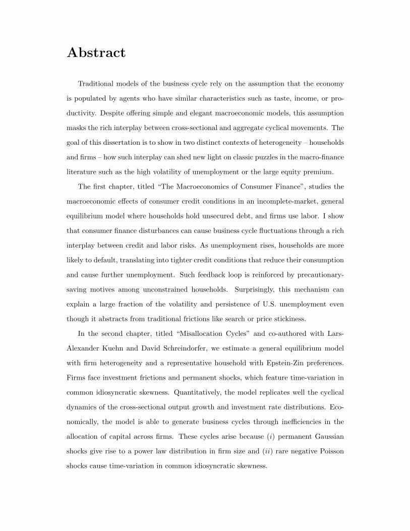
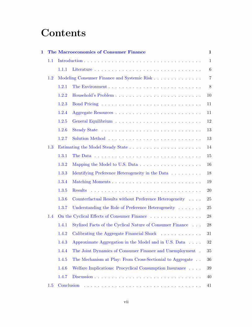
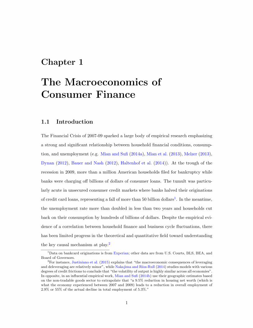
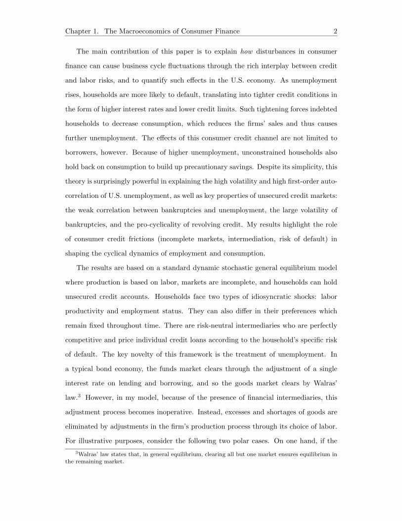