cross-domain matching with squared-loss mutual information · cross-domain matching with...

1IEEE Transactions on Pattern Analysis and Machine Intelligence, vol.37, no.9,pp.1764–1776, 2015.

Cross-Domain Matchingwith Squared-Loss Mutual Information

Makoto YamadaYahoo Labs, USA

[email protected]

Leonid SigalDisney Research Pittsburgh, [email protected]

Michalis RaptisComcast Labs, USA

[email protected]

Machiko ToyodaNTT Labs, Japan

[email protected]

Yi ChangYahoo Labs, USA

[email protected]

Masashi SugiyamaThe University of Tokyo, Japan

[email protected]

Abstract

The goal of cross-domain matching (CDM) is to find correspondences between twosets of objects in different domains in an unsupervised way. CDM has various inter-esting applications, including photo album summarization where photos are auto-matically aligned into a designed frame expressed in the Cartesian coordinate sys-tem, and temporal alignment which aligns sequences such as videos that are poten-tially expressed using different features. In this paper, we propose an information-theoretic CDM framework based on squared-loss mutual information (SMI). Theproposed approach can directly handle non-linearly related objects/sequences withdifferent dimensions, with the ability that hyper-parameters can be objectively op-timized by cross-validation. We apply the proposed method to several real-worldproblems including image matching, unpaired voice conversion, photo album sum-marization, cross-feature video and cross-domain video-to-mocap alignment, andKinect-based action recognition, and experimentally demonstrate that the proposedmethod is a promising alternative to state-of-the-art CDM methods.

Cross-Domain Matching with Squared-Loss Mutual Information 2

Keywords

Cross-Domain Object Matching, Cross-Domain Temporal Alignment, Squared-LossMutual Information.

1 Introduction

Matching/alignment of objects/time-series from different domains is an important task inmachine learning, data mining, and computer vision communities. Applications includephoto album summarization, cross-feature video and cross-domain video-to-mocap align-ment, activity recognition, temporal segmentation, and curve matching [1, 2, 3, 4, 5, 6].In this paper, we propose a general information-theoretic cross-domain matching (CDM)framework based on squared-loss mutual information [7]. In particular, we address twoCDM problems: cross-domain object matching and cross-domain temporal alignment.The difference between the two CDM problems is subtle. In object matching the relativeordering within the sets does not matter, where as in temporal alignment the relativeordering within each set must be preserved.

Cross-Domain Object Matching (CDOM): The objective of cross-domain objectmatching (CDOM) is to match two sets of objects in different domains. For instance,in photo album summarization, photos are automatically assigned into a designed frameexpressed in the Cartesian coordinate system (see Figure 5(a)). A typical approach ofCDOM is to find a mapping from objects in one domain (photos) to objects in the otherdomain (frame) so that the pairwise dependency is maximized. In this scenario, accuratelyevaluating the dependence between objects is the key challenge.

Kernelized sorting (KS) [1] tries to find a mapping between two domains that max-imizes mutual information (MI) [8] under the Gaussian assumption. However, since theGaussian assumption may not be fulfilled in practice, this method (which we refer to asKS-MI) tends to perform poorly. To overcome the limitation of KS-MI, Quadrianto etal. [2] proposed using the kernel-based dependence measure called the Hilbert-Schmidtindependence criterion (HSIC) [9] for KS. Since HSIC is a distribution-free independencemeasure, KS with HSIC (which we refer to as KS-HSIC) is more flexible than KS-MI.However, HSIC includes the Gaussian kernel width as a tuning parameter, and its choiceis crucial in obtaining desired performance (see also [10]).

In this paper, we propose an alternative CDOM method that can naturally addressthe model selection problem. The proposed method, called least-squares object matching(LSOM), employs squared-loss mutual information (SMI) [7] as the dependence measure.An advantage of LSOM is that cross-validation (CV) with respect to the SMI criterionis possible. Thus, all the tuning parameters such as the Gaussian kernel width and theregularization parameter can be objectively determined by CV. Through experiments onimage matching, unpaired voice conversion, and photo album summarization tasks, LSOMis shown to be a promising alternative to CDOM, outperforming competing methods.


Cross-Domain Temporal Alignment (CDTA): Temporal alignment of sequences isan important problem with many practical applications such as speech recognition [11, 12],activity recognition [4], temporal segmentation [5], curve matching [6], chromatographicand micro-array data analysis [13], synthesis of human motion [14], and temporal align-ment of human motion [3, 15].

Dynamic time warping (DTW) is a classical temporal alignment method that alignstwo sequences by minimizing the pairwise distance [11, 12] between samples (e.g., underthe Euclidean, squared Euclidean, or Manhattan distance measures). An advantage ofDTW is that the minimization can be efficiently carried out by dynamic programming(DP). [16]. However, due to the typical fixed sample-wise notion of distance, DTW maynot be able to find a good alignment where two signals are related in complex ways (e.g., avideo and negative of the video are perceptually similar but would result in large sample-to-sample distance and DTW score). Moreover, DTW cannot handle sequences withdifferent dimensions (e.g., video to audio alignment), which limits the range of applicationssignificantly. Even if the dimensionality is the same, it is not clear which distance measureis the most appropriate for a given application.

To overcome the weaknesses of DTW, canonical time warping (CTW) was introducedin [3]. CTW performs sequence alignment in a common latent space found by canonicalcorrelation analysis (CCA) [17]. Thus, CTW can naturally handle sequences with differ-ent dimensions. However, CTW can only deal with linear subspace projections, and it isdifficult to optimize model parameters, such as the regularization parameter used in CCAand the dimensionality of the common latent space. To handle non-linearity, dynamicmanifold temporal warping (DMTW) was recently proposed in [4]. DMTW first projectsoriginal data onto a one-dimensional non-linear manifold and then finds an alignment onthis manifold using DTW. Although DMTW is highly flexible by construction, its perfor-mance depends heavily on the choice of the non-linear transformation and, moreover, itimplicitly assumes the smoothness of sequences.

In this paper, we propose a novel information-theoretic CDTA method based on de-pendence maximization. Our method, which we call least-squares dynamic time warping(LSDTW), employs SMI as a dependency measure. Our method can naturally deal withnon-linearity and non-Gaussianity in data and CV is available for model selection. Fur-thermore, LSDTW does not require strong assumptions on the topology of the latentmanifold (e.g., smoothness). Thus, LSDTW is expected to perform well in a broaderrange of applications. Through experiments on synthetic data, video sequence alignment,and Kinect action recognition tasks, LSDTW is shown to be a promising alternative toexisting temporal alignment methods.

Preliminary version of this work appeared in [18] which only focused on SMI-basedCDOM. In this journal version, we further explore SMI-based CDTA and provide a moreextensive experimental evaluation.


2 Squared-Loss Mutual Information

We first review squared-loss mutual information (SMI) [7].SMI is defined and expressed as

SMI =1

2

∫∫ (p(x,y)

p(x)p(y)− 1

)2

p(x)p(y)dxdy

=1

2

∫∫ (p(x,y)

p(x)p(y)

)p(x,y)dxdy − 1

2. (1)

Note that SMI is the Pearson divergence [19] from p(x,y) to p(x)p(y), while the ordinaryMI is the Kullback-Leibler divergence [20] from p(x,y) to p(x)p(y). SMI is non-negativeand takes zero if and only if x and y are independent, as the ordinary MI.

SMI cannot be directly computed since it contains unknown densities p(x,y), p(x),and p(y). Here, we briefly review an SMI estimation method called least-squares mutualinformation (LSMI) [7].

Suppose that we are given n independent and identically distributed (i.i.d.) pairedsamples {(xi,yi)}ni=1 drawn from a joint distribution with density p(x,y). A key idea ofLSMI is to directly estimate the density ratio,

r(x,y) =p(x,y)

p(x)p(y),

without going through density estimation of p(x,y), p(x), and p(y).In LSMI, the density ratio function r(x,y) is directly modeled by the following linear-

in-parameter model:

rα(x,y) =b∑

ℓ=1

αℓφℓ(x,y) = α⊤φ(x,y), (2)

where b is the number of basis functions, α = (α1, . . . , αb)⊤ are parameters, φ(x,y) =

(φ1(x,y), . . . , φb(x,y))⊤ are basis functions, and ⊤ denotes the transpose. Here, we use

the product kernel of the following form for b = n as basis functions:

φℓ(x,y) = K(x,xℓ)L(y,yℓ),

where K(x,x′) and L(y,y′) are reproducing kernels for x and y. In this paper, we usethe Gaussian kernel.

The parameters α are estimated so that the following squared-error J is minimized:

J(α) =1

2

∫∫(r(x,y)− rα(x,y))

2p(x)p(y)dxdy

= C −∫

rα(x,y)p(x,y)dxdy

+1

2

∫∫rα(x,y)

2p(x)p(y)dxdy,


where we use r(x,y)p(x)p(y) = p(x,y) and C is a constant.By using an empirical approximation, the parameter α in the model rα(x,y) is learned

as follows:

α = argminα

[1

2α⊤Hα− h⊤α+

λ

2α⊤α

], (3)

where a regularization term λα⊤α/2 is included for avoiding overfitting, and

H =1

n2

n∑i,j=1

φ(xi,yj)φ(xi,yj)⊤

=1

n2(KK⊤) ◦ (LL⊤),

h =1

n

n∑i=1

φ(xi,yi)

=1

n(K ◦L)1n,

where ◦ denotes the Hadamard product (a.k.a. the element-wise product) and 1n =[1, . . . , 1]⊤ ∈ Rn.

Differentiating the objective function in Eq.(3) with respect to α and equating it tozero, we can obtain an analytic-form solution:

α = (H + λIb)−1h.

Given a density ratio estimator r = rα, SMI can be simply approximated as

SMI =1

2α⊤h− 1

2. (4)

Model selection: In order to determine the kernel parameter and the regularizationparameter λ, cross-validation (CV) is available for the SMI estimator: First, the samples{(xi,yi)}ni=1 are divided into K disjoint subsets {Sk}Kk=1, Sk = {(xk,i,yk,i)}nk

i=1 of (ap-proximately) the same size, where nk is the number of samples in the subset Sk. Then,an estimator αSk

is obtained using {Sj}j =k, and the approximation error for the hold-outsamples Sk is computed as

J(K-CV)Sk

=1

2α⊤

SkHSk

αSk− h⊤

SkαSk

,

where, for [KSk]ij = K(xi,xk,j), [LSk

]ij = L(yi,yk,j) i = 1, . . . , n, j = 1, . . . , |Sk|,

HSk=

1

n2k

(KSkK⊤

Sk) ◦ (LSk

L⊤Sk),

hSk=

1

nk

(KSk◦LSk

)1nk.


This procedure is repeated for k = 1, . . . , K, and its average J (K-CV) is taken as

J (K-CV) =1

K

K∑k=1

J(K-CV)Sk

.

We compute J (K-CV) for all model candidates, and choose the model that minimizesJ (K-CV).

3 Cross-Domain Object Matching with SMI

In this section, we propose a CDOMmethod called least-squares object matching (LSOM).

3.1 Overview of Least-Squares Object Matching

The goal of CDOM is, given two sets of samples of the same size, {xi}ni=1 and {yi}ni=1, tofind a mapping that well “matches” them. Note that the dimensionality of x and y canbe different.

Let π be a permutation function over {1, . . . , n}, and let Π be the correspondingpermutation indicator matrix, i.e.,

Π ∈ {0, 1}n×n, Π1n = 1n, and Π⊤1n = 1n,

where 1n is the n-dimensional vector with all ones.Let us denote the samples matched by a permutation π by

{(xi,yπ(i))}ni=1.

The optimal permutation, denoted by Π∗, can be obtained as the maximizer of the SMIbetween the two sets X = [x1, . . . ,xn] and Y Π = [yπ(1), . . . ,yπ(n)]:

Π∗ := argmaxΠ

SMI(X,Y Π). (5)

Based on Eq.(5), we develop the following iterative algorithm for optimizing Π:

(i) Initialization: Initialize the alignment matrix Π.

(ii) Dependence estimation: For the current Π, obtain an SMI estimator

SMI(X,Y Π).

(iii) Dependence maximization: Given an SMI estimator SMI(X,Y Π), obtain themaximum alignment Π.

(iv) Convergence check: The above (ii) and (iii) are repeated until Π fulfills a con-vergence criterion.

We call this approach least-squares object matching (LSOM).


3.2 Dependence Estimation

In dependence estimation, we compute Eq.(4) with X and Y Π:

SMI(X,Y Π) =1

2α⊤

ΠhΠ − 1

2, (6)

where

αΠ = (HΠ + λIn)−1hΠ,

HΠ =1

n2(KK⊤) ◦ (Π⊤LL⊤Π),

hΠ =1

n

(K ◦ (Π⊤LΠ)

)1n.

Then, plugging hΠ into Eq.(6), we get

SMI(X,Y Π) =1

2nα⊤

Π

(K ◦ (Π⊤LΠ)

)1n −

1

2

=1

2ntr(Π⊤LΠAΠK

)− 1

2,

where A is the diagonal matrix with diagonal elements given by α. Note that we usedEq.(73) and Eq.(75) in [21] for obtaining the above SMI expression. Note, we use themodel selection presented in Section 2.

3.3 Dependence Maximization

Dependence maximization of LSOM is formulated as follows:

maxΠ

SMI(X,Y Π).

Since this optimization problem is in general NP-hard, we simply use the same optimiza-tion strategy as kernelized sorting [2] (see also Section 5.1.2), i.e., for the current Πold,the solution is updated as

Πnew = (1− η)Πold + η argmaxΠ

tr(Π⊤LΠoldAΠoldK

). (7)

where 0 < η ≤ 1 is a step size. The second term is a linear assignment problem (LAP)[22], which can be efficiently solved by using the Hungarian method [22]. In this paper, aC++ implementation of the Hungarian method provided by Cooper1 was used for solvingEq.(7); then Π is repeatedly updated by Eq.(7) until convergence.

Initialization: In this iterative optimization procedure, the choice of the initial per-mutation matrix is critical to obtain a good solution. Quadrianto et al. [2] proposed a

1http://mit.edu/harold/www/code.html


HSIC-based initialization scheme. HSIC is a kernel-based dependence measure given asfollows [9]:

HSIC(X,Y ) = tr(KL),

where K = ΓKΓ and L = ΓLΓ are the centered kernel matrices for x and y, respectively.Note that smaller HSIC scores mean that X and Y are closer to be independent. In theHSIC-based initialization scheme, the alignment that maximizes HSIC between X and Yis used.

Suppose that the kernel matrices K and L are rank one, i.e., for some f and g, Kand L can be expressed as K = ff⊤ and L = gg⊤. Then HSIC can be written as

HSIC(X,Y Π) = ∥f⊤Πg∥2. (8)

The initial permutation matrix is determined so that Eq.(8) is maximized. Accordingto Theorems 368 and 369 in [23], the maximum of Eq.(8) is attained when the elementsof f and Πg are ordered in the same way. That is, if the elements of f are ordered inthe ascending manner (i.e., f1 ≤ f2 ≤ · · · ≤ fn), the maximum of Eq.(8) is attained byordering the elements of g in the same ascending way. However, since the kernel matricesK and L may not be rank one in practice, the principal eigenvectors of K and L wereused as f and g in [2]. We call this eigenvalue-based initialization.

4 Cross Domain Temporal Alignment via SMI

Next, we propose cross-domain temporal alignment (CDTA) based on SMI [7, 24]. Thekey difference between temporal alignment and object matching is that sample orderingwithin each set must be strictly preserved in temporal alignment, as that accounts for thetemporal order of samples.

4.1 Overview of Least-Squares Dynamic Time Warping (LS-DTW)

Let X = [x1,x2, . . . ,xnx ] and Y = [y1,y2, . . . ,yny ] be sequences, represented by orderedsamples xi ∈ Rdx and yi ∈ Rdy , from different domains. Our goal is to find tempo-ral alignment such that the statistical dependency between two sequences of samples ismaximized. Note that nx and dx can, in general, be different from ny and dy.

Let πx and πy be alignment functions over {1, . . . , nx} and {1, . . . , ny}, and let Π bethe corresponding alignment matrix:

Π := [πx πy]⊤ ∈ R2×m,

πx := [πx1 , . . . , π

xm]

⊤ ∈ {1, . . . , nx}m×1,

πy := [πy1 , . . . , π

ym]

⊤ ∈ {1, . . . , ny}m×1,

where m is the number of indexes needed to align the sequences and ⊤ denotes thetranspose. Π needs to satisfy the following constraints:


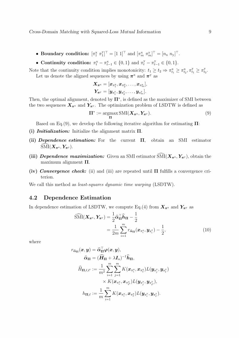
• Boundary condition: [πx1 πy

1 ]⊤ = [1 1]⊤ and [πx

m πym]

⊤ = [nx ny]⊤.

• Continuity condition: πxt − πx

t−1 ∈ {0, 1} and πyt − πy

t−1 ∈ {0, 1}.Note that the continuity condition implies monotonicity: t1 ≥ t2 ⇒ πx

t1≥ πx

t2, πy

t1 ≥ πyt2 .

Let us denote the aligned sequences by using πx and πy as

Xπx = [xπx1,xπx

2, . . . ,xπx

m],

Yπy = [yπy1,yπy

2, . . . ,yπy

m].

Then, the optimal alignment, denoted by Π∗, is defined as the maximizer of SMI betweenthe two sequences Xπx and Yπy . The optimization problem of LSDTW is defined as

Π∗ := argmaxΠ

SMI(Xπx ,Yπy). (9)

Based on Eq.(9), we develop the following iterative algorithm for estimating Π:

(i) Initialization: Initialize the alignment matrix Π.

(ii) Dependence estimation: For the current Π, obtain an SMI estimator

SMI(Xπx ,Yπy).

(iii) Dependence maximization: Given an SMI estimator SMI(Xπx ,Yπy), obtain themaximum alignment Π.

(iv) Convergence check: (ii) and (iii) are repeated until Π fulfills a convergence cri-terion.

We call this method as least-squares dynamic time warping (LSDTW).

4.2 Dependence Estimation

In dependence estimation of LSDTW, we compute Eq.(4) from Xπx and Yπy as

SMI(Xπx ,Yπy) =1

2α⊤

ΠhΠ − 1

2

=1

2m

m∑i=1

rαΠ(xπx

i,yπy

i)− 1

2, (10)

where

rαΠ(x,y) = α⊤

Πφ(x,y),

αΠ = (HΠ + λIn)−1hΠ,

HΠ,ℓ,ℓ′ :=1

m2

m∑i=1

m∑j=1

K(xπxi,xπx

ℓ)L(yπy

j,yπy

ℓ)

×K(xπxi,xπx

ℓ′)L(yπy

j,yπy

ℓ′),

hΠ,ℓ :=1

m

m∑i=1

K(xπxi,xπx

ℓ)L(yπy

i,yπy

ℓ).


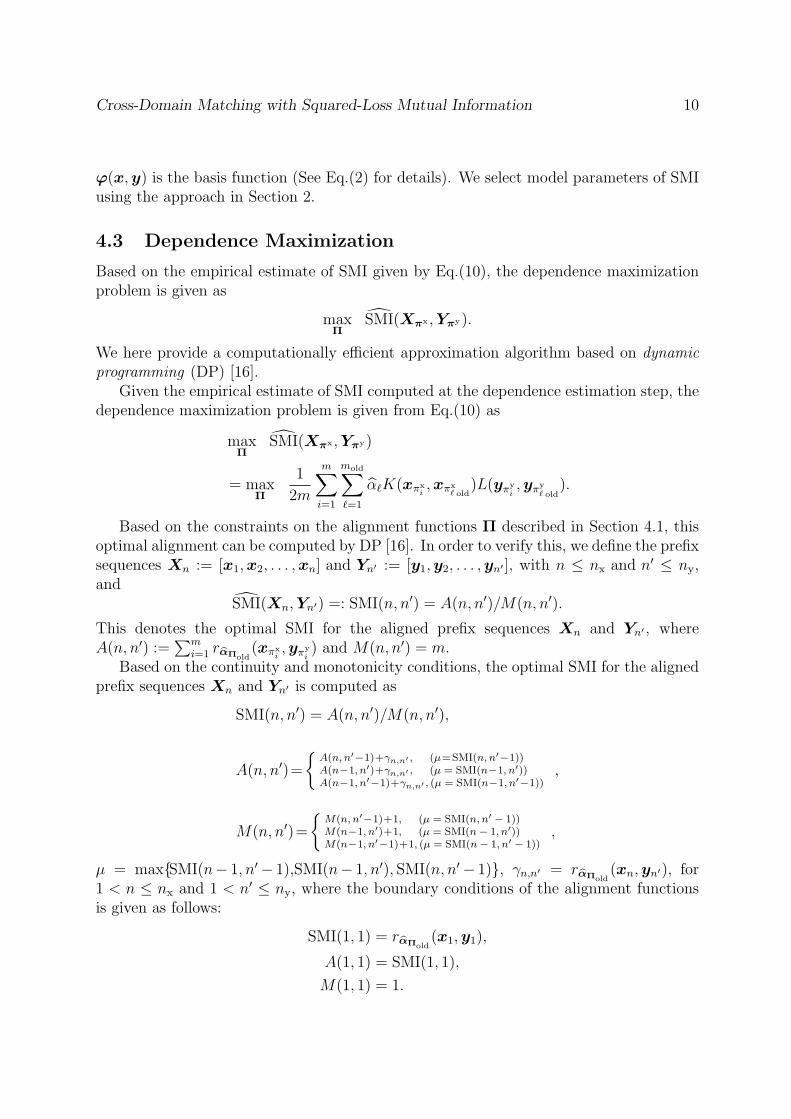
φ(x,y) is the basis function (See Eq.(2) for details). We select model parameters of SMIusing the approach in Section 2.

4.3 Dependence Maximization

Based on the empirical estimate of SMI given by Eq.(10), the dependence maximizationproblem is given as

maxΠ

SMI(Xπx ,Yπy).

We here provide a computationally efficient approximation algorithm based on dynamicprogramming (DP) [16].

Given the empirical estimate of SMI computed at the dependence estimation step, thedependence maximization problem is given from Eq.(10) as

maxΠ

SMI(Xπx ,Yπy)

= maxΠ

1

2m

m∑i=1

mold∑ℓ=1

αℓK(xπxi,xπx

ℓ old)L(yπy

i,yπy

ℓ old).

Based on the constraints on the alignment functions Π described in Section 4.1, thisoptimal alignment can be computed by DP [16]. In order to verify this, we define the prefixsequences Xn := [x1,x2, . . . ,xn] and Yn′ := [y1,y2, . . . ,yn′ ], with n ≤ nx and n′ ≤ ny,and

SMI(Xn,Yn′) =: SMI(n, n′) = A(n, n′)/M(n, n′).

This denotes the optimal SMI for the aligned prefix sequences Xn and Yn′ , whereA(n, n′) :=

∑mi=1 rαΠold

(xπxi,yπy

i) and M(n, n′) = m.

Based on the continuity and monotonicity conditions, the optimal SMI for the alignedprefix sequences Xn and Yn′ is computed as

SMI(n, n′) = A(n, n′)/M(n, n′),

A(n, n′)=

{A(n, n′−1)+γn,n′ , (µ=SMI(n, n′−1))A(n−1, n′)+γn,n′ , (µ = SMI(n−1, n′))A(n−1, n′−1)+γn,n′ , (µ = SMI(n−1, n′−1))

,

M(n, n′)=

{M(n, n′−1)+1, (µ = SMI(n, n′ − 1))M(n−1, n′)+1, (µ = SMI(n− 1, n′))M(n−1, n′−1)+1, (µ = SMI(n− 1, n′ − 1))

,

µ = max{SMI(n− 1, n′− 1),SMI(n− 1, n′), SMI(n, n′− 1)}, γn,n′ = rαΠold(xn,yn′), for

1 < n ≤ nx and 1 < n′ ≤ ny, where the boundary conditions of the alignment functionsis given as follows:

SMI(1, 1) = rαΠold(x1,y1),

A(1, 1) = SMI(1, 1),

M(1, 1) = 1.


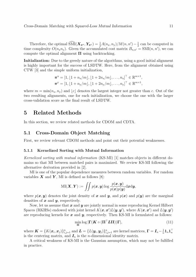
Therefore, the optimal SMI(Xπx ,Yπy) = 12A(nx, ny)/M(n, n′)− 1

2can be computed in

time complexity O(nxny). Given the accumulated cost matrix Bn,n′ = SMI(n, n′), we cancompute the optimal alignment Π using backtracking.

Initialization: Due to the greedy nature of the algorithms, using a good initial alignmentis highly important for the success of LSDTW. Here, from the alignment obtained usingCTW [3] and the simple uniform initialization,

πx = [1, ⌊1 + nx/m⌋, ⌊1 + 2nx/m⌋, . . . , nx]⊤ ∈ Rm×1,

πy = [1, ⌊1 + ny/m⌋, ⌊1 + 2ny/m⌋, . . . , ny]⊤ ∈ Rm×1,

where m = min(nx, ny) and ⌊c⌋ denotes the largest integer not greater than c. Out of thetwo resulting alignments, one for each initialization, we choose the one with the largercross-validation score as the final result of LSDTW.

5 Related Methods

In this section, we review related methods for CDOM and CDTA.

5.1 Cross-Domain Object Matching

First, we review relevant CDOM methods and point out their potential weaknesses.

5.1.1 Kernelized Sorting with Mutual Information

Kernelized sorting with mutual information (KS-MI) [1] matches objects in different do-mains so that MI between matched pairs is maximized. We review KS-MI following thealternative derivation provided in [2].

MI is one of the popular dependence measures between random variables. For randomvariables X and Y , MI is defined as follows [8]:

MI(X,Y ) :=

∫∫p(x,y) log

p(x,y)

p(x)p(y)dxdy,

where p(x,y) denotes the joint density of x and y, and p(x) and p(y) are the marginaldensities of x and y, respectively.

Now, let us assume that x and y are jointly normal in some reproducing Kernel HilbertSpaces (RKHSs) endowed with joint kernel K(x,x′)L(y,y′), where K(x,x′) and L(y,y′)are reproducing kernels for x and y, respectively. Then KS-MI is formulated as follows:

minΠ

log |Γ(K ◦ (Π⊤LΠ))Γ|, (11)

where K = {K(xi,xj)}ni,j=1 and L = {L(yi,yj)}ni,j=1 are kernel matrices, Γ = In− 1n1n1

⊤n

is the centering matrix, and In is the n-dimensional identity matrix.A critical weakness of KS-MI is the Gaussian assumption, which may not be fulfilled

in practice.


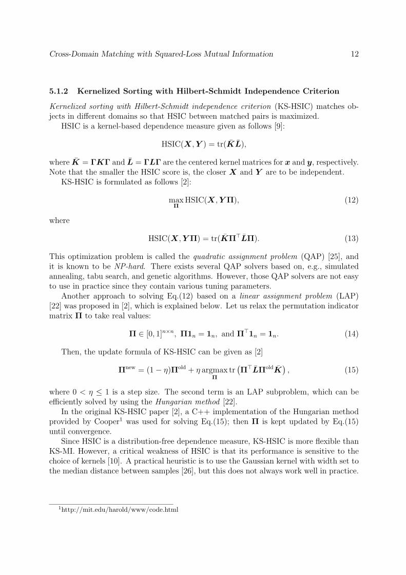
5.1.2 Kernelized Sorting with Hilbert-Schmidt Independence Criterion

Kernelized sorting with Hilbert-Schmidt independence criterion (KS-HSIC) matches ob-jects in different domains so that HSIC between matched pairs is maximized.

HSIC is a kernel-based dependence measure given as follows [9]:

HSIC(X,Y ) = tr(KL),

where K = ΓKΓ and L = ΓLΓ are the centered kernel matrices for x and y, respectively.Note that the smaller the HSIC score is, the closer X and Y are to be independent.

KS-HSIC is formulated as follows [2]:

maxΠ

HSIC(X,Y Π), (12)

where

HSIC(X,Y Π) = tr(KΠ⊤LΠ). (13)

This optimization problem is called the quadratic assignment problem (QAP) [25], andit is known to be NP-hard. There exists several QAP solvers based on, e.g., simulatedannealing, tabu search, and genetic algorithms. However, those QAP solvers are not easyto use in practice since they contain various tuning parameters.

Another approach to solving Eq.(12) based on a linear assignment problem (LAP)[22] was proposed in [2], which is explained below. Let us relax the permutation indicatormatrix Π to take real values:

Π ∈ [0, 1]n×n, Π1n = 1n, and Π⊤1n = 1n. (14)

Then, the update formula of KS-HSIC can be given as [2]


tr(Π⊤LΠoldK

), (15)

where 0 < η ≤ 1 is a step size. The second term is an LAP subproblem, which can beefficiently solved by using the Hungarian method [22].

In the original KS-HSIC paper [2], a C++ implementation of the Hungarian methodprovided by Cooper1 was used for solving Eq.(15); then Π is kept updated by Eq.(15)until convergence.

Since HSIC is a distribution-free dependence measure, KS-HSIC is more flexible thanKS-MI. However, a critical weakness of HSIC is that its performance is sensitive to thechoice of kernels [10]. A practical heuristic is to use the Gaussian kernel with width set tothe median distance between samples [26], but this does not always work well in practice.

1http://mit.edu/harold/www/code.html


5.1.3 Kernelized Sorting with Normalized Cross-Covariance Operator

The kernel-based dependence measure based on the normalized cross-covariance operator(NOCCO) [27] is given as follows [27]:

DNOCCO(Z) = tr(KL),

where K = K(K+nϵIn)−1, L = L(L+nϵIn)

−1, and ϵ > 0 is a regularization parameter.DNOCCO was shown to be asymptotically independent of the choice of kernels. Thus, KSwith DNOCCO (KS-NOCCO) is expected to be less sensitive to the kernel parameter choicethan KS-HSIC [18].

The dependency measure for Z(Π) can be written as [18]

DNOCCO(Z(Π)) = tr(KΠ⊤LΠ).

Since this is essentially the same form as HSIC, a local optimal solution may beobtained in the same way as KS-HSIC:


tr(Π⊤LΠoldK

). (16)

However, the property that DNOCCO is independent of the kernel choice holds only asymp-totically. Thus, with finite samples, DNOCCO does still depend on the choice of kernels aswell as the regularization parameter ϵ which needs to be manually tuned.

5.2 Cross-Domain Temporal Alignment

Next, we review relevant temporal alignment methods which are based on pairwise dis-tance minimization (not dependence maximization) and point out their potential weak-nesses.

5.2.1 Dynamic Time Warping (DTW)

The goal of dynamic time warping (DTW) is, given two sequences of the same dimension-ality with different lengths, X and Y , to find an alignment such that the sum of pairwisedistances between two sequences is minimized [11, 12]:

minWx,Wy

∥XW⊤x − Y W⊤

y ∥2Frob,

where ∥ · ∥Frob is the Frobenius norm, Wx ∈ {0, 1}m×nx and Wy ∈ {0, 1}m×ny are binaryselection matrices that need to be estimated to align X and Y . The above DTW opti-mization problem can be efficiently solved by DP with time complexity O(nxny). However,DTW tends to fail if the magnitude of two sequences are different. To deal with this issue,the Derivative dynamic time warping (DDTW) [28], which aligns the first order derivativeof sequences, is useful.


Potential weaknesses of DTW and DDTW are that they cannot handle sequenceswith different dimensionalities such as image-to-audio alignment. Moreover, even whenthe dimensionality of the sequences is the same, DTW and DDTW may not be able tofind a good alignment of sequences with different characteristics such as sequences withdifferent amplitudes. These drawbacks highly limit the applicability of DTW and DDTW.

5.2.2 Iterative Motion Warping (IMW)

The optimization problem of the iterative motion warping (IWM) [29] is given as

minA,B,W

∥(X ◦Ax +Bx)W⊤x − (Y ◦Ay +By)W

⊤y ∥2Frob

+R(Ax,Ay,Bx,By),

where Ax ∈ Rd×nx and Ay ∈ Rd×ny are the scaling matrices, Bx ∈ Rd×nx and By ∈Rd×nx are the translation matrices, ◦ is the Hadamard product, R(Ax,Ay,Bx,By) is theregularization term to avoid overfitting.

IMW can successfully deal with sequences with different characteristics, e.g., hav-ing different amplitudes. However, similarly to the original DTW, IMW cannot handlesequences with different dimensionalities.

5.2.3 Canonical Time Warping (CTW)

Canonical time warping (CTW) can align sequences with different dimensionalities byconsidering a common latent space [3, 15].

The CTW optimization problem is given as

minWx,Wy,Vx,Vy

∥V ⊤x XW⊤

x − V ⊤y Y W⊤

y ∥2Frob, (17)

where Vx ∈ Rdx×b and Vy ∈ Rdy×b (b ≤ min(dx, dy)) are linear projection matrices of xand y onto a common latent space, respectively. The above optimization problem can beefficiently solved by alternately performing CCA and DTW, where the alignment matrixobtained using DTW is usually used as an initial alignment matrix.

Generalized time warping (GTW) [15] can be regarded as CTW if we align two se-quences and use the dynamic programming to obtain an alignment.

A limitation of CTW is that, since CTW finds a common latent space using CCA,it can only deal with linear and Gaussian temporal alignment problems. Thus, CTWcannot properly deal with multi-modal and non-Gaussian data. Another limitation ofCTW is that comparing the alignment quality over different model parameters is notstraightforward. This is because, for different model parameters, common latent spacesfound by CCA are generally different and thus the metrics of the pairwise distance (17) arealso different. For this reason, a systematic model selection method for the regularizationparameter, the dimensionality of the common latent space, and the initial alignmentmatrix has not been properly addressed so far, to the best of our knowledge.


5.2.4 Kernelized Canonical Time Warping (KCTW)

Let us transform X and Y to higher dimensional matrices Φ and Ψ and define Vx = ΦVx

and Vy = ΨVy. Then, we have a nonlinear version of CTW (Eq.(17)) as

minWx,Wy,Vx,Vy

∥V ⊤x KxW

⊤x − V ⊤

y KyW⊤y ∥2Frob, (18)

where Kx = Φ⊤Φ and Ky = Ψ⊤Ψ are the Gram matrices.Using this formulation, one can handle nonlinearity in the CTW framework. However,

it is not clear how to objectively select model parameters such as kernel parameters. Thatis, the KCCA-based approach works well only when appropriate model parameters areused. However, if the parameters are not chosen carefully, KCTW can perform poorly.

6 Experiments

In this section, we report experimental results.

6.1 Cross-Domain Object Matching

First, we experimentally evaluate the performance of our proposed CDOM method inimage matching, unpaired voice conversion, and photo album summarization.

6.1.1 Setup

In all the methods, we use the Gaussian kernels:

K(x,x′) = exp

(−∥x− x′∥2

2σ2x

),

L(y,y′) = exp

(−∥y − y′∥2

2σ2y

),

and we experimentally set the maximum number of iterations for updating permutationmatrices to 20 and the step size η to 1. To avoid falling into undesirable local optima,optimization is carried out 10 times with different initial permutation matrices, which aredetermined by the eigenvalue-based initialization heuristic with Gaussian kernel widths

(σx, σy) = c× (mx,my),

where c = 11/2, 21/2, . . . , 101/2, and

mx = 2−1/2median({∥xi − xj∥}ni,j=1),

my = 2−1/2median({∥yi − yj∥}ni,j=1).


In KS-HSIC and KS-NOCCO, we use the Gaussian kernel with the following widths:

(σx, σy) = c′ × (mx,my),

where c′ = 11/2, 101/2. In KS-NOCCO, we use the following regularization parameters:

ϵ = 0.01, 0.05.

In KS-HSIC (CV), we choose the model parameters of HSIC, σx and σy by 2-fold CVfrom


where we use the cross-validation approach proposed in [30].In LSOM, we choose the model parameters of LSMI, σx, σy, and λ by 2-fold CV1 from


λ = 10−1, 10−2, 10−3.

6.1.2 Image Matching

Let us consider a toy image matching problem. In this experiment, we use images with theRGB format used in [2], which were originally extracted from Flickr 2. We first convertthe images from the RGB space to the Lab space and resize them to 40 × 40 pixels.Then, we vertically divide the images in the middle, and make two sets of half-imagesof 40 × 20 pixels. We denote the vectorized images by {xi}ni=1 and {yi}ni=1, which are2400-dimensional vectors (2400 = 40 × 20 × 3). We then decouple them by randomlypermuting {yi}ni=1, and try to recover the correct correspondence by a CDOM method.

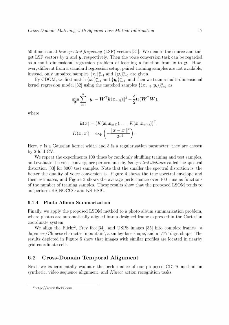
Figure 1 summarizes the average correct matching rate over 100 runs as functions ofthe number of images, showing that the proposed LSOM method tends to outperformthe optimally tuned KS-HSIC, KS-HSIC (CV), and KS-NOCCO methods. Moreover,through experiments, we observed that the optimally tuned KS-HSIC compares favorablywith KS-HSIC (CV). Figure 2 depicts an example of image matching results obtained byLSOM, showing that most of the images are correctly matched. Moreover, we plot thelearning curve of LSOM in Figure 1(c) and it converges in 10 steps. Note that the tuningparameters of LSOM (σx, σy, and λ) are automatically tuned by CV.

6.1.3 Unpaired Voice Conversion

Next, we consider an unpaired voice conversion task, which is aimed at matching the voiceof a source speaker with that of a target speaker.

In this experiment, we use 200 short utterance samples recorded from two male speak-ers in French, with sampling rate 44.1kHz. We first convert the utterance samples to

1We choose 2-fold cross validation to reduce the computational cost.2http://www.flickr.com


50-dimensional line spectral frequency (LSF) vectors [31]. We denote the source and tar-get LSF vectors by x and y, respectively. Then the voice conversion task can be regardedas a multi-dimensional regression problem of learning a function from x to y. How-ever, different from a standard regression setup, paired training samples are not available;instead, only unpaired samples {xi}ni=1 and {yi}ni=1 are given.

By CDOM, we first match {xi}ni=1 and {yi}ni=1, and then we train a multi-dimensionalkernel regression model [32] using the matched samples {(xπ(i),yi)}ni=1 as

minW

n∑i=1

∥yi −W⊤k(xπ(i))∥2 +δ

2tr(W⊤W ),

where

k(x) = (K(x,xπ(1)), . . . , K(x,xπ(n)))⊤,

K(x,x′) = exp

(−∥x− x′∥2

2τ 2

).

Here, τ is a Gaussian kernel width and δ is a regularization parameter; they are chosenby 2-fold CV.

We repeat the experiments 100 times by randomly shuffling training and test samples,and evaluate the voice convergence performance by log-spectral distance called the spectraldistortion [33] for 8000 test samples. Note that the smaller the spectral distortion is, thebetter the quality of voice conversion is. Figure 4 shows the true spectral envelope andtheir estimates, and Figure 3 shows the average performance over 100 runs as functionsof the number of training samples. These results show that the proposed LSOM tends tooutperform KS-NOCCO and KS-HSIC.

6.1.4 Photo Album Summarization

Finally, we apply the proposed LSOM method to a photo album summarization problem,where photos are automatically aligned into a designed frame expressed in the Cartesiancoordinate system.

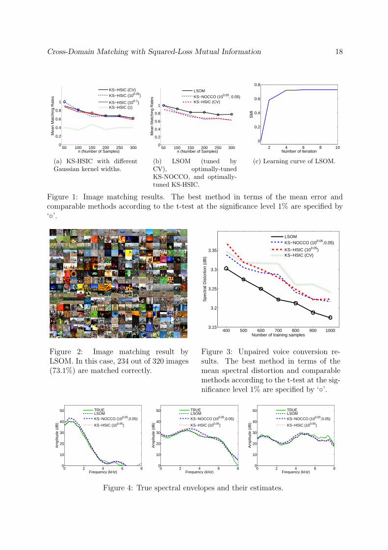
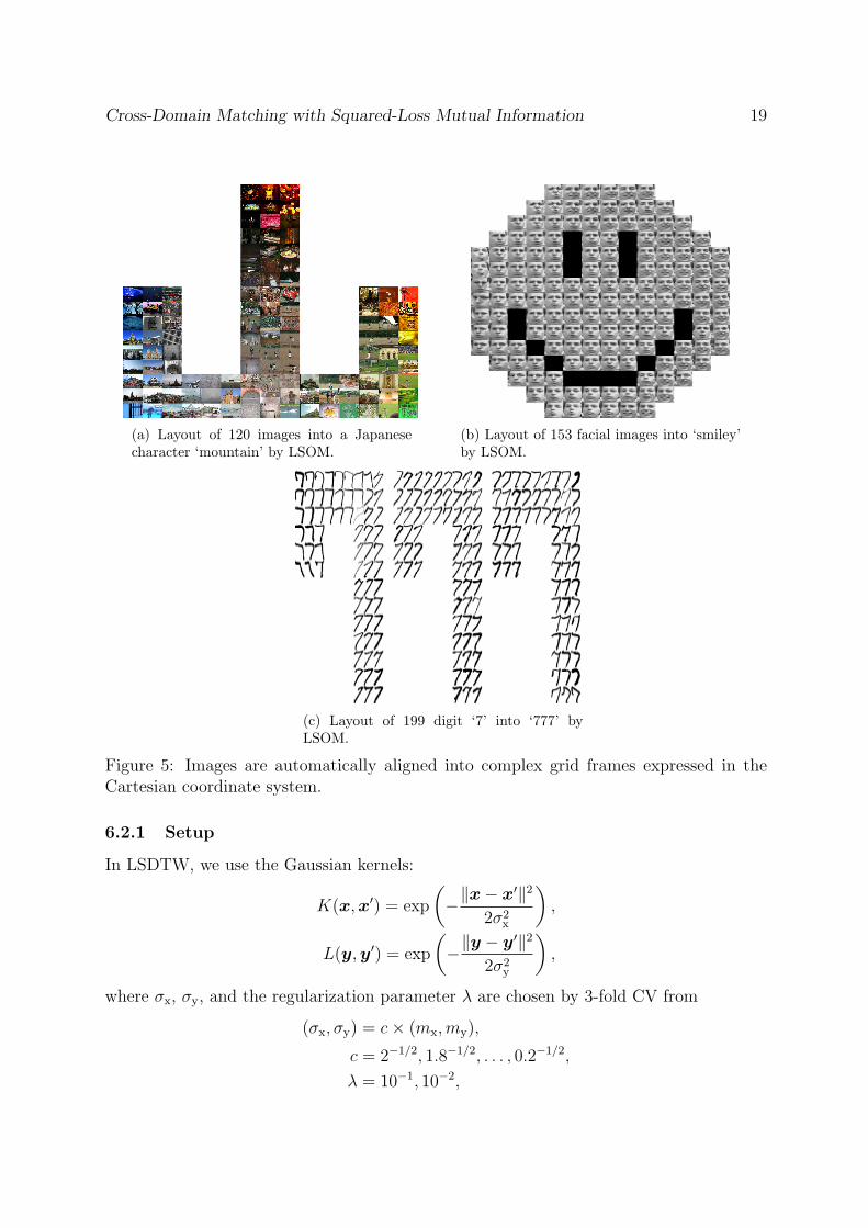
We align the Flickr2, Frey face[34], and USPS images [35] into complex frames—aJapanese/Chinese character ‘mountain’, a smiley-face shape, and a ‘777’ digit shape. Theresults depicted in Figure 5 show that images with similar profiles are located in nearbygrid-coordinate cells.

6.2 Cross-Domain Temporal Alignment

Next, we experimentally evaluate the performance of our proposed CDTA method onsynthetic, video sequence alignment, and Kinect action recognition tasks.

2http://www.flickr.com


50 100 150 200 250 3000

0.2

0.4

0.6

0.8

1

n (Number of Samples)

Mea

n M

atch

ing

Rat

es

KS−HSIC (CV)KS−HSIC (100.05)

KS−HSIC (100.1)KS−HSIC (1)

(a) KS-HSIC with differentGaussian kernel widths.

50 100 150 200 250 3000

0.2

0.4

0.6

0.8

1

n (Number of Samples)M

ean

Mat

chin

g R

ates

LSOM

KS−NOCCO (100.05, 0.05)KS−HSIC (CV)

(b) LSOM (tuned byCV), optimally-tunedKS-NOCCO, and optimally-tuned KS-HSIC.

2 4 6 8 10

0

0.2

0.4

0.6

0.8

Number of iteration

SM

I

(c) Learning curve of LSOM.

Figure 1: Image matching results. The best method in terms of the mean error andcomparable methods according to the t-test at the significance level 1% are specified by‘◦’.

Figure 2: Image matching result byLSOM. In this case, 234 out of 320 images(73.1%) are matched correctly.

400 500 600 700 800 900 10003.15

3.2

3.25

3.3

3.35

Number of training samples

Spe

ctra

l Dis

tort

ion

(dB

)

LSOMKS−NOCCO (100.05,0.05)

KS−HSIC (100.05)KS−HSIC (CV)

Figure 3: Unpaired voice conversion re-sults. The best method in terms of themean spectral distortion and comparablemethods according to the t-test at the sig-nificance level 1% are specified by ‘◦’.

0 2 4 6 80

10

20

30

40

50

Frequency (kHz)

Am

plitu

de (

dB)

TRUELSOMKS−NOCCO (100.05,0.05)

KS−HSIC (100.05)

0 2 4 6 80

10

20

30

40

50

Frequency (kHz)

Am

plitu

de (

dB)


KS−HSIC (100.05)

0 2 4 6 80

10

20

30

40

50

Frequency (kHz)

Am

plitu

de (

dB)


KS−HSIC (100.05)

Figure 4: True spectral envelopes and their estimates.


(a) Layout of 120 images into a Japanesecharacter ‘mountain’ by LSOM.

(b) Layout of 153 facial images into ‘smiley’by LSOM.

(c) Layout of 199 digit ‘7’ into ‘777’ byLSOM.

Figure 5: Images are automatically aligned into complex grid frames expressed in theCartesian coordinate system.

6.2.1 Setup

In LSDTW, we use the Gaussian kernels:

K(x,x′) = exp

(−∥x− x′∥2

2σ2x

),

L(y,y′) = exp

(−∥y − y′∥2

2σ2y

),

where σx, σy, and the regularization parameter λ are chosen by 3-fold CV from


c = 2−1/2, 1.8−1/2, . . . , 0.2−1/2,

λ = 10−1, 10−2,


and

mx = 2−1/2median({∥xi − xj∥}nxi,j=1),

my = 2−1/2median({∥yi − yj∥}ny

i,j=1).

Comparisons: We compare the performance of LSDTWwith DTW and CTW. For DTWand CTW, we use the publicly available implementations provided by the authors of theoriginal papers [3, 15]2. For CTW, we choose the dimensionality of CCA to preserve90% of the total correlation, and we fix the regularization parameter at 0.01. We usethe alignment given by DTW as the initial alignment for CTW. In the video sequencealignment and the real-world Kinect action recognition experiments, we also compareLSDTW to kernel CTW (KCTW), derivative DTW (DDTW) [28], and iterative motionwarping (IMW) [29]. In KCTW, we use the Gaussian kernel and set the kernel width atmx and my, which is a common heuristic [32]. For existing methods, we use the sameparameters as those used in [15].

Evaluation: To evaluate the alignment results, we use the following standard alignmenterror [15]:

Error =dist(Π∗, Π) + dist(Π,Π∗)

m∗ + m,

where

dist(Π1,Π2) =

m1∑i=1

min({∥π(i)1 − π

(j)2 ∥}m2

j=1),

Π∗ and Π are true and estimated alignment matrices, and π(i)1 ,π

(j)2 ∈ R2×1 are the i-th

and j-th columns of Π1 and Π2, respectively.

6.2.2 Synthetic Dataset

We first illustrate the behavior of the proposed LSDTW method on aligning two non-linearly related non-stationary sequences using a synthetic dataset.

We use the following function:

xi = i/200 + 0.4 sin(πi/100) + ei, i = 1, . . . , 200,

yj = ((j − 1)× 2 + 1)/200 + ej, j = 1, . . . , 100,

where ei and ej are randomly generated additive Gaussian noise with standard deviation0.01 (see Figure 6(a) and (b)). Note that, sample-wise, for a given value of xi there maybe multiple yj’s.

2www.f-zhou.com/ta_code.html.


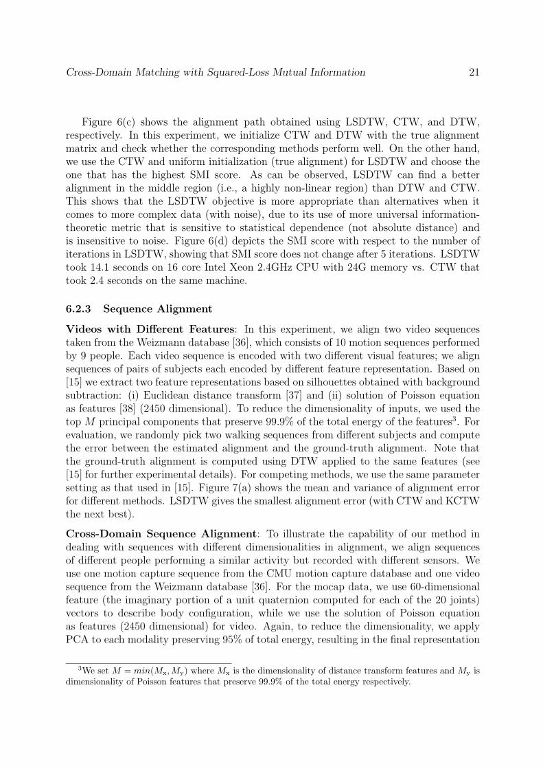
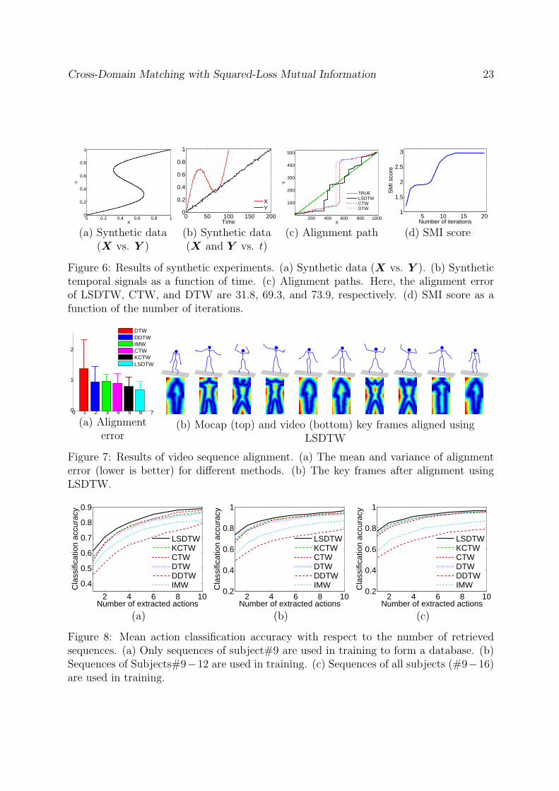
Figure 6(c) shows the alignment path obtained using LSDTW, CTW, and DTW,respectively. In this experiment, we initialize CTW and DTW with the true alignmentmatrix and check whether the corresponding methods perform well. On the other hand,we use the CTW and uniform initialization (true alignment) for LSDTW and choose theone that has the highest SMI score. As can be observed, LSDTW can find a betteralignment in the middle region (i.e., a highly non-linear region) than DTW and CTW.This shows that the LSDTW objective is more appropriate than alternatives when itcomes to more complex data (with noise), due to its use of more universal information-theoretic metric that is sensitive to statistical dependence (not absolute distance) andis insensitive to noise. Figure 6(d) depicts the SMI score with respect to the number ofiterations in LSDTW, showing that SMI score does not change after 5 iterations. LSDTWtook 14.1 seconds on 16 core Intel Xeon 2.4GHz CPU with 24G memory vs. CTW thattook 2.4 seconds on the same machine.

6.2.3 Sequence Alignment

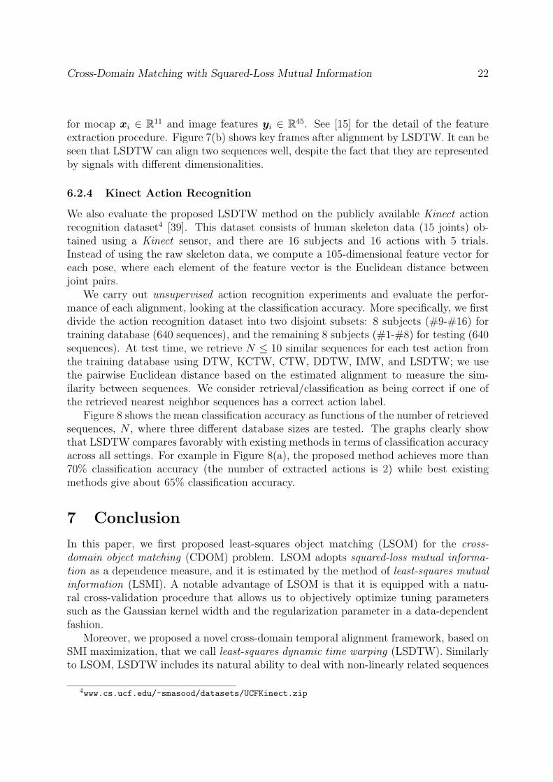
Videos with Different Features: In this experiment, we align two video sequencestaken from the Weizmann database [36], which consists of 10 motion sequences performedby 9 people. Each video sequence is encoded with two different visual features; we alignsequences of pairs of subjects each encoded by different feature representation. Based on[15] we extract two feature representations based on silhouettes obtained with backgroundsubtraction: (i) Euclidean distance transform [37] and (ii) solution of Poisson equationas features [38] (2450 dimensional). To reduce the dimensionality of inputs, we used thetop M principal components that preserve 99.9% of the total energy of the features3. Forevaluation, we randomly pick two walking sequences from different subjects and computethe error between the estimated alignment and the ground-truth alignment. Note thatthe ground-truth alignment is computed using DTW applied to the same features (see[15] for further experimental details). For competing methods, we use the same parametersetting as that used in [15]. Figure 7(a) shows the mean and variance of alignment errorfor different methods. LSDTW gives the smallest alignment error (with CTW and KCTWthe next best).

Cross-Domain Sequence Alignment: To illustrate the capability of our method indealing with sequences with different dimensionalities in alignment, we align sequencesof different people performing a similar activity but recorded with different sensors. Weuse one motion capture sequence from the CMU motion capture database and one videosequence from the Weizmann database [36]. For the mocap data, we use 60-dimensionalfeature (the imaginary portion of a unit quaternion computed for each of the 20 joints)vectors to describe body configuration, while we use the solution of Poisson equationas features (2450 dimensional) for video. Again, to reduce the dimensionality, we applyPCA to each modality preserving 95% of total energy, resulting in the final representation

3We set M = min(Mx,My) where Mx is the dimensionality of distance transform features and My isdimensionality of Poisson features that preserve 99.9% of the total energy respectively.


for mocap xi ∈ R11 and image features yi ∈ R45. See [15] for the detail of the featureextraction procedure. Figure 7(b) shows key frames after alignment by LSDTW. It can beseen that LSDTW can align two sequences well, despite the fact that they are representedby signals with different dimensionalities.

6.2.4 Kinect Action Recognition

We also evaluate the proposed LSDTW method on the publicly available Kinect actionrecognition dataset4 [39]. This dataset consists of human skeleton data (15 joints) ob-tained using a Kinect sensor, and there are 16 subjects and 16 actions with 5 trials.Instead of using the raw skeleton data, we compute a 105-dimensional feature vector foreach pose, where each element of the feature vector is the Euclidean distance betweenjoint pairs.

We carry out unsupervised action recognition experiments and evaluate the perfor-mance of each alignment, looking at the classification accuracy. More specifically, we firstdivide the action recognition dataset into two disjoint subsets: 8 subjects (#9-#16) fortraining database (640 sequences), and the remaining 8 subjects (#1-#8) for testing (640sequences). At test time, we retrieve N ≤ 10 similar sequences for each test action fromthe training database using DTW, KCTW, CTW, DDTW, IMW, and LSDTW; we usethe pairwise Euclidean distance based on the estimated alignment to measure the sim-ilarity between sequences. We consider retrieval/classification as being correct if one ofthe retrieved nearest neighbor sequences has a correct action label.

Figure 8 shows the mean classification accuracy as functions of the number of retrievedsequences, N , where three different database sizes are tested. The graphs clearly showthat LSDTW compares favorably with existing methods in terms of classification accuracyacross all settings. For example in Figure 8(a), the proposed method achieves more than70% classification accuracy (the number of extracted actions is 2) while best existingmethods give about 65% classification accuracy.

7 Conclusion

In this paper, we first proposed least-squares object matching (LSOM) for the cross-domain object matching (CDOM) problem. LSOM adopts squared-loss mutual informa-tion as a dependence measure, and it is estimated by the method of least-squares mutualinformation (LSMI). A notable advantage of LSOM is that it is equipped with a natu-ral cross-validation procedure that allows us to objectively optimize tuning parameterssuch as the Gaussian kernel width and the regularization parameter in a data-dependentfashion.

Moreover, we proposed a novel cross-domain temporal alignment framework, based onSMI maximization, that we call least-squares dynamic time warping (LSDTW). Similarlyto LSOM, LSDTW includes its natural ability to deal with non-linearly related sequences

4www.cs.ucf.edu/~smasood/datasets/UCFKinect.zip


0 0.2 0.4 0.6 0.8 10

0.2

0.4

0.6

0.8

1

X

Y

(a) Synthetic data(X vs. Y )

0 50 100 150 2000

0.2

0.4

0.6

0.8

1

Time

XY

(b) Synthetic data(X and Y vs. t)

200 400 600 800 1000

100

200

300

400

500

X

Y

TRUELSDTWCTWDTW

(c) Alignment path

5 10 15 201

1.5

2

2.5

3

Number of iterations

SM

I sco

re

(d) SMI score

Figure 6: Results of synthetic experiments. (a) Synthetic data (X vs. Y ). (b) Synthetictemporal signals as a function of time. (c) Alignment paths. Here, the alignment errorof LSDTW, CTW, and DTW are 31.8, 69.3, and 73.9, respectively. (d) SMI score as afunction of the number of iterations.

0 1 2 3 4 5 6 70

1

2

DTWDDTWIMWCTWKCTWLSDTW

(a) Alignmenterror

(b) Mocap (top) and video (bottom) key frames aligned usingLSDTW

Figure 7: Results of video sequence alignment. (a) The mean and variance of alignmenterror (lower is better) for different methods. (b) The key frames after alignment usingLSDTW.

2 4 6 8 10

0.4

0.5

0.6

0.7

0.8

0.9

Number of extracted actions

Cla

ssifi

catio

n ac

cura

cy

LSDTWKCTWCTWDTWDDTWIMW

(a)

2 4 6 8 100.2

0.4

0.6

0.8

1


Cla

ssifi

catio

n ac

cura

cy


(b)

2 4 6 8 100.2

0.4

0.6

0.8

1


Cla

ssifi

catio

n ac

cura

cy


(c)

Figure 8: Mean action classification accuracy with respect to the number of retrievedsequences. (a) Only sequences of subject#9 are used in training to form a database. (b)Sequences of Subjects#9−12 are used in training. (c) Sequences of all subjects (#9−16)are used in training.


with different dimensionalities (with non-Gaussian noise) and its ability to optimize modelparameters, such as the Gaussian kernel width and the regularization parameter, by cross-validation.

We applied the proposed methods to various problems including image matching,unpaired voice conversion, photo album summarization, cross-feature video alignment,cross-domain video-to-mocap alignment, and Kinect action recognition, and quantita-tively showed that LSOM and LSDTW are promising alternatives to state-of-the-artcross-domain matching methods.

There are several remaining issues that we leave for future work. For example, match-ing/alignment of multiple objects/sequences, similar to [15], can be addressed by com-puting squared-loss mutual information for more than two variables [40]. Moreover, onecan integrate dimensionality reduction into SMI estimation [41], potentially further im-proving the temporal alignment performance. Finally, CDOM methods cannot handlethe matching problem more than 10K samples. Recently, several efficient graph match-ing algorithms including a path following algorithm [42] and deformable graph matching[43] are proposed. Thus, scaling up the KS and LSOM using the state-of-the-art graphmatching algorithms is also an interesting problem.

Acknowledgments

We thank Dr. Fernando Villavicencio and Dr. Akisato Kimura for their valuable com-ments. We also thank Dr. Feng Zhou and Dr. Fernando de la Torre for data and valuablediscussions. Makoto Yamada was supported by the JST PRESTO program, and MasashiSugiyama was supported by AOARD and KAKENHI 25700022.

References

[1] T. Jebara, “Kernelized sorting, permutation, and alignment for minimum volumePCA,” in Conference on Computational Learning theory (COLT), 2004, pp. 609–623.

[2] N. Quadrianto, A. Smola, L. Song, and T. Tuytelaars, “Kernelized sorting,” IEEETransactions on Pattern Analysis and Machine Intelligence, vol. 32, pp. 1809–1821,October 2010.

[3] F. Zhou and F. De la Torre, “Canonical time warping for alignment of human behav-ior,” in Advances in Neural Information Processing Systems 22, 2009, pp. 2286–2294.

[4] D. Gong and G. G. Medioni, “Dynamic manifold warping for view invariant actionrecognition,” in ICCV, 2011.

[5] F. Zhou, F. De la Torre, and J. K. Hodgins, “Aligned cluster analysis for temporalsegmentation of human motion,” in Automatic Face & Gesture Recognition (FG),2008, pp. 1–7.


[6] T. B. Sebastian, P. N. Klein, and B. B. Kimia, “B.b.: On aligning curves,” IEEETPAMI, pp. 116–124, 2003.

[7] T. Suzuki, M. Sugiyama, T. Kanamori, and J. Sese, “Mutual information estimationreveals global associations between stimuli and biological processes,” BMC Bioinfor-matics, vol. 10, no. S52, 2009.

[8] T. M. Cover and J. A. Thomas, Elements of Information Theory, 2nd ed. Hoboken,NJ, USA: John Wiley & Sons, Inc., 2006.

[9] A. Gretton, O. Bousquet, A. Smola, and B. Scholkopf, “Measuring statistical depen-dence with Hilbert-Schmidt norms,” in 16th International Conference on AlgorithmicLearning Theory (ALT 2005), 2005, pp. 63–78.

[10] J. Jagarlamudi, S. Juarez, and H. Daume III, “Kernelized sorting for natural languageprocessing,” in Proceedings of the Twenty-Fourth AAAI Conference on Artificial In-telligence (AAAI2010), Atlanta, Georgia, U.S.A, Jul. 11-15 2010, pp. 1020–1025.

[11] H. Sakoe and S. Chiba, “Dynamic programming algorithm optimization for spokenword recognition,” IEEE Transactions on Acoustics, Speech, and Signal Processing,no. 1, pp. 43–49, 1978.

[12] L. Rabiner and B. Juang, Fundamentals of Speech Recognition. Prentice-Hall SignalProcessing Series, 1993.

[13] J. Listgarten, R. M. Neal, S. T. Roweis, and A. Emili, “Multiple alignment of con-tinuous time series,” in Advances in neural information processing systems 18, 2005,pp. 817–824.

[14] E. Hsu, K. Pulli, and J. Popovi, “Style translation for human motion,” ACM Trans-actions on Graphics, vol. 24, pp. 1082–1089, 2005.

[15] F. Zhou and F. De la Torre, “Generalized time warping for multi-modal alignmentof human motion,” in CVPR, 2012, pp. 1282–1289.

[16] R. Bellman, “On the Theory of Dynamic Programming,” in Proceedings of the Na-tional Academy of Sciences, vol. 38, 1952, pp. 716–719.

[17] H. Hotelling, “Relations Between Two Sets of Variates,” Biometrika, vol. 28, no. 3/4,pp. 321–377, 1936.

[18] M. Yamada and M. Sugiyama, “Cross-domain object matching with model selection,”AISTATS, pp. 807–815, 2011.

[19] K. Pearson, “On the criterion that a given system of deviations from the probable inthe case of a correlated system of variables is such that it can be reasonably supposedto have arisen from random sampling,” Philosophical Magazine, vol. 50, pp. 157–175,1900.


[20] S. Kullback and R. A. Leibler, “On information and sufficiency,” Annals of Mathe-matical Statistics, vol. 22, pp. 79–86, 1951.

[21] T. P. Minka, “Old and new matrix algebra useful for statistics,” MIT Media Lab,Tech. Rep., 2000.

[22] H. Kuhn, “The Hungarian method for the assignment problem,” Naval ResearchLogistics Quarterly, vol. 2, no. 1-2, pp. 83–97, 1955.

[23] G. H. Hardy, J. E. Littlewood, and G. Polya, Inequalities. Cambridge: CambridgeUniversity Press, 1952.

[24] M. Sugiyama, “Machine learning with squared-loss mutual information,” Entropy,vol. 15, no. 1, pp. 80–112, 2013.

[25] G. Finke, R. E. Burkard, and F. Rendl, “Quadratic assignment problems,” Annalsof Discrete Mathematics, vol. 31, pp. 61–82, 1987.

[26] K. Fukumizu, F. R. Bach, and M. Jordan, “Kernel dimension reduction in regression,”The Annals of Statistics, vol. 37, no. 4, pp. 1871–1905, 2009.

[27] K. Fukumizu, A. Gretton, X. Sun, and B. Scholkopf, “Kernel measures of conditionaldependence,” in Advances in Neural Information Processing Systems 21, D. Koller,D. Schuurmans, Y. Bengio, and L. Botton, Eds. Cambridge, MA: MIT Press, 2009,pp. 489–496.

[28] E. J. Keogh and M. J. Pazzani, “Derivative dynamic time warping,” in SDM, 2001.

[29] E. Hsu, K. Pulli, and J. Popovic, “Style translation for human motion,” ACM Trans-actions on Graphics (TOG), vol. 24, no. 3, pp. 1082–1089, 2005.

[30] M. Sugiyama and M. Yamada, “On kernel parameter selection in hilbert-schmidtindependence criterion,” IEICE TRANSACTIONS on Information and Systems,vol. 95, no. 10, pp. 2564–2567, 2012.

[31] A. Kain and M. W. Macon, “Spectral voice conversion for text-to-speech synthesis,”in Proceedings of 1998 IEEE International Conference on Acoustics, Speech, andSignal Processing (ICASSP1998), Washington, DC, U.S.A, May. 12–15 1988, pp.285–288.

[32] B. Scholkopf and A. J. Smola, Learning with Kernels. Cambridge, MA: MIT Press,2002.

[33] S. R. Quackenbush, T. P. Barnwell, and M. A. Clements, Objective Measures ofSpeech Quality. Englewood Cliffs, New Jersey: Prentice-Hall, Inc., 1988.

[34] S. T. Roweis and L. K. Saul, “Nonlinear dimensionality reduction by locally linearembedding,” Science, vol. 290, pp. 2323–2326, 2000.


[35] T. Hastie, R. Tibshirani, and J. Friedman, The Elements of Statistical Learning:Data Mining, Inference, and Prediction. New York: Springer, 2001.

[36] M. Blank, L. Gorelick, E. Shechtman, M. Irani, and R. Basri, “Actions as space-timeshapes,” in ICCV, 2005.

[37] C. R. Maurer Jr, R. Qi, and V. Raghavan, “A linear time algorithm for computingexact Euclidean distance transforms of binary images in arbitrary dimensions,” IEEETPAMI, vol. 25, no. 2, pp. 265–270, 2003.

[38] L. Gorelick, M. Galun, E. Sharon, R. Basri, and A. Brandt, “Shape representationand classification using the Poisson equation,” IEEE TPAMI, vol. 28, no. 12, pp.1991–2005, 2006.

[39] S. Z. Masood, A. Nagaraja, N. Khan, J. Zhu, and M. F. Tappen, “Correcting cuboidcorruption for action recognition in complex environment,” in ICCV Workshops,2011.

[40] T. Suzuki and M. Sugiyama, “Least-squares independent component analysis,” Neu-ral Computation, vol. 23, no. 1, pp. 284–301, 2011.

[41] M. Sugiyama, M. Kawanabe, and P. L. Chui, “Dimensionality reduction for densityratio estimation in high-dimensional spaces,” Neural Networks, vol. 23, no. 1, pp.44–59, 2010.

[42] M. Zaslavskiy, F. Bach, and J.-P. Vert, “A path following algorithm for the graphmatching problem,” IEEE TPAMI, vol. 31, no. 12, pp. 2227–2242, 2009.

[43] F. Zhou and F. De la Torre, “Deformable graph matching,” in CVPR. IEEE, 2013,pp. 2922–2929.

cross-domain matching with squared-loss mutual information · cross-domain matching with...

Documents