cross correlation method for power arcing source location2)p440-452... · to use a...

International Review of Electrical Engineering (I.R.E.E.), Vol. xx, n. x

Manuscript received January 2007, revised January 2007 Copyright © 2007 Praise Worthy Prize S.r.l. - All rights

reserved

Cross-correlation Method for Power Arcing Source

Monitoring System

Frank Zoko Ble1, Matti Lehtonen

2, Ari Sihvola

3, Charles Kim

3

Abstract – Power arcs do not only cause important economic loss, but also lead to serious

deterioration of the entire power system equipment. With the aging of the distribution networks,

the development of power arcs detection and location techniques has been paid more attention.

Once an arcing fault has been detected at a monitoring station its location is obtained from the

electromagnetic radiation signals. The most common location techniques are based on Time

Difference of Arrival (TDOA), Directional Finding (FD) and propagation Attenuation (PA). In

this paper, cross-correlation method in connection with TDOA is used to locate power arcing

faults. In the experiment, strategically placed antennas and the arrival time’s delay of dominant

component of the wide-band electromagnetic signals radiated from the sources are used. The

power electric arc was produced by a tree leaning on a current conducting cable. The experiment

proves that cross-correlation method combined with TDOA can be used to locate power arcs

accurately.

Keywords: cross-correlation, power arc, electromagnetic radiation, antenna, arc source

location, signal processing, time delay estimation.

I. Introduction

This paper investigates fault location based on radio

signals produced by electric power arcing faults. In

power systems networks, arcing faults are frequent and

represent at about 80 % of the reported faults in the entire

power system network [1]. Arcing faults represent a very

complex situation since they are uncontrollable events

that occur in the unpredictable environments of the

atmosphere. They usually occur when trees are coming

into contact with power lines, by dirty insulators, as well

as various other types of insulation failures such as

insulation electrical strength deterioration. In a certain

case the arcs occur due to the over-voltage on the system

caused by lightning strikes or switching operations. The

human error by technician working on the network due to

the failure to remove equipment on the line and incorrect

operational procedure may also result in the power arc

ignition.

Being so recurrent and due to the devastating effect on

the power system equipment the power arcs detection and

location techniques have been attracting the attention of

the researchers. The difficulty in dealing with such power

arcs that they often induce low currents that are

undetectable by existing conventional method such as

relays, thus placing the entire system at risk [2]. The

power arc detection that already exists in power system

fault detection method involves the fault impedance and

relays [3], but this paper aims to add knowledge to this

new area of arc location via Radio Frequency (RF)

signal.

This paper discusses in section II the existing power

arc detection and location methods. Next follows the

cross correlation method in section III, in which the

statistical interpretation of the results is also described. In

section IV the arc location experiment description and

measurement data are discussed. Subsequently, source

location using measured data via radio wave arrival time

is described. Finally, in section V, the conclusions are

presented with suggested improvements.

II. Power Arc Detection and Location

Methods

There are several approaches of RF-signal based

electromagnetic radiation source location. Directional

Finding (FD) method relies on multiple directional

antennas placed around a possible source to decide the

location [4, 5, 6]. The basic aspect of the Time

Difference of Arrival (TDOA) method is that it

determines an RF signal source using the moments (or

time differences) of the RF-signals arrival at different

antennas. Under this concept, with an antenna i located at

),,( iii zyx , for example, the source location coordinate

),,( sss zyx can be expressed, using the speed of the RF

signal c, which is the same as the light speed, as follows:

ijisisis Dzzyyxx 222 )()()(

(1)

ckim

Rectangle

ckim

Typewritten Text

Vol.9. No.2, pp.440-452. April 2014

ckim

Typewritten Text

www.mwftr.com/charlesk.html

F. A. Author, S. B. Author, T. C. Author

Copyright © 2007 Praise Worthy Prize S.r.l. - All rights reserved International Review of Electrical Engineering, Vol.

xx, n. x

where )(ij

tj

tcij

D with c is the speed of light, ijt

signal arrival time difference (namely, ji tt ) between

pair of antennas, i =1, 2, 3, 4, and the reference antenna j

that is closest to the arc source point. Without using time,

ijD can be expressed as ijjij ddD , with i =1, 2, 3,

4, and ijd is the 3-dimensional distance difference of

arrival (DDOA) between the reference antenna j and the

ith antenna (namely, ji dd ), where ),,( iii zyx and

),,( sss zyx are 3-dimensional coordinates of the

antennas i and j, respectively.

Using (1) an accurate estimate of the arcing source

point is determined by measuring the arrival times

difference ijt between pair of antennas and their

coordinates ),,( iii zyx and ),,( sss zyx . The common

problem of the above mentioned arrival time based

placement is that, due to the noisy RF signals measured at

antenna, the exact arrival time point is not always

straightforward. To solve the problem, we propose a new

method of arrival time approach for arc source location

by using the cross-correlation function. An experimental

method of obtaining the needed ijt and the feasibility

study of the method proposed using the acquired ijt are

the main subject of the next section.

III. Cross Correlation Analysis for Power

Arc Source Location

In order to estimate the time delay, two antennas are

needed to capture the transmitted signal s(t). Assuming

that the signal y(t) received at antenna 2ant is the replica

of x(t) captured by antenna 1ant but being delayed by

time 12t . The signals x(t) and y(t) received by a pair of

antennas separated by distance ( 1212 tcd ), are

expressed as [7]-[11]:

)()()(

)()()(

12 tnttsty

tntstx

y

x

(2)

where is the signal amplitude attenuation factor,

)(tnx and )(tny

are the wide-sense Gaussian noise

processes which are uncorrelated with the signal of

interest s(t).

A common method of estimating the time delay ijt is

to use a cross-correlation function of the received signals.

In fact the cross-correlation measures the similarity of

two functions x(t) and y(t) as the latter is displaced by

the time ijt .

Fig. 1. Cross-correlation estimation

Fig. 2. Auto-correlation estimation

The cross-correlation function for the time delay

computation is expressed as:

T

T

ijT

xy dtttytxR )()(lim)( (3)

where T is the period of observation and ijt is the time



xx, n. x

delay that occurs at the point where )( ijxy tR is

maximum, or simply the peak of the function occurs at

ijtt .

Having obtained the values of the auto-correlation

)( ijxx tR

and the cross-correlation )( ijxy tR , the

attenuation factor is given by [12]:

)(

)(

ijxy

ijxx

tR

tR

(4)

In fact, in this study 4 antennas are used to capture the

RF signals emitted by the power arc source. Using the

cross- correlation function of (3), the time delays between

the reference antenna j and the antenna i are computed

as ijt , (if j =1 then i = 2, 3, 4). Then the measured time

differences ijt are substituted in (1) to compute the arc

source location coordinates ),,( sss zyx . For TDOA

estimation it is not necessary to know the absolute time

for the signal between the radiation source and the

antenna (receiver). From the four antennas we can get

three time difference of arrival (TDOA), each of which

can be used to solve the (1). In order to find the TDOA

we first obtain the cross-correlation of pair of signals, and

then we obtain the auto-correlation of one of them.

Having obtained both cross-correlation and auto-

correlation, the values of TDOA are finally derived.

Figures 1 and 2 illustrate respectively the estimation of

cross-correlation and auto-correlation.

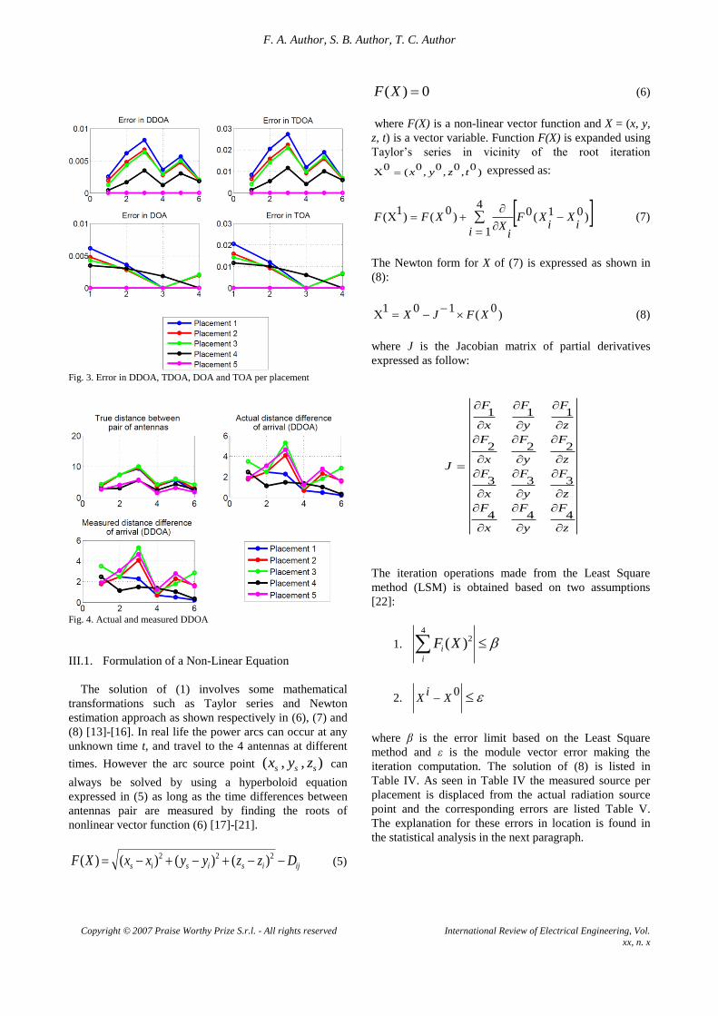
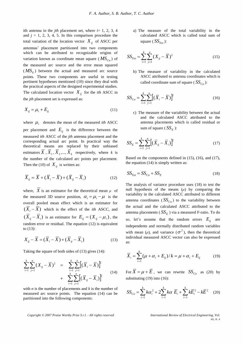
The results shown in Table I are directly obtained from

the distance calculation using the antennas and actual

source 3D Cartesian coordinates. While the values listed

in Table II are calculated using the measured signal data

when the arc source coordinates have been derived from

the solution of (1). The values of the signal distance of

arrival (DOA) listed in Table III and IV are directly

proportional to the values of respectively illustrated in

Tables I and II by a constant c (which is assumed to be

the speed of light) and they are defined as signal time of

arrival (TOA). From the values of Table III the actual

time difference of arrival (TDOA) between the antennas

are calculated and listed in Table XI (see appendix). The

actual distances between pair of antennas are calculated

using their corresponding Cartesian coordinates and the

results are illustrated in Table VII (see appendix). From

Table VII are derived the actual time between antennas

pair as shown in Table XII (see appendix). The measured

signal time difference of arrival obtained from the cross-

correlation function discussed above are presented in

Table X. From these measured TDOA values we

obtained the corresponding measured distance difference

of arrival (DDOA) as shown in Tables IX (see appendix).

Finally the measured distances and times are compared

with actual values and the outcome error results observed

are shown in the appendix in Tables XIII, XIV and XV.

These errors show clearly that the actual and measured

values are quite close as it can be observed in Figures 2

and 3. In order to distinguish the actual time between the

antennas from the TDOA it can be seen that if two

antennas are placed at the same distance from the

radiation source, they will have a TDOA equals to zero.

This means that two antennas placed at the same distance

from the source have no time delay in the traveling wave

they receive from the radiation source.

TABLE I

ACTUAL DISTANCE OF ARRIVAL (DOA) [m]

Placement 1d 2d 3d 4d

1 12.215 10.424 9.748 9.949

2 12.214 10.423 9.748 8.128

3 12.213 8.700 9.748 6.902

4 11.211 8.735 10.09 9.748

5 5.110 6.988 8.193 9.748

TABLE II

MEASURED DISTANCE OF ARRIVAL (DOA) [m]

Placement 1d 2d 3d 4d

1 12.209 10.420 9.748 9.951

2 12.209 10.420 9.748 8.130

3 12.209 8.697 9.748 6.904

4 11.208 8.732 10.089 9.748

5 5.110 6.988 8.193 9.748

TABLE III

ACTUAL TIME OF ARRIVAL TOA [ns]

Placement 1t 2t 3t 4t

1 40.716 34.745 32.495 33.165

2 40.712 34.742 32.495 27.095

3 40.710 29.002 32.495 23.007

4 37.371 29.116 33.637 32.495

5 17.033 23.293 27.309 32.495

TABLE IV

MEASURED TIME OF ARRIVAL TOA [ns]

Placement 1t 2t 3t 4t

1 40.696 34.733 32.495 33.158

2 40.696 34.733 32.495 27.101

3 40.696 28.992 32.495 23.014

4 37.359 29.105 33.631 32.495

5 17.033 23.294 27.309 32.495

One should note that TDOA is different from the actual

time between the antennas as the first term is based on the

concept of signal traveling time while the latter is the

ratio of the actual distance between pair of antennas and

the speed of light.



xx, n. x

Fig. 3. Error in DDOA, TDOA, DOA and TOA per placement

Fig. 4. Actual and measured DDOA

III.1. Formulation of a Non-Linear Equation

The solution of (1) involves some mathematical

transformations such as Taylor series and Newton

estimation approach as shown respectively in (6), (7) and

(8) [13]-[16]. In real life the power arcs can occur at any

unknown time t, and travel to the 4 antennas at different

times. However the arc source point ),,( sss zyx can

always be solved by using a hyperboloid equation

expressed in (5) as long as the time differences between

antennas pair are measured by finding the roots of

nonlinear vector function (6) [17]-[21].

ijisisis DzzyyxxXF 222 )()()()( (5)

0)( XF (6)

where F(X) is a non-linear vector function and X = (x, y,

z, t) is a vector variable. Function F(X) is expanded using

Taylor’s series in vicinity of the root iteration

)0

,0

,0

,0

(0

tzyx expressed as:

)01(04

1

)0

()1

(i

Xi

XF

i iX

XFF

(7)

The Newton form for X of (7) is expressed as shown in

(8):

)0

(101

XFJX

(8)

where J is the Jacobian matrix of partial derivatives

expressed as follow:

z

F

y

F

x

F

z

F

y

F

x

F

z

F

y

F

x

F

z

F

y

F

x

F

J

444

333

222

111

The iteration operations made from the Least Square

method (LSM) is obtained based on two assumptions

[22]:

1. 4

2)(i

i XF

2. 0

Xi

X

where β is the error limit based on the Least Square

method and ε is the module vector error making the

iteration computation. The solution of (8) is listed in

Table IV. As seen in Table IV the measured source per

placement is displaced from the actual radiation source

point and the corresponding errors are listed Table V.

The explanation for these errors in location is found in

the statistical analysis in the next paragraph.



xx, n. x

TABLE IV

ARC SOURCE POSITION Placement Actual source Measured source

x y z x y z

1 0.073 8.89 5.1 0.01025 8.88998 5.09999

2 0.073 8.89 5.1 0.00794 8.88999 5.09999

3 0.073 8.89 5.1 0.00709 8.88999 5.1

4 0.073 8.89 5.1 0.00709 8.88999 5.1

5 0.073 8.89 5.1 0.0177 8.88994 5.09997

TABLE V

ERROR IN ASCC Placement x y z

1 0.06275 0.00098 0.00099

2 0.06506 0.00099 0.00099

3 0.06591 0.00099 0.001

4 0.06591 0.00099 0.001

5 0.05530 0.00094 0.00097

III.2. Statistical Analysis for the Impact of Antenna

Placement

III.2.1. Multiple Linear Regression

The solution of (6) is the arc source 3D Cartesian

coordinates (ASCC). From the Table IV and V it is

observed that the calculated arc source point is slightly

displaced from the actual source. A linear regression in

conjunction with the analysis of variance (ANOVA) is

used to analyze the correlation between the error in the

actual and calculated ASCC and the placement of the

antennas during the experiment. As seen in Table IV the

rows show the different antennas placements and the

columns are the source coordinates. The correlation

between the errors listed in Table V and the antennas

Cartesians coordinates per placement is expressed as:

3322110,, 321XXXY XXX

(9)

where 321 ,, XXXY denotes the response meaning the

errors displayed between the actual and calculated

ASCC. The predictor variables are 1X , 2X and 3X

assuming respectively the values of x-, y- and z-values

of antennas coordinates per placement. The intercept of

the model in (9) is 0 . The coefficients 1 , 2 and 3

are real numbers, the target to be estimated. The variables

presented in (9) are defined as:

5

4

3

2

1

Y

Y

Y

Y

Y

Y ,

3

2

1

0

and

352515

342414

332313

322212

312111

1

1

1

1

1

XXX

XXX

XXX

XXX

XXX

X

with X is a 5x4 matrix, the first member of each row of

this matrix X is 1. The remaining elements of the ith row

for each i consists of the values assumed by the 3

predictor variables that give rise to the response

321 ,, XXXY and i=1, 2, 3, 4 and 5. The linear regression

results are listed in Tables VI. As seen in Table VI for the

linear regression results show R square equals to

0.99988, that is 99.88% of the antennas coordinates are

accounted for by the variation observed in the arc source

as illustrated in Table IV.

TABLE VI

LINEAR REGRESSION Regression Statistics

Multiple R 0.99988

R Square 0.99975

Adjusted R Square 0.49950

Standard Error 0.00625

Observations 5

Coefficients Standard

Error

t Stat

Intercept 0

1X 0.00053 0.00058 0.90946

2X -0.00049 0.00026 -1.89481

3X 0.20980 0.00434 48.3840

III.2.2. Analysis of variance (ANOVA)

The analysis of variance (ANOVA) in conjunction to

the linear regression model is done to analyze the

solution of (6) by comparing the measured arc source

point with the actual source in terms of their Cartesian

coordinates. To do so we need to compare both arc

sources ASCC population means (μ) according to

differently placed antenna sets by testing:

jiH

H

:

:

1

543210 (10)

For some i (which indicates the ith antenna) and j (the jth

antenna placement set) based on independent ASCC

drawn from the antennas’ placements. Let

),,( ijijijij zyxX denotes the calculated ASCC for the



xx, n. x

ith antenna in the jth placement set, where i= 1, 2, 3, 4

and j = 1, 2, 3, 4, 5. In this comparison procedure the

total variation of the location vector ijX of ASCC per

antennas’ placement partitioned into two components

which can be attributed to recognizable origins of

variation known as coordinate mean square ( CoMS ) of

the measured arc source and the error mean squared

( EMS ) between the actual and measured arc source

points. These two components are useful in testing

pertinent hypotheses mentioned (10) since they deal with

the practical aspects of the designed experimental studies.

The calculated location vector ijX for the ith ASCC in

the jth placement set is expressed as:

ijiij EX (11)

where i denotes the mean of the measured ith ASCC

per placement and ijE is the difference between the

measured ith ASCC of the jth antenna placement and the

corresponding actual arc point. In practical way the

theoretical means are replaced by their unbiased

estimators X , 1X , 2X ,..., kX respectively, where k is

the number of the calculated arc points per placement.

Then the (10) of ijX is written as:

)()( iijiij XXXXXX (12)

where, X is an estimator for the theoretical mean μ of

the measured 3D source position, ii is the

overall pooled mean effect which is an estimator for

)( XX i which is the effect of the ith ASCC, and

)( iij XX is an estimator for )( iijij XE , the

random error or residual. The equation (12) is equivalent

to (13):

)()( iijiij XXXXXX

(13)

Taking the square of both sides of (13) gives (14):

k

i

n

j

iij

k

i

n

j

i

k

i

n

j

ij

XX

XXXX

1 1

2

1 1

2

1 1

2

)(

)()(

(14)

with n is the number of placements and k is the number of

measured arc source points. The equation (14) can be

partitioned into the following components:

a) The measure of the total variability in the

calculated ASCC which is called total sum of

square ( TotSS ):

k

i

n

j

ijTot XXSS1 1

2)( (15)

b) The measure of variability in the calculated

ASCC attributed to antenna coordinates which is

called coordinate sum of square ( CoSS ):

k

i

n

j

iCo XXSS1 1

2)( (16)

c) The measure of the variability between the actual

and the calculated ASCC attributed to the

antenna placements which is called residual or

sum of square ( ESS ):

k

i

n

j

iijE XXSS1 1

2)( (17)

Based on the components defined in (15), (16), and (17),

the equation (14) is simply written as:

ECoTot SSSSSS (18)

The analysis of variance procedure uses (18) to test the

null hypothesis of the means (μ) by comparing the

variability in the calculated ASCC attributed to different

antenna coordinates ( CoSS ) to the variability between

the actual and the calculated ASCC attributed to the

antenna placements ( ESS ) via a measured F-ratio. To do

so, let’s assume that the random errors ijE are

independents and normally distributed random variables

with mean (μ), and variance (2 ), then the theoretical

individual measured ASCC vector can also be expressed

as:

ijiiji

k

i

i EkEX

/)(1

(19)

For EX , we can rewrite CoSS

as (20) by

substituting (19) into (16):

2

1

2

11

2 2 EkEkEkkSSk

i

i

k

i

i

k

i

iCo

(20)



xx, n. x

The expectation of CoSS is given as:

k

i

iCo kkSSE1

22)1(

(21)

by dividing (16) by (k – 1) the coordinates mean square

CoMS is obtained as:

)1/( kSSMS CoCo (22)

Similarly to obtain the unbiased estimator for the

variance 2 of the calculated ASCC, ESS is divided by

(N – k) where N is the total number of observations per

placements, resulting in so called error mean squared

EMS as:

)/( kNSSMS EE (23)

And finally the values of CoMS and EMS are used to

make a 0H

0H is true when F-ratio 1/ ECo MSMS

0H is not true when F-ratio 1/ ECo MSMS

The entire results of ANOVA analysis is presented in

Table XVI (see appendix).

An experimental set-up for the arc source location and

the interpretations of the results of the calculated ASCC

statistics analysis are the main subject of the next section.

IV. Arc Location Experiment

In order to evaluate the performance of the proposed

algorithm, we performed a set of arc location experiments

as shown in Figures 5 and 7. As seen in Figure 7 we

present 2 types of topologies in term of antennas

placements such as horizontally and vertically placed

antennas. These two types of placements will help to

choose the suitable antennas arrangement that could be

adopted for power arc fault detection in power

distribution network.

IV.1. Experiment set-up

The experiment set-up consisted of four antennas

placed at known distances from the arc source. The

antennas were connected through coaxial cable of 3 m to

a multichannel LeCroy digitizer of 2 GHz sampling rate.

As for arc staging, a pine tree of total height 9 m was lent

on a metallic rod (as a conductor) to make an arcing

contact at about 5.1 m above the floor as shown in Figure

5 in which the antennas are labeled as 1ant , 2ant , 3ant

and 4ant .

Fig. 5. The antennae used are Yagi – Uda (Yagi) antennae which cover

a frequency range of 47 - 862 GHz.

The antennas used are Yagi – Uda (Yagi) antennas

which cover a frequency range of 47 - 862 GHz. As seen

in Figure 7 the placements 1 to 4 show that the antennas

are horizontally configured, when in placement 5 they are

vertically placed. The arc current passing through the rod

was also recorded. It was determined that the tree had a

resistance of 316 k. The signals were captured at the

sample rate of 20000 samples per microsecond. A total of

100 measurements were made with N = 20 observations

per antenna placement. A high voltage AC source of 20

kV was used to generate the power arcs and the supplied

voltage levels used for placement 1, 2, 3, 4 and 5 are

respectively 3.925, 3.46, 3.415, 2.84 and 2.705 kV.

Figure 6 shows the signals captured by the 4 antennas

connected to the digitizer during the experiment. The

current signal passing through the tree is shown above in

Figure 6 and below it are the arc radiation signals

captured by the antennas named iant (with i = 1, 2, 3,

4). In Figure 7, the antennas the antennas close to the arc

source point are considered as reference points such as

antennas 3 and 4 respectively for the placement 1 and 2.

Placement 3 and 4 present slightly similar configuration

but the reference antenna is placed in different location,

where the antenna 4 is used as reference point in

placement 3 and the antenna 2 is the reference point of

placement 4. Finally the antennas configuration is

changed to a vertical position in placement 5 with

antenna 1 used as reference point. From these 5 different



xx, n. x

placements, the signal time and distance difference of

arrival are calculated as discussed above. The algorithm

Fig. 6. The captured arc RF signal and the arc current

Fig. 7. Antennas placements

of the arc source point location derived from the captured

signal data is explained in the next paragraph.

IV.2. Arc Source Location Results

The solution of (6) was formed by an application of the

Newton–Raphson technique procedure using Matlab

toolbox. The derivation of the proposed algorithm is

described as follows: A reference point in each of the 5

antenna placements is selected as the location of the

antenna that is closest to the arc source. The reference

antenna indexed as 0 and the other antennas as i = 1, 2,

and 3. The distance between an antenna i to the reference

antenna is then expressed as 00 ddd ii . Let now

iX be the four antennas vector position and compute

2

0

2ddi as:

2

0

22

0

2

ssii XXXXdd (24)

The right side of (24) can be expressed as

2

0

2

0

2

0

222

2

0

2

)()()(

)()()(

sss

sisisi

ssi

zzyyxx

zzyyxx

XXXX

(25)

The left side of (24) is expressed as

ii

ii

ddd

ddddd

00

2

0

2

0

2

00

2

0

2

2

)(

(26)

Substituting (25) and (26) into (24) yields to (27)

)(2

)(2

)(22

0

2

0

2

0

2

0

2

0

2

0

2

00

2

0

zzzzz

yyyyy

xxxxxddd

isi

isi

isiii

(27)

Grouping the known terms in (27) together yields to (29),

then F(X) mentioned before in (6) is expressed as:

)(2

)(2

)(2

)2()(

0

2

0

2

0

2

0

2

0

2

0

2

00

2

0

zzzzz

yyyyy

xxxxx

dddXF

isi

isi

isi

ii

(29)

The solution of (29) is solved as:

UAX s (30)

where



xx, n. x

0

20

10

000

202020

101010

iiii d

d

d

zzyyxx

zzyyxx

zzyyxx

A

Tsss

T

s dzzyyxxX 0000

Ti

T uuuU 00201

Note that 2

0

22

002

1iii dddu

and the calculated

arc source Cartesian coordinates vector sX is calculated

as:

UAXUAX ss

1 (31)

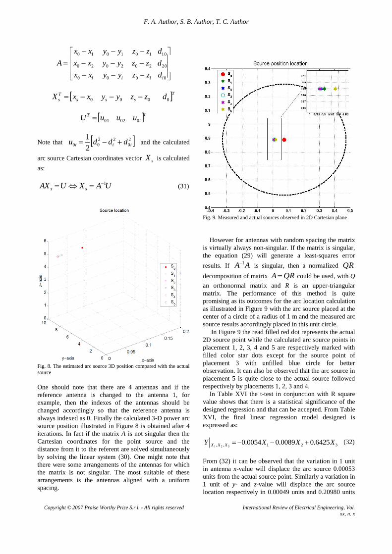
Fig. 8. The estimated arc source 3D position compared with the actual

source

One should note that there are 4 antennas and if the

reference antenna is changed to the antenna 1, for

example, then the indexes of the antennas should be

changed accordingly so that the reference antenna is

always indexed as 0. Finally the calculated 3-D power arc

source position illustrated in Figure 8 is obtained after 4

iterations. In fact if the matrix A is not singular then the

Cartesian coordinates for the point source and the

distance from it to the referent are solved simultaneously

by solving the linear system (30). One might note that

there were some arrangements of the antennas for which

the matrix is not singular. The most suitable of these

arrangements is the antennas aligned with a uniform

spacing.

Fig. 9. Measured and actual sources observed in 2D Cartesian plane

However for antennas with random spacing the matrix

is virtually always non-singular. If the matrix is singular,

the equation (29) will generate a least-squares error

results. If AA 1 is singular, then a normalized QR

decomposition of matrix QRA could be used, with Q

an orthonormal matrix and R is an upper-triangular

matrix. The performance of this method is quite

promising as its outcomes for the arc location calculation

as illustrated in Figure 9 with the arc source placed at the

center of a circle of a radius of 1 m and the measured arc

source results accordingly placed in this unit circle.

In Figure 9 the read filled red dot represents the actual

2D source point while the calculated arc source points in

placement 1, 2, 3, 4 and 5 are respectively marked with

filled color star dots except for the source point of

placement 3 with unfilled blue circle for better

observation. It can also be observed that the arc source in

placement 5 is quite close to the actual source followed

respectively by placements 1, 2, 3 and 4.

In Table XVI the t-test in conjunction with R square

value shows that there is a statistical significance of the

designed regression and that can be accepted. From Table

XVI, the final linear regression model designed is

expressed as:

321,, 6425.00089.00054.0321

XXXY XXX

(32)

From (32) it can be observed that the variation in 1 unit

in antenna x-value will displace the arc source 0.00053

units from the actual source point. Similarly a variation in

1 unit of y- and z-value will displace the arc source

location respectively in 0.00049 units and 0.20980 units



xx, n. x

from the actual source point. The coefficient 0.20980 of

the explanatory variable 3X (the antennas z-coordinate)

is quite too large compared to the coefficients of x and y.

This large coefficient observed in z- value is due to the

fact that the antennas height of 1.1 m is too close to the

floor level causing the signal to be reflected by the floor.

The answer is found in the ANOVA statistics results as

discussed below.

It can be said from Table XVI that the null hypothesis

for the 5 antennas’ placements cannot be rejected since

their corresponding F-ratio are close to 1. This means

that there is strong evidence that the antennas placement

is significant in calculation errors in arc source location.

But the F-ratios of the antennas Cartesian coordinates per

placement is larger than 1. Therefore F-ratio indicates

that there is no statistical evidence of the differences

observed in the antennas different location. Then the

comparison of their corresponding variance (2 )

required in order to test the 1H hypothesis. That will tell

the exact percentage errors attributed to the antennas

coordinates. From the ANOVA results listed in Table

XVI, the unbiased estimates for the variance of the

antennas coordinates attributed to the antennas coordinate

in placement 1 is as follows:

265.4ˆ 2 EMS

1875.0

20/)265.40144.8(

/)(ˆ0

2

nMSMS ECoCo

The estimated total error due to the antennas’ coordinates

is:

4524.4)ˆˆ(ˆ 222 CoTot

The proportion of total error in antennas' coordinates due

to the placements is:

441.0ˆ/ˆ 22 TotCo

That is 4.21 % of total error observed in antennas’

coordinates attributed to the antennas location. Similarly

the estimated total errors observed in placement 1 are 0

%. Based on these statistical evidences we conclude that

the method of cross-correlation approach for arc source

location depends on the antennas’ placements. From the

linear regression model and the ANOVA analysis, it is

observed that the antennas heights are too low and their

proximity from the floor level causes the signal reflection

from the floor is affecting the location accuracy with an

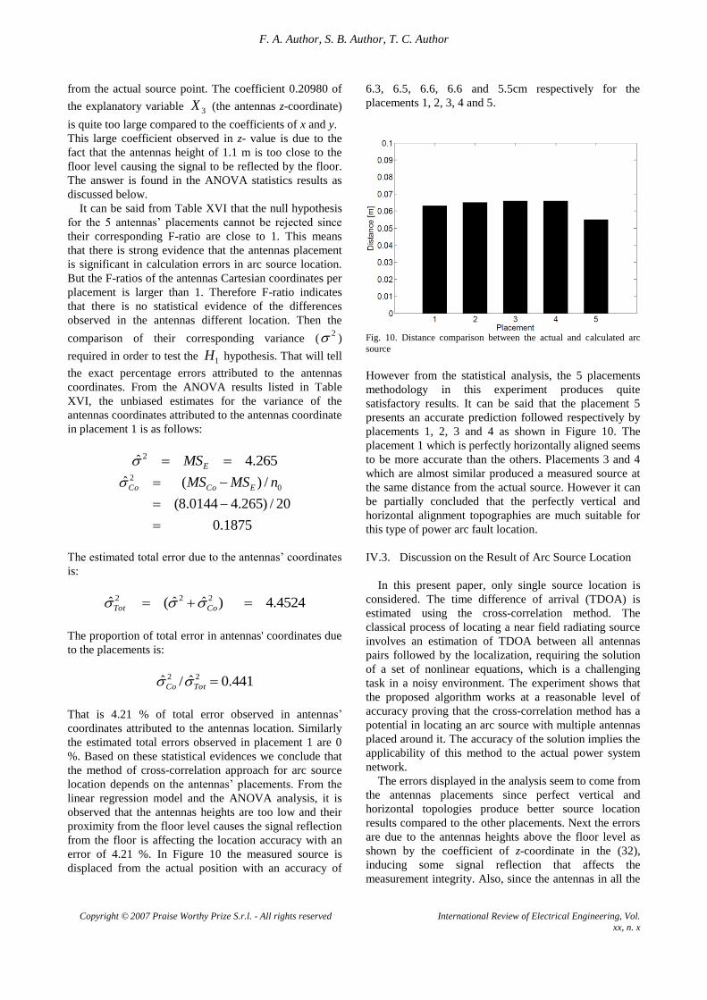
error of 4.21 %. In Figure 10 the measured source is

displaced from the actual position with an accuracy of

6.3, 6.5, 6.6, 6.6 and 5.5cm respectively for the

placements 1, 2, 3, 4 and 5.

Fig. 10. Distance comparison between the actual and calculated arc

source

However from the statistical analysis, the 5 placements

methodology in this experiment produces quite

satisfactory results. It can be said that the placement 5

presents an accurate prediction followed respectively by

placements 1, 2, 3 and 4 as shown in Figure 10. The

placement 1 which is perfectly horizontally aligned seems

to be more accurate than the others. Placements 3 and 4

which are almost similar produced a measured source at

the same distance from the actual source. However it can

be partially concluded that the perfectly vertical and

horizontal alignment topographies are much suitable for

this type of power arc fault location.

IV.3. Discussion on the Result of Arc Source Location

In this present paper, only single source location is

considered. The time difference of arrival (TDOA) is

estimated using the cross-correlation method. The

classical process of locating a near field radiating source

involves an estimation of TDOA between all antennas

pairs followed by the localization, requiring the solution

of a set of nonlinear equations, which is a challenging

task in a noisy environment. The experiment shows that

the proposed algorithm works at a reasonable level of

accuracy proving that the cross-correlation method has a

potential in locating an arc source with multiple antennas

placed around it. The accuracy of the solution implies the

applicability of this method to the actual power system

network.

The errors displayed in the analysis seem to come from

the antennas placements since perfect vertical and

horizontal topologies produce better source location

results compared to the other placements. Next the errors

are due to the antennas heights above the floor level as

shown by the coefficient of z-coordinate in the (32),

inducing some signal reflection that affects the

measurement integrity. Also, since the antennas in all the



xx, n. x

placement sets, are quite close to each other, it seems to

influence the signal integrity and add an additional source

of error.

V. CONCLUSION

This paper reported an experimental investigation of

power arc source location using radio frequency

measurements. A digitizer equipped with the antennas

and connected to a PC proved to be a useful device in

power arcing fault detection and location. According to

the measurements it seems that electromagnetic radiation

from an arc source point can be evaluated by measuring

the signals in time domain. The difference between signal

wave times of arrival can help with power arc source

location. This proposed method could become a useful

technology of the power arc location as well as distance

estimation from the point of view of the cost and

accuracy.

The proposed source localization realized based on

time delay of arrival (TDOA) estimation using antenna

array, proved accurate and efficient. Of course,

measurements of power arcs on-site will be disturbed by

different noises. Therefore, it might be useful to create a

database of different signals, which could serve for

pattern recognition purpose, and that will be the main

topic of our future research paper. This paper has

introduced an improved power arc location determination

system where the time difference of arriving signals can

be determined using cross-correlation method. When

used in conjunction with a suitable location algorithm,

the errors associated with the location of an arcing fault

source need to be further reduced; therefore our future

works will investigate the arc fault location using other

types of fault detection algorithms.

Appendix

TABLE VII

ACTUAL DISTANCE BETWEEN THE ANTENNAS [m] Placement

12d 13d 14d 23d 24d 34d

1 3.670 7.350 9.350 3.680 5.680 2.000

2 3.670 7.350 9.583 3.680 6.056 2.900

3 4.228 7.350 10.03 4.237 5.883 4.145

4 2.746 2.930 5.530 2.399 4.307 2.600

5 2.550 3.970 5.710 1.420 3.160 1.740

TABLE VIII

ACTUAL DDOA BETWEEN THE ANTENNAS [m] Placement

12d 13d 14d 23d 24d 34d

1 1.791 2.467 2.266 0.675 0.474 0.201

2 1.791 2.465 4.085 0.674 2.294 1.620

3 3.513 2.465 5.311 1.048 1.798 2.846

4 2.477 1.120 1.463 1.356 1.014 0.343

5 1.878 3.083 4.638 1.205 2.760 1.556

TABLE IX

MEASURED DDOA BETWEEN THE ANTENNAS [m] Placement

12d 13d 14d 23d 24d 34d

1 1.789 2.460 2.257 0.671 0.468 0.203

2 1.789 2.460 4.078 0.671 2.289 1.618

3 3.511 2.460 5.305 1.051 1.793 2.844

4 2.476 1.119 1.459 1.358 1.017 0.341

5 1.878 3.083 4.638 1.205 2.760 1.556

TABLE X

MEASURED TIME DIFFERENCE OF ARRIVAL BETWEEN THE

ANTENNAS (TDOA) [ns] Placement

12t 13t 14t 23t 24t 34t

1 5.963 8.201 7.524 2.238 1.561 0.677

2 5.963 8.201 13.594 2.238 7.632 5.393

3 11.704 8.201 17.682 3.503 5.978 9.481

4 8.254 3.728 4.864 4.525 3.389 1.136

5 6.260 10.276 15.461 4.016 9.201 5.185

TABLE XI

ACTUAL TIME DIFFERENCE OF ARRIVAL BETWEEN THE

ANTENNAS (TDOA) [ns] Placement

12t 13t 14t 23t 24t 34t

1 5.971 8.222 7.552 2.250 1.580 0.670

2 5.970 8.217 13.617 2.248 7.647 5.400

3 11.709 8.215 17.703 3.493 5.995 9.488

4 8.255 3.734 4.876 4.521 3.379 1.142

5 6.260 10.276 15.461 4.016 9.201 5.185

TABLE XII

ACTUAL TIME BETWEEN THE ANTENNAS [ns] Placement

12t 13t 14t 23t 24t 34t

1 12.23 24.5 31.167 12.267 18.933 6.667

2 12.23 24.5 31.943 12.267 20.186 9.667

3 14.09 24.5 33.433 14.123 19.608 13.82

4 9.155 9.767 18.433 7.997 14.356 8.667

5 8.5 13.233 19.033 4.733 10.533 5.8

TABLE XIII

ERROR IN TDOA [ns] Placement

12e 13e 14e

1 0.00850 0.02057 0.02743

2 0.00659 0.01595 0.02246

3 0.00423 0.01424 0.02108

4 0.00148 0.00557 0.01167

5 0.00005 0.00006 0.00007

Placement 23e 24e 34e

1 0.01206 0.01893 0.00686

2 0.00935 0.01587 0.00651

3 0.01001 0.01685 0.00684

4 0.00409 0.01018 0.00609

5 0.00001 0.00002 0.00001



xx, n. x

TABLE XIV

ERROR IN DOA [m] Placement

1e 2e 3e 4e

1 0.00615 0.00360 0.00002 0.00208

2 0.00477 0.00280 0.00001 0.00196

3 0.00426 0.00299 0.00001 0.00206

4 0.00349 0.00305 0.00182 0.00001

5 0.00003 0.00004 0.00004 0.00005

TABLE XV

ERROR IN TOA [ns] Placement

1e 2e 3e 4e

1 0.02051 0.01201 0.00005 0.00692

2 0.01591 0.00932 0.00003 0.00654

3 0.01421 0.00998 0.00003 0.00687

4 0.01164 0.01016 0.00607 0.00003

5 0.00009 0.00014 0.00015 0.00016

TABLE XVI

ANOVA RESULTS Source of

Variation

SS df MS F

Placement 1 12,79492 3 4,264973 1

Coordinates 24,04317 3 8,01439 1,879119

Error 38,38476 9 4,264973

Total 75,22285 15

Placement 2 18,09217 3 6,030723 1,491317

Coordinates 26,02257 3 8,67419 2,145011

Error 36,39501 9 4,04389

Total 80,50974 15

Placement 3 21,37333 3 7,124442 1,636339

Coordinates 33,33459 3 11,11153 2,552092

Error 39,18503 9 4,353892

Total 93,89294 15

Placement 4 4,033869 3 1,344623 0,785354

Coordinates 39,66071 3 13,22024 7,721546

Error 15,40911 9 1,712123

Total 59,10368 15

Placement 5 4,368569 3 1,45619 1

Coordinates 18,49807 3 6,166023 4,234355

Error 13,10571 9 1,45619

Total 35,97234 15

Acknowledgements

The authors gratefully acknowledge the contributions

of Tatu Nieminen and Joni Klüss, for their work on

building the laboratory experiment.

References

[1] Bartlett, E.J.; Moore, P.J.; “Remote sensing of power system

arcing faults”, Advances in Power System Control, Operation

and Management, 2000. APSCOM-00. 2000 International

Conference on Vol. 1 , 2000, pp. 49–53.

[2] Moore, P.J.; Portugues, I.E.; Glover, I.A.; “Radiometric location

of partial discharge sources on energized high-Voltage plant”,

Power Delivery, IEEE Transactions on Vol. 20, 2005, pp. 2264-

2272.

[3] Shihab, S.; Wong, K.L.; “Detection of faulty components on

power lines using radio frequency signatures and signal

processing techniques”, Power Engineering Society Winter

Meeting, 2000. IEEE Vol. 4, 2000, pp. 2449–2452.

[4] Young, D.P.; Keller, C.M.; Bliss, D.W.; Forsythe, K.W.; “Ultra-

wideband (UWB) transmitter location using time difference of

arrival (TDOA) techniques”, Signals, Systems and Computers,

2003. Conference Record of the Thirty-Seventh Asilomar

Conference on Vol. 2 , 2003, pp. 1225–1229.

[5] Sun, Y.; Stewart, B.G.; Kemp, I.J.; “Alternative cross-

correlation techniques for location estimation of PD from RF

signal”, Universities Power Engineering Conference, 2004.

UPEC 2004. 39th International Vol. 1, 2004, pp. 143–148.

[6] Chye Huat Peck; Moore, P.J.; “A direction-finding technique for

wide-band impulsive noise source”, Electromagnetic

Compatibility, IEEE Transactions on Vol. 43, 2001, pp. 149–

1544.

[7] Yang, L.; Judd, M.D.; Bennoch, C.J.; “Time delay estimation for

UHF signals in PD location of transformers [power

transformers]”, Electrical Insulation and Dielectric Phenomena,

2004. CEIDP '04. 2004 Annual Report Conference, 2004, pp.

414-417.

[8] Azaria, M.; Hertz, D.; “IEEE Transactions on Acoustics, Speech,

and Signal Processing”, Vol. 32, 1984, pp. 280-285.

[9] Soeta, Y.; Uetani, S.; Ando, Y.; “Autocorrelation and cross-

correlation analyses of alpha waves in relation to subjective

preference of a flickering light”, Engineering in Medicine and

Biology Society, 2001. Proceedings of the 23rd Annual

International Conference of the IEEE Vol. 1, 2001, pp. 635– 638.

[10] Alavi, B.; Pahlavan, K.; “Modeling of the TOA-based distance

measurement error using UWB indoor radio measurements”,

Communications Letters, IEEE Vol. 10, 2006, pp. 275–277.

[11] Mallat, Achraf; Louveaux, J.; Vandendorpe, L.; “UWB based

positioning: Cramer Rao bound for Angle of Arrival and

comparison with Time of Arrival”, 2006 Symposium on

Communications and Vehicular Technology, pp. 65–68.

[12] Alsindi, N.; Xinrong Li; Pahlavan, K.; “Analysis of Time of

Arrival Estimation Using Wideband Measurements of Indoor

Radio Propagations”, Instrumentation and Measurement, IEEE

Transactions on Vol. 56, 2007, pp. 1537-1545.

[13] Rohrig, C., Kunemund, F., “Mobile Robot Localization using

WLAN Signal Strengths”. Intelligent Data Acquisition and

Advanced Computing Systems: Technology and Applications,

2007. IDAACS 2007. 4th IEEE Workshop, pp. 704 - 709

[14] Bo-Chieh Liu, Ken-Huang Lin “Accuracy Improvement of SSSD

Circular Positioning in Cellular Networks”. Vehicular

Technology, IEEE Transaction, pp. 1766 - 1774

[15] Motter, P. , Allgayer, R.S. ; Muller, I. ; Pereira, C.E. ; Pignaton

de Freitas, E. “Practical issues in Wireless Sensor Network

localization systems using received signal strength indication”.

Sensors Applications Symposium (SAS), 2011 IEEE, pp. 227 -

232

[16] Chih-Chun Lin, She-Shang Xue; Yao, L. “Position Calculating

and Path Tracking of Three Dimensional Location System Based

on Different Wave Velocities”. Dependable, Autonomic and

Secure Computing, 2009. DASC '09. Eighth IEEE International

Conference, pp. 436 - 441

[17] El Arja, H., Huyart, B.; Begaud, X. “Joint TOA/DOA

measurements for UWB indoor propagation channel using

MUSIC algorithm”. Wireless Technology Conference, 2009, pp.

124 - 127

[18] Born, A.,Schwiede, M. ; Bill, R. “On distance estimation based

on radio propagation models and outlier detection for indoor

localization in Wireless Geosensor Networks”, Indoor

Positioning and Indoor Navigation (IPIN), International

Conference 2010, pp. 1 - 6

[19] Fugen Su, Weizheng Ren; Hongli Jin, “Localization Algorithm

Based on Difference Estimation for Wireless Sensor Networks”.

Communication Software and Networks. ICCSN '09.

International Conference, 2009, pp. 499 - 503



xx, n. x

[20] Bing-Fei Wu , Cheng-Lung Jen ; Kuei-Chung Chang, “Neural

fuzzy based indoor localization by Kalman filtering with

propagation channel modeling”. Systems, Man and Cybernetics.

ISIC. IEEE International Conference, 2007, pp. 812 - 817

[21] Benkic, K., Malajner, M.; Planinsic, P.; Cucej, Z. “Using RSSI

value for distance estimation in wireless sensor networks based

on ZigBee”. Systems, Signals and Image Processing, 2008. 15th

International Conference, 2008, pp. 303 - 306

[22] Suk-Un Yoon, Liang Cheng; Ghazanfari, E.; Pamukcu, S.;

Suleiman, M.T. “A Radio Propagation Model for Wireless

Underground Sensor Networks”. Global Telecommunications

Conference (GLOBECOM 2011), 2011, pp. 1 – 5

Authors’ information

Frank Zoko Ble obtained a B.Sc. in

Physics in Ivory coast National University,

Abidjan in 1997. He received M.Sc. in

Electrical Engineering in Helsinki University of

Technology (TKK), Espoo, Finland in 2010.

Currently he is working toward his PhD degree

in Aalto University, School of Electrical

Engineering. His research interests are in

electric power arcs detection using radio frequency measurements.

He is a researcher in the Department of Electrical of Aalto

University, School of Electrical Engineering, Finland.

Matti Lehtonen (1959) was with VTT

Energy, Espoo, Finland from 19987 to 2003,

and since 1999 has been a professor at the

Helsinki University of Technology (TKK),

where he is now head of Electrical

Engineering department. Matti Lehtonen

received both his Master’s and Licentiate

degrees in Electrical Engineering from

Helsinki University of Technology , in 1984 and 1989 respectively,

and the Doctor of Technology degree from Tampere University of

technology in 1992. The main activities of Professor Lehtonen include

power system planning and asset management, power system

protection including earth fault problems, harmonic related issues and

applications of information technology in distribution systems. He is a

Professor in Aalto University, School of Electrical Engineering,

Finland.

Charles Kim received a PhD degree in

electrical engineering from Texas A&M

University (College Station, TX) in 1989.

Since 1999, he has been with the Department

of Electrical and Computer Engineering at

Howard University. Previously, Dr. Kim held

teaching and research positions at Texas

A&M University and the University of

Suwon. Dr. Kim’s research includes failure detection, anticipation, and

system safety analysis in safety critical systems in energy, aerospace,

and nuclear industries. Several inventions of his in the research area

have been patent field through the university’s intellectual property

office. Dr. Kim is a senior member of IEEE and the chair of an IEEE

chapter in Washington Baltimore section.

Ari Sihvola was born on October 6th,

1957, in Valkeala, Finland. He received the

degrees of Diploma Engineer in 1981,

Licentiate of Technology in 1984, and Doctor

of Technology in 1987, all in Electrical

Engineering, from the Helsinki University of

Technology (TKK), Finland. Besides working

for TKK and the Academy of Finland, he was

visiting engineer in the Research Laboratory of Electronics of the

Massachusetts Institute of Technology, Cambridge, in 1985–1986,

and in 1990–1991, he worked as a visiting scientist at the

Pennsylvania State University, State College. In 1996, he was visiting

scientist at the Lund University, Sweden, and for the academic year

2000–01 he was visiting professor at the Electromagnetic and

Acoustics Laboratory of the Swiss Federal Institute of Technology,

Lausanne. In the summer of 2008, he was visiting professor at the

University of Paris XI, France. Ari Sihvola is professor of

electromagnetic in Aalto University School of Electrical Engineering

(former name before 2010: Helsinki University of Technology) with

interest in electromagnetic theory, complex media, materials modeling,

remote sensing, and radar applications. He is Chairman of the Finnish

National Committee of URSI (International Union of Radio

Science) and Fellow of IEEE. He also served as the Secretary of the

22nd European Microwave Conference, held in August 1992, in Espoo,

Finland. He was awarded the ve-year Finnish Academy Professor

position starting August 2005. He is also director of the Finnish

Graduate School of Electronics, Telecommunications, and Automation

(GETA).

cross correlation method for power arcing source location2)p440-452... · to use a...

Documents