Technical FeaTure

Cross Correlation in Phase noise analysis

Phase noise is a property of an oscillator that can extend in magnitude from the carrier of several volts down to a mere

nano-volt far from the carrier. In many cases the lowest noise OCXOs, SAWs and other spe-cialty oscillators have carrier to noise ratios in excess of -180 dBc/√Hz. The noise level of these oscillators often extends below that of even the mixers and low noise amplifiers at baseband. Cross correlation is a method used in phase noise analysis to extend the range of any single channel measurement by introduc-ing a second channel and utilizing signal pro-cessing to locate the noise that is common to the DUT, yet uncommon to each individual channel. With this method, a typical noise floor improvement of 20 dB is very realistic, allowing for high accuracy measurements of extremely low noise oscillators. This article presents the mathematics with an example of how cross cor-relation can accurately identify signals or noise that is below the level of the measurement in-strument.

Most phase noise measurement systems use what is called carrier cancellation. Phase noise is not measured directly, but down-converted to baseband. In an absolute phase noise mea-surement, where the absolute noise level of an oscillator is being measured, two oscillators are phase locked to one another. Once the two sig-nals are locked with a mixer, the phase noise

of both channels is down-converted directly to baseband without the carrier which is at DC and cancelled.

In a residual or additive phase noise mea-surement, whereby the additive noise of a com-ponent such as an amplifier is to be measured, the oscillator is split into two parts. One path drives the LO port of the mixer while the other path goes through the DUT prior to going into the RF port of the mixer. Within the noise level and isolation of the mixer, the carrier and its noise are canceled, being common between the two paths, while the noise of the DUT is measured directly at an offset and its carrier frequency centered at DC.

In both cases, low noise, low frequency tech-niques are then applied to amplify and sample this signal. However, in both cases, noise levels of system components may limit the measure-ment dynamic range or noise floor. In absolute measurements, the reference oscillator typical-ly is the limitation. In additive measurements, even a very good mixer can often contribute as much noise as a low noise DUT.

Cross correlation has been used by NIST for metrology level phase noise measurements for quite some time (see the references for more information or go to www.nist.gov). Through-

Jason BreitbarthHolzworth Instrumentation, Boulder, CO

78 MICROWAVE JOURNAL FEBRUARY 2011

80 MICROWAVE JOURNAL FEBRUARY 2011

Technical FeaTure

Ducommun RF Product Group is an experienced designer and manufacturer of mmW ampliier. Our facility offers standard and custom products covering the Ka to W-Bands. We feature ampliiers speciically for low noise applications, along with a several interface options including waveguide and coax.

Full Band Ampliiers

Low Noise Ampliiers*Broadband Operation*LNA with high P1 Option*State-of-the-art Low Noise Performance

*MMIC based compact design*Watt level output power at millimeter wave*Custom design

*High gain and band width*Single power supply*Low DC power consumption

*Full waveguide band LNA and PA*Cover Ku & K, Ka, Q, U, V, E, W bands*Selection of various outlines

General Purpose Ampliiers

High Power Ampliier

www.Ducommun.com/ rfproducts233301 Wilmington Ave. Carson, CA 90745-6209

Contact our mmW engineers today to discuss speciic requirements at

310.513.7200 or rfsales@ducommun.com

this leaves a dy-namic range of -170 dBc/Hz (about 10 dB below that of the oscillator). A higher power mixer can increase this dynamic range, but shot noise and other effects can become more dominant (such as the com-

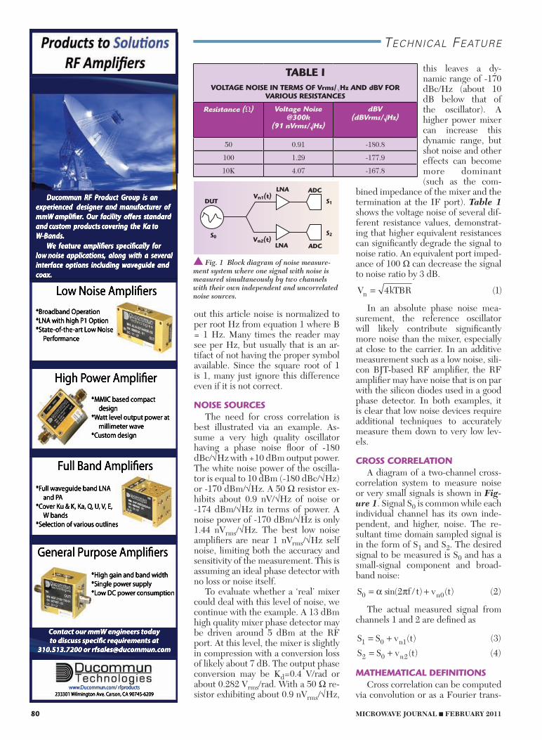
bined impedance of the mixer and the termination at the IF port). Table 1 shows the voltage noise of several dif-ferent resistance values, demonstrat-ing that higher equivalent resistances can significantly degrade the signal to noise ratio. An equivalent port imped-ance of 100 Ω can decrease the signal to noise ratio by 3 dB.

V kTBRn = 4 1( )

In an absolute phase noise mea-surement, the reference oscillator will likely contribute significantly more noise than the mixer, especially at close to the carrier. In an additive measurement such as a low noise, sili-con BJT-based RF amplifier, the RF amplifier may have noise that is on par with the silicon diodes used in a good phase detector. In both examples, it is clear that low noise devices require additional techniques to accurately measure them down to very low lev-els.

CROSS CORRELATIONA diagram of a two-channel cross-

correlation system to measure noise or very small signals is shown in Fig-ure 1. Signal S0 is common while each individual channel has its own inde-pendent, and higher, noise. The re-sultant time domain sampled signal is in the form of S1 and S2. The desired signal to be measured is S0 and has a small-signal component and broad-band noise:

S f t v tn0 02 2= +α πsin( / ) ( ) ( )

The actual measured signal from channels 1 and 2 are defined as

S S v t

S S v tn

n

1 0 1

2 0 2

3

4

= += +

( ) ( )

( ) ( )

MATHEMATICAL DEFINITIONSCross correlation can be computed

via convolution or as a Fourier trans-

out this article noise is normalized to per root Hz from equation 1 where B = 1 Hz. Many times the reader may see per Hz, but usually that is an ar-tifact of not having the proper symbol available. Since the square root of 1 is 1, many just ignore this difference even if it is not correct.

NOISE SOURCESThe need for cross correlation is

best illustrated via an example. As-sume a very high quality oscillator having a phase noise floor of -180 dBc/√Hz with +10 dBm output power. The white noise power of the oscilla-tor is equal to 10 dBm (-180 dBc/√Hz) or -170 dBm/√Hz. A 50 Ω resistor ex-hibits about 0.9 nV/√Hz of noise or -174 dBm/√Hz in terms of power. A noise power of -170 dBm/√Hz is only 1.44 nVrms/√Hz. The best low noise amplifiers are near 1 nVrms/√Hz self noise, limiting both the accuracy and sensitivity of the measurement. This is assuming an ideal phase detector with no loss or noise itself.

To evaluate whether a ‘real’ mixer could deal with this level of noise, we continue with the example. A 13 dBm high quality mixer phase detector may be driven around 5 dBm at the RF port. At this level, the mixer is slightly in compression with a conversion loss of likely about 7 dB. The output phase conversion may be Kd=0.4 V/rad or about 0.282 Vrms/rad. With a 50 Ω re-sistor exhibiting about 0.9 nVrms/√Hz,

s Fig. 1 Block diagram of noise measure-ment system where one signal with noise is measured simultaneously by two channels with their own independent and uncorrelated noise sources.

DUT

ADC

ADCLNA

LNA

S0

Vn1(t)

Vn2(t)

S1

S2

TABLE IVOLTAgE NOISE IN TERMS OF Vrms/Hz AND dBV FOR

VARIOUS RESISTANCES

Resistance () Voltage Noise @300k

(91 nVrms/Hz)

dBV (dBVrms/Hz)

50 0.91 -180.8

100 1.29 -177.9

10K 4.07 -167.8

82 MICROWAVE JOURNAL FEBRUARY 2011

Technical FeaTure

Ducommun RF Product Group is an ex-perienced mmW designer & manufactuer of Mixers, Up & Down Converters, Detec-tors & Multipliers covering Ka- to W-Bands. Ducommun offers a variety of standard or custom designed catalog items that will meet any of your requirements. Our goal is to provide the right solution for your project.

Mixers*Single end balance*Fundamental harmonic*Up to 110Ghz, full WG Band operation

*I/Q Modulation and Demodulation*Low conversion loss & LO power

Detectors*No mechanical timing*Full WG bandwidth*High sensitivity*Compact size*Zero biased

Converter Assemblies*Custom design*Compact and extreme performance*Frequency range up to 110 GHz

Multipliers*Up to W Band*Active and Passive options

*High output power*Up to full WG Band operation*Low harmonic and spurious

www.Ducommun.com/rfproducts233301 Wilmington Ave. Carson, CA 90745-6209

Contact our mmW engineers today to discuss speciic requirements at

310.513.7200 or rfsales@ducommunc.com

achieve averaging. In a cross-correla-tion system, both the magnitude and phase, or real and imaginary parts of the dot product from the cross cor-relation are vector summed. The dot product of the random noise vectors will eventually achieve a vector sum of zero assuming they are truly random and uncorrelated. The dot product of the small common signal will be in phase and real and eventually be the only signal left.

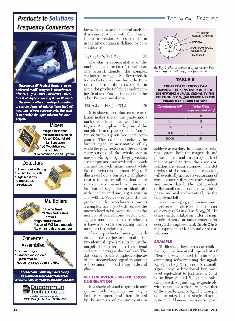
Vector averaging yields a maximum improvement relative to the number of averages (N) in dB as 5log10(N). In other words, it takes an order of mag-nitude increase in measurements for every 5 dB improvement. Table 2 lists the improvement for a number of cor-relations.

EXAMPLETo illustrate how cross correlation

works, a mathematical equivalent of Figure 1 was defined in numerical computing software using the signals S0, S1 and S2. S0 represents a small-signal above a broadband low noise level equivalent to just over a 50 Ω noise floor. S1 and S2 contain noise components vn1 and vn2, respectively, with noise levels that are above that of the small-signal of S0. The example demonstrates that a single channel system could never measure S0, given

form. In the case of spectral analysis, it is easiest to deal with the Fourier transform version. Cross correlation in the time domain is defined by con-volution as

( ) ( ) ( )S S S t S1 2 1 2 5 = − ∗∗

The star is representative of the mathematical function of convolution. The asterisk denotes the complex conjugates of signal S1. Rewritten in terms of a Fourier transform, the Fou-rier transform of the cross correlation is the dot product of the complex con-jugate of one Fourier transform to the other Fourier transform.

F S S F S F S ( )1 2 1 2 6 = ⋅∗

It is shown here that cross corre-lation makes use of the phase infor-mation relative to the two channels. Figure 2 is a phasor diagram of the magnitude and phase of the Fourier transform for a given frequency com-ponent. The red signal vector is the buried signal representative of S0while the gray vectors are the random contributions of the whole system noise levels, S1 or S2. The gray vectors are unique and uncorrelated for each channel for each measurement while the red vector is common. Figure 2 illustrates how a buried signal phasor relates to the overall random noise vectors. Two channels will measure the buried signal vector identically with uncorrelated and larger noise in sum with it. Vector averaging the dot product of the two channels (one as a complex conjugate) will reduce the uncorrelated noise proportional to the number of correlations. Vector aver-aging a number of cross correlations is known as ‘cross correlating’ with a number of correlations.

The dot product of one signal with the complex conjugate of another for two identical signals results in just the magnitude squared of either signal and is real, having a phase of zero. The dot product of the complex conjugate of one uncorrelated signal to another will be random in both magnitude and phase.

VECTOR AVERAgINg THE CROSS CORRELATION

In a single channel magnitude only system, each frequency bin magni-tude is summed and then divided by the number of measurements to

s Fig. 2 Phasor diagram of the vector Fou-rier component of any given frequency.

RMS Vn0

RANDOM NOISEVECTOR(S)

RAM Vn1

‘BURIED’SIGNAL VECTOR

TABLE IICROSS CORRELATIONS CAN

IMPROVE THE SENSITIVITy IN dB OF IDENTIFyINg A SMALL-SIgNAL By THE RELATION 5LOg10(N) wHERE N IS THE

NUMBER OF CORRELATIONS

Correlations (N) Noise Floor Improvement (dB)

1 0

10 5

100 10

1000 15

10000 20

84 MICROWAVE JOURNAL FEBRUARY 2011

Technical FeaTure

> Excellent gain flatness andnoise figure

> Uncompromised input andoutput VSWR

> Very low power consumption> Miniature size and removableconnectors

> Drop-in package for MICintegration

*VSWR 2 : 1 Max for all models* DC +5 V, 60 mA to 150 mA*Noise figure higher @ frequenciesbelow 500 MHz

AMPLIFIERS

SUPER WIDE BAND 0.01 TO 20 GHz

Custom Designs Available

Please call for Detailed Brochures

155 BAYTECH DRIVE, SAN JOSE, CA.95134PH: 408-941-8399 . FAX: 408-941-8388

E-Mail: info@herotek.comWeb Site: www.herotek.comVisa/Master Card Accepted

Other Products: DETECTORS, COMBGENERATORS , LIMITERS, SWITCHES,IMPULSE GENERATORS, INTEGRATED

SUBSYSTEMS

for all applications

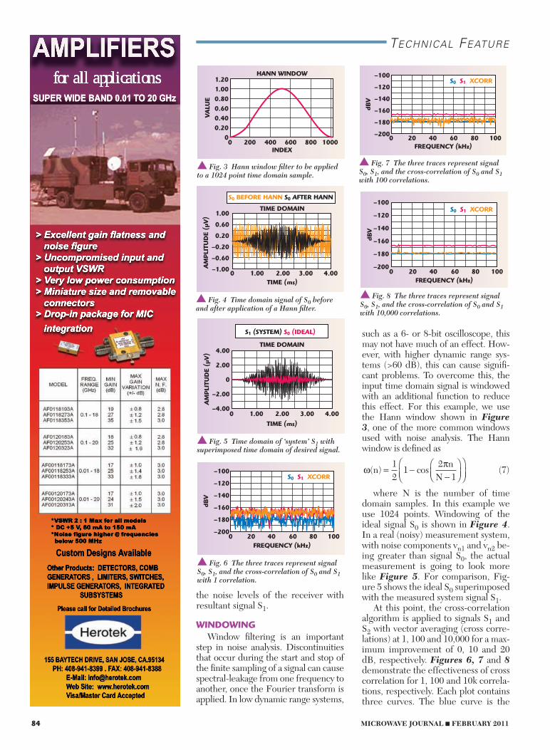
such as a 6- or 8-bit oscilloscope, this may not have much of an effect. How-ever, with higher dynamic range sys-tems (>60 dB), this can cause signifi-cant problems. To overcome this, the input time domain signal is windowed with an additional function to reduce this effect. For this example, we use the Hann window shown in Figure 3, one of the more common windows used with noise analysis. The Hann window is defined as

ω π( ) cos ( )n

nN

= −−

⎛⎝⎜

⎞⎠⎟

⎛⎝⎜

⎞⎠⎟

12

12

17

where N is the number of time domain samples. In this example we use 1024 points. Windowing of the ideal signal S0 is shown in Figure 4. In a real (noisy) measurement system, with noise components vn1 and vn2 be-ing greater than signal S0, the actual measurement is going to look more like Figure 5. For comparison, Fig-ure 5 shows the ideal S0 superimposed with the measured system signal S1.

At this point, the cross-correlation algorithm is applied to signals S1 and S2 with vector averaging (cross corre-lations) at 1, 100 and 10,000 for a max-imum improvement of 0, 10 and 20 dB, respectively. Figures 6, 7 and 8 demonstrate the effectiveness of cross correlation for 1, 100 and 10k correla-tions, respectively. Each plot contains three curves. The blue curve is the

the noise levels of the receiver with resultant signal S1.

wINDOwINgWindow filtering is an important

step in noise analysis. Discontinuities that occur during the start and stop of the finite sampling of a signal can cause spectral-leakage from one frequency to another, once the Fourier transform is applied. In low dynamic range systems,

s Fig. 3 Hann window filter to be applied to a 1024 point time domain sample.

1.201.000.800.600.400.20

010008006004002000

VALU

E

INDEX

HANN WINDOW

s Fig. 4 Time domain signal of S0 before and after application of a Hann filter.

1.00

0.60

0.20

–0.20

–0.60

–1.00AM

PLI

TUD

E (µ

V)

4.003.002.001.000TIME (ms)

TIME DOMAIN

S0 BEFORE HANN S0 AFTER HANN

s Fig. 5 Time domain of ‘system’ S1 with superimposed time domain of desired signal.

AM

PLI

TUD

E (µ

V) 4.00

2.00

0

–2.00

–4.004.003.002.001.000

TIME (ms)

TIME DOMAIN

S1 (SYSTEM) S0 (IDEAL)

s Fig. 6 The three traces represent signal S0, S1, and the cross-correlation of S0 and S1 with 1 correlation.

–100

–120

–140

–160

–180

–200100806040200

dBV

FREQUENCY (kHz)

S0 S1 XCORR

s Fig. 7 The three traces represent signal S0, S1, and the cross-correlation of S0 and S1 with 100 correlations.

–100

–120

–140

–160

–180

–200

dBV

FREQUENCY (kHz)

S0 S1 XCORR

100806040200

s Fig. 8 The three traces represent signal S0, S1, and the cross-correlation of S0 and S1 with 10,000 correlations.

dBV

–100

–120

–140

–160

–180

–200100806040200

FREQUENCY (kHz)

S0 S1 XCORR

Technical FeaTure

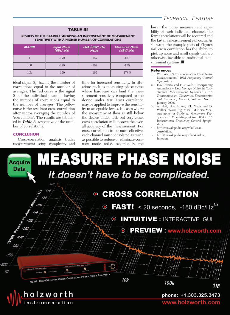
ideal signal S0, having the number of correlations equal to the number of averages. The red curve is the signal S1 of the individual channel, having the number of correlations equal to the number of averages. The yellow curve is the resultant cross correlation after vector averaging the number of ‘correlations’. The results are tabulat-ed in Table 3, respective of the num-ber of correlations.

CONCLUSIONCross-correlation analysis trades

measurement setup complexity and

TABLE IIIRESULTS OF THE EXAMPLE SHOwINg AN IMPROVEMENT OF MEASUREMENT

SENSITIVITy wITH A HIgHER NUMBER OF CORRELATIONS

XCORR Input Noise (dBc/Hz)

LNA (dBV/Hz)Noise

Measured Noise (dBV/Hz)

1 -179 -167 -167

100 -179 -167 -176

10k -179 -167 -178.5

time for increased sensitivity. In situ-ations such as measuring phase noise where hardware can limit the mea-surement sensitivity compared to the device under test, cross correlation may be applied to improve the sensitiv-ity to acceptable levels. In cases where the measurement floor is still below the device under test, but very close, cross correlation will improve the over-all accuracy of the measurement. For cross correlation to be most effective, each channel must be isolated as much as possible to reduce or eliminate com-mon mode noise. Additionally, the

lower the noise measurement capa-bility of each individual channel, the fewer correlations will be required and the faster a measurement can occur. As shown in the example plots of Figures 6-8, cross correlation has the ability to pick up noise and small signals that are otherwise invisible to traditional mea-surement systems.

References1. W.F. Walls, “Cross-correlation Phase Noise

Measurements,” 1992 Frequency Control Symposium.

2. E.N. Ivanov and F.L. Walls, “Interpreting Anomalously Low Voltage Noise in Two-channel Measurement Systems,” IEEE Transactions on Ultrasonics, Ferroelectrics and Frequency Control, Vol. 49, No. 1, January 2002.

3. A. Hati, D.A. Howe, F.L. Walls and D. Walker, “Noise Figure vs. PM Noise Mea-surements: A Study at Microwave Fre-quencies,” Proceedings of the 2003 IEEE International Frequency Control Sympo-sium.

4. http://en.wikipedia.org/wiki/Cross_ correlation.

5. http://en.wikipedia.org/wiki/Window_function.