cross-checking different sources of mobility...

Cross-Checking Different Sources of Mobility InformationMaxime Lenormand1*, Miguel Picornell2, Oliva G. Cantu-Ros2, Antonia Tugores1, Thomas Louail3,4,

Ricardo Herranz2, Marc Barthelemy3,5, Enrique Frıas-Martınez6, Jose J. Ramasco1

1 Instituto de Fısica Interdisciplinar y Sistemas Complejos IFISC (CSIC-UIB), Palma de Mallorca, Spain, 2 Nommon Solutions and Technologies, Madrid, Spain, 3 Institut de

Physique Theorique, CEA-CNRS (URA 2306), Gif-sur-Yvette, France, 4 Geographie-Cites, CNRS-Paris 1-Paris 7 (UMR 8504), Paris, France, 5 Centre d’Analyse et de

Mathematique Sociales, EHESS-CNRS (UMR 8557), Paris, France, 6 Telefonica Research, Madrid, Spain

Abstract

The pervasive use of new mobile devices has allowed a better characterization in space and time of human concentrationsand mobility in general. Besides its theoretical interest, describing mobility is of great importance for a number of practicalapplications ranging from the forecast of disease spreading to the design of new spaces in urban environments. Whileclassical data sources, such as surveys or census, have a limited level of geographical resolution (e.g., districts, municipalities,counties are typically used) or are restricted to generic workdays or weekends, the data coming from mobile devices can beprecisely located both in time and space. Most previous works have used a single data source to study human mobilitypatterns. Here we perform instead a cross-check analysis by comparing results obtained with data collected from threedifferent sources: Twitter, census, and cell phones. The analysis is focused on the urban areas of Barcelona and Madrid, forwhich data of the three types is available. We assess the correlation between the datasets on different aspects: the spatialdistribution of people concentration, the temporal evolution of people density, and the mobility patterns of individuals. Ourresults show that the three data sources are providing comparable information. Even though the representativeness ofTwitter geolocated data is lower than that of mobile phone and census data, the correlations between the populationdensity profiles and mobility patterns detected by the three datasets are close to one in a grid with cells of 262 and 161square kilometers. This level of correlation supports the feasibility of interchanging the three data sources at the spatio-temporal scales considered.

Citation: Lenormand M, Picornell M, Cantu-Ros OG, Tugores A, Louail T, et al. (2014) Cross-Checking Different Sources of Mobility Information. PLoS ONE 9(8):e105184. doi:10.1371/journal.pone.0105184

Editor: Yamir Moreno, University of Zaragoza, Spain

Received April 22, 2014; Accepted July 20, 2014; Published August 18, 2014

Copyright: � 2014 Lenormand et al. This is an open-access article distributed under the terms of the Creative Commons Attribution License, which permitsunrestricted use, distribution, and reproduction in any medium, provided the original author and source are credited.

Data Availability: The authors confirm that, for approved reasons, some access restrictions apply to the data underlying the findings. Twitter data is available todownload using Twitter API (https://dev.twitter.com). The census dataset is public and available on request from the Spanish National Institute for Statistics:(http://www.ine.es). The mobile phone is available on request after negotiation of a non-disclosure agreement with the company. The contact person is EnriqueFrıas-Martınez ([email protected]).

Funding: Partial financial support has been received from the Spanish Ministry of Economy (MINECO) and FEDER (EU) under projects MODASS (FIS2011-24785)and INTENSE@COSYP (FIS2012-30634), and from the EU Commission through projects EUNOIA, LASAGNE and INSIGHT. ML acknowledges funding from theConselleria d’Educacio, Cultura i Universitats of the Government of the Balearic Islands, and JJR from the Ramon y Cajal program of MINECO. The funders had norole in study design, data collection and analysis, decision to publish, or preparation of the manuscript.

Competing Interests: The authors confirm that Jose Javier Ramasco is a PLOS ONE Editorial Board member and this does not alter our adherence to PLOS ONEEditorial policies and criteria. Oliva Garcıa-Cantu, Miguel Picornell, and Ricardo Herranz are employed by Nommon Solutions and Technologies, S.L.. This affiliationdoes not alter the authors’ adherence to all PLOS ONE policies on the sharing of data and materials.

* Email: [email protected]

Introduction

The strong penetration of ICT tools in the society’s daily life is

opening new opportunities for the research in socio-technical

systems [1–3]. Users’ interactions with or through mobile devices

get registered allowing a detailed description of social interactions

and mobility patterns. The sheer size of these datasets opens the

door to a systematic statistical treatment while searching for new

information. Some examples include the analysis of the structure

of (online) social networks [4–13], human cognitive limitations

[14], information diffusion and social contagion [15–19], the role

played by social groups [12,17], language coexistence [20] or even

how political movements raise and develop [21–23].

The analysis of human mobility is another aspect to which the

wealth of new data has notably contributed [24–28]. Statistical

characteristics of mobility patterns have been studied, for instance,

in Refs. [24,25], finding a heavy-tail decay in the distribution of

displacement lengths across users. Most of the trips are short in

everyday mobility, but some are extraordinarily long. Besides, the

travels are not directed symmetrically in space but show a

particular radius of gyration [25]. The duration of stay in each

location also shows a skewed distribution with a few preferred

places clearly ranking on the top of the list, typically corresponding

to home and work [26]. All the insights gained in mobility,

together with realistic data, have been used as proxies for

modeling the way in which viruses spread among people [29] or

among electronic devices [30]. Recently, geolocated data has been

also used to analyze the structure of urban areas [31–38], the

relation between different cities [39] or even between countries

[40].

Most mobility and urban studies have been performed using

data coming essentially from a single data source such as: cell

phone data [5,11,25,26,28,30–38], geolocated tweets [20–22,40],

census-like surveys or commercial information [29]. There is only

a few recent exceptions, for instance, epidemic spreading studies

[41]. When the data has not been generated or gathered ad hoc to

PLOS ONE | www.plosone.org 1 August 2014 | Volume 9 | Issue 8 | e105184

http://creativecommons.org/licenses/by/4.0/

https://dev.twitter.com

http://crossmark.crossref.org/dialog/?doi=10.1371/journal.pone.0105184&domain=pdf

address a specific question, one fair doubt is how much the results

are biased by the data source used. In this work, we compare

spatial and temporal population density distributions and mobility

patterns in the form of Origin-Destination (OD) matrices obtained

from three different data sources for the metropolitan areas of

Barcelona and Madrid. This comparison will allow to discern

whether or not the results are source dependent. In the first part of

the paper the datasets and the methods used to extract the OD

tables are described. In the second part of the paper, we present

the results. First, a comparison of the spatial distribution of users

according to the hour of the day and the day of the week showing

that both Twitter and cell phone data are highly correlated on this

aspect. Then, we compare the temporal distribution of users by

identifying where people are located according to the hour of the

day, we show that the temporal distribution patterns obtained with

the Twitter and the cell phone datasets are very similar. Finally,

we compare the mobility networks (OD matrices) obtained from

cell phone data, Twitter and census. We show that it is possible to

extract similar patterns from all datasets, keeping always in mind

the different resolution limits that each information source may

inherently have.

Materials and Methods

This work is focused on two cities: the metropolitan areas of

Barcelona [42] and Madrid [43] both in Spain and for which data

from the three considered sources is available. The metropolitan

area of Barcelona contains a population of 3,218,071 (2009) within

an area of 636 km2. The population of the metropolitan area of

Madrid is larger, with 5,512,495 inhabitants (2009) within an area

of 1,935 km2 [44]. In order to compare activity and intra mobility

in each city, the metropolitan areas are divided into a regular grid

of square cells of lateral size l (Figure 1b). Two different sizes of

grid cells (l = 1 km and l = 2 km) are considered in order to

evaluate the robustness of the results. Since mobility habits and

population concentration may change along the week, we have

divided the data into four groups: one, from Monday to Thursday

representing a normal working day and three more for Friday,

Saturday and Sunday.

The concentration of phone or Twitter users is quantified by

defining two three dimensional matrices T = (Tg,w,h) and

P = (Pg,w,h), accounting, respectively, for the number of Twitter

users and the number of mobile phone users in the grid cell g at

the hour of the day h and for the group of days w. The index for

cells g runs in the range [1, n]. In the following, details for the

three datasets are more thoroughly described.

1.1 Mobile phone dataThe cell phone data that we are analyzing come from

anonymized users’ call records collected during 55 days (noted

as D hereafter) between September and November 2009. The call

records are registered by communication towers (Base Transceiver

Station or BTS), identified each by its location coordinates. The

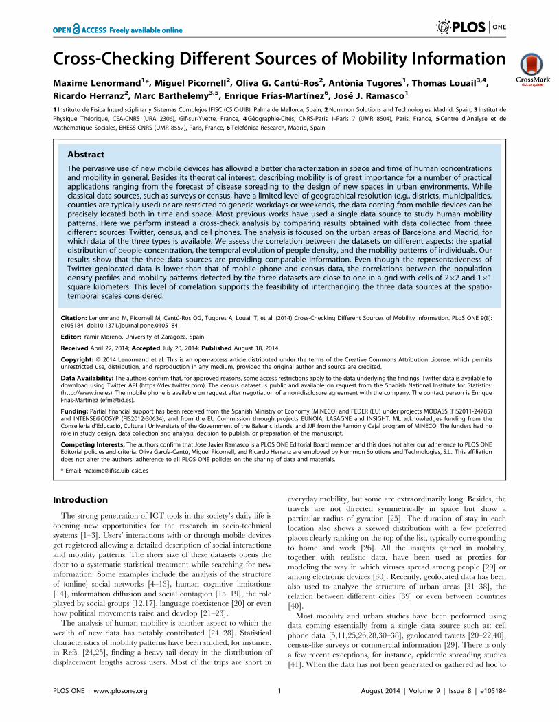
area covered by each tower can be approximated by a Voronoi

tessellation of the urban areas, as shown in Figure 1a for

Barcelona. Each call originated or received by a user and served

by a BTS is thus assigned to the corresponding BTS Voronoi area.

In order to estimate the number of people in different areas per

period of time, we use the following criteria: each person counts

only once per hour. If a user is detected in k different positions

within a certain 1-hour time period, each registered position will

count as (1/k) ‘‘units of activity’’. From such aggregated data,

activity per zone and per hour is calculated. Consider a generic

grid cell g for a day d and hour between h and h+1, the m Voronoi

areas intersecting g are found and the number of mobile phone

users Pg,d,h is calculated as follows:

Pg,d,h~Xm

v~1

Nv,d,hAv\g

Av

, ð1Þ

where Nv,d,h is the number of users in a Voronoi cell v on day d at

time h, Av\g is the area of the intersection between v and g, and

Av the area of v. The D days available in the database are then

divided in four groups according to the classification explained

above and the average number of mobile phone users for each day

group w is computed as

Pg,w,h~

Pd[Dw

Pg,d,h

DDwD: ð2Þ

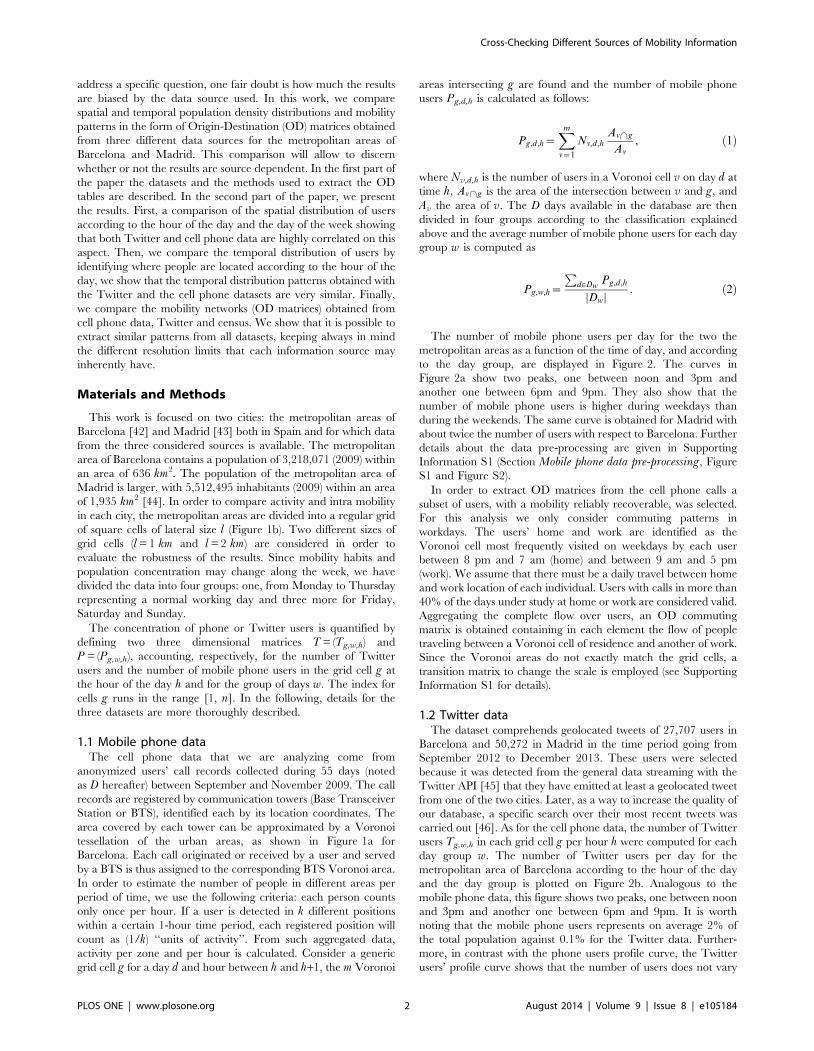
The number of mobile phone users per day for the two the

metropolitan areas as a function of the time of day, and according

to the day group, are displayed in Figure 2. The curves in

Figure 2a show two peaks, one between noon and 3pm and

another one between 6pm and 9pm. They also show that the

number of mobile phone users is higher during weekdays than

during the weekends. The same curve is obtained for Madrid with

about twice the number of users with respect to Barcelona. Further

details about the data pre-processing are given in Supporting

Information S1 (Section Mobile phone data pre-processing, Figure

S1 and Figure S2).

In order to extract OD matrices from the cell phone calls a

subset of users, with a mobility reliably recoverable, was selected.

For this analysis we only consider commuting patterns in

workdays. The users’ home and work are identified as the

Voronoi cell most frequently visited on weekdays by each user

between 8 pm and 7 am (home) and between 9 am and 5 pm

(work). We assume that there must be a daily travel between home

and work location of each individual. Users with calls in more than

40% of the days under study at home or work are considered valid.

Aggregating the complete flow over users, an OD commuting

matrix is obtained containing in each element the flow of people

traveling between a Voronoi cell of residence and another of work.

Since the Voronoi areas do not exactly match the grid cells, a

transition matrix to change the scale is employed (see Supporting

Information S1 for details).

1.2 Twitter dataThe dataset comprehends geolocated tweets of 27,707 users in

Barcelona and 50,272 in Madrid in the time period going from

September 2012 to December 2013. These users were selected

because it was detected from the general data streaming with the

Twitter API [45] that they have emitted at least a geolocated tweet

from one of the two cities. Later, as a way to increase the quality of

our database, a specific search over their most recent tweets was

carried out [46]. As for the cell phone data, the number of Twitter

users Tg,w,h in each grid cell g per hour h were computed for each

day group w. The number of Twitter users per day for the

metropolitan area of Barcelona according to the hour of the day

and the day group is plotted on Figure 2b. Analogous to the

mobile phone data, this figure shows two peaks, one between noon

and 3pm and another one between 6pm and 9pm. It is worth

noting that the mobile phone users represents on average 2% of

the total population against 0.1% for the Twitter data. Further-

more, in contrast with the phone users profile curve, the Twitter

users’ profile curve shows that the number of users does not vary

Cross-Checking Different Sources of Mobility Information


much from weekdays to weekend days. Moreover, we can observe

that the number of Twitter users is higher during the second peak

than during the first one.

The identification of the OD commuting matrices using Twitter

is similar to the one explained for the mobile phones except for

two aspects. Since the number of geolocated tweets is much lower

than the equivalent in calls per user, the threshold for considering

a user valid is set at 100 tweets on weekdays in all the dataset. The

other difference is that since the tweets are geolocated with latitude

and longitude coordinates, the assignment to the grid cells is done

Figure 1. Map of the metropolitan area of Barcelona. The white area represents the metropolitan area, the dark grey zones correspond toterritory surrounding the metropolitan area and the gray zones to the sea. (a) Voronoi cells around the BTSs. (b) Gird cells of size 262 km2.doi:10.1371/journal.pone.0105184.g001

Figure 2. Number of mobile phone users per day in Barcelona (a) and Madrid (c) and number of Twitter users in Barcelona (b) andMadrid (d) as a function of the time according to day group w. From left to right: weekdays (aggregation from Monday to Thursday), Friday,Saturday and Sunday.doi:10.1371/journal.pone.0105184.g002



directly without the need of intermediate steps through the

Voronoi cells. As for the phone, we keep only users working and

living within the metropolitan areas.

1.3 Census dataThe Spanish census survey of 2011 included a question referring

to the municipality of work of each interviewed individual. This

survey has been conducted among one fifth of the population. This

information, along with the municipality of the household where

the interview was carried out, allows for the definition of OD flow

matrices at the municipal level [44]. For privacy reasons, flows

with a number of commuters lower than 10 have been removed.

The metropolitan area of Barcelona is composed of 36 munici-

palities, while the one of Madrid contains 27 municipalities. In

addition to the flows, we have obtained the GIS files with the

border of each municipality from the census office. This

information is used to map the OD matrices from Twitter or

the cell phone data to this more coarse-grained spatial scale to

compare mobility patterns across datasets.

1.4 Ethics statementThis work includes the use of users’ geolocated information.

Since we are interested only in statistical features and not in

individual traits of users, all the data have been anonymized and

aggregated before the analysis that has been performed in

accordance with all local data protection laws. Twitter and Census

data are obtained from public sources as explained above. The cell

phone data is proprietary and subject to strict privacy regulations.

The access to this dataset was granted after reaching a non

disclosure agreement with the proprietary, who anonymized and

aggregated the original data before giving access to other authors.

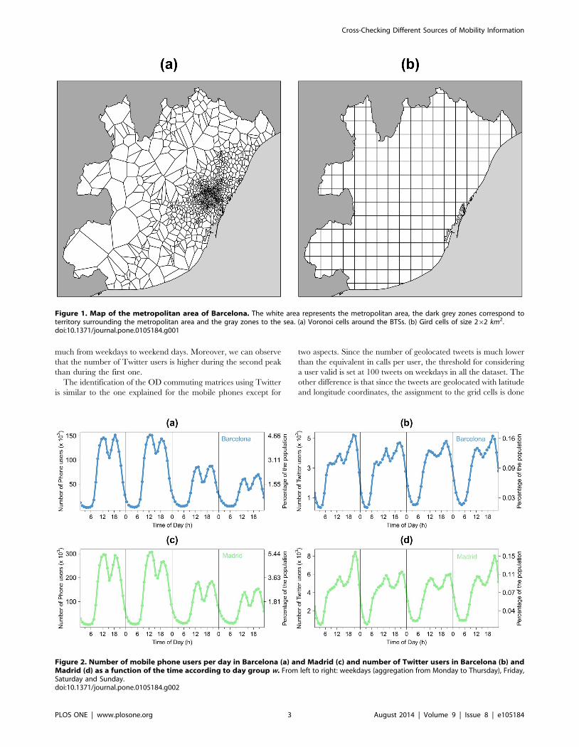
Figure 3. Correlation between the spatial distribution of Twitter users and mobile phone users for the weekdays (aggregation fromMonday to Thursday) and from noon to 1pm for the metropolitan area of Barcelona (l = 2 km). (a) Scatter-plot composed by each pair(Tg,w,h, Pg,w,h), the values have been normalized (dividing by the total number of users) in order to obtain values between 0 and 1. The red linerepresents the perfect linear fit with slope equal to 1 and intercept equal to 0. ((b)–(c)) Spatial distribution of Twitter users (b) and mobile phone users(c). In order to facilitate the comparison of both distributions on the map, the proportion of users in each cell is shown (always bounded in theinterval [0, 1]).doi:10.1371/journal.pone.0105184.g003

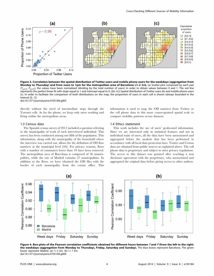
Figure 4. Box-plots of the Pearson correlation coefficients obtained for different hours between T and P (from the left to the right:the weekdays (aggregation from Monday to Thursday), Friday, Saturday and Sunday). The blue boxes represent Barcelona. The greenboxes represent Madrid. (a) l = 2 km. (b) l = 1 km.doi:10.1371/journal.pone.0105184.g004



Results

2.1 Spatial distributionA first question to address is how much the human activity level

is similar or not when estimated from Twitter, T, or from cell

phone data P across the urban space in grid cells of 2 by 2 km. To

quantify similarity, we start by depicting in Figure 3 a scatter plot

composed by each pair (Tg,w,h, Pg,w,h) for every grid cell of the

metropolitan area of Barcelona taking w as the weekdays

(aggregation from Monday to Thursday). The hour h is set from

midday to 1pm. A first visual inspection tells us that the agreement

between the activity inferred from each dataset is quite good. In

fact, the Pearson correlation coefficient between the two estimators

of activity is of r~0:96. Furthermore, the portion of activity can

Figure 5. Temporal distribution patterns for the metropolitan area of Barcelona (l = 2 km). (a), (c) and (e) Mobile phone activity; (b), (d)and (f) Twitter activity; (a) and (b) Business cluster; (c) and (d) Residential/leisure cluster; (e) and (f) Nightlife cluster.doi:10.1371/journal.pone.0105184.g005



be depicted on two maps as in Figure 3b and c. The similarity of

the areas of concentration of the activity is patent.

More systematically, we plot in Figure 4a, the box-plots of the

Pearson correlation coefficients for each day group and both case

studies as observed for different hours. We obtain in average a

correlation of 0.93 for Barcelona and 0.89 for Madrid. Globally,

the correlation coefficients have higher value for Barcelona than

for Madrid probably because the metropolitan area of Madrid is

about four times larger than the one of Barcelona. It is interesting

to note that the average correlation remains high even if we

increase the resolution by using a value of l equal to 1 km. Indeed,

we obtain in average a correlation of 0.85 for Barcelona and 0.83

for Madrid at that new scale (Figure 4b).

2.2 Temporal distributionAfter the spatial distribution of activity, we investigate the

correlation between the temporal activity patterns as observed

from each grid cell. We start by normalizing T and P such that the

total number of users at a given time on a given day is equal to 1

TTg0,w,h~Tg0,w,hPng~1 Tg,w,h

, ð3Þ

PPg0,w,h~Pg0,w,hPng~1 Pg,w,h

: ð4Þ

This normalization allows for a direct comparison between

sources with different absolute user’s activity. For a given grid cell

g~g0, we defined the temporal distribution of users PPg0as the

concatenation of the temporal distribution of users associated with

each day group. For each grid cell we obtained a temporal

distribution of users represented by a vector of length 96

corresponding to the 4624 hours.

After removing cells with zero temporal distribution, cells of

common temporal profies were found using the ascending

hierarchical clustering (AHC) method. The average linkage

clustering and the Pearson correlation coefficient were taken as

agglomeration method and similarity metric, respectively [47]. We

have also implemented the k-means algorithm for extracting

clusters but better silhouette index values were obtained with the

AHC algorithm (see details in Figure S3 in Supporting Informa-

tion S1). To choose the number of clusters, we used the average

silhouette index �SS [48]. For each cell g, we can compute a(g) the

average dissimilarity of g (based on the Pearson correlation

coefficient in our case) with all the other cells in the cluster to

which g belongs. In the same way, we can compute the average

dissimilarities of g to the other clusters and define b(g) as the lowest

average dissimilarity among them. Using these two quantities, we

compute the silhouette index s(g) defined as

s(g)~b(g){a(g)

maxfa(g),b(g)g , ð5Þ

which measures how well clustered g is. This measure is comprised

between 21 for a very poor clustering quality and 1 for an

appropriately clustered g. We choose the number of clusters that

maximize the average silhouette index over all the grid cells

�SS~Pn

g~1 s(g).

n.

For the mobile phone data, three clusters were found with an

average silhouette index equal to 0.38 for Barcelona and to 0.43

Figure 6. Comparison between the non-zero flows obtained with the Twitter dataset and the mobile phone dataset (the valueshave been normalized by the total number of commuters for both OD tables). The points are scatter plot for each pair of grid cells. The redline represents the x = y line. (a) Barcelona. (b) Madrid. In both cases l = 2 km.doi:10.1371/journal.pone.0105184.g006



for Madrid. The three temporal distribution patterns of mobile

phone users are shown in Figure 5 for Barcelona. These three

clusters can be associated with the following land uses:

N Business: this cluster is characterized by a higher activity

during the weekdays than the weekend days. In Figure 5a, we

observe that the activity takes place between 6 am and 3 pm

with a higher activity during the morning.

N Residential: this cluster is characterized by a higher activity

during the weekend days than during the weekdays. Figure 5c

shows that the activity is almost constant from 9 am during the

weekend days. During the weekdays we observe two peaks, the

first one between 7 am and 8 am and the second one during

the evening.

N Nightlife: this cluster is characterized by a high activity

during the night especially the weekend (Figure 5e).

It is remarkable to note that we obtain the same three patterns

for Madrid and that these patterns are robust for different values of

the scale parameter l (see details in Figure S4, S5 and S6 in

Supporting Information S1).

For Twitter data, considering a number of clusters smaller than

10, silhouette index values lower than 0.1 are obtained for both

case studies. These low values mean that no clusters have been

detected in the data probably because the Twitter data are too

noisy. A way to bypass this limitation is to check if, for both data

sources, the same patterns are obtained considering the different

clusters obtained with the mobile phone data. To do so the

temporal distribution patterns of Twitter users associated with the

three clusters obtained with the mobile phone data are computed.

We note in Figure 5 that for Barcelona the temporal distribution

patterns obtained with the Twitter data are very similar to those

obtained with the mobile phone data. We obtain the same

correlation for Madrid and for different values of the scale l (see

details in Figure S4, S5 and S6 in Supporting Information S1).

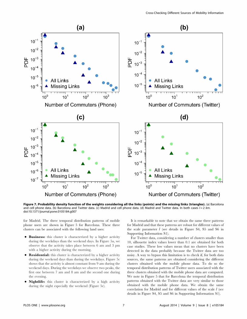
Figure 7. Probability density function of the weights considering all the links (points) and the missing links (triangles). (a) Barcelonaand cell phone data. (b) Barcelona and Twitter data. (c) Madrid and cell phone data. (d) Madrid and Twitter data. In both cases l = 2 km.doi:10.1371/journal.pone.0105184.g007



2.3 Users’ mobilityIn this section, we study the similarity between the OD matrices

extracted from Twitter and cell phone data. As it involves a

change of spatial resolution needing extra attention, the compar-

ison with the census is relegated to a coming section. We are able

to infer for the metropolitan areas of Barcelona and Madrid the

number of individuals living in the cell i and working in the cell j.Figure 6 shows a scattered plot with the comparison between the

flows obtained in the OD matrices for links present in both

networks. In order to compare the two networks, the values have

been normalized by the total number of commuters.

The overall agreement is good, the Pearson correlation

coefficient is around r&0:9. This coefficient measures the strength

of the linear relationship between the normalized flows extracted

from both networks, including the zero flows (i.e. flows with zero

commuters). However, a high correlation value is not sufficient to

assess the goodness of fit. Since we are estimating the fraction of

commuters on each link, the values obtained from Twitter and the

cell phone data should be ideally not only linearly related but the

same. That is, if y if the estimated fraction of mobile phone users

on a connection and x the estimated Twitter users on the same

link, there should be not only a linear relation, which involves a

high Pearson correlation, but also y = x. It is, therefore, important

to verify that the slope of the relationship is equal to one. To do so,

the coefficients of determination R2 are computed to measure how

well the scatterplot if fitted by the curve y = x. Since there is no

particular preference for any set of data as x or y, two coefficients

R2 can be measured, one using Twitter data as the independent

Figure 8. Commuting distance distribution obtained with both datasets. We only consider individuals living and working in two differentgrid cells. The circles represent the Twitter data and the triangles the mobile phone data. (a) Barcelona. (b) Madrid. In both cases l = 2 km.doi:10.1371/journal.pone.0105184.g008

Figure 9. Comparison between the non-zero flows obtained with the three datasets for the Barcelona’s case study (the values havebeen normalized by the total number of commuters for both OD tables). Blue points are scatter plot for each pair of municipalities. The redline represents the x = y line. (a) Twitter and mobile phone. (b) Census and mobile phone. (c) Census and Twitter.doi:10.1371/journal.pone.0105184.g009



variable x and another using cell phone data. Note that if the slope

of the relationship is strictly equal to one the two R2 must be equal

to the square of the correlation coefficient, we obtain a value

around R2 = 0.85 for Barcelona and around 0.81 for Madrid. The

slope of the best fit is in both cases very close to one.

The dispersion in the points is higher in low flow links. This can

be explained by the stronger role played by the statistical

fluctuations in low traffic numbers. Moreover, if we increase the

resolution by using a value of l equal to 1 km, the Pearson

correlation coefficient remains high with a value around 0.8 (see

details in Figure S7 in Supporting Information S1). The extreme

situation of these fluctuations occurs when a link is present in one

network and it has zero flow in the other (missing links). On

average 90% of these links have a number of commuters equal to

one in the network in which they are present. This shows that the

two networks are not only inferring the same mobility patterns, but

that the information left outside in the cross-check corresponds to

the weakest links in the system. In order to assess the relevance of

the missing links, the weight distributions of these links is displayed

in Figure 7 for all the networks and case studies. As a comparison

line, the weight distribution of all the links are also shown in the

different panels. In all cases, the missing links have flows at least

one order of magnitude, sometimes two orders, lower than the

strongest links in the corresponding networks. To be more precise,

the strongest flow of the missing links is, depending on the case,

between 25 and 464 times lower than the highest weight of all the

links. Furthermore, the average weight of the missing links is

between 4 and 9 times lower than that obtained over all the links.

Most of the missing links are therefore negligible in the general

network picture.

With the aim of going a little further, we analyze and compare

next the distance distribution for the trips obtained from both

datasets. The geographical distance along each link in the OD

matrices is calculated and the number of people traveling in the

links is taken into account to evaluate the travel-length distribu-

tion. Figure 8 shows these distributions for each network. Strong

similarity between the two distributions can be observed in the two

cities considered.

2.4 Census, Twitter and cell phoneAs a final cross-validation, we compare the OD matrices

estimated in workdays from Twitter and cell phone data to those

extracted from the 2011 census in Barcelona and Madrid. The

census data is at the municipal level, which implies that to be able

to perform the comparative analysis the geographical scale of both

Twitter and phone data must be modified. To this end, the GIS

files with the border of each municipality were used, instead of the

grid, to compute the OD matrices from Twitter and cell phone

data. Figure 9 shows a scattered plot with the comparison between

the flows obtained with the three networks. A good agreement

between the three datasets is obtained with a Pearson correlation

coefficient around r&0:99. As mentioned previously, the corre-

lation coefficient is not sufficient to assess the goodness of fit

between the two networks. Thus, we have also computed two

coefficients of determination R2 for each one of the three

relationships to measure how well the line x = y approximates

the scatter plots. For the two first relationships, the comparison

between the Twitter and the mobile phone and the comparison

between the mobile phone and the census OD tables, we obtain

R2 values higher than 0.95. For the last relationship (Twitter vs

census), two different R2 values are obtained because the best fit

slope of the scatter plot is not strictly equal to one (0.85). The first

R2 value, which measure how well the normalized flows obtained

in the Twitter’s OD matrix approximate the normalized flows

obtained in the census’s OD matrix, is equal to 0.8 and the second

value, which assess the quality of the opposite relationship, is equal

to 0.9. A better result is instead obtained for Madrid with a

Pearson correlation coefficient around 0.99 and coefficients of

determination higher than 0.97 (see details in Figure S8 in

Supporting Information S1).

Discussion

In summary, we have analyzed mobility in urban areas

extracted from different sources: cell phones, Twitter and census.

The nature of the three data sources is very different, as also is the

resolution scales in which the mobility information is recovered.

For this reason, the aim of this work has been to run a thorough

comparison between the information collected at different spatial

and temporal scales. The first aspect considered refers to the

population concentration in different parts of the cities. This point

is of great importance in the analysis and planning of urban

environments, including the design of new services or of

contingency plans in case of disasters. Our results show that both

Twitter and cell phone data produce similar density patterns both

in space and time, with a Pearson correlation close to 0.9 in the

two cities analyzed. The second aspect considered has been the

temporal distribution of individuals which allow us to determine

the type of activity that are most common in specific urban areas.

We show that similar temporal distribution patterns can be

extracted from both Twitter and cell phone datasets. The last

question studied has been the extraction of mobility networks in

the shape of Origin-Destination commuting matrices. We observe

that at high spatial resolution, in grid cells with sides of 1 or 2 km,

the networks obtained with both cell phones and Twitter are

comparable. Of course, the integration time needed for Twitter is

higher in order to obtain similar results. Twitter data can run in

serious problems too if instead of recurrent mobility the focus is on

shorter term mobility, but this point falls beyond the scope of this

work. Finally, the comparison with census data is also acceptable:

both Twitter and cell phone data reproduce the commuting

networks at the municipal scale from an overall perspective. Still

and although good on average, the agreement between the three

different datasets is broken in some particular connections that

deviate from the diagonal in our scatterplots. This can be

explained by the fact that the datasets come from different

sources, were collected in different years and may have different

biases and level of representativeness. For example, Twitter is

supposed to be used more by younger people. The explanation of

these deviations and whether they are just stochastic fluctuations

or follow some rationale could be an interesting avenue for further

research.

These results set a basis for the reliability of previous works

basing their analysis on single datasets. Similarly, the door to

extract conclusions from data coming from a single data source

(due to convenience of facility of access) is open as long as the

spatio-temporal scales tested here are respected.

Supporting Information

Supporting Information S1 Supporting files and figures.(PDF)

Author Contributions

Conceived and designed the experiments: ML JJR OGC MP. Performed

the experiments: ML JJR OGC MP. Analyzed the data: ML JJR OGC

MP. Contributed reagents/materials/analysis tools: ML JJR OGC MP AT

RH EFM TL MB. Contributed to the writing of the manuscript: ML JJR

OGC MP AT RH EFM TL MB.



References

1. Watts DJ (2007) A twenty-first century science. Nature 445: 489.

2. Lazer D, Pentland A, Adamic L, Aral S, Barabasi AL, et al. (2009)Computational social science. Science 323: 721.

3. Vespignani A (2009) Predicting the behavior of techno-social systems. Science325: 425–428.

4. Liben-Nowell D, Novak J, Kumar R, Raghavan P, Tomkins A (2005)

Geographic routing in social networks. Proc Natl Acad Sci USA 102: 11623–11628.

5. Onnela JP, Saramaki J, Hyvonen J, Szabo G, Lazer D, et al. (2007) Structureand tie strengths in mobile communication networks. Proc Natl Acad Sci USA

104: 7332–7336.

6. Java A, Song X, Finin T, Tseng B (2007) Why we Twitter: understandingmicroblogging usage and communities. Proc. 9th WEBKDD and 1st SNA-KDD

2007.7. Huberman BA, Romero DM, Wu F (2008) Social networks that matter: Twitter

under the microscope. First Monday 14.8. Krishnamurthy B, Gill P, Arlitt M (2008) A few chirps about Twitter. Proc.

WOSP’08.

9. Lewis K, Kaufman J, Gonzalez M, Wimmer A, Chirstakis N (2008) Tastes, tiesand time: a new social network dataset using Facebook.com. Social Networks 30:

330–342.10. Mislove A, Koppula HS, Gummadi KP, Druschel P, Bhattacharjee B (2008)

Growth of the flickr social network. Proceedings of the first workshop on Online

Social Networks – WOSP’08. pp. 25–30.11. Eagle N, Pentland AS, Lazer D (2009) From the Cover: Inferring friendship

network structure by using mobile phone data. Proc Natl Acad Sci USA 106:15274–15278.

12. Ferrara E (2012) A large-scale community structure analysis in Facebook. EPJData Science 1: 9.

13. Grabowicz PA, Ramasco JJ, Goncalves B, Eguiluz VM (2013) Entangling

mobility and interactions in social media. ArXiv e-print arXiv:1307.5304.14. Goncalves B, Perra N, Vespignani A (2011) Modeling users’ activity on twitter

networks: Validation of Dunbar’s number. PLoS ONE 6: e22656.15. Leskovec J, Backstrom L, Kleinberg J (2009) Meme-tracking and the dynamics

of the news cycle. Proceedings of the 15th ACM SIGKDD international

conference on knowledge discovery and data mining – KDD’09, p. 497–506.16. Lehmann J, Goncalves B, Ramasco JJ, Cattuto C (2012) Dynamical classes of

collective attention in Twitter. Proceedings of the 21st international conferenceon World Wide Web – WWW’12. p. 251–260.

17. Grabowicz PA, Ramasco JJ, Moro E, Pujol JM, Eguıluz VM (2012) Socialfeatures of online networks: the strength of intermediary ties in online social

media. PLoS ONE 7: e29358.

18. Bakshy E, Rosenn I, Marlow C, Adamic L (2012) The role of social networks ininformation diffusion. Proceedings of the 21st international conference on World

Wide Web – WWW’12, pp. 519–528.19. Ugander J, Backstrom L, Marlow C, Kleinberg J (2012) Structural diversity in

social contagion. Proc Natl Acad Sci USA 109: 5962–5966.

20. Mocanu D, Baronchelli A, Perra N, Gonalves B, Zhang Q, et al. (2013) TheTwitter of Babel: Mapping World Languages through Microblogging Platforms.

PLoS ONE 8: e61981.21. Borge-Holthoefer J, Rivero A, Garcıa IN, Cauhe E, Ferrer A, et al. (2011)

Structural and dynamical patterns on online social networks: The Spanish may15th movement as a case study. PLoS ONE 6: e23883.

22. Gonzalez-Bailon M, Borge-Holthoefer J, Rivero A, Moreno Y (2011) The

dynamics of protest recruitment through an online network. Scientific Reports 1:197.

23. Conover MD, Davis C, Ferrara E, McKelvey K, Menczer F, et al. (2013) Thegeospatial characteristics of a social movement communication network. PLoS

ONE 8: e55957.

24. Brockmann D, Hufnagel L, Geisel T (2006) The scaling laws of human travel.Nature 439: 462–465.

25. Gonzalez MC, Hidalgo CA, Barabasi AL (2008) Understanding individual

human mobility patterns. Nature 453: 779–782.

26. Song C, Qu Z, Blumm N, Barabasi AL (2010) Limits of predictability in human

mobility. Science 327: 1018–1021.

27. Bagrow JP, Lin YR (2012) Mesoscopic structure and social aspects of human

mobility. PLoS ONE 7: e37676.

28. Phithakkitnukoon S, Smoreda Z, Olivier P (2012) Socio-geography of humanmobility: A study using longitudinal mobile phone data. PLoS ONE 7: e39253.

29. Balcan D, Colizza V, Goncalves B, Hu H, Ramasco JJ, et al. (2009) Multiscalemobility networks and the spatial spreading of infectious diseases. Proc Natl

Acad Sci USA 106: 21484–21489.

30. Wang P, Gonzalez MC, Hidalgo CA, Barabsi AL (2009) Understanding the

spreading patterns of mobile phone viruses. Science 324: 1071–1076.

31. Ratti C, Pulselli RM, Williams S, Frenchman D (2006) Mobile landscapes: usinglocation data from cell phones for urban analysis. Environment and Planning B:

Planning and Design 33: 727–748.

32. Reades J, Calabrese F, Sevtsuk A, Ratti C (2007) Cellular census: Explorations in

urban data collection. Pervasive Computing, IEEE 6: 30–38.

33. Soto V, Frıas-Martınez E (2011) Robust land use characterization of urban

landscapes using cell phone data. In: Proceedings of the 1st Workshop on

Pervasive Urban Applications, in conjunction with 9th Int. Conf. PervasiveComputing

34. Frıas-Martınez V, Soto V, Hohwald H, Frıas-Martınez E (2012) Characterizingurban landscapes using geolocated tweets. In: SocialCom/PASSAT. IEEE, pp.

239–248.

35. Isaacman S, Becker R, Caceres R, Martonosi M, Rowland J, et al. (2012)

Human mobility modeling at metropolitan scales. In: Proceedings of the

International Conference on Mobile Systems, Applications, and Services(MobiSys). ACM, pp. 239–252.

36. Toole JL, Ulm M, Bauer D, Gonzalez MC (2012) Inferring land use from mobilephone activity. In: ACM UrbComp2012.

37. Pei T, Sobolevsky S, Ratti C, Shaw SL, Zhou C (2013) A new insight into land

use classification based on aggregated mobile phone data. ArXiv e-print arxiv:1310.6129.

38. Louail T, Lenormand M, Garcia Cantu O, Picornell M, Herranz R, et al. (2014)From mobile phone data to the spatial structure of cities. ArXiv e-print

arxiv:1401.4540.

39. Noulas A, Scellato S, Lambiotte R, Pontil M, Mascolo C (2012) A tale of many

cities: Universal patterns in human urban mobility. PloS ONE 7: e37027.

40. Hawelka B, Sitko I, Beinat E, Sobolevsky S, Kazakopoulos P, et al. (2013) Geo-located twitter as a proxy for global mobility patterns. ArXiv e-print

arXiv:1311.0680.

41. Tizzoni M, Bajardi P, Decuyper A, Kon Kam King G, Schneider CM, et al.

(2013) On the use of human mobility proxy for the modeling of epidemics.ArXiv e-print arXiv:1309.7272.

42. Area Metropolitana de Barcelona (nd) Metropolitan Area of Barcelona.

Available: http://www.amb.cat. Accessed 2014 July 23.

43. Community of Madrid (nd) see ‘‘Atlas de la Comunidad de Madrid en el siglo

XXI’’.

44. Instituto Nacional de Estadıstica (National Institute for Statistics) (2014) Instituto

Nacional de Estadıstica. Available: http://www.ine.es. Accessed 2014 July 23.

45. Twitter API (nd) section for developers of Twitter Web page. Available: https://dev.twitter.com. Accessed 2014 July 23.

46. Tugores A, Colet P (2013) Big data and urban mobility, Proceedings of the 7thIberian Grid infraestructure conference.

47. Hastie T, Tibshirani R, Friedman J (2009) The elements of statistical learning(2nd ed.). New York: Springer-Verlag.

48. Rousseeuw PJ (1987) Silhouettes: A graphical aid to the interpretation and

validation of cluster analysis. Journal of Computational and Applied Mathe-matics 20: 53–65.



http://www.amb.cat

http://www.ine.es



cross-checking different sources of mobility...

Documents