criterion-related validity – predictive lecture 10 epsy 625

CRITERION-RELATED VALIDITY – PREDICTIVE

LECTURE 10

EPSY 625

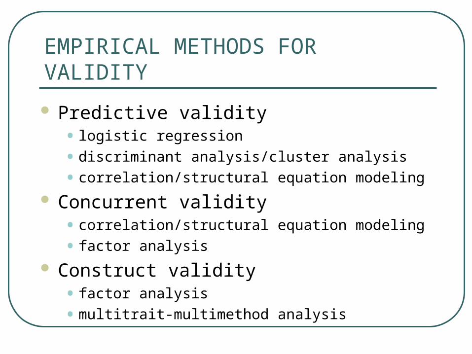
EMPIRICAL METHODS FOR VALIDITY

Predictive validity• logistic regression

• discriminant analysis/cluster analysis

• correlation/structural equation modeling

Concurrent validity• correlation/structural equation modeling

• factor analysis

Construct validity• factor analysis

• multitrait-multimethod analysis

PREDICTIVE VALIDITY- logistic regression

Binary group: (0,1) such as hired vs. not hired, general vs. clinical

Transform binary score into logit:

L(y) = log[p/(1-p)]

Predict L(y) = b1 x, where x is a test score

Can use SPSS LOGISTIC option in REGRESSION analysis

Omnibus Tests of Model Coefficients

83.360 14 .000

83.360 14 .000

83.360 14 .000

Step

Block

Model

Step 1Chi-square df Sig.

Model Summary

292.234a .265 .353Step1

-2 Loglikelihood

Cox & SnellR Square

NagelkerkeR Square

Estimation terminated at iteration number 4 becauseparameter estimates changed by less than .001.

a.

Classification Tablea

101 32 75.9

35 103 74.6

75.3

Observed0

1

clinical

Overall Percentage

Step 10 1

clinical PercentageCorrect

Predicted

The cut value is .500a.

Variables in the Equation

-.069 .024 8.374 1 .004 .933

.051 .021 5.854 1 .016 1.052

.004 .016 .059 1 .809 1.004

.026 .017 2.297 1 .130 1.027

.051 .019 7.404 1 .007 1.052

-.046 .028 2.683 1 .101 .955

-.047 .017 7.897 1 .005 .954

-.004 .019 .041 1 .840 .996

-.022 .021 1.101 1 .294 .978

.044 .023 3.793 1 .051 1.045

-.005 .025 .046 1 .829 .995

-.027 .017 2.542 1 .111 .973

.045 .022 4.083 1 .043 1.046

.047 .024 3.843 1 .050 1.048

-2.668 2.529 1.113 1 .291 .069

t1

t10

t11

t12

t13

t14

t2

t3

t4

t5

t6

t7

t8

t9

Constant

Step1

a

B S.E. Wald df Sig. Exp(B)

Variable(s) entered on step 1: t1, t10, t11, t12, t13, t14, t2, t3, t4, t5, t6, t7, t8, t9.a.

VARIABLE LABELSt1 ANXIETYt2 ATTITUDE TO PARENTSt3 ATTITUDE TO SCHOOLt4 ATTITUDE TO TEACHERt5 ATYPICALITYt6 DEPRESSIONt7 INTERPERSONAL RELATIONSt8 SENSE OF INADEQUACYt9 LOCUS OF CONTROLt10SELF ESTEEMt11SELF RELIANCEt12SENSATION SEEKINGt13SOMATICIZATIONt14 SOCIAL STRESS

Multinomial regression

Extension of logistic regression 3 or more groups contrasted

• Ordered groups- compute “threshhold for classification as a “1” or “2” , “2” or “3” etc

• Unordered groups- can do pairwise logistic regression or a priori contrasts among groups as the organizer for binomial contrasting (eg. groups A and B vs. groups C, D, and E)

PREDICTIVE VALIDITY – DISCRIMINANT ANALYSIS

Test scores Group membership

eg, which MMPI scales differentiate/separate/predict manic depressives from normal functioning adults? This will be useful upon intake or commitment hearings in addition to clinical judgement

DISCRIMINANT ANALYSIS

2 Groups: statistical procedure is identical to multiple regression with group (1 or 2) as dependent variable, k test scores as predictors

3 or more Groups: discriminant analysis separates the groups based on a weighted sum of the predictors in standardized form

2 Group Analysis

Model:y = b1x1 + b2x2 + …bkxk + b0

y = 1 or 2 (or any two discrete numbers)

creates single predicted score Dhat which is the predicted score for each person. Can compare this predicted score with actual diagnoses or condition to determine % hit rate

2 Group Analysis

y2

y1

Group 1

means

Group 2

means

D=b1y1+b2y2

R2 = SSD / SStot

2 Group hit rate

Example: predict male (1) vs. female (2) differences based on interests x1, x2, … xk

Each person receives a score yhat ; if yhat is below 1.5 the person is predicted to be a male, if over 1.5, a female.

Out of 100 persons (50 M, 50 F), by chance we would classify 50 correctly by chance;

2 Group hit rate

Cohen’s kappa will provide evidence for correct classification beyond chance:

k = Pc - P0/[1 - P0]

Alternatively, R2 for the regression provides evidence for classification beyond chance.

Coefficientsa

1.531 .049 31.415 .000

3.476E-03 .012 .008 .283 .777

-4.29E-03 .016 -.009 -.275 .784

1.492E-02 .015 .033 1.017 .309

(Constant)

Country Western Music

Blues or R & B Music

Jazz Music

Model1

B Std. Error

UnstandardizedCoefficients

Beta

Standardized

Coefficients

t Sig.

Dependent Variable: Respondent's Sexa.

ANOVAb

.291 3 9.714E-02 .395 .757a

344.415 1400 .246

344.707 1403

Regression

Residual

Total

Model1

Sum ofSquares df

MeanSquare F Sig.

Predictors: (Constant), Jazz Music, Country Western Music, Blues or R & B Musica.

Dependent Variable: Respondent's Sexb.

Example: Gender predicted from music preferences

R2 = SSb / SStot = .291/344.7 = .001

Descriptive Statistics

1500 1.57 .49 1 2

1404 1.3967 .4894 1.00 2.00

Respondent's Sex

SEXHAT

N MeanStd.

Deviation Minimum Maximum

Respondent's Sex * SEXHAT Crosstabulation

Count

382 226 608

465 331 796

847 557 1404

Male

Female

Respondent'sSex

Total

1.00 2.00

SEXHAT

Total

Symmetric Measures

.045 .094

.042 .025 1.674 .094

1404

Contingency CoefficientNominal by Nominal

KappaMeasure of Agreement

N of Valid Cases

ValueAsymp.

Std. Errora

Approx. Tb

Approx.Sig.

Not assuming the null hypothesis.a.

Using the asymptotic standard error assuming the null hypothesis.b.

Discriminant Analysis

Eigenvalues

.001a 100.0 100.0 .029Function1

Eigenvalue% of

VarianceCumulative

%CanonicalCorrelation

First 1 canonical discriminant functions were used in theanalysis.

a.

Wilks' Lambda

.999 1.185 3 .757Test of Function(s)1

Wilks'Lambda Chi-square df Sig.

Wilks lambda = 1-R2

Standardized Canonical Discriminant Function Coefficients

.263

1.139

-.306


Jazz Music


1

Function

Canonical Discriminant Function Coefficients

.241

1.035

-.298

-2.507


Jazz Music


(Constant)

1

Function

Unstandardized coefficients

Functions at Group Centroids

-3.33E-02

2.540E-02

Respondent's SexMale

Female

1

Function

Unstandardized canonical discriminant functions evaluated atgroup means

males females

0.0

w

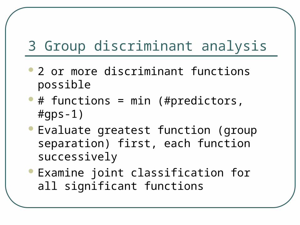
3 Group discriminant analysis

2 or more discriminant functions possible # functions = min (#predictors, #gps-1) Evaluate greatest function (group

separation) first, each function successively

Examine joint classification for all significant functions

3 Group Analysis1st discriminant function

y2

y1

Group 1

means

Group 2

means

D1=b1y1+b2y2

Group 3

means

Maximize SS between groups

3 Group Analysis2nd discriminant function

y2

y1

Group 1

means

Group 2

means

D1=b1y1+b2y2

Group 3

means

D2=b3y1+b4y2

3 Group Analysis

y2

y1

Group 1

means

Group 2

means

D1=b1y1+b2y2

R12 = SSD1 / SStot

Group 3

means

D2=b3y1+b4y2

R22 = SSD2 / SStot

3 Group Analysis

y2

y1

Group 1

means

Group 2

means

D1=b1y1+b2y2

Group 3

means

D2=b3y1+b4y2

Discriminant

function

coefficients

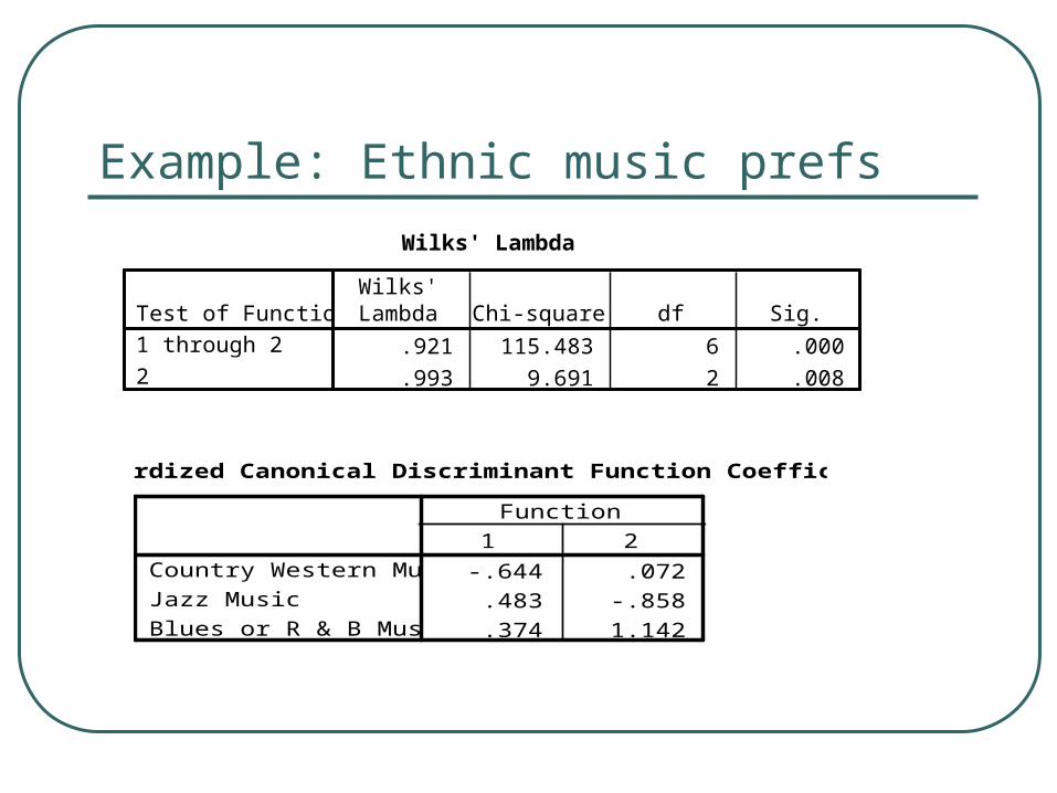
Example: Ethnic music prefsWilks' Lambda

.921 115.483 6 .000

.993 9.691 2 .008

Test of Function(s)1 through 2

2

Wilks'Lambda Chi-square df Sig.

Standardized Canonical Discriminant Function Coefficients

-.644 .072

.483 -.858

.374 1.142


Jazz Music


1 2

Function

Structure Matrix

.736* -.243

-.656* .212

.595 .680*

Jazz Music



1 2

Function

Pooled within-groups correlations between discriminatingvariables and standardized canonical discriminant functions Variables ordered by absolute size of correlation within function.

Largest absolute correlation between each variable andany discriminant function

*.

Canonical Discriminant Function Coefficients

-.599 .067

.448 -.796

.369 1.127

-.688 -.906


Jazz Music


(Constant)

1 2

Function

Unstandardized coefficients

Functions at Group Centroids

.105 -1.70E-02

-.805 -3.12E-02

-6.54E-02 .371

Racew of Respondentwhite

black

other

1 2

Function

Unstandardized canonical discriminant functions evaluated atgroup means

Territorial MapFunction 2 -3.0 -2.0 -1.0 .0 1.0 2.0 3.0 +---------+---------+---------+---------+---------+---------+ 3.0 + 21 + I 21 I I 21 I I 21 I I 21 I I 21 I 2.0 + 21 + + + + + + I 21 I I 21 I I 21 I I 21 I I 21 I 1.0 + 21 + + + + + + I 21 I I 21 I I 21 I I 21 * I I 21 I .0 + 21 + + * +* + + + I 21 I I 21 I I 21 I I 21 I I 21 I -1.0 + 21 + + + + + + I 21 I I 21 I I 21 I I 21 I I 21 I -2.0 + 21 + + + + + + I 21 I I 21 I I 21 I I 21 I I 21 I -3.0 + 21 + +---------+---------+---------+---------+---------+---------+ -3.0 -2.0 -1.0 .0 1.0 2.0 3.0 Canonical Discriminant Function 1

Symbol Group Label------ ----- --------------------

1 1 white 2 2 black 3 3 other * Indicates a group centroid

criterion-related validity – predictive lecture 10 epsy 625

Documents