1

Criminal Politicians and Firm Value: Evidence from India

Vikram Nandaa,b, Ankur Pareeka*

aRutgers Business School, Newark and New Brunswick

bUniversity of Texas at Dallas, Jindal School of Management

November 17, 2015

Abstract

Using unique datasets on the criminal background of Indian politicians and details on investment projects by Indian firms, we provide comprehensive evidence on the effects of criminal/corrupt politicians on firm value and investments. We use a regression discontinuity approach and focus on close elections to establish a causal link between the election of criminal politicians and firms’ value and investment decisions. The election of criminal politicians leads to lower election-period and project-announcement stock-market returns for private-sector firms based in the district. There is a sharp decline in the total investment by private sector firms in criminal-politician districts. Interestingly, criminal-politicians appear to offset the decline in private-sector investment by a roughly equivalent increase in investment by state-owned firms. Corrupt politicians are less destructive of value when their party is in power and when they occupy ministerial positions. JEL classification: G30; G38; D70; D72; D73 Keywords: Indian stock market; corporate investments; Political corruption; criminal politicians; rent-seeking; elections; corruption; Indian political economy

2

1. Introduction

Anecdotal and survey evidence suggest that emerging economies are rife with corruption -

- far more so than more developed economies (e.g., Svensson 2005). Contributing to the

pervasive corruption are a plethora of factors that are associated with developing

countries such as weak institutions, bureaucratic red-tape and cultural norms that are

accepting of (or resigned to) corruption. Reducing corruption has proven to be difficult –

which is not surprising since it is in the interest of beneficiaries of a corrupt system to

maintain weak institutions and complex, arbitrary rules that facilitate corruption.1

Our focus in the paper is on the rampant corruption/criminality among politicians

in India [we use corruption and criminality interchangeably in the paper]. There are

several reasons to focus on India: First, it is an important developing economy, long

plagued by corruption/criminality among its politicians and bureaucrats. In recent years

corruption has emerged as a potent political issue and affected, if not determined, the

outcome of the recent general election (2014). A second reason to focus on India is the

availability of data. The effort to clean elections in India has led to wider dissemination of

information about the background of the candidates for public office, including criminal

charges and convictions. Furthermore, there is novel and fairly comprehensive data on

project investments by Indian corporations. This enables us to investigate a number of

questions about the interplay between corruption and electoral outcomes on the one

hand -- and corporate investment decisions and investor stock market reactions on the

other.

While there are several studies of corruption in emerging economies including

India, there are relatively few reliable estimates of the actual magnitude and broader

1 An especially egregious case is that of 2-G scam in India in which rules were manipulated in arbitrary ways to favor connected bidders for spectrum licenses.

3

economic consequences of corruption. In particular, empirical evidence documenting a

link between the presence of criminal politicians and their impact on firms’ real activity

and shareholder value is limited. It is difficult to know, therefore, whether lower

corruption, at least in the context of India, could have significant implications for

economic growth. Our analysis of the data on corporate investments in the shadow of

political corruption/criminality provides some insight on the issue.

The existing literature offers mixed evidence on the relation between corruption

and economic growth. Earlier literature suggests that corruption can promote efficiency

and growth by “greasing the wheels of bureaucracy”. 2 The efficiency argument is

essentially that the most efficient firms will be assigned projects since they can afford to

pay the largest bribes. Hence, there may not be distortion in terms on allocation

outcomes.3

A sharply divergent view is the “grabbing hand” view of corruption (Shleifer and

Vishny, 1993; 1998; Frye and Shleifer, 1997). According to this view, corruption affects

economic growth. It can lead to the propping up of inefficient enterprises and a

misallocation of human and financial capital. In these environments, entrepreneurs will

seek ways to minimize their exposure to public corruption. For instance, they may adopt

inefficient “fly-by-night” technologies with a high degree of reversibility. There may be less

expropriation by corrupt officials if the entrepreneur can credibly threaten to shut down

operations (Choi and Thum, 1998; Svensson, 2003).

2 See e.g., Leff, 1964; Huntington, 1968. 3 Gorodnichenko and Peter (2007) suggests that corruption can sometimes have fairly neutral effects, They

show that, on average, public employees in Ukraine have the same consumption levels as their private sector

counterparts, even though their salaries are 24-32 percent lower. This suggests that corruption does not seem

to be providing extra income to these public employees, as what the government pays them is reduced exactly

to offset the amount they receive in bribes.

4

The evidence on the overall impact of corruption on economic growth remains

unclear, however. While corrupt environments tend to be associated with poor economic

development and growth in many instances -- there are striking counter-examples as well.

China, for instance, has been one of the most rapidly growing economies in the world, yet

corruption continues to thrive in China.

We study the effect of Indian politicians with criminal backgrounds on the value

and performance of firms and investments in their electoral districts. Since 2003, Supreme

Court of India has mandated the candidates contesting elections for federal and state

legislatures to file an affidavit declaring their pending criminal cases, past convictions,

assets, liabilities, educational qualification etc. For our study, we use a database that

collects the criminal background and other variables from the affidavits filed by candidates

with the Election Commission of India before the 2004 and 2009 General Elections for the

Lok Sabha (the lower house of Indian Parliament). We refer to these politicians as

“criminal” though, in most cases, they have been charged, rather than convicted of

criminal activity. Actual conviction rates tend to be low, possibly indicating the difficulty of

convicting politicians. The use of this data is validated by other studies that suggest that

being charged with criminal activity correlates well with other measures of corruption.4

We match the data on political candidates with that of election outcomes. This allows us

to look at the impact of criminal election victories, especially in close elections.

The literature is somewhat ambiguous as to whether the election of a criminal

politician is expected to have a negative or positive effect on the value and prospects of

firms in his/her constituency. It is plausible, for instance, that criminal politicians may

4 Banerjee and Pande (2009) estimate political corruption among candidates for political office by surveying

journalists who covered that election and politicians who stood for election in neighboring jurisdictions. They

then correlate the reported outcomes (such as whether the candidate faced criminal charges) with actual data

on the same and find a high correlation.

5

favor local firms, possibly ones that they have a past relationship with, at the expense of

non-local firms. This could be done by increasing the barriers to entry for non-local firms

through, say, making it difficult to obtain approvals for construction or utility connections.

If this occurs, firms located in criminal politicians’ districts and the projects initiated locally

by these firms could have a higher valuation compared to firms located in non-criminal

districts after controlling for other observable characteristics. An equally plausible

alternative hypothesis is that criminals are interested in maximizing their own welfare and

simply extract rents from firms located in their districts to the greatest extent they can. In

such cases, we would expect the valuation of these firms to be lower compared to firms in

non-criminal politicians’ districts.

Our data allow us to examine a number of important questions. First is whether

corrupt/criminal politicians have a meaningful impact on productive activity. We address

this by examining the value implications of new projects. To establish a causal link

between the election of criminal politicians and firm value, we use a regression

discontinuity approach commonly used in the literature on the causal effects of elections

(e.g. Lee (2008), Chemin (2012)). Specifically, we compare the effects on firm and project

values in districts where a criminal politician just won with districts where a criminal

politician just lost the election against a non-criminal candidate. Further, we examine the

response of corporations in terms of whether new investment projects are initiated and

existing ones are completed or stalled. Our overall finding is that the election of corrupt

politicians has a negative effect on firms with existing projects in the politician’s district.

Corporations are subsequently less likely to initiate or to complete projects. In addition,

the announcements of new projects are generally treated less favorably by firm investors.

6

The finding that the election of corrupt politicians appears to discourage new

investment projects and hurt the value of firms in their local areas raises the question of

how these politicians are able to get elected. We believe that the elections in India are

relatively ‘clean’ and the Election Commission in India appears to have been successful at

eliminating large-scale tampering with ballots and direct intimidation of voters. So why

then do corrupt politicians get support from voters and get elected? One explanation may

have to do with ethnic identity. It is possible that certain communities may be willing to

support politicians from their own communities (or castes) so long as the criminal

activities work in their favor or, at least, are not directed against the community. For

instance, politicians may be able to extract rent from existing enterprises and demand that

his/her supporters be favored for employment or business contracts.

It is also possible that corrupt politicians support local enterprises – while

disfavoring competition from outside firms. We, therefore, examine the impact of the

election outcomes on different types of firms: by whether firms are local vs. non-locals in

terms of their past investments and headquarter locations. And to see whether there are

differences in terms of whether the firms that are affected positively or negatively tend to

be state-majority-owned enterprises or non-state-majority owned corporations. The

notion is that a corrupt politician may have greater ability to extract rents from

enterprises in which the government is a significant owner (these are typically publicly

traded corporations that came into being as a result of partial privatization of previously

wholly-owned state corporations).

Our results indicate that both local and non-local corporations suffer when a

corrupt politician is in power. At the time of the election of a criminal politician (in close

elections) both types of firms suffer a significant loss in firm value. In terms of the market

7

reaction to the announcement of a new project investment – the negative reaction is

more evident for the non-locals. Our interpretation is that there is little surprise

associated with decisions by local firms to invest in the local area – but more of a negative

surprise when a non-local firm invests in the corrupt politician’s district. There is also a

decrease in investments by firms in the corrupt politician’s district – though the effects are

smaller for the local firms. The intriguing finding, however, is that while there is a

reduction in the investment by privately-owned corporations – this is offset to a large

extent by an increase in the investment by state-controlled enterprises – especially the

ones in which the state owns 70% or more of the voting shares. This suggests that, to an

extent, corrupt politicians may be able to keep their supporters satisfied – by providing

them employment and business opportunities with state-controlled investments over

which they may be better able to exercise control.

We also examine whether it matters as to whether the politicians are in senior

positions and/or belong to the political party that is in power at the state or national level.

Our results indicate that senior politicians (such as ministers) are not associated with

negative effect on corporations. This suggests that corrupt politicians may be more

restrained when their party is in power – and there is a stronger incentive to not disrupt

the relation between the electorate and the party. It seems that the worst outcomes are

precisely when the politician belongs to a party that is out of power – and may, therefore,

be egregiously unrestrained in terms of exercising his/her local power.

Related Literature

Our paper is related to several strands of the finance and economics literature. First, there

is a relatively new and growing literature that examines the effect of political connections

8

on firm value. Among these, Fisman (2001) studies stock market values to estimate the

value of political connections by examining the stock price reaction of Indonesian firms

connected to Suharto to news releases about his health. Faccio (2006) examines the value

of political connections in several countries and finds positive benefits channeled to

relatively poor performing firms. Similar results are reported in Goldman et al. (2007) and

Do, Lee and Nguyen (2013). Our paper also relies on the stock market values of firms that

could be affected by the election of politicians that are known to be corrupt. We find that

the election of corrupt politicians has a negative value impact on both local and non-local

investor owned firms in his/her electoral district. Investor owned firms reduce their

investments in the electoral district of corrupt politicians.

There are several papers that examine the welfare effects of criminal politicians.

For example, using data on politician affidavits, Chemin (2012) uses a regression

discontinuity (RDD) approach around elections to show that criminal politicians have a

negative effect on their constituents; in particular they reduce the consumption by the

weaker sections of the society. We rely on a similar RDD approach and examine the

impact of corruption politicians winning or losing narrowly. Fisman, Schulz and Vig (2014)

study the wealth accumulation of Indian politicians and show that annual asset growth of

election winners is 3-5% higher than losers.

Of the papers that study the impact of corruption on firm growth and investments,

Fisman and Svensson (2007) calculates bribes and tax payments in Uganda as a function of

total firm sales. They find that a 1 percentage point increase in bribes reduces annual firm

growth by three percentage points. Sequeira and Djankov (2010) examine a different type

of distortion: changes in the firm’s production choices designed to avoid corruption.

Another direct estimate of the efficiency costs due to distortion is the allocation of capital

9

from state banks. Khwaja and Mian (2005) show that politically connected firms, defined

as those with a politician on their boards, receive larger loans from government banks in

spite of having higher default rates on these loans. Our paper provides consistent

evidence of corruption-induced distortions affecting economic activity. The investments in

the districts of corrupt politicians experience a drop in new investments, especially by

non-local investor-owned firms. There is also a far higher rate of delay and stalling of

existing projects that follows the election of a corrupt politician. Hence, the election of a

criminal political has real effects in terms of the allocation/investment decisions of firms.

There is evidence that suggests that corrupt politicians favor state-owned

enterprises over non-state-controlled firms. Nguyen et al. (2012) study the relation

between corruption and growth for private firms and state-owned enterprises (SOEs) in

Vietnam. They find that corruption hampers the growth of Vietnam’s private sector, but is

not detrimental for growth in the state sector. This is consistent with our findings that

corrupt politicians appear to discourage the growth of private firms – but appear to

facilitate the growth of SOEs. An interesting finding is that the growth is experienced by

majority-state-owned firms only when the government has a greater than 70% stake in

the firm.

Finally, Shleifer and Vishny (1993) argue that centralized political institutions

provide incentives for leaders to limit the extent of arbitrary behavior on the part of

lower-level officials. When corruption is decentralized, by contrast, no individual politician

or bureaucrat fully internalizes the costs of their corrupt behavior, and property rights are

less secure as a result (Bardhan, 1997, pp. 1324–1326; Campos, Lien, & Pradhan, 1999; Li

& Lian, 2001; MacIntyre, 2001). We find support for this behavior in our study as well.

10

Corruption appears to have far worse effects when the criminal politician does not belong

to the party that is in power at the state or national level. Furthermore, senior political

leaders (such as ministers), despite having a criminal background, do not appear to have a

negative effect on investor-owned firms.

2. Data

We use data from multiple sources. Since 2003, Supreme Court of India has mandated the

candidates contesting elections for federal and state legislatures to file an affidavit

declaring their pending criminal cases, past convictions, assets, liabilities, educational

qualification etc. which allows identification of the candidates and elected members of

parliament with criminal background. The specific database we use is compiled by the

Association of Democratic Reform (available at http://www.myneta.info) that collects the

criminal background and other variables from the affidavits filed by candidates with the

Election Commission of India before the 2004 and 2009 General Elections for the Lok

Sabha or the lower house of Indian Parliament. We get the election results data i.e., the

number of votes polled for each candidate and total number of votes polled in each

constituency from the Election Commission of India website (www.eci.nic.in) and merge it

with the database of candidate background variables. We also match the parliamentary

constituencies with administrative districts using the information available on the Election

Commission of India website. Each parliamentary constituency could be matched to

multiple districts and similarly each district could cover parts of multiple electoral

constituencies. For example, during the 2009 elections Pune district in Maharashtra

covered parts of the following four Lok Sabha constituencies: Pune, Baramati, Shirur and

11

Maval. We also account for the change in constituencies or their boundaries caused due

to delimitation of constituencies before the 2009 elections.

The summary statistics for the elections database is presented in Table 1. Our

sample includes 1023 constituencies out of the 1086 constituencies for which the voting

was held during two general elections (2004 and 2009). These constituencies cover 569

districts during the 2004 elections and 574 districts during the 2009 elections. Our main

variable of interest from the candidate affidavits is the criminal background of the winner

and runner up candidates in each of the Lok Sabha constituencies. 24.4% of the elected

MPs in 2004 and 30.4% of winners in 2009 had at least one criminal case pending against

them. The number and seriousness of the criminal cases vary across candidates. The

maximum number of pending criminal cases in our sample was 46 against the elected MP

in 2009 from Palamu constituency in Jharkhand state. The majority of the elected MPs

with criminal backgrounds have less than 3 criminal cases pending against them. The

severity of the cases varies from being very serious criminal cases (Murder, Kidnapping

etc.) to relatively minor crimes. Given that very few Indian politicians are ever convicted

by the courts, we use the presence of a pending case as a noisy proxy for the criminal or

corrupt background of the politician. To establish the causal relationship between

politicians with criminal backgrounds and firm value, we also examine the elections where

a criminal politician contests against a non-criminal politician; 315 elections (30.8% of all

elections) are contested between a criminal and a non-criminal out of which 114 are close

elections with a win margin less than or equal to 5% of all votes polled.

We also construct a district-level variable (Criminal Index) for the criminal activity

of politicians as the proportion of members of parliament from that district that have at

least one criminal case pending against them. The criminal index variable varies between 0

12

(no MPs in the district with criminal background) and 1 (all MPs in the district have

criminal background). As shown in Figure 1, the presence of members of parliament with

criminal background is not limited to a certain region or states of the country. Overall,

about one third of the districts in India have at least one elected Member of Parliament

with a criminal background.

We get the firm-level data from two databases managed by Center of Monitoring

Indian Economy (CMIE). The first database, CMIE Prowess, which is an equivalent of

Compustat and CRSP for Indian Firms, gives the firm-level accounting variables, stock

returns data and ownership structure for both private and publicly traded Indian firms. As

shown in Table 2 Panel A, our sample consists of 21,424 firm year observations from fiscal

years 2004 to 2013. The median total assets of a firm are 1,495.7 million Indian Rupees

(roughly USD 30 mn). The average ownership by the Foreign Institutional Investors (FIIs) is

3.2% and the average insider ownership is 45.2%.

We obtain the capital expenditure data for the Indian firms from CMIE CapEx

database. It includes the firm name/identifier, project date of announcement, cost,

completion date and status of the project. CapEx database includes projects with cost of

Indian Rupees 10 million or more announced by Indian firms or government since 1996.

CapEx collects this information from publicly available sources, regulatory filings and by

directly contacting the firms. The summary statistics for the project data is given in Table 2

Panel B. We include projects with minimum cost or capital expenditure of 100 million

Rupees (USD 2 million at an exchange rate of 50 Indian Rupees/ 1 USD). Our sample

includes 3,400 capital expenditure projects announced by publicly-traded private-sector

firms and 660 projects announced by the government majority-owned publicly traded

firms during the 2004-2014 time period for which the election data is available. The mean

13

cost of the private sector projects is 6,409 million Rupees compared to 23,388 million

Rupees for the government owned firms. The average stock return for a 3-day window

around the project announcement date is higher for private sector firms (1.4%) compared

to only 0.1% for the government owned firms. Around 11% of all private-sector projects in

our sample are stalled or abandoned compared to around 5% for the government owned

firms. We aggregate the total investment in a district in 5-year periods between the

general elections (2004-2009 and 2009-2014) to examine the changes in aggregate

district-level capital expenditure. The average total capital expenditure in a 5-year period

across all districts in the country is 81,642 million Indian Rupees (USD 1.6 bn) for private-

sector firms and 44,128 Indian Rupees (USD 882 mn) for government owned firms.

Majority (90% for investor-owned firms and 95% for government owned firms) of the

capital expenditure in a district is undertaken by non-local firms, headquartered outside

the district.

3. Empirical Results

3.1 Criminal Politicians and Firm Value: Project Announcement Returns

We begin our empirical analysis by examining the effect of the presence of

politicians with criminal background on project announcement or capital expenditure

announcement returns. Project announcement returns capture the marginal effect of the

new capital expenditure decision on firm value or the market’s perception of the NPV of

the new project as measured on the project announcement date. We use the market

model adjusted cumulative abnormal return for a ±1 day or ±3 day window around the

project announcement date to measure the project announcement abnormal returns. To

estimate the CAPM model, we use S&P CNX 500 index as a proxy for Indian stock market

14

returns and daily stock returns over last 4 quarters excluding current quarter to estimate

the market beta for each firm at the end of each quarter. We then use the most recent

beta estimate and raw stock returns during the project announcement window to

estimate the cumulative abnormal returns around each project announcement.

3.1.1 All Projects: Panel Regressions

We estimate pooled panel regressions where the dependent variable is either the

market-model adjusted abnormal returns for a 3 day window (CAR(-1,+1)) or a 7 day

window (CAR(-3,+3)) around the project announcement date. The results are reported in

Table 3. Our sample consists of all projects with costs greater than 100 million Indian

Rupees (2 million USD) announced by investor-owned publicly-traded Indian firms during

the time period of May 2004 to April 2014 for which the elections data is also available. In

Panel A of Table 3, Criminal Index is the main independent variable of interest. Criminal

Index is a district-level measure of the criminal background of elected Members of

Parliament in that district. It is measured as the proportion of elected MPs in a district

with at least one outstanding criminal case against them. For example, during the 2009

elections out of 4 elected Members of Parliament in Pune district of Maharashtra, 3 MP’s

had at least one criminal case against them. Therefore, Pune has a criminal index of 0.75

for projects announcement post the 2009 election. For projects announced between May

2004 and April 2009, we use the Criminal Index of the district where the project is located

from the May 2004 elections. Similarly for the projects announced between May 2009 and

April 2014, we use the Criminal Index of the district from the May 2009 general elections.

In column 1 of Table 3 Panel A, we include Criminal Index, log of project cost and

log of firm market cap as the independent variables. We also include the year, state and

industry fixed effects as additional control variables. The coefficient corresponding to

15

Criminal Index is negative and statistically significant (t-statistic=2.03). An increase in

Criminal Index from 0 to 1 leads to 0.90% lower project announcement returns. In column

2, we also include firm fixed effects to capture the effect of changes in Criminal Index and

the coefficient corresponding to Criminal Index remains similar. In columns 3 and 4, we

estimate the regressions separately for LOCAL and NON-LOCAL projects where LOCAL

projects are located in the same district where the firm is headquartered whereas NON-

LOCAL projects are announced by firms not headquartered in the same district as the

district where the project is located. It is plausible that the announcement effects are

different, since local firms may be more likely to be closely connected to local politicians

and therefore projects announced by local firms could be more valuable, particularly

when politicians with criminal backgrounds are elected. The coefficient corresponding to

Criminal Index is insignificant for local firms in Column 3 which implies that the project

announcement returns for local project is similar across districts with criminal or non-

criminal MPs. On the other hand, in column 4 the coefficient corresponding to the non-

local projects is negative and highly significant which shows that the value of the projects

announced by outsider or non-local firms in a district is negatively affected by the criminal

background of the elected MPs in the district where the project is located. In columns 5 to

7, the results are similar when we include the cumulative abnormal returns over a longer 7

day window (CAR(-3.+3)) around the project announcement date.

We next examine the effect of the overall corruption in the state or industry and

the ownership structure of the firm on the effect of criminal politicians on project

announcement returns. In columns 4 and 7 of Table 3 Panel A, we document that the

project announcement returns are lower for non-local projects in districts with a greater

proportion of criminal politicians compared to the districts with lower proportion of

16

criminal politicians. We then examine, whether this effect is stronger in the states or

industries that are known to be more corrupt in general. In column 1 of Table 3 Panel B,

we include a dummy variable, BIMAROU =1 if the state where the project is located is one

of 5 Indian states known to be most corrupt (BIHAR, MADHYA PRADESH, RAJASTHAN,

ORISSA AND UTTAR PRADESH). The coefficient corresponding to the interaction between

BIMAROU and Criminal Index is negative which indicates that the negative effect of

criminal politician is stronger in the most corrupt states. We also use an alternative state-

level corruption measure reported in 2005 Corruption Study by Transparency

International India. Bihar is reported as the most corrupt state with an index value of 695

and Kerala is rated as the least corrupt with an index value of 240. We use a standardized

version of the index reported in Transparency International’s study. In column 2, the

coefficient corresponding to interaction between the state-level corruption index and

criminal index is negative and significant. These results show that the effect of criminal

politicians on project value is more negative in most corrupt states.

In column 3, we include the interaction between industry level corruption index

and criminal index. We obtain the industry level corruption index from 2014 OECD report

on Bribery which reports the percentage of total bribery cases reported in each of the

industry groups. Extractive industries are reported to be most corrupt with 19% of all

reported Bribery cases whereas Finance and Insurance are the least corrupt industries

accounting for only 1% of all reported bribery cases. The interaction between Criminal

Index and Industry Corruption Index is positive which indicates that the effect of Criminal

Politicians on firm value is stronger in less corrupt industries. The interpretation of this

finding is unclear. One possibility is that the Indian government has a greater role in many

extractive industries such as coal or iron ore. Hence, unlike in other industries, there may

17

be more of a quid-pro-quo between these firms and corrupt politicians. Both the politician

and the firm may have much to gain when, for instance, the firm obtains environmental

clearances or mines on public land.

Finally, we find the effect of Criminal Politicians on Project value to be more

negative when the monitoring by outside shareholders is likely to be weaker. In column 4,

we find that the effect of politicians with Criminal Background is more negative when the

level of Foreign Institutional Ownership is lower. In column 5, we find the effect to be

more negative when the insider ownership is high. These results are consistent with the

hypothesis that low FII ownership and high insider ownership could indicate or lead to lack

of transparency and poor corporate governance practices within a firm. Outside

shareholders are thus likely to react more negatively to the announcement of projects in

districts with criminal politicians for these firms with lower transparency and poor

corporate governance. The literature suggests that higher insider ownership will be

usually be associated with less tunneling and agency problems by the insider. The election

of a corrupt politician might, therefore, have a larger negative impact as the high

ownership insider becomes more aggressive about trying to hide or tunnel the assets of

the firm to protect them from corrupt politicians. Outside shareholders will lose as the

insider moves to protect firm assets from a corrupt politician.

3.1.2 Evidence from Close Elections: Regression Discontinuity Design

An alternative explanation for the results in previous section is that the districts that elect

criminal politicians are likely to be different in other aspects e.g., overall criminal

environment, law and order etc., compared to districts that elect non-criminal politicians.

The same variables or conditions that allow for criminal politicians to be elected may also

lead to poor investment environment for the firms leading to lower valuation of their

18

capital expenditure projects. To address this issue of causality, we next focus on close

elections. Specifically, we use a regression discontinuity design (RDD) approach and focus

on election constituencies where a non-criminal candidate contests against a criminal

candidate in a close election i.e., where the criminal candidate wins and non-criminal

candidate is runner-up and vice versa. To provide causal evidence, we compare the

valuation of the projects in districts where a candidate with criminal background just

defeated a non-criminal politician in a close election (CRIMINAL WIN=1) with the valuation

of projects in districts where a non-criminal politician just defeated a criminal politician in

a close election (CRIMINAL WIN=0). We define close-elections as elections where the win

margin between the winner and runner up is less than or equal to 3%, 5% or 10% of the

overall votes.

There are two main conceptual concerns with the application of RD designs

(Imbens and Lemieux (2008)). The first concern is that the election outcomes may not be

random and candidates could manipulate the outcome in close elections. The primary

assumption behind the use of RD design is that in close elections as in a randomized trial,

criminal candidates are randomly assigned to the winner and loser groups i.e. the election

outcomes for close elections between a criminal and non-criminal candidates are

completely random similar to the flip of a coin. If election outcomes are random, there

should be no discontinuity or manipulation around the cutoff point of zero vote share

difference between the criminal and non-criminal candidates. Figure 2 Panel A presents

the distribution of vote share difference between criminal and non-criminal candidates for

331 elections contested between a criminal and a non-criminal candidate, positive vote

share difference denotes a criminal win and negative vote difference corresponds to a

non-criminal candidate victory. The distribution of vote share appears symmetric around

19

the cutoff point of zero difference. To formally test for the presence of jump in density of

vote share difference at the cutoff point, we use the methodology from McCrary (2008).

Figure 1 Panel B presents the smoothed density function of vote share difference between

the criminal and non-criminal candidates. We find that the magnitude of the jump in vote

share at the cutoff point is insignificant with a t-statistic of 0.80 which validates the

random assignment assumption behind the regression discontinuity design.

We next test the other two crucial assumptions that validate the application of

Regression Discontinuity design. The second assumption is that other covariates don’t

change around the cutoff point. We test this assumption by examining the characteristics

of criminal who won in a close election and those who narrowly lost. To accurately

estimate the effect of a criminal win, the two groups should be similar in every other

observable aspect other than the treatment effect i.e. winning or losing the election. The

results are presented in Appendix 1 Panel A. The sample includes the criminal candidates

who either won or lost in a close election against a non-criminal candidate with win

margin less than or equal to 5%. We find that the coefficient on Criminal win is

insignificant for all the specifications which confirms that criminal candidates who won are

very similar to the criminal candidates who narrowly lost along following dimensions:

number of crimes, proportion of criminal candidates who are charged with a serious

crime, assets, liabilities, education proportion of criminal candidates from a national party.

Finally, we test for the absence of discontinuity in outcome variables at cutoffs

other than vote difference of 0%, we consider +5% and -5% as alternative cutoff points,

the outcome variable should be similar around these cutoffs as the criminal status of the

winning candidate doesn’t change around these cutoffs. In Appendix 1 Panel B we find

that as expected the outcome variables don’t exhibit a significant change around the

20

cutoffs of +5% and -5%. These three tests validate the use of regression discontinuity

design in our analysis examining the causal effects of a criminal candidate victory.

3.1.3 Evidence from Close Elections: Univariate Tests

The univariate results for the close election sample are presented in Table 4. Panel

A reports the results for the projects announced by publicly-traded investor-owned firms.

The cumulative abnormal returns in a three-day window around the project

announcement date (CAR(-1,+1)) for the projects in districts where the criminal narrowly

defeated the non-criminal in the most recent general elections is 0.77% compared to

1.71% for the projects announced in districts where a non-criminal candidate defeated a

criminal candidate. The difference of 0.94% is significant with a t-statistic of 2.24. We

define close-elections as elections where the win margin between the winner and runner

up is less than or equal to 5% of overall votes. The districts where the criminal candidates

narrowly won are likely to be similar in most aspects to districts where the criminal

candidate narrowly lost except for the criminal background of the candidates. Next, we

consider the projects by local and non-local firms separately. We define LOCAL projects as

the projects undertaken in the same district as the headquarter district of the firm

whereas NON LOCAL projects are projects where the headquarter district of the firm is not

the same as the project district. Similar to the prior results in Table 3 including all

elections, we find that the effect of criminal background of the candidates on project

announcement returns is greater for the non-local firms compared to the local firms. The

difference between the projects in districts where the Criminal narrowly won or lost is -

1.08% (t-statistic=2.53) for non-local firms and statistically insignificant -0.89% for local

firms. On average, local projects are more valuable for the private sector firms compared

to non-local projects, particularly in districts with criminal elected MPs.

21

Having shown that presence of criminal politicians lead to lower project valuation

for private sector firms as measured by the project announcement CAR, we next examine

whether the projects are also more likely to be stalled or abandoned in districts with

elected MPs with criminal background. We define a project to be stalled or abandoned if

the project status in the CapEx database is one of the following: Abandoned, Announced

& Stalled, Implementation Stalled or Shelved. As shown in Table 4 Panel A, 10.43% of

announced projects in districts where the criminal candidate won and 8.06% of projects in

districts with non-criminal winners are stalled or abandoned. The difference is positive but

statistically insignificant. For non-local project the difference increases to 3.97%. These

results suggest that for private sector firms, the presence of criminal politicians destroys

value as it leads to lower project valuation and also increases the odds of the project being

stalled or abandoned.

We next examine the project announcement returns and percentage of projects

stalled for state-owned firms conditional on the criminal background of the elected

politicians. The results are presented in Table 4 Panel B. In contrast to the announcement

period returns for the private-sector projects, for the projects announced by the state-

owned firms, we find that the 3-day project announcement abnormal returns are higher

(0.91%, t-statistic=2.81) for the projects announced in districts where the candidate with

criminal background narrowly defeated the runner-up candidate with non-criminal

background compared to districts where the criminal candidate lost to non-criminal

candidate (-0.01%, t-statistic=0.05). The difference is 0.92% and is statistically significant

with a t-statistic of 2.15. Similarly, we also find that the proportion of the projects stalled

or abandoned is lower for the projects announced in the districts where the criminal

candidate narrowly won (2.86%) compared to the districts where the criminal candidate

22

narrowly lost (10.59%). The difference is -7.73% and is significant at 10 percent level (t-

statistic=1.87). The results are similar if we change the definition of close elections to

include elections with win margin less than or equal to 10%. In Table 4 Panel C, we include

both state owned and private sector owned firms together to examine the overall effect

of criminal politicians on firm value. If we equally weight the projects, we find that the

announcement returns for projects announced in districts where the criminal politician

narrowly won the election is 0.54% (t-statistic=1.56) lower compared to the districts

where they narrowly lose the election to the non-criminal candidates. The equal weighted

result is qualitatively similar to the private sector results as the total number of projects

announced by investor-owned firms far exceed the number of projects announced by the

state owned firms. But, on average the state owned firms are larger in size and announce

larger projects. For the value weighted abnormal returns we find that the returns for

projects announced in districts where the criminal won exceed the returns for projects

announced in districts where the criminal narrowly lost by 1.02% (t-statistic=4.81). The

value weighted returns are qualitatively similar to the returns for projects announced by

state-owned firms. For the percentage of projects stalled for the sample including projects

for both private-sector and state-owned firms, we don’t find any difference in the

frequency with which the projects are stalled or abandoned for the projects located in

districts where the criminal politician won compared with the district where the criminal

candidate lost. The difference for the private-sector and state owned firms were opposite

to each other and cancel out in the sample including all projects.

We illustrate the discontinuity or jump in project announcement returns

conditional on criminal win using a bin-scatter plot in Figure 3; win margin here is defined

as the difference in vote share between the criminal and non-criminal candidates, positive

23

win margins indicate a criminal win and negative win margins indicate a non-criminal win.

In Panel A, we plot the average 3-day market-model adjusted cumulative adjusted returns

in each of the 10 win-margin bins for non-local projects announced by private sector firms

whereas in Panel B, we also include the year fixed effects as project returns are likely to be

dependent on market conditions. In Panel C, we plot the average project announcement

CARs for the state-owned firms including the year fixed effects. Similar to the earlier

results for the univariate tests and panel regressions, we find that the project

announcement returns for the private sector returns are lower if the criminal candidate

wins against a non-criminal candidate whereas the opposite holds true for the projects

announced by state-owned firms.

3.1.4 Evidence from Close Elections: Panel Regressions

In Table 5, we use pooled panel regressions to examine the project announcement returns

for projects announced in districts where a criminal candidate contested against a non-

criminal candidate in a close election. The dependent variable is the three day cumulative

market-model adjusted abnormal return (CAR(-1,+1)) around the project announcement

date. In the multivariate regressions, we control for variables that are likely to impact the

project announcement returns. We include Industry, State and Year fixed effects as they

are likely to affect project valuation. We report the t-statistic obtained from standard

errors clustered by district and election year. We also include the logarithm of project

cost, logarithm of market cap and win margin as additional control variables. The project

announcement returns are likely to be greater for large projects. Our sample includes the

private sector projects in Panels A and B and projects by state-owned firms in Panel C. In

columns 1-3 of Table 5 Panel A, the definition of close election is win margin less than or

equal to 5% of all votes polled. In column 4 and 5, the cutoff for close election is 3% and

24

10% respectively whereas in column 6 we include all observations. In the first column of

Table 5 Panel A, the coefficient corresponding to CRIMINALWIN is negative but

insignificant. The difference in returns between projects announced in districts where the

criminal candidate won with a margin less than for equal to 5% against a non-criminal

candidate compared to the districts where the criminal candidate narrowly lost is -0.60%.

We estimate the regressions separately for projects announced by local and non-local

firms in a district. The coefficient of CRIMINALWIN for local firms is statistically

insignificant whereas for NON-LOCAL firms, the coefficient is negative (-0.011) and

significant at 10% level (t-statistic=1.93). Therefore, for non-local firms, CAR(-1,+1) for

projects located in districts where a criminal candidate won in a close election is 1.10%

lower compared to the districts where a criminal candidate narrowly lost. The magnitude

of the coefficient on CRIMINALWIN is similar for other win margins in columns 4-6.

In columns 1 and 2 of Table 5 Panel B, we include an indicator variable STALL as a

dependent variable. STALL is equal to 1 if the project has been stalled or abandoned and is

0 otherwise. The coefficient corresponding to STALL is insignificant for projects by the

LOCAL firms and is positive (0.043) and significant at 10% level for NON-LOCAL projects (t-

statistic=1.73). For non-local projects, 4.3% more projects are stalled or abandoned in

districts where a criminal candidate narrowly won the last general election compared to

the districts where the criminal candidate narrowly lost the elections. As reported in

column 4, completed non-local projects also take 76.2 days longer to complete in districts

where criminal candidate won compared to districts where the criminal candidate lost.

In Table 5 Panel C, our sample includes projects announced by state-owned firms.

In columns 1-3, we include projects announced in districts where the close elections

between candidates with criminal and non-criminal backgrounds are decided by a win

25

margin of less than or equal to 5%. In column 1, we include all projects, the coefficient

corresponding to CRIMINALWIN is insignificant which means the project announcement

return in districts where criminal won is similar to the districts where candidate with

criminal background just lost. In columns 2 and 3 we divide the sample by the level of

government ownership. It is likely that the criminal politician is able to exert greater

influence on firms with high government ownership whereas firms with low government

ownership are likely to be similar to the private-sector firms. In column 2, the coefficient

corresponding to CRIMINALWIN is positive and highly significant (t-statistic=2.63). The

difference in project announcement returns between the projects announced by state-

owned firms with government ownership greater than or equal to 70% in districts where

the criminal candidate just won compared to the districts where the criminal candidate

just lost is 1.10%. In column 3, the difference in project announcement returns between

the projects announced by state-owned firms with government ownership less than 70%

in districts where the criminal candidate just won compared to the districts where the

criminal candidate just lost is -0.80%. Therefore, similar to the results for private-sector

firms in Table 5 Panel A, we find that the effect of criminal MPs is negative on the value of

projects announced by the state-owned firms with lower government ownership. The

results are similar in Columns 4-6 for an alternative 10% win margin definition for close

elections.

In columns 1-3 of Table 6, we examine the effect of the overall corruption in the

state and industry on the relationship between the criminal background of the elected

MPs and project announcement returns. Similar to Table 5, our sample includes all

projects located in districts where a criminal candidate contested against a non-criminal

candidate in a close election with a win margin of less than or equal to 5%. We include two

26

proxies for overall corruption in a state: BIMAROU which is equal to 1 if the state is one of

these five states that are amongst the most corrupt states in India: Bihar, Madhya

Pradesh, Rajasthan, Orissa or Uttar Pradesh and is 0 otherwise. Corruption_index_state is

an index from Transparency International India’s 2005 Corruption study, which gives an

index of corruption for 20 Indian States. We standardize the Transparency Internationals’

corruption index before including it in the regressions. For an industry level corruption

index, we use the OECD bribery index which is calculated as the percentages of all bribes

paid in an industry. In Column 1, the coefficient corresponding to the interaction term

between BIMAROU and CRIMINALWIN is negative but not significant and in column 2, the

interaction between CORRUPTION_INDEX_STATE and CRIMINALWIN is negative and highly

significant. These results show that the difference in project announcement returns

between the projects announced in districts where the criminal narrowly defeated a non-

criminal candidate and projects announced in districts where the criminal candidate

narrowly lost is more negative in states with greater corruption. The effect of criminal

politicians winning is therefore more negative for private-sector firms in more corrupt

states.

In column 3, we include the interaction term between CRIMINALWIN and

CORRUPTION_INDEX_INDUSTRY. The coefficient corresponding to the interaction term is

positive which indicates that the effect of the criminal background of the politician is more

negative in less corrupt industries such as Finance, Insurance etc. In columns 4-6 we

examine the effect of the ownership structure of the firms on project announcement

returns. We should expect the effect of Criminal Politician to be more negative in the

presence of lower Foreign Institutional Investor (FII) ownership or higher Insider

ownership and for smaller firms, all of which may indicate lower transparency and poor

27

corporate governance. In column 4, we include the interaction terms between the Foreign

Institutional Investors and CRIMINALWIN, the coefficient is positive but insignificant. In

column 5, we include the interaction between both FII ownership and logarithm of market

cap with CRIMINALWIN. The coefficient corresponding to the interaction between

CRIMINALWIN and log of market cap is positive and significant, which shows that the

effect of the criminal background of elected MP on project announcement returns is more

negative for smaller firms. This could be due to poor corporate governance at small firms

or due to the lack of resources to withstand or work around the negative effects of a

criminal politician. The effect of FII ownership is subsumed by the interaction term

between log of market cap and CRIMINALWIN. In column 6, the interaction term between

insider ownership and CRIMINALWIN is negative and significant which shows that

increasing insider ownership leads to lower project valuation in the presence of elected

MPs with a criminal background. These results support the hypothesis that the effect of

criminal on firm activity and value is more negative in more corrupt and less transparent

environment.

In Table 7, we examine the effect of the political environment in the state or the

country on the ability of the criminal politicians to destroy firm value. We use two

variables to measure whether the overall political environment in the country or the state

is favorable to the criminal politician. The first indicator variable: STATE_GOVT is equal to

1 if the state government is from the same party as the elected criminal MP at the time of

project announcement and 0 otherwise. Similarly, CENTRAL_GOVT=1 if the elected

criminal MP’s political party is a part of the central government and 0 otherwise. The

hypothesis is that the effect of the criminal politician is likely to be more negative if the

political climate is less favorable to the criminal or his/her party. The criminal politician

28

will have a greater incentive to engage in value destroying activities if his/her political

party is not in power to the detriment of the rival ruling party. In column 1, the coefficient

for the interaction between CRIMINALWIN and STATE_GOVT is positive and significant and

in column 2, the coefficient for the interaction between CRIMINALWIN and

CENTRAL_GOVT is also positive and highly significant. In column 1, the coefficient on

CRIMINALWIN is -0.019 when STATE_GOVT=0 and is -0001 when STATE_GOVT=1.

Similarly, in column 2, the coefficient corresponding to CRIMINALWIN is -0.022 when

CENTRAL_GOVT=0 and is 0.002 when CENTRAL_GOVT=1. These results indicate that the

negative effect of criminal politician is limited to the cases when his/her political party is

not in power which is also consistent with the recent anecdotal cases where the MPs from

opposition party stalled industrial projects to create a negative anti-development and

anti-growth image of the state or central government in power. In column 3, we

separately focus only on projects announcements in districts where the two largest

national parties, Bharatiya Janata Party (BJP) and Indian National Congress (INC) directly

contest against each other. All other project announcements are included in the

regression specification reported in column 4. Comparing the coefficient on CRIMINALWIN

in columns 3 and 4 of Table 7, we find that the effect of criminal win on project

announcement returns is similar regardless of whether the criminal MP belongs to a large

national party or to a small national/regional party.

3.2 Criminal Politicians: Effect on Investment

In the previous section we show that the election of Criminal MPs leads to lower project

announcement returns for private-sector firms and more positive returns for projects by

state controlled firms. A natural follow up question to ask is whether the presence of

criminal politician affects the pattern of corporate investment in that district? If the

29

criminal politicians destroy value for the private sector firms, we should expect the firms

to react and thus sharply reduce the investment in districts where a criminal politician is

elected compared to districts where the criminal politician lost. On the other hand, we

may expect the investment by the state-owned enterprises to increase in the districts

where the criminal politician is elected compared to the districts where a non-criminal is

elected.

3.2.1 Private Sector Investment: Evidence from Close Elections

To establish a causal relation between the presence of politicians with criminal

background and corporate investment, we follow a Regression Discontinuity Design (RDD)

approach. We compare the difference in total dollar investment in the next five years

after the election and the investment in previous five years in the same district for the

districts where the criminal candidate narrowly won to the districts where the criminal

candidate narrowly lost. We present the univariate results for the private-sector firms in

Panel A of Table 8. If the criminal candidate wins in a close election, this leads to reduction

in total investment in the district by 38,394.5 million Indian Rupees (764.9 million USD at

an exchange rate of 1 USD= 50 Indian Rupees) in next 5 years compared to previous 5

years before the election. If the criminal candidate loses in a close election, this leads to

an increase in total investment in the district by 28,049.6 million Indian Rupees. The

difference of change in investment between the districts where criminal narrowly won or

lost is -66,444.1 million Indian rupees (USD 1.33 billion), which is an economically large

effect. Therefore, the election of criminal politicians leads to a sharp reduction in

investment by private sector firms compared to the cases where the criminal politician

loses which leads to an increase in investment by the private sector firms. As shown in the

30

second and third columns of Table 8 Panel A, the reduction in investment when the

criminal candidate wins is much higher for the non-local firms compared to local firms.

This is consistent with the earlier result documenting lower project announcement returns

for non-local firms compared to local firms in districts where a criminal candidate wins in a

close election against a non-criminal candidate. These results support the hypothesis that

private-sector firms, in particular non-local firms sharply reduce their investment in a

district where criminal wins in response to lower expected returns from these projects.

The results are similar in Columns 4-6 for an alternative 10% win margin definition for

close elections. In Panel B, we examine the changes in investment using pooled panel

regressions with state fixed effects. The results are similar to the univariate results;

criminal politicians’ win leads to a sharp decrease in investment, majority of which is by

the non-local firms. In Figure 4, we present a bin-scatter plot to illustrate the discontinuity

or jump in private-sector investment conditional on criminal candidate win. As shown in

Panel A, the private sector investment in a district drops if a criminal candidate wins

(denoted by positive win margin) in that district. In Panel B, we also include the state-fixed

effects to control for state-wide changes in investment and the results are similar.

3.2.2 Investment by State-Owned Firms: Evidence from Close Elections

In Panel C Table 8, we examine the effect of criminal politician win on the investment by

state-owned firms. If the criminal candidate wins in a close election, this leads to an

increase in total investment in the district by 21,905.6 million Indian Rupees (438.1 million

USD at an exchange rate of 1 USD= 50 Indian Rupees) in next 5 years compared to

previous 5 years before the election. If the criminal candidate loses in a close election, this

leads to a decrease in total investment in the district by 23,216.3 million Indian Rupees.

The difference of change in investment between the districts where criminal narrowly

31

won or lost is 45,121.9 million Indian rupees (USD 902.4 million). Therefore, in contrast to

the private sector firms, the election of criminal politicians leads to a sharp increase in

investment by state-owned firms compared to the cases where the criminal politician

loses which leads to a decrease in investment by the state-owned firms.

In columns 3 and 4, we examine the effect of a criminal win on changes in total

capital expenditure in that district including both the private-sector and state-owned

enterprises. The average change in capital expenditure if the criminal narrowly wins is

negative but insignificant (t-statistic=0.75) and change in capital expenditure if the

criminal narrowly loses is positive but again insignificant (t-statistic=0.23). The difference

is also insignificant with a t-statistic of 0.64. Therefore the sharp decrease in investment

for private firms on a criminal politicians’ win is compensated by an increase in investment

by the state-owned firms.

3.3. Election Result Announcement Returns: Evidence from Close Elections

Next, we use the regression discontinuity approach around the election result

announcement date to examine the causal effect of election of candidates with criminal

background on firm value. The results are presented in Table 9. In Panel A, the dependent

variable is the market-model adjusted cumulative abnormal return for a 3 day window

around the election result announcement date (CAR(-1,+1)) which captures the change in

firm value around the election result announcement. Our sample consists of result

announcement dates for the general elections in India held in 2004 and 2009 (May 13,

2004 and May 16, 2009). To determine the firms likely to be economically linked to a

district, we estimate a variable PCTPROJECT which is calculated as the percentage of the

total cost of the capital expenditure of a given firm in that particular district in last 5 years

before the general election. PCTPROJECT is zero for a firm and district pair if a firm has not

32

announced any capital expenditure project in that district in past 5 years. Further, we

classify a firm as LOCAL or NON-LOCAL based on whether the firm is headquartered in a

given district or not. The results are presented in Table 9 Panel A. We focus on three set of

firms: Local Firms with PCTPROJECT=0, Local Firms with PCTPROJECT>0 and non-local firms

with PCTPROJECT>0. We should expect the local firms with PCTPROJECT>0 to be most

closely connected to the district. In column 1, the coefficient corresponding to

CRIMINALWIN is insignificant for local firms with no economic links to their headquarter

districts. The firms with no project announced in their headquarter district in last 5 years

are unaffected by criminal win in their headquarter district. In column 2, we focus on local

firms with non-zero investment in their headquarter district in last 5 years. The coefficient

corresponding to CRIMINALWIN is negative and highly insignificant. For these firms, the

difference in three day election result announcement returns between the firms based in

districts where the criminal narrowly win compared to districts where the criminal

narrowly lost is -6.30% of total market capitalization or value. In other words, criminal win

in a district leads to destruction of 6.30% of market value for the firms headquartered in

that district and also have economic links with the district. In column 3, the sample

includes non-local firms who had invested in last 5 years in a district where a criminal

candidate contested against a non-criminal candidate in a close election. For these firms,

the difference in three day CAR between the firms based in districts where the criminal

narrowly win compared to districts where the criminal narrowly lost is -1.70% of total

market capitalization or value. As expected the effect on market value of the non-local

firms is lower compare to local firms. In column 4, we examine the combined effect on

both local and non-local firms with non-zero past investment in that districts. The average

effect of the criminal winning in a close election is -2.40% of market value of the firms. In

33

columns 5 and 6, we show that the effect is robust to alternative definition of close-

election based on win margin cutoff of 3% or 10%. In Figure 5, we present a bin-scatter

plot to illustrate the discontinuity or jump in election result announcement returns

conditional on criminal candidate win. Our sample includes the local and non-local firms

with non-zero past investment in the districts where a criminal candidate contested

against a non-criminal candidate in a close election. We also include the industry fixed

effects and plot the average election result announcement CAR(-1,+1) in each of the 10

win margin bins, positive values of win margin denote a criminal win and negative vice

versa. As shown in the figure, election announcement returns are lower if a criminal

candidate wins; a clear discontinuity can be seen at win margin equal to 0.

In Table 9 Panel B, we examine the election result announcement returns for firms

with past investment in districts with close elections between criminal and non-criminal

candidates conditional on candidate, firm and state characteristics. In first column, we

include the interaction between CRIMINALWIN and CRIMINAL_INCUMBENT which is

negative and significant. The election announcement returns are more negative (positive)

on a criminal win (loss) if the criminal politician is also an incumbent. In column 2, we find

that the effect of criminal win on firm value is less negative if the criminal is a powerful

politician proxied by a dummy variable (MINISTER), which is equal to 1 if the politician is

appointed as a minister in the next central government. The investors may expect that the

powerful politician e.g. a potential ministerial candidate may have an incentive to work

toward economic development in the district which may negate the criminal background

of the politician. In column 3, we include an interaction between CRIMINALWIN and a

dummy variable (STATE_GOVT), which is equal to 1 if the state government is from the

same party as the criminal candidate. The coefficient on the interaction term is positive

34

but insignificant. Therefore, the effect of the criminal win is less negative on firm value if

the state government is from the same party as the criminal then has less incentive to stall

firms’ activities in the district. In column 4, we find that the effect of criminal win on

election announcement returns is more negative in the district located in more corrupt

states as proxied by the Transparency International India’s state-level corruption index.

The criminal politician is expected to be able to extract greater rents in the absence of

general law and order in the state. In columns 5 and 6, we find that the election

announcement returns conditional on criminal win are more negative in the presence of

high FII ownership and low insider ownership.

3.4. Q and ROA Regressions

3.4.1 All Firms: Panel Regressions

In this section, we use an alternative approach widely used in the literature to examine

the effect of the election of criminal politicians on firm value and profitability. We use

Industry-adjusted Tobin’s Q as a measure of firm value and industry adjusted Return on

Assets (ROA) to measure firm profitability. In Table 10, we estimate pooled panel

regressions; our dependent variable is either the industry adjusted-Q (columns 1-3) or the

industry adjusted-ROA (columns 4-6). The sample includes yearly observations from fiscal

year 2005 to fiscal year 2013 for all Indian firms with assets greater than or equal to 100

million Indian Rupees. The independent variable of interest is CRIMINAL INDEX which

measures the proportion of elected MPs in a district that have a criminal background. We

get the criminal background from the candidate affidavits filed for the most recent general

election. We also include the firm fixed effects to effect of the capture the changes in

criminal index from the 2004 to 2009 general elections. In column 1, the coefficient

corresponding to CRIMINAL INDEX is negative and highly significant (t-statistic =2.63)

35

which shows that the increase in criminal index from 2004 to 2009 leads to decrease in

industry adjusted Q on for firm-years after the 2009 election compared to firm-years

before the 2009 elections. In column 2, we use average number of criminal cases for

elected MPs in a district as an alternative measure of criminal background, the results are

similar. In column 3, we also include an interaction term between Criminal Index and

percentage of all project announced by the firm in past 5 years in the district where its

headquarter is located (PCTPROJECTS). The interaction is negative and significant which

shows that the value destroyed due to election of criminal politicians is higher for firms for

the firms with stronger economic links with the district as measured by the projects

announced in the past 5 years. The results are qualitatively similar for ROA regression in

columns 4-6. The coefficient corresponding to CRIMINAL INDEX is negative in column 4 but

statistically insignificant. The coefficient for criminal cases is negative and significant at

90% level in column 5 and the interaction term between CRIMINAL INDEX and

PCTPROJECTS is negative and highly significant which confirms that the firm profitability

for the firms headquartered in a district drops after an increase in criminal index in the

district particularly if the firm has in past announced projects in the district.

3.4.2 Evidence From Close Elections

In Table 11, we focus on close elections to provide additional evidence on the effect of

criminal politicians on firm’s valuation as measured by Tobin’s Q and firm’s profitability as

measured by its ROA. Our sample includes firm-year observations for the firms

headquartered in districts where a candidate with criminal background contested against

a candidate with non-criminal background in a close election, CRIMINAL WIN=1 if the

criminal candidate won and is 0 otherwise. We define, POST=1 for four fiscal years after

the election and POST=0 for four fiscal years before the election. For example, for the

36

close elections in year 2009, we include firm years from fiscal year 2006-2013; POST=0 for

observations in year 2006-2009 as they are pre-election and POST=1 for observations from

2010-2013. We follow the same procedure to label firm years as pre or post for the close

elections in 2004. Therefore, the coefficient on POST variable captures the change in Q or

ROA in four years after the election compared to the four years before the close election.

Our main variable of interest is the interaction term between POST and CRIMINAL WIN

which captures the increase on decrease in Q or ROA conditional on a criminal candidate

winning or losing. In columns 1 and 2, the definition for close election is win margin less

than or equal to 3%. In column 1, we include industry adjusted Q as the dependent

variable. The coefficient corresponding to the interaction between POST and CRIMINAL

WIN is negative and significant which shows that a criminal win leads to a drop in

valuation of the firm as measured by industry adjusted Q. In column 2, we include industry

adjusted ROA as the dependent variable and the result is similar. The average difference in

industry adjusted ROA in the four year period before and after a criminal wins against a

non-criminal is -1.7% which is economically significant. The results are similar in Columns

3-6 for an alternative 5% or 10% win margin definition for close elections.

4. Discussion and Concluding Remarks

In the paper we find that the election of criminal/corrupt politicians affects the value and

investment by private-sector corporations. This is likely to negatively impact economic

development and employment opportunities in the districts of corrupt politicians.

However, it appears that some of this decrease in private-sector investment is offset by

corresponding increases in state-majority-owned corporate investments. The fact that

these corrupt politicians can get elected suggests that they may be able to exercise

37

political power over the state-owned firms (more than 70% government ownership) to

favor their supporters. This shift from private investment to state-sector investment is

often associated with corruption in other countries as well (Nguyen et al. (2012)). To the

extent that politicians appear to have limited power over state-majority-owned firms that

have been more privatized (state owns less than 70% of the equity) suggests than one

solution to corruption may be to have push for a greater extent of privatization as rapidly

as the political process will allow. Reducing the ability of state-controlled enterprises to

allow corrupt politicians to, in effect, keep their voters satisfied could lead to corrupt

politician losing elections – or reforming their ways, as they appear to be able to do, given

the appropriate incentives.

An interesting result in the paper is that politicians – as we might expect – are

rational actors in terms of deciding on the level of their corruption. Corrupt politicians

appear to be less destructive of value when their party is in power and when they occupy

ministerial positions. This suggests that the major parties may have some ability to curb

corruption in order to maintain their political power.

A big question is whether other types of efforts (other than privatization) to curb

corruption can be successful – and if so, then which approaches may be more likely to

work. It appears that the dissemination of information has some positive effects. Banerjee

et al (2011) find that public disclosures about politicians’ performance and qualifications

can influence electoral accountability in settings characterized by weak institutions and a

less educated population by conducting a randomized experiment in Delhi, India.

Furthermore, it appears that incentives work. For example, Fisman and Miguel (2007) find

that an increase in punishments for parking violations in New York City reduced the

violations among the set of diplomats, who were most likely to violate the rules. Using

38

experimental techniques, Olken (2007) finds that theft in road projects is greatly reduced

by raising the probability of being caught. Using a natural experiment in Buenos Aires

hospitals, Di Tella and Schargrodsky (2003) find effects of both more stringent monitoring

and higher wages on procurement prices.

As Rose-Ackerman (1999), Fisman and Miguel (2007), and many others argue

cogently, citizens, government officials, and politicians in corrupt societies tend to be

more accepting of corrupt behaviors than those in clean societies. Such a social norm

dampens the enthusiasm for efforts to reduce corruption, stifles the effect of the efforts in

the long run, and perpetuates corruption. The hope is that reducing political players

access to favors from state-owned enterprises – and instituting more sure punishments

for corruption and educating the electorate could help. Cultures may change slowly, but

they do change.

39

References Banerjee, Abhijit, et al. "Do informed voters make better choices? Experimental evidence from urban India." Unpublished manuscript. http://www. povertyactionlab. org/node/2764 (2010). Banerjee, Abhijit V., and Rohini Pande. "Parochial politics: Ethnic preferences and politician corruption." Vol (2007). Beck, P.J., Maher, M.W., 1986, A comparison of bribery and bidding in thin markets, Economic Letters 20, 1-5. Bertrand, Marianne, et al. "Obtaining a driver's license in India: an experimental approach to studying corruption." The Quarterly Journal of Economics (2007): 1639-1676. Cheung, Yan Leung, P. Raghavendra Rau, and Aris Stouraitis. How much do firms pay as bribes and what benefits do they get? Evidence from corruption cases worldwide. No. w17981. National Bureau of Economic Research, 2012 Di Tella, R., Schargrodsky, E.,.2003. The Role of Wages and Auditing during a Crackdown on Corruption in the City of Buenos Aires, Journal of Law and Economics, 46, 269 -92. Djankov, S., La Porta, R., Lopez de Silanes, F., Shleifer, A., 2010, Disclosure by politicians, American Economic Journal: Applied Economics 2, 179-209.

D’Souza, A., Kaufmann, D., 2010, Who bribes in public contracting and why? Worldwide evidence from firms, working paper, The Brookings Institute. Faccio, M., 2006, Politically connected firms, American Economic Review 96, No.1, 369-386. Faccio, M., Masulis, R.W., McConnell, J.J., 2006, Political connections and corporate bailouts, Journal of Finance 61, 2597-2635. Fisman, R., 2001, Estimating the value of political connections, American Economic Review 91, 1095-1102.

Fisman, R., Miguel, E., 2007, Corruption, norms, and legal enforcement: Evidence from diplomatic parking tickets, Journal of Political Economy 115, 1020-1048. Fisman, R., Svensson, J., 2007, Are corruption and taxation really harmful to growth? Firm level evidence, Journal of Development Economics 83, 63-75. Frye, T., Shleifer, A., 1997, The invisible hand and the grabbing hand, American Economic Review 87, 354-358. Garmaise, M.J., Liu, J., 2005, Corruption, firm governance, and the cost of capital, working paper, UCLA. Glaeser, E.L., Saks, R.E., 2006, Corruption in America, Journal of Public Economics 90, 1053- 1072. Huntington, S.P., 1968, Political order in changing societies, New Haven, Connecticut: Yale University Press. Imbens, G.W., Lemieux,T., 2008. Regression Discontinuity Designs: A Guide to Practice, Journal of Econometrics, 142(2), 615–35. Karpoff, J.M., Lee, D.S., Martin, G.S., 2010, Bribery: Business as usual?, working paper, University of Washington.

40

Khwaja, A.I., Mian, A., 2005, Do lenders favor politically connected firms? Rent provision in an emerging financial market, Quarterly Journal of Economics 120, 1371-1411. Lee, D.S., 2008, Randomized Experiments from Non-random Selection in U.S. House Elections. Journal of Econometrics 142 (2), 675–97. Leff, N., 1964, Economic development through bureaucratic corruption, American Behavioral Scientist, pp. 8-14. Lui, F.T., 1985, An equilibrium queuing model of bribery, Journal of Political Economy, 93, 760-781. McCrary, J., 2008. Manipulation of the Running Variable in the Regression Discontinuity Design: A Density Test , Journal of Econometrics,142 , 698-714. Nguyen, T. and M.A. Dijk, 2012, Corruption, growth, and governance: Private vs. State-owned firms in Vietnam, Journal of Banking & Finance, 36, 2935-2948. Olken, B.A., 2006, Corruption perceptions vs. corruption reality, CEPR Discussion Paper DP6272. Olken, B.A., 2007, Monitoring corruption: Evidence from a field experiment in Indonesia, Journal of Political Economy 115, 200-249. Reinikka, R., Svensson, J., 2004, Local capture: Evidence from a central government transfer program in Uganda, Quarterly Journal of Economics 119, 679-705. Reinikka, R., Svensson, J., 2005, Fighting corruption to improve schooling: Evidence from a newspaper campaign in Uganda, Journal of the European Economic Association 3, 259-267. Rose-Ackerman, S., 1999, Corruption and government: Causes, consequences, and reform. Cambridge University Press. Sequeira, Sandra, and Simeon Djankov. An Empirical Study of Corruption in Ports. University Library of Munich, Germany, 2010. Shleifer, A., Vishny, R.W., 1993, Corruption, Quarterly Journal of Economics, 108, 599-617. Shleifer, A., Vishny, R.W., 1994, Politicians and firms, Quarterly Journal of Economics 109, 995-1025. Shleifer, A., Vishny, R.W., 1998, The grabbing hand: Government pathologies and their cures, Cambridge, Mass.: Harvard University Press. Svensson, J., 2003, Who must pay bribes and how much? Evidence from a cross section of firms, Quarterly Journal of Economics 118, 207-230. Svensson, J., 2005, Eight questions about corruption, Journal of Economic Perspectives 19, 19- 42.

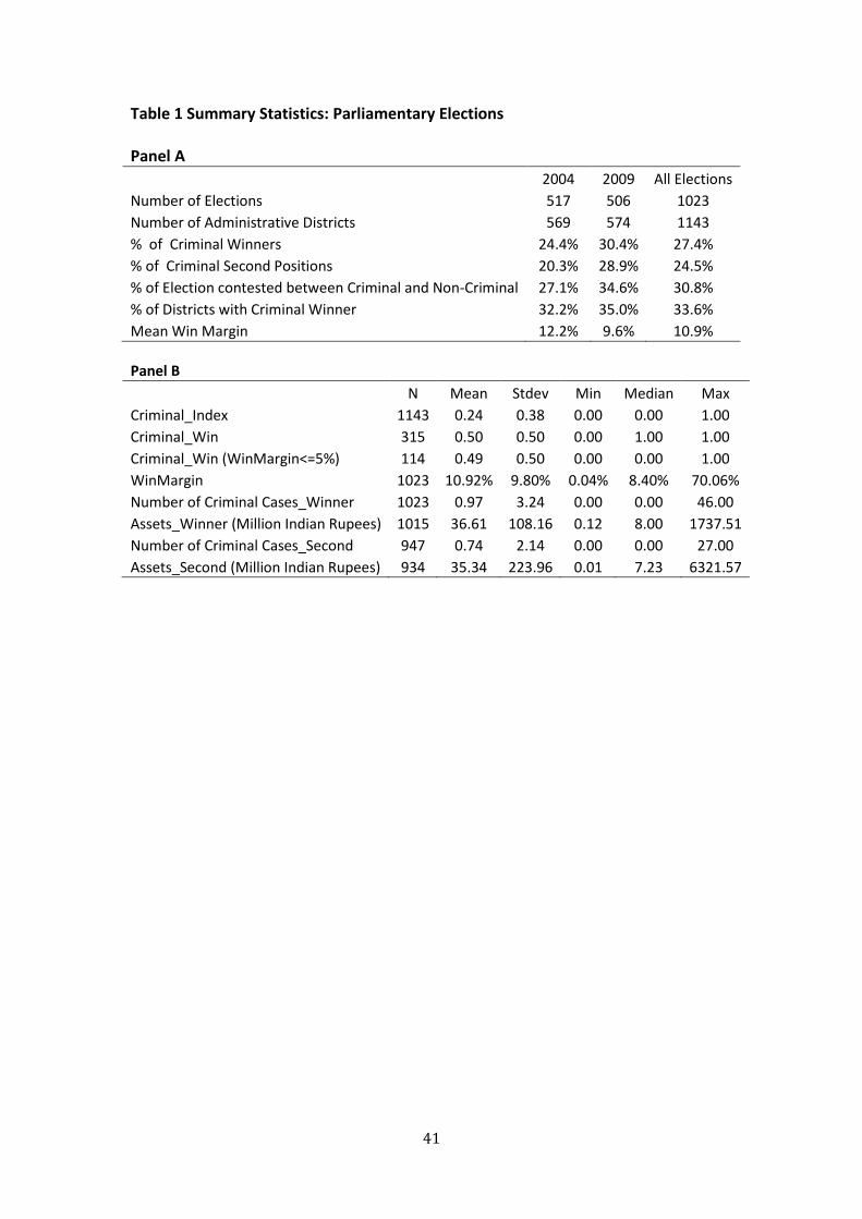
41

Table 1 Summary Statistics: Parliamentary Elections Panel A

2004 2009 All Elections

Number of Elections 517 506 1023

Number of Administrative Districts 569 574 1143

% of Criminal Winners 24.4% 30.4% 27.4%

% of Criminal Second Positions 20.3% 28.9% 24.5%

% of Election contested between Criminal and Non-Criminal 27.1% 34.6% 30.8%

% of Districts with Criminal Winner 32.2% 35.0% 33.6%

Mean Win Margin 12.2% 9.6% 10.9%

Panel B

N Mean Stdev Min Median Max

Criminal_Index 1143 0.24 0.38 0.00 0.00 1.00

Criminal_Win 315 0.50 0.50 0.00 1.00 1.00

Criminal_Win (WinMargin<=5%) 114 0.49 0.50 0.00 0.00 1.00

WinMargin 1023 10.92% 9.80% 0.04% 8.40% 70.06%

Number of Criminal Cases_Winner 1023 0.97 3.24 0.00 0.00 46.00

Assets_Winner (Million Indian Rupees) 1015 36.61 108.16 0.12 8.00 1737.51

Number of Criminal Cases_Second 947 0.74 2.14 0.00 0.00 27.00

Assets_Second (Million Indian Rupees) 934 35.34 223.96 0.01 7.23 6321.57

42

Table 2 Summary Statistics: Firm and Project Variables Panel A

N Mean Stdev Min Median Max

ROA 21424 0.032 0.097 -1.172 0.030 0.629

Q 21436 1.35 1.09 0.18 1.03 17.62

Market Cap 21436 17810.8 119945.4 1.3 543.2 4168660.0

Sales 19607 12111.6 101296.9 0.0 1222.8 4800000.0

Assets 21436 35557.3 291372.3 100.1 1495.7 15689489.6

FII Ownership 21436 3.2% 7.1% 0.0% 0.0% 74.1%

Insider Ownership 21436 45.2% 21.9% 0.0% 48.3% 100.0%

Panel B

N Mean Stdev Min Median Max

Private-Sector Firms

Project Cost (million Indian Rupees) 3400 6409.21 25101.5 100 1120 431490

Project CAR (-1,+1) 3192 1.4% 6.3% -19.0% 0.5% 57.2%

Project CAR(-3,+3) 3192 1.9% 9.2% -30.2% 0.8% 81.6%

Stalled 3400 0.11 0.32 0.00 0.00 1.00

Time to Completion (Days) 1951 747 498 7 640 3375

Total Investment_District 934 81642 189794 0 11690 1646126

Local Invesment_District 934 8667 52802 0 0 755330

Non Local Investment_District 934 72974 164234 0 10462 1304175

State-Owned Firms

Project Cost (million Indian Rupees) 684 23387.5 44280.2 100.0 5204.8 450000.0

Project CAR (-1,+1) 677 0.1% 3.8% -17.3% 0.1% 29.7%

Project CAR(-3,+3) 677 0.4% 5.7% -23.4% 0.0% 26.1%

Stalled 684 0.05 0.22 0.00 0.00 1.00

Time to Completion (Days) 247 1115 594 59 1065 2883

State Ownership 680 73.2% 16.9% 14.0% 80.4% 99.5%

Total Investment_District 805 44128 104402 0 5262 1208036

Local Invesment_District 805 2142 169801 0 0 338500

Non Local Investment_District 805 41986 100762 0 4635 1208036

43

Table 3 Criminal Politicians and Firm Value: Evidence from Project Announcement Returns Panel A

Dependent Variable

Market Model Adjusted CAR(-1,+1) Market Model Adjusted CAR(-3,+3)

Independent Variable LOCAL NON-LOCAL LOCAL NON-LOCAL

1 2 3 4 5 6 7

INTERCEPT 0.019 0.084* -0.119*** 0.033** 0.062 -0.061 0.017

(0.82) (1.84) (3.48) (2.28) (0.77) (1.13) (0.66)

CRIMINAL_INDEX -0.009** -0.009* -0.002 -0.010** -0.017*** -0.017 -0.018*** (2.03) (1.82) (-0.15) (-2.15) (3.03) (0.84) (3.07)

LOG(COST) 0.001 0.001 0.003 0.000 0.000 0.005 -0.001 (0.51) (0.66) (0.58) (0.15) (0.03) (0.71) (0.62)

LOG(MCAP) -0.004*** -0.014*** -0.006** -0.003*** -0.005*** -0.009** -0.005*** (5.23) (2.87) (2.38) (4.80) (4.92) (2.52) (4.29)

R-Square 0.064 0.442 0.152 0.077 0.072 0.195 0.086

Year Fixed Effects Yes Yes Yes Yes Yes Yes Yes

State Fixed Effects Yes No Yes Yes Yes Yes Yes

Industry Fixed Effects Yes No Yes Yes Yes Yes Yes

Firm Fixed Effects No Yes No No No No No

N 3188 3188 636 2552 3188 636 2552

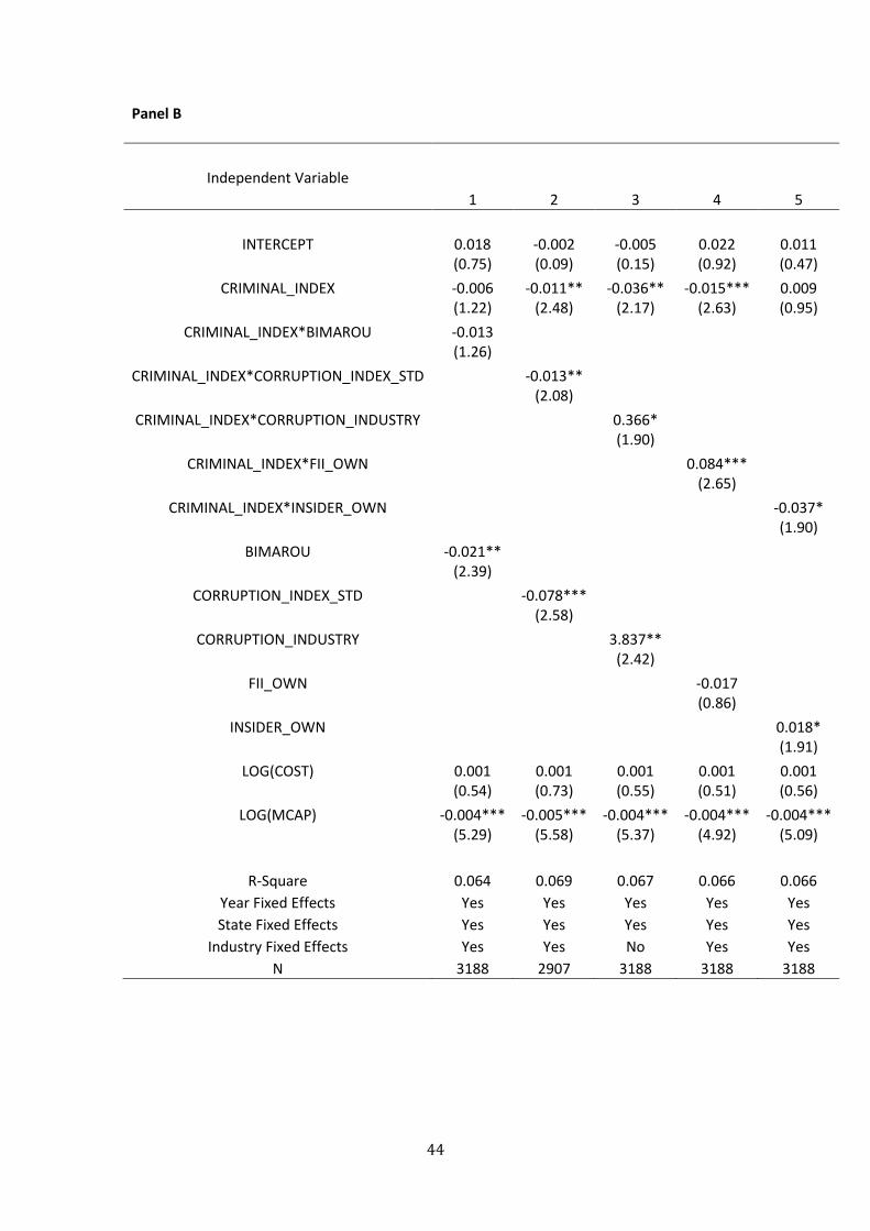
44

Panel B

Independent Variable

1 2 3 4 5

INTERCEPT 0.018 -0.002 -0.005 0.022 0.011 (0.75) (0.09) (0.15) (0.92) (0.47)

CRIMINAL_INDEX -0.006 -0.011** -0.036** -0.015*** 0.009 (1.22) (2.48) (2.17) (2.63) (0.95)

CRIMINAL_INDEX*BIMAROU -0.013 (1.26)

CRIMINAL_INDEX*CORRUPTION_INDEX_STD -0.013** (2.08)

CRIMINAL_INDEX*CORRUPTION_INDUSTRY 0.366* (1.90)

CRIMINAL_INDEX*FII_OWN 0.084*** (2.65)

CRIMINAL_INDEX*INSIDER_OWN -0.037* (1.90)

BIMAROU -0.021** (2.39)

CORRUPTION_INDEX_STD -0.078*** (2.58)

CORRUPTION_INDUSTRY 3.837** (2.42)

FII_OWN -0.017 (0.86)

INSIDER_OWN 0.018* (1.91)

LOG(COST) 0.001 0.001 0.001 0.001 0.001 (0.54) (0.73) (0.55) (0.51) (0.56)

LOG(MCAP) -0.004*** -0.005*** -0.004*** -0.004*** -0.004*** (5.29) (5.58) (5.37) (4.92) (5.09)

R-Square 0.064 0.069 0.067 0.066 0.066

Year Fixed Effects Yes Yes Yes Yes Yes

State Fixed Effects Yes Yes Yes Yes Yes

Industry Fixed Effects Yes Yes No Yes Yes

N 3188 2907 3188 3188 3188

45

Table 4 Criminal Politicians and Project Announcements Returns: Evidence from Close Elections Panel A Private Sector Firms

WINMARGIN<=5%

CAR(-1,+1) % STALL

All NON_LOCAL LOCAL All NON_LOCAL LOCAL

1 2 3 4 5 6

CRIMINAL WIN=0 1.71*** 1.52*** 2.49*** 8.06*** 8.00*** 8.33**

(5.66) (5.07) (2.69) (5.21) (4.65) (2.32)

CRIMINAL WIN=1 0.77*** 0.44 1.60** 10.43*** 11.97*** 6.52**

(2.65) (1.48) (2.33) (6.15) (5.63) (2.52)

DIFF -0.94** -1.08** -0.89 2.37 3.97 -1.81

(-2.24) (2.53) (0.79) (1.03) (1.46) (0.42)

Panel B State-Owned Firms

CAR(-1,+1) % Stall

WINMARGIN<=

5% WINMARGIN<=1

0% WINMARGIN<=

5% WINMARGIN<=1

0%

1 2 3 4

CRIMINAL WIN=0 -0.01 -0.05 10.59*** 9.93***

(0.05) (0.20) (3.15) (4.07) CRIMINAL

WIN=1 0.91*** 0.75*** 2.86 4.92**

(2.81) (3.22) (1.42) (2.50)

DIFF 0.92*** 0.80** -7.73* -5.01

(2.15) (2.29) (1.87) (1.55)

Panel C All Firms

EW CAR(-1,+1) VW CAR(-1,+1) % Stall

WINMARGIN

<=5% <=10% <=5% <=10% <=5% <=10%

1 2 3 4 5 6

CRIMINAL WIN=0 1.34*** 1.31*** 0.30** 0.57*** 8.61*** 9.14***

(5.41) (6.86) (2.09) (4.53) (6.09) (8.45)

CRIMINAL WIN=1 0.80*** 0.79*** 1.32*** 1.12*** 9.09*** 9.17***

(3.26) (3.92) (8.47) (9.44) (6.28) (7.85)

DIFF -0.54 -0.52* 1.02*** 0.55*** 0.48 0.03

(1.56) (1.88) (4.81) (3.12) (0.24) (0.01)

46

Table 5 Criminal Politicians and Project Announcements Returns: Regression Evidence from Close Elections Panel A

Dependent Variable: Market Model-Adjusted CAR (-1,+1)

WINMARGIN<=5% WINMARGIN

<=3% WINMARGIN<

=10% ALL

WINMARGINS Independent

Variable All LOCAL NON-LOCAL NON-LOCAL NON-LOCAL NON-LOCAL

1 2 3 4 5 6

INTERCEPT -0.042 -0.020 0.011 -0.013 0.018 -0.003 (1.58) (0.28) (0.40) (0.42) (1.01) (0.23)

CRIMINALWIN -0.006 0.008 -0.011* -0.010 -0.010*** -0.007** (1.26) (0.57) (1.93) (1.40) (2.72) (2.44)

LOG(COST) 0.000 -0.004 0.002 0.004 -0.001 0.002 (0.03) (0.44) (0.94) (1.31) (0.38) (1.35)

LOG(MCAP) -0.003* -0.009* -0.002 -0.003 -0.001 -0.002** (1.80) (1.94) (1.34) (1.50) (0.87) (2.40)

WIN_MARGIN 0.036 0.392 0.129 0.525 0.051 0.014 (0.21) (0.56) (0.66) (1.09) (0.97) (1.09)

R-Square (%) 13.16 29.6 18.1 28.16 14.4 11.04 Industry Fixed

Effects Yes Yes Yes Yes Yes Yes

State Fixed Effects Yes Yes Yes Yes Yes Yes

Year Fixed Effects Yes Yes Yes Yes Yes Yes Clustered(District,

ElectionYear) Yes Yes Yes Yes Yes Yes

N 614 148 466 316 770 1474

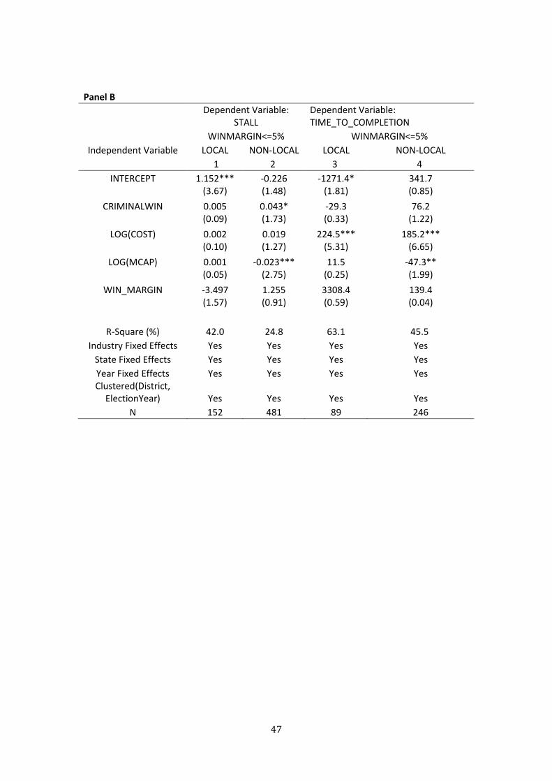
47

Panel B

Dependent Variable:

STALL Dependent Variable: TIME_TO_COMPLETION

WINMARGIN<=5% WINMARGIN<=5%

Independent Variable LOCAL NON-LOCAL LOCAL NON-LOCAL

1 2 3 4

INTERCEPT 1.152*** -0.226 -1271.4* 341.7 (3.67) (1.48) (1.81) (0.85)

CRIMINALWIN 0.005 0.043* -29.3 76.2 (0.09) (1.73) (0.33) (1.22)

LOG(COST) 0.002 0.019 224.5*** 185.2*** (0.10) (1.27) (5.31) (6.65)

LOG(MCAP) 0.001 -0.023*** 11.5 -47.3** (0.05) (2.75) (0.25) (1.99)

WIN_MARGIN -3.497 1.255 3308.4 139.4 (1.57) (0.91) (0.59) (0.04)

R-Square (%) 42.0 24.8 63.1 45.5

Industry Fixed Effects Yes Yes Yes Yes

State Fixed Effects Yes Yes Yes Yes

Year Fixed Effects Yes Yes Yes Yes Clustered(District,

ElectionYear) Yes Yes Yes Yes

N 152 481 89 246

48

Panel C State-Owned Firms

Dependent Variable: Market Model-Adjusted CAR (-1,+1)

WINMARGIN<=5% WINMARGIN<=10%

Independent Variable All

GOVT OWN>=70

% GOVT

OWN<70% All

GOVT OWN>=70

%

GOVT OWN<70

%

1 2 3 4 5 6

INTERCEPT -0.026 -0.154** 0.081 -0.053 0.098* -0.038 (0.44) (2.17) (1.11) (1.14) (1.72) (0.72)

CRIMINALWIN 0.001 0.011*** -0.008 0.007** 0.010*** -0.003 (0.31) (2.63) (1.13) (2.51) (2.69) (0.84)

LOG(COST) 0.006*** 0.004* 0.008*** 0.004*** 0.004*** 0.008*** (4.69) (1.76) (3.98) (3.44) (2.65) (4.60)

LOG(MCAP) -0.002 0.008 -0.011** 0.000 0.001 -0.004 (0.57) (1.34) (2.07) (0.08) (0.09) (1.00)

WIN_MARGIN 0.269 0.753*** -0.479 -0.023 0.007 0.020 (1.34) (3.03) (1.31) (0.51) (0.11) (0.44)

R-Square (%) 46.34 75.0 68.7 34.84 52.4 67.23

Industry Fixed Effects Yes Yes Yes Yes Yes Yes

State Fixed Effects Yes Yes Yes Yes Yes Yes

Year Fixed Effects Yes Yes Yes Yes Yes Yes Clustered(District,

ElectionYear) Yes Yes Yes Yes Yes Yes

N 154 86 68 272 160 112

49

Table 6 Project Announcement Returns: Corrupt States and Firms’ Ownership Structure

Dependent Variable: Market Model-Adjusted CAR (-1,+1)

WINMARGIN<=5%

Independent Variable NON-LOCAL NON-LOCAL NON-LOCAL NON-LOCAL NON-LOCAL NON-LOCAL

1 2 3 4 5 6

INTERCEPT 0.006 0.003 0.065* 0.052 0.027 0.020

(0.21) (0.12) (1.85) (1.80) (0.99) (0.70)

CRIMINALWIN -0.008 -0.013** -0.030* -0.063** -0.017** 0.006 (1.25) (-2.49) (1.75) (2.48) (2.31) (0.56)

CRIMINALWIN*BIMAROU -0.012 (0.97)

CRIMINALWIN*CORRUPTION_INDEX_STATE -0.016** (-2.47)

CRIMINALWIN*CORRUPTION_INDUSTRY 0.252 (1.34)

CRIMINALWIN*LOGMCAP 0.006** (1.98)

CRIMINALWIN*FII_OWN

0.000 0.001

(0.01) (1.18)

CRIMINALWIN*INSIDER_OWN

-0.039** (1.98)

BIMAROU -0.001 (0.07)

CORRUPTION_INDEX_STATE

-0.014

(0.26)

CORRUPTION_INDEX_INDUSTRY

-0.633** (2.03)

FII_OWN

0.001* 0.000 (1.79) (1.00)

50

INSIDER_OWN 0.005

(0.38)

LOG(COST) 0.002 0.002 0.002 0.002 0.002 0.002 (0.96) (0.96) (0.87) (0.91) (0.94) (1.02)

LOG(MCAP) -0.002 -0.003 -0.003 -0.007*** -0.004** -0.003 (1.33) (1.44) (1.51) (3.37) (2.20) (1.49)

WIN_MARGIN 0.163 0.187

0.072 0.115 0.099 (0.78) (0.96) (0.35) (0.58) (0.49)

R-Square (%) 18.31 19.2 18.7 20.4 19.6 19.31

Industry Fixed Effects Yes Yes Yes Yes Yes Yes

State Fixed Effects Yes Yes Yes Yes Yes Yes

Year Fixed Effects Yes Yes Yes Yes Yes Yes

Clustered(District, ElectionYear) Yes Yes Yes Yes Yes Yes

N 466 466 466 466 466 466

51

Table 7 Political Party Affiliation and Project Announcement Returns

Dependent Variable: Market Model-Adjusted CAR (-1,+1)

WINMARGIN<=5%

NATIONAL_PARTIES OTHERS

Independent Variable NON-LOCAL NON-LOCAL NON-LOCAL NON-LOCAL

1 2 3 4

INTERCEPT 0.016 0.009 0.0146 -0.006

(0.63) (0.34) (0.49) (0.12)

CRIMINALWIN -0.019*** -0.022 -0.0121* -0.013 (3.00) (3.05) (1.80) (1.41)

CRIMINALWIN*STATE_GOVT 0.018**

(2.18)

CRIMINALWIN*CENTRAL_GOVT

0.024**

(2.57)

STATE_GOVT -0.017***

(2.72)

CENTRAL_GOVT

-0.007

(1.08)

LOG(COST) 0.002 0.002 -0.0005 0.005 (1.01) (1.08) (0.15) (1.66)

LOG(MCAP) -0.002 -0.002 0.0004 -0.004 (1.02) (1.21) (0.21) (1.27)

WIN_MARGIN 0.088 0.166 -0.5312* 0.555 (0.45) (0.84) (-1.93) (1.38)

R-Square (%) 19.61 19.7 30.7 21.0

Industry Fixed Effects Yes Yes Yes Yes

State Fixed Effects Yes Yes Yes Yes

Year Fixed Effects Yes Yes Yes Yes

Clustered(District, ElectionYear) Yes Yes Yes Yes

N 502 502 256 210

52

Table 8 Criminal Politicians and Aggregate Investments around Close Elections Panel A

WINMARGIN<=0.05 WINMARGIN<=0.10

Independent Variable ChangeTotal Project Cost

Change Local

Project Cost

Change Non-Local

Project Cost

ChangeTotal Project Cost

Change Local

Project Cost

Change Non-Local

Project Cost

1 2 3 4 5 6

CRIMINAL_WIN=0 28049.6 8857.1 19192.5 13044.3 7087.0* 5957.3

(1.33) (1.41) (0.97) (0.77) (1.81) (0.37)

CRIMINAL_WIN=1 -38394.5 -938.1 -37456.4* -39121.3** 1502.5 -40623.8** (1.63) (0.34) (1.67) (2.12) (0.34) (2.37)

DIFF -66444.1** -9795.2 -56648.9* -52165.6** -5584.5 -46581.1** (2.11) (1.39) (1.90) (2.08) (0.95) (1.97)

Panel B

Dependent Variable

WINMARGIN<=5% WINMARGIN<=10%

Independent Variable ChangeTotal Project Cost

Change Local Project Cost

Change Non-Local Project

Cost ChangeTotal Project Cost

1 2 3 4

INTERCEPT -190869.5 9806.0 -200675.5 -175313.0

(1.38) (1.29) (1.49) (1.27)

CRIMINAL_WIN -93006.5** -20195.3 -72811.1* -68243.1**

(2.16) (1.61) (1.81) (2.26)

R-Square (%) 11.81 13.0 10.6 9.59

State Fixed Effects Yes Yes Yes Yes

Clustered(District, ElectionYear) Yes Yes Yes Yes

N 164 164 164 275

53

Panel C

State Owned Firms All Firms

WINMARGIN<=5% WINMARGIN<=10% WINMARGIN<=5% WINMARGIN<=10%

Independent Variable ChangeTotal Project Cost

ChangeTotal Project Cost

ChangeTotal Project Cost

ChangeTotal Project Cost

1 2 3 4

CRIMINAL_WIN=0 -23216.3 -271.0 6664.2 11681.1

(-0.99) (-0.02) (0.23) (0.55)

CRIMINAL_WIN=1 21905.6** 23538.5** -16793.9 -15921.1

(2.03) (2.40) (-0.75) (-0.89)

DIFF 45121.9* 23809.5 -23458.1 -27602.2

(1.70) (1.28) (-0.64) (-0.98)

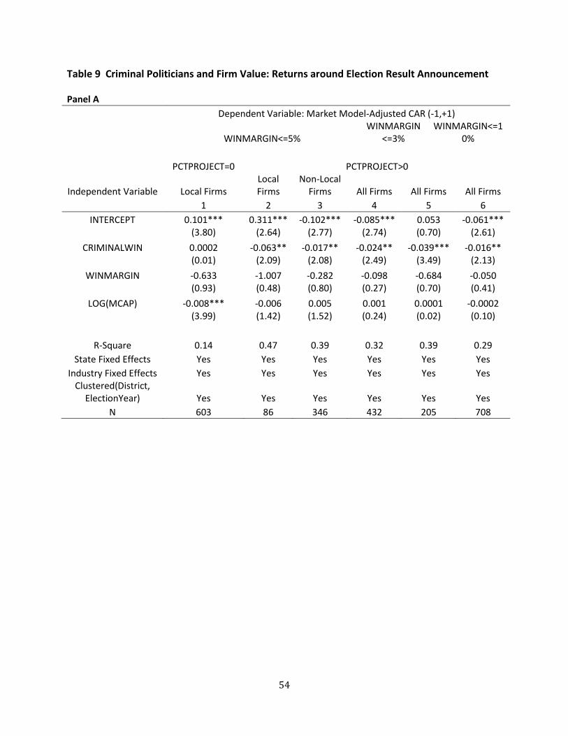
54

Table 9 Criminal Politicians and Firm Value: Returns around Election Result Announcement Panel A

Dependent Variable: Market Model-Adjusted CAR (-1,+1)

WINMARGIN<=5% WINMARGIN

<=3% WINMARGIN<=1

0%

PCTPROJECT=0 PCTPROJECT>0

Independent Variable Local Firms Local Firms

Non-Local Firms All Firms All Firms All Firms

1 2 3 4 5 6

INTERCEPT 0.101*** 0.311*** -0.102*** -0.085*** 0.053 -0.061***

(3.80) (2.64) (2.77) (2.74) (0.70) (2.61)

CRIMINALWIN 0.0002 -0.063** -0.017** -0.024** -0.039*** -0.016** (0.01) (2.09) (2.08) (2.49) (3.49) (2.13)

WINMARGIN -0.633 -1.007 -0.282 -0.098 -0.684 -0.050 (0.93) (0.48) (0.80) (0.27) (0.70) (0.41)

LOG(MCAP) -0.008*** -0.006 0.005 0.001 0.0001 -0.0002 (3.99) (1.42) (1.52) (0.24) (0.02) (0.10)

R-Square 0.14 0.47 0.39 0.32 0.39 0.29

State Fixed Effects Yes Yes Yes Yes Yes Yes

Industry Fixed Effects Yes Yes Yes Yes Yes Yes Clustered(District,

ElectionYear) Yes Yes Yes Yes Yes Yes

N 603 86 346 432 205 708

55

Panel B

Dependent Variable: Market Model-Adjusted CAR (-1,+1)

WINMARGIN<=5%

Independent Variable All Firms with PCTPROJECT>0

1 2 3 4 5 6

INTERCEPT -0.104*** -0.085*** -0.086*** -0.066** -0.079 -0.046

(2.90) (2.87) (3.06) (2.15) (2.47) (1.28)

CRIMINALWIN -0.012 -0.040*** -0.022* -0.024*** -0.013 -0.059 (1.22) (3.54) (1.90) (2.72) (1.21) (3.23)

WINMARGIN -0.067 -0.005 -0.026 -0.110 -0.226 -0.122 (0.19) (0.02) (0.07) (0.30) (0.60) (0.35)

LOG(MCAP) 0.001 0.000 0.000 0.001 -0.003 0.000 (0.57) (0.04) (0.05) (0.34) (1.08) (0.19)

CRIMINALWIN*CRIMINAL_INCUMBENT -0.040** (2.11)

CRIMINALWIN*MINISTER 0.033 (1.57)

CRIMINALWIN*STATEGOVT 0.010 (0.89)

CRIMINALWIN*CORRUPTION_INDEX_STATE -0.011 (1.07)

CRIMINALWIN*FII_OWN -0.123 (1.34)

CRIMINALWIN*INSIDER_OWN 0.080** (2.07)

CRIMINAL_INCUMBENT 0.030** (2.33)

MINISTER -0.014 (0.61)

STATE_GOVT -0.011 (0.97)

56

CORRUPTION_INDEX_STATE

0.078 (0.92)

FII_OWN 0.209*** (2.59)

INSIDER_OWN -0.075*** (2.87)

R-Square 0.32 0.33 0.38 0.32 0.33 0.33

State Fixed Effects Yes Yes Yes Yes Yes Yes

Industry Fixed Effects Yes Yes Yes Yes Yes Yes

Clustered(District, ElectionYear) Yes Yes Yes Yes Yes Yes

N 432 463 557 432 432 432

57

Table 10 Election of Criminal Politicians: Effects on Firm Value and Profitability

Independent Variable Q Q Q ROA ROA ROA

1 2 3 4 5 6

CRIMINAL_INDEX -0.067***

-0.043 -0.001

0.0000 (2.63) (1.60) (0.45) (0.01)

LOG(1+CRIMINAL_CASES)

-0.040**

-0.004* (2.01) (1.69)

CRIMINAL_INDEX*PCTPROJECTS

-0.222***

-0.0085 (2.74) (0.90)

PCTPROJECTS

0.031

-0.0103** (0.70) (2.02)

LOG(SALES) 0.008 0.008 0.008 0.010*** 0.010*** 0.0101*** (1.21) (1.28) (1.27) (13.18) (13.25) (13.33)

R-Square 0.68 0.68 0.68 0.51 0.51 0.51

Firm Fixed Effects Yes Yes Yes Yes Yes Yes

N 19510 19510 19510 19510 19510 19510

58

Table 11 Tobin’s Q and ROA regressions: Evidence from close elections

Win Margin <=0.03 Win Margin <=0.05 Win Margin <=0.10

All Elections All Elections All Elections

Independent Variable Q ROA Q ROA Q ROA

1 2 3 4 5 6

INTERCEPT -0.472* -0.095*** -0.496*** -0.086*** -0.520*** -0.083*** (1.95) (3.29) (4.58) (5.78) (4.47) (6.76)

CRIMINAL_WIN -0.046 0.007 0.054 0.010** 0.058* 0.006* (0.49) (0.65) (0.94) (2.14) (1.68) (1.65)

CRIMINAL_WIN*POST -0.135** -0.017* -0.098 -0.006 -0.067 -0.006 (1.97) (1.85) (1.60) (1.20) (1.23) (1.64)

POST 0.251** 0.022** 0.138** 0.016*** 0.086 0.007 (2.14) (2.01) (2.16) (3.04) (1.00) (1.56)

LOG(SALES) 0.049** 0.010*** 0.054*** 0.009*** 0.057*** 0.009*** (2.28) (3.62) (4.59) (9.47) (3.72) (9.50)

R-Square 0.09 0.063 0.058 0.05 0.05 0.06

State Fixed Effects Yes Yes Yes Yes Yes Yes

Year Fixed Effects Yes Yes Yes Yes Yes Yes

N 2317 2317 7717 7717 11899 11899

59

Appendix 1 Regression Discontinuity Design: Tests Panel A Criminal Candidate Characteristics around the Cutoff Point

Intercept Criminal Win

Number of Criminal Cases 2.66*** -0.03 (4.81) (0.04)

Serious Criminal 0.50*** -0.05 (7.55) (0.57)

Assets 66.65*** -37.95 (2.89) (1.58)

Liabilities 4.161* -0.986 (1.74) (0.38)

Education 3.931*** -0.181 (27.06) (0.89)

National Party 0.569*** 0.11 (8.67) (1.21)

Panel B Outcome variables around alternative cutoff points

Project Ann Election Ann Change Investment

CAR(-1,+1) CAR(-1,+1) Change Total Project

Cost

+5% -5% +5% -5% +5% -5%

Intercept -0.004 0.049** -0.131*** -0.044 741.8 -362407.6*

(0.11) (2.08) (5.60) (1.41) (0.01) (1.87)

CRIMINAL_WIN 0.014 -0.012 -0.018 0.001 14141.0 -27929.5

(1.51) (1.08) (0.92) (0.02) (0.44) (0.69)

WINMARGIN -0.248 0.264 0.248 -0.133

(1.11) (1.29) (0.74) (0.27)

LOG(MCAP) 0.001 -0.003* 0.001 -0.001

(0.42) (1.78) (0.39) (0.32)

Clustered(District,Election

Year) Yes Yes Yes Yes Yes Yes

Industry Fixed Effects Yes Yes Yes Yes No No

State Fixed Effects Yes Yes Yes Yes Yes Yes

Year Fixed Effects Yes Yes No No No No

N 347 423 356 352 129 146

R2 21.26 22.27 43.36 22.7 24.51 23.76

60

Figure 1 Criminal Politicians Index: 2009 General Election (Note: White shaded area indicates that the district has zero elected MPs with criminal background. Light Gray indicates less than or equal to half of the elected MPs with a criminal background whereas dark gray indicates districts with more than half of the MPs with criminal charges.

61

Figure 2 Panel A Regression Discontinuity Design: Distribution of Vote-Share Difference

Figure 2 Panel B Smoothed Density of Vote-Share Difference

0

.02

.04

.06

Den

sity

-50 0 50Vote Difference (%)

0

.01

.02

.03

.04

.05

Den

sity

-100 -50 0 50 100Vote Difference (%)

62

Figure 3 Panel A Project Announcement Returns: Private Sector Firms

Figure 3 Panel B Project Announcement Returns: Private Sector Firms (Including Year Fixed-Effects)

-10

12

3

Ma

rket-

ad

juste

d A

bn

orm

al (-

1,+

1)

Retu

rn (

%)

-10 -5 0 5 10Win Margin (%)

0.5

11

.52

2.5

Ma

rket-

ad

juste

d A

bn

orm

al (-

1,+

1)

Retu

rn (

%)

-10 -5 0 5 10Win Margin (%)

63

Figure 3 Panel C Project Announcement Returns: State-Owned Firms (Including Year Fixed-Effects)

-1-.

50

.51

Ma

rket-

ad

juste

d A

bn

orm

al (-

1,+

1)

Retu

rn (

%)

-10 -5 0 5 10Win Margin (%)

64

Figure 4 Panel A Change Total Project Cost: Private Sector

Figure 4 Panel B Change Total Project Cost: Private Sector (Including State-Fixed Effects)

-100

00

0-5

00

00

0

500

00

Cha

ng

e T

ota

l P

roje

ct C

ost (M

illio

n In

dia

n R

up

ee

s)

-10 -5 0 5 10Win Margin (%)

-600

00

-400

00

-200

00

0

200

00

400

00

Cha

ng

e T

ota

l P

roje

ct C

ost (M

illio

n In

dia

n R

up

ee

s)

-10 -5 0 5 10Win Margin (%)

65

Figure 5 Election Result Announcement Returns around Close Elections

-2-1

01

2

Ma

rket-

ad

juste

d A

bn

orm

al (-

1,+

1)

Retu

rn (

%)

-10 -5 0 5 10Win Margin (%)