criminal careers of public places - center for · pdf file · 2008-01-23frequent...
TRANSCRIPT
CRIMINAL CAREERS OF PUBLIC
PLACES
by
William SpelmanUniversity of Texas at Austin
Abstract: Most police calls for service come from especially dangerouslocations, or "hot spots." If risks at these locations are stable—hot spots stayhot—community problem-solving techniques may reduce crimes and disor-ders substantially. If locations run high risks only temporarily or sporadi-cally, location-based strategies may not work. Analysis of calls for serviceat high schools, housing projects, subway stations and parks in Bostonshows that risks remain fairly constant over time; most apparent changesmay be attributed to random processes. Autoregression and displacement inspace and call type are statistically significant but unimportant indicators ofcall rates. In addition to verifying the effectiveness of community problem-solving strategies, these results have practical implications for problem-solv-ing techniques.
CRIMINAL CAREERS OF PUBLIC PLACES
Over the past decade, research has confirmed what many criminaljustice practitioners always knew: a few, particularly frequent, offendersare responsible for a disproportionate amount of crime (Chaiken andChaiken, 1982; Horney and Marshall, 1991: Mande and English, 1988).Such findings have led to calls for "selective incapacitation," aimed atimprisoning the frequent few and—presumably—preventing the crimes inwhich they would have participated, had they been free (Blumstein et al.,1986: Zedlewski, 1987).
Nevertheless, three elements are required before a crime can becommitted. Not only must someone be motivated to commit it, but asuitable target must be available, in a (relatively) unguarded location,providing the offender with an opportunity to commit the crime (Cohenand Felson, 1979). Recent research suggests that, like offenders, somevictims and places are particularly crime-prone. Some individuals run
Address correspondence to: William Spelman, Lyndon B. Johnson School of PublicAffairs. University of Texas. P.O. Box Y. Austin, TX 78713-7450.
115
116 William Spelman
especially high risks of becoming victims—people in dangerous jobs, forexample, or women in abusive personal relationships (Nelson, 1984; Reiss,1980). And some locations run especially high risks of being the site ofvictimizations (Pierce et al.. 1986; Sherman et al., 1989).
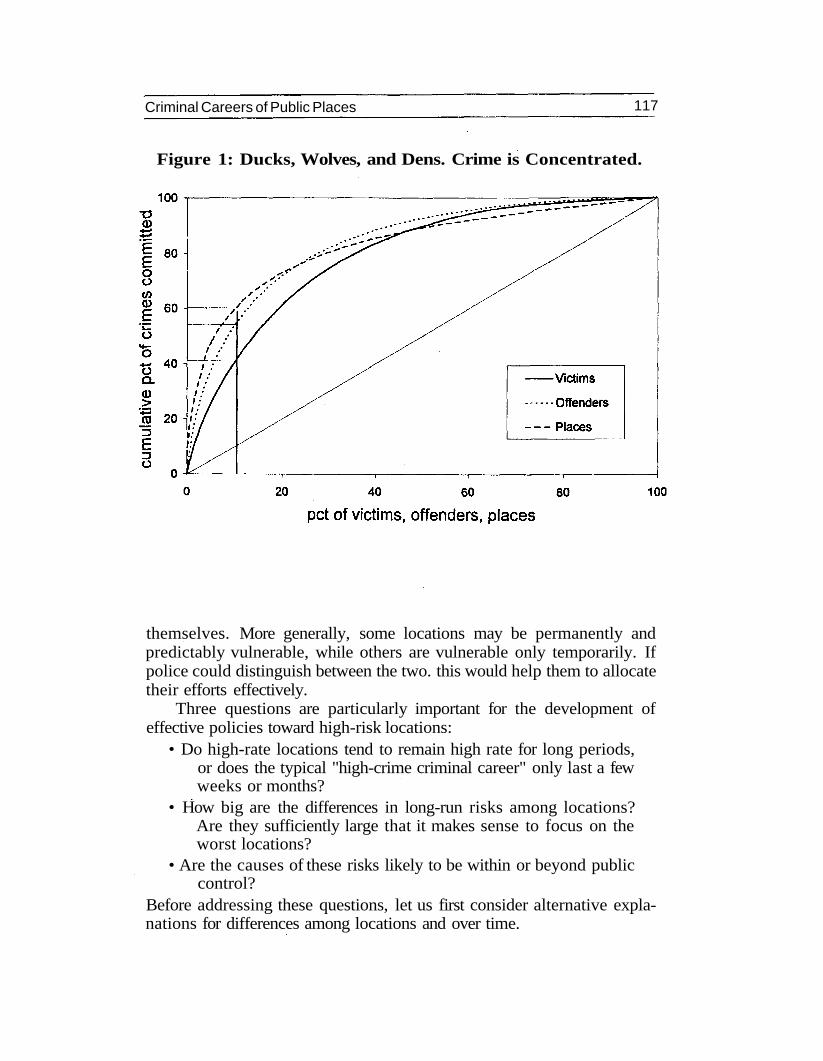
To measure the importance of these high-risk cases, suppose we tookall the criminals active in a community and lined them up in order of thefrequency with which they committed crimes. Those who committedcrimes most often would go to the head of the line; those who committedcrimes only occasionally would go to the end. If all offenders were alike,then it would not matter much where we would line each one of them up;the offenders at the front of the line would commit about as many crimesas those at the end. For example, the "worst" 10% of criminals wouldaccount for about 10% of all crimes. But if there were significant differ-ences among offenders, those at the head of the line would account for farmore than their share of all crimes committed; the worst 10% wouldaccount for much more than 10% of all crimes.
Figure 1 shows what happens if we conduct such an experiment withavailable data on repeat offending, repeat victimization and repeat callsfor service. Surveys of jail and prison inmates suggest that the mostfrequent 10% of offenders are responsible for about 55% of all street crimescommitted (Blumstein et al., 1986; Chaiken and Chaiken, 1982; Clarkeand Weisburd, 1992). According to the National Crime Survey, the 10% ofpotential victims at highest risk account for over 40% of all victimizations(Nelson, 1984; see also Fienberg, 1980; Reiss, 1980). Calls-for-service datain Boston and Minneapolis show that the addresses producing the mostrepeat calls account for over 60% of all calls (Pierce et al., 1986; Shermanet al., 1989).
These "sitting ducks" and "dens of iniquity" not only form a symmetrywith the "ravenous wolves" of frequent offending; they also have policyimplications of their own. Many innovative police departments haveadopted community- and problem-oriented approaches, in large part todeal with persistent victimization problems (Goldstein, 1990; Greene andMastrofski, 1988). With the support of the U.S. National Institute ofJustice, the Minneapolis Police Department even formed a special squadaimed at solving problems at high-risk locations (Sherman et al., 1989).
Like selective incapacitation, however, such "repeat-call" strategieswork only if the crime- and disturbance-prone addresses would haveremained crime- and disturbance-prone in the absence of police action. Ifthe typical high-risk location only remains vulnerable for a few weeks ormonths, for example, then time-consuming police efforts to solve theproblems that caused the vulnerability may be unnecessary: by the timethe police have identified a solution, the problems would have solved
Criminal Careers of Public Places 117
Figure 1: Ducks, Wolves, and Dens. Crime is Concentrated.
themselves. More generally, some locations may be permanently andpredictably vulnerable, while others are vulnerable only temporarily. Ifpolice could distinguish between the two. this would help them to allocatetheir efforts effectively.
Three questions are particularly important for the development ofeffective policies toward high-risk locations:
• Do high-rate locations tend to remain high rate for long periods,or does the typical "high-crime criminal career" only last a fewweeks or months?
• How big are the differences in long-run risks among locations?Are they sufficiently large that it makes sense to focus on theworst locations?
• Are the causes of these risks likely to be within or beyond publiccontrol?
Before addressing these questions, let us first consider alternative expla-nations for differences among locations and over time.
118 William Spelman
WHAT MAKES HOT SPOTS HOT?
Consider a typical police spot map. Each day, the previous day's crimesare marked on the map. Over the course of a month, some locations willhave racked up many more spots than others—that month's "hot spots."Since the police department has limited resources, it might reasonablydecide to assign only the hottest locations to community problem solvers.But depending on what makes each hot spot hot, such a strategy may becompletely ineffective. To see why, consider four reasons why hot spotsmay get hot.
Random Error. Assembly lines are reliable; General Motors' Saturnplant cranks out a completed automobile every eight minutes. Not so thesocial processes that produce crimes, disturbances and other calls forservice. As any patrol officer knows, there is a chance of a call coming infrom anywhere, at any time. Even if some places and times are more likelyto produce calls than others, the unpredictability remains.
Figure 2A shows how chance can make a location look hot. Over thelong run, the same number of crimes were reported each month during1977 and 1978 at Commonwealth as at Bunker Hill, two large Bostonhousing projects. Further, the average number of incidents reported eachmonth did not change over time. Yet because incidents are random, theactual number reported each month did change over time; during somemonths, Commonwealth looked like the hot spot, while other monthsBunker Hill looked hotter. But this is an illusion, caused by the randomnature of crime.
Citywide seasons and trends can also make a location look hot for shortperiods. Particularly in a northern city such as Boston, we might expectmore calls anywhere during the summer than the winter, and more callsduring an especially dry and mild spring. In many cities the overall trendis toward more calls over time. So another reason a location may lookespecially hot at some time is that all locations are hot. In this case, it maybe necessary to devote more than the usual resources to handle all of theincidents, but any attempt to solve the underlying problems would bedoomed to imaginary success. The "problem" is nice weather or some othercitywide condition that will not respond to local changes in the physicalor social environment.
Figure 2B shows the number of disturbance calls reported for theCommonwealth and M.E. McCormack housing projects in Boston. Bothhave the expected pattern, peaking in the summer and bottoming out in

120 William Spelman
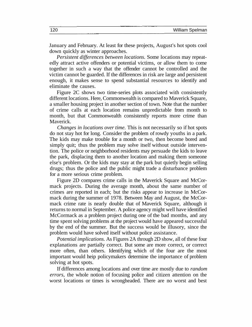
January and February. At least for these projects, August's hot spots cooldown quickly as winter approaches.
Persistent differences between locations. Some locations may repeat-edly attract active offenders or potential victims, or allow them to cometogether in such a way that the offender cannot be controlled and thevictim cannot be guarded. If the differences in risk are large and persistentenough, it makes sense to spend substantial resources to identify andeliminate the causes.
Figure 2C shows two time-series plots associated with consistentlydifferent locations. Here, Commonwealth is compared to Maverick Square,a smaller housing project in another section of town. Note that the numberof crime calls at each location remains unpredictable from month tomonth, but that Commonwealth consistently reports more crime thanMaverick.
Changes in locations over time. This is not necessarily so if hot spotsdo not stay hot for long. Consider the problem of rowdy youths in a park.The kids may make trouble for a month or two, then become bored andsimply quit; thus the problem may solve itself without outside interven-tion. The police or neighborhood residents may persuade the kids to leavethe park, displacing them to another location and making them someoneelse's problem. Or the kids may stay at the park but quietly begin sellingdrugs; thus the police and the public might trade a disturbance problemfor a more serious crime problem.
Figure 2D compares crime calls in the Maverick Square and McCor-mack projects. During the average month, about the same number ofcrimes are reported in each; but the risks appear to increase in McCor-mack during the summer of 1978. Between May and August, the McCor-mack crime rate is nearly double that of Maverick Square, although itreturns to normal in September. A police agency might well have identifiedMcCormack as a problem project during one of the bad months, and anytime spent solving problems at the project would have appeared successfulby the end of the summer. But the success would be illusory, since theproblem would have solved itself without police assistance.
Potential implications. As Figures 2A through 2D show, all of these fourexplanations are partially correct. But some are more correct, or correctmore often, than others. Identifying which of the four are the mostimportant would heip policymakers determine the importance of problemsolving at hot spots.
If differences among locations and over time are mostly due to randomerrors, the whole notion of focusing police and citizen attention on theworst locations or times is wrongheaded. There are no worst and best

Criminal Careers of Public Places 121
places and times, no "problems" to be "solved" and nothing to be gainedby focusing our resources.
If many of the differences can be accounted for by seasons and trends,citywide efforts are called for. We need more police officers, better commu-nity guardianship and more cautious potential victims at some times thanothers. It may help to focus our efforts on some locations, since this maybe a more efficient means of getting the message across to the public. Butall locations are alike, and changing the characteristics of these locationsis itself unlikely to prove useful.
The opposite is true if most of the variation is due to persistentdifferences among locations. In this case, there is something about theindividual place that produces more or fewer crimes, disturbances andpersons in need of service. The key to call reduction lies in the identifica-tion and solution of very localized problems. Further, because risks aremore or less fixed we can have some faith that once solved, problems willstay solved.
Finally, we must take a mixed approach if differences among locationsare large but changing over time. Problems come and go; even if we do nottake great pains to solve them, they will (eventually) solve themselves. Thisis especially true if spatial displacement appears to be an important causeof changes in risks. It is less true if high-risks locations are liable to remainhigher than average for several months before returning to normal. Ingeneral, the implications depend greatly on the nature of the temporalchanges, and more analysis is likely to be needed if this explanation iscorrect.
Given these general policy guidelines, let us now turn our attention tothe empirical evidence.
DATA
Boston represents a particularly good test of these four alternatives.Until the early 1980s, the Boston Police Department (BPD) took an almostentirely incident-driven approach to policing. Swamped by 911 calls, BPDofficers—like those in most jurisdictions—had little time to identify,analyze and solve problems on their beats. Although the focus has shiftedover the last decade, the pattern during the late 1970s is probably muchlike that facing incident-driven police agencies nationwide.
The data set consists of calls for police service reported betweenJanuary 1977 and December 1980 and recorded by the BPD's computer-
122 William Spelman
aided dispatch system (Pierce et al., 1986). All calls for service wereexamined for:
• 35 public and private high schools,
• 35 public housing projects,
• 53 subway stations, and
• 135 parks and playgrounds.
Public places were chosen for several reasons. They are easy to identify.Each type is relatively homogeneous; for example, all high schools aresimilar enough that we can expect their hot-spot characteristics to be aboutthe same. Because it is hard to restrict access to any of them, theenvironment should be especially important to problem solvers. Finally,over the four-year period each of these four types of public places producedfar more than their share of calls for service.
Calls for service were chosen for study because they include a widervariety of problems than reported crime data, and many of the problemsinvolving crime have serious costs for the police and the public. Forexample, nonviolent domestic disputes sometimes escalate into dangeroussituations. In addition, juvenile disturbances may cause little tangibleharm, but they increase fear of crime by creating an impression that thingsare out of control.
The nature of each call was recoded to fit one of three categories: crime,disturbance and service. This means that each category includes a widevariety of incidents; for example, assault, auto theft and drug dealing areall classified as crimes. If each of these crimes behaves differently—hotspots for auto theft are permanent while hot spots for drug dealing movearound, for instance—our results may be misleading. Nevertheless, largecategories were a practical necessity to keep the analysis from becomingtoo complicated. Table 1 shows the nature of the calls produced by eachlocation type.
Finally, the time and date the call was received was recoded. Sincemany of the locations of each type generated relatively few calls, relativelylong time periods were chosen for study—28 days. Each period thusincludes the same number of weekdays and weekends, making themeasier to compare.
Before continuing, it is important to recognize the limitations of thisdata set. Boston is a fairly dense, northern city with a good public transitnetwork. Therefore, we can expect more evidence of seasonality and spatialdisplacement here than in other places. Simply because they are open tothe public, we might expect the criminal careers of public places to bedifferent from the careers of, say, single-family houses or office buildings.

Criminal Careers of Public Places 123
Table 1: Nature of Calls Received by Location Type
124 William Spelman
We might also expect them to be different from retail stores or bars; eventhough open to the public, the private owners of these locations mayrespond more quickly and effectively than the police and the public tochanges in risks. So we may extend these results to other places andproblems only at some risk.

Criminal Careers of Public Places 125
126 William Spelman
Criminal Careers of Public Places 127
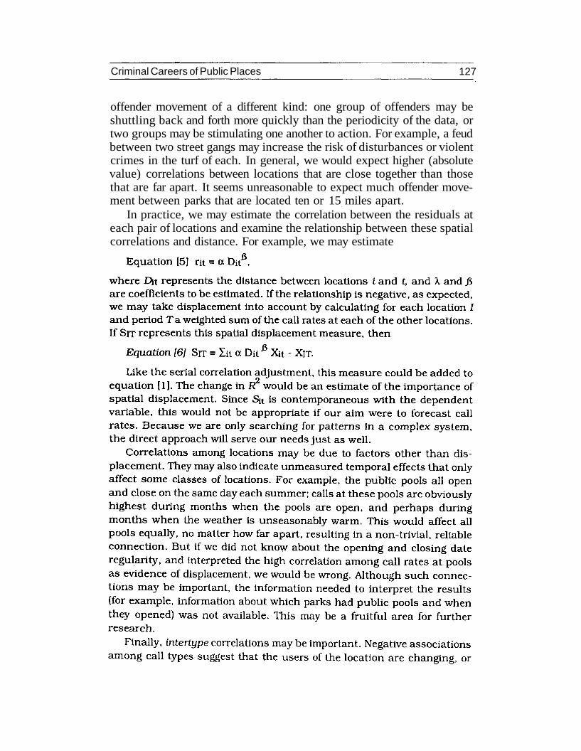
offender movement of a different kind: one group of offenders may beshuttling back and forth more quickly than the periodicity of the data, ortwo groups may be stimulating one another to action. For example, a feudbetween two street gangs may increase the risk of disturbances or violentcrimes in the turf of each. In general, we would expect higher (absolutevalue) correlations between locations that are close together than thosethat are far apart. It seems unreasonable to expect much offender move-ment between parks that are located ten or 15 miles apart.
In practice, we may estimate the correlation between the residuals ateach pair of locations and examine the relationship between these spatialcorrelations and distance. For example, we may estimate
128 William Spelman
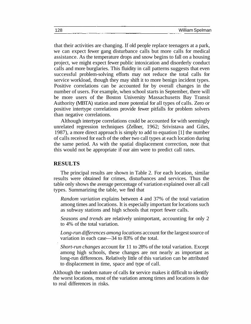
that their activities are changing. If old people replace teenagers at a park,we can expect fewer gang disturbance calls but more calls for medicalassistance. As the temperature drops and snow begins to fall on a housingproject, we might expect fewer public intoxication and disorderly conductcalls and more burglaries. This fluidity in call patterns suggests that evensuccessful problem-solving efforts may not reduce the total calls forservice workload, though they may shift it to more benign incident types.Positive correlations can be accounted for by overall changes in thenumber of users. For example, when school starts in September, there willbe more users of the Boston University Massachusetts Bay TransitAuthority (MBTA) station and more potential for all types of calls. Zero orpositive intertype correlations provide fewer pitfalls for problem solversthan negative correlations.
Although intertype correlations could be accounted for with seeminglyunrelated regression techniques (Zellner, 1962; Srivistava and Giles,1987), a more direct approach is simply to add to equation [1] the numberof calls received for each of the other two call types at each location duringthe same period. As with the spatial displacement correction, note thatthis would not be appropriate if our aim were to predict call rates.
RESULTS
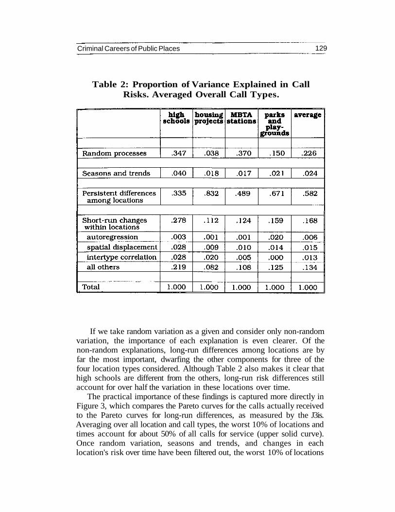
The principal results are shown in Table 2. For each location, similarresults were obtained for crimes, disturbances and services. Thus thetable only shows the average percentage of variation explained over all calltypes. Summarizing the table, we find that
Random variation explains between 4 and 37% of the total variationamong times and locations. It is especially important for locations suchas subway stations and high schools that report fewer calls.
Seasons and trends are relatively unimportant, accounting for only 2to 4% of the total variation.
Long-run differences among locations account for the largest source ofvariation in each case—34 to 83% of the total.
Short-run changes account for 11 to 28% of the total variation. Exceptamong high schools, these changes are not nearly as important aslong-run differences. Relatively little of this variation can be attributedto displacement in time, space and type of call.
Although the random nature of calls for service makes it difficult to identifythe worst locations, most of the variation among times and locations is dueto real differences in risks.
Criminal Careers of Public Places 129
Table 2: Proportion of Variance Explained in CallRisks. Averaged Overall Call Types.
If we take random variation as a given and consider only non-randomvariation, the importance of each explanation is even clearer. Of thenon-random explanations, long-run differences among locations are byfar the most important, dwarfing the other components for three of thefour location types considered. Although Table 2 also makes it clear thathigh schools are different from the others, long-run risk differences stillaccount for over half the variation in these locations over time.
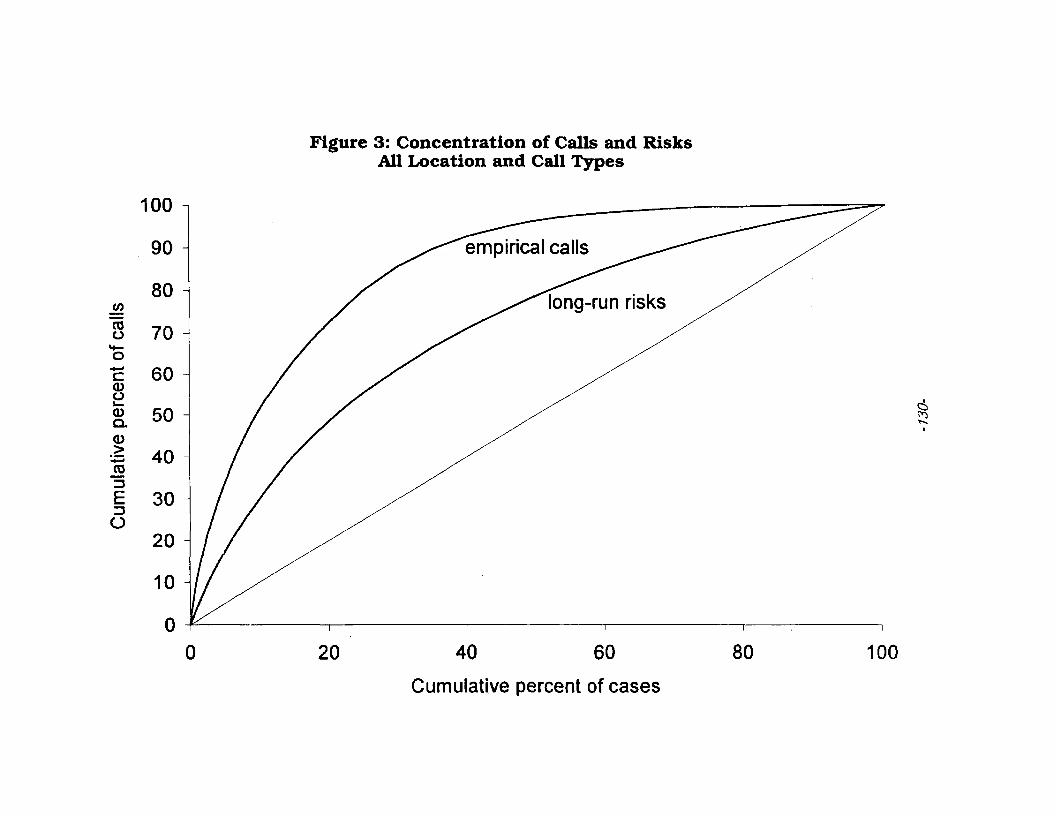
The practical importance of these findings is captured more directly inFigure 3, which compares the Pareto curves for the calls actually receivedto the Pareto curves for long-run differences, as measured by the J3is.Averaging over all location and call types, the worst 10% of locations andtimes account for about 50% of all calls for service (upper solid curve).Once random variation, seasons and trends, and changes in eachlocation's risk over time have been filtered out, the worst 10% of locations
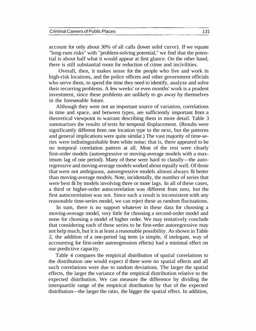
Criminal Careers of Public Places 131
account for only about 30% of all calls (lower solid curve). If we equate"long-runs risks" with "problem-solving potential," we find that the poten-tial is about half what it would appear at first glance. On the other hand,there is still substantial room for reduction of crime and incivilities.
Overall, then, it makes sense for the people who live and work inhigh-risk locations, and the police officers and other government officialswho serve them, to spend the time they need to identify, analyze and solvetheir recurring problems. A few weeks' or even months' work is a prudentinvestment, since these problems are unlikely to go away by themselvesin the foreseeable future.
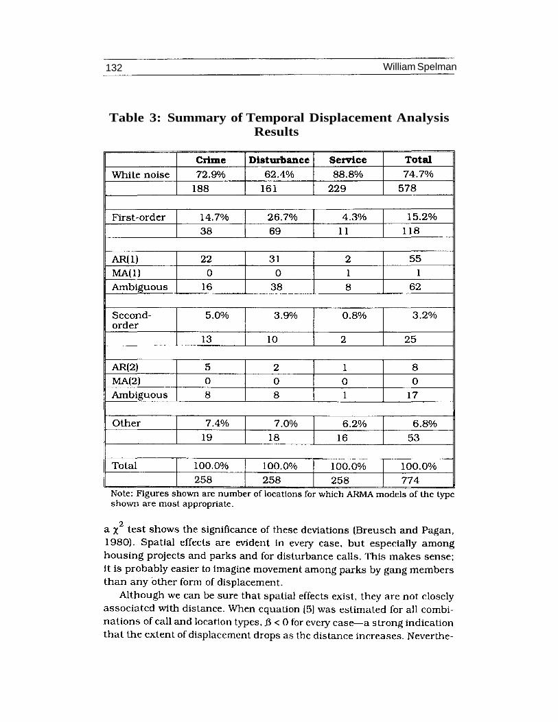
Although they were not an important source of variation, correlationsin time and space, and between types, are sufficiently important from atheoretical viewpoint to warrant describing them in more detail. Table 3summarizes the results of tests for temporal displacement. (Results weresignificantly different from one location type to the next, but the patternsand general implications were quite similar.) The vast majority of time-se-ries were indistinguishable from white noise; that is, there appeared to beno temporal correlation pattern at all. Most of the rest were clearlyfirst-order models (autoregressive or moving-average models with a max-imum lag of one period). Many of these were hard to classify—the auto-regressive and moving-average models worked about equally well. Of thosethat were not ambiguous, autoregressive models almost always fit betterthan moving-average models. Note, incidentally, the number of series thatwere best fit by models involving three or more lags. In all of these cases,a third or higher-order autocorrelation was different from zero, but thefirst autocorrelation was not. Since such a result is inconsistent with anyreasonable time-series model, we can reject these as random fluctuations.
In sum, there is no support whatever in these data for choosing amoving-average model, very little for choosing a second-order model andnone for choosing a model of higher order. We may tentatively concludethat considering each of these series to be first-order autoregressive maynot help much, but it is at least a reasonable possibility. As shown in Table2, the addition of a one-period lag term (a simple, if inelegant, way ofaccounting for first-order autoregression effects) had a minimal effect onour predictive capacity.
Table 4 compares the empirical distribution of spatial correlations tothe distribution one would expect if there were no spatial effects and allsuch correlations were due to random deviations. The larger the spatialeffects, the larger the variance of the empirical distribution relative to theexpected distribution. We can measure the difference by dividing theinterquartile range of the empirical distribution by that of the expecteddistribution—the larger the ratio, the bigger the spatial effect. In addition,
132 William Spelman
Table 3: Summary of Temporal Displacement AnalysisResults

Criminal Careers of Public Places 133
Table 4: Deviations from Random Expectations inSpatial Correlation Distribution
134 William Spelman
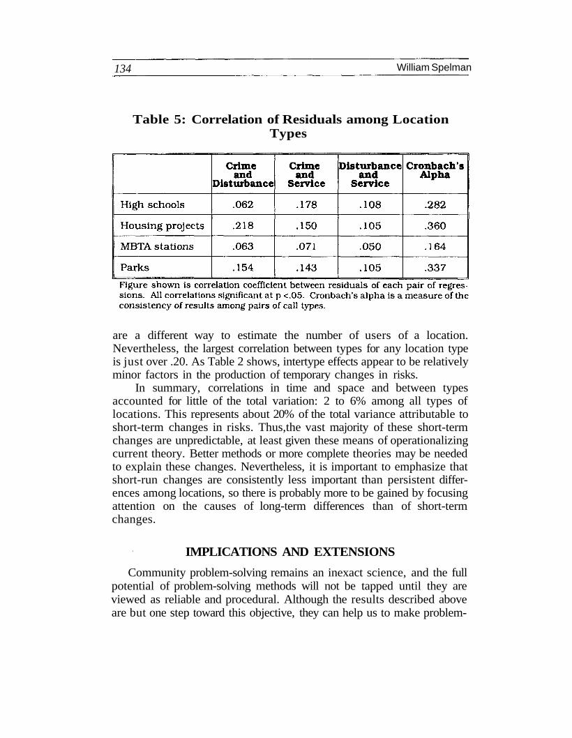
Table 5: Correlation of Residuals among LocationTypes
are a different way to estimate the number of users of a location.Nevertheless, the largest correlation between types for any location typeis just over .20. As Table 2 shows, intertype effects appear to be relativelyminor factors in the production of temporary changes in risks.
In summary, correlations in time and space and between typesaccounted for little of the total variation: 2 to 6% among all types oflocations. This represents about 20% of the total variance attributable toshort-term changes in risks. Thus,the vast majority of these short-termchanges are unpredictable, at least given these means of operationalizingcurrent theory. Better methods or more complete theories may be neededto explain these changes. Nevertheless, it is important to emphasize thatshort-run changes are consistently less important than persistent differ-ences among locations, so there is probably more to be gained by focusingattention on the causes of long-term differences than of short-termchanges.
IMPLICATIONS AND EXTENSIONS
Community problem-solving remains an inexact science, and the fullpotential of problem-solving methods will not be tapped until they areviewed as reliable and procedural. Although the results described aboveare but one step toward this objective, they can help us to make problem-
Criminal Careers of Public Places 135
solving more systematic. Three policy-relevant extensions of this analysisare considered below.
Identifying the Worst Locations. Even if long-run risks are the mostimportant source of variation, for some locations random errors andchanges in risks are also important. So if we identify "high-rate" locationson the basis of only one month of data, we will certainly be fooled some ofthe time.
The simplest solution is to look at calls for service over a longerperiod—three months, six months or a year—and only identify a locationas high rate if it produces a lot of calls throughout the period. As the lengthof the observation period increases, predictive accuracy will improve. Ifthe period is long enough, our predictions will be perfect and accuracy willbe 100%. The problem is that longer time periods are more difficult toprogram into the computer. In some police agencies, computer-aideddispatch system data more than a few months old are simply not available.Thus we must know how much data we need to collect before we canaccurately identify recurring high-risk locations.
The MBTA stations sample provides an appropriate data set for thiskind of thought experiment. Some 37% of the total variation among MBTAstations over time is due to random error—more than any of the otherlocations—so we can be sure that the predictive accuracy for any giventime period will be greater for the others than for this sample. If, forexample, six months is adequate for predicting risks at MBTA stations, itwill be more than adequate for high schools, housing projects and parks.
Figure 4 shows results for three call types and for total calls. For eachcall type, the results are similar. One month of data is sufficient to predictlong-run risks with about 50% accuracy; with two months, accuracy risesto between 60 and 65%; after six months, accuracy is about 80%; and atone year (thirteen 28-day periods), the accuracy is a quite respectable90%. If our only aim is to predict long-run risks for all calls, rather thanfor crimes, disturbances and service calls separately, then we can achieve95% accuracy with only one years' worth of data. Although additional datamay nail down some close calls, and help problem-solvers fine tune theirresource allocations, the differences are unlikely to be critical.
Setting Expectations for Community Problem-solving. If police, neighbor-hood residents, merchants and other users of a location use communityproblem-solving techniques, how well can they be expected to work? Thisquestion is of enormous policy and operational importance. Policymakersare interested in knowing how many eggs we should put in the communityproblem-solving basket; operational personnel need specific objectivesthat can be reasonably achieved and at least a rough idea of when to quit.For example, if problem-solving can realistically reduce crime by, say, 40%


Criminal Careers of Public Places 137
in some location, then line officers and neighborhood organizations err ifthey quit after a 10% reduction—there are many gains left on the table.They also err if they persist after a 38% reduction—there is little left toaccomplish, and they could probably achieve more if they took on adifferent problem.
The only real answer to this question can be obtained through exper-imentation—trying out a wide variety of responses in a wide variety oflocations, and seeing how well they work. Unfortunately, this will takeyears of effort. But we can obtain a rough-cut answer to this question byrephrasing it slightly: What percentage of the long-run differences amonglocations can be attributed to factors beyond the control of problem-solv-ers? If this figure is very high—say, 90%—there is little to be done. On theother hand, if the figure is low, the potential gains are enormous.
The operational problem with answering this question is that it isalmost impossible to get a complete list of the factors that affect risks thatare beyond the control of problem-solvers. Some are well-known. We cancollect data on the number of people who use a location, since more usersmean more opportunities for crime and disorder. We can examine thedemographic characteristics of the users, identifying how many are inhigh-risk groups for offending or victimization, such as young males,single mothers and the poor. In practice, however, we cannot be sure wehave all the relevant variables. This means that any results will probablyunderestimate the variation due to uncontrollable factors, and overesti-mate the importance of the factors controllable by problem-solvers. Keep-ing this significant caveat in mind, let us apply the method to the MBTAstation data.
MBTA stations provide a particularly convenient sample for such ananalysis. The number of people using the stations can be reliably mea-sured from fare-collection data. And, for most locations, we can expectthat the people who use the station are much like those who live in thesurrounding neighborhood. Thus census data can be used to measure thenumber of potential offenders and victims.
When all available data are considered, the best predictors of MBTAstation calls for service turn out to be the total number of station users,the average income of neighborhood residents, whether the station islocated in a commercial area and whether it is on the Orange line, whichruns through the most crime-ridden sections of the city. Other character-istics of the station and its neighborhood added little to our ability toexplain subway crime. These four factors accounted for 55% of the
138 William Spelman
variation among stations, suggesting that roughly half that variation maybe subject to attack by problem-solvers.
Another way of describing the same findings is more direct. The worstfive MBTA stations produce 28% of all calls to subway stations. Whenfactors beyond the control of problem-solvers are accounted for, theyshould have produced only 15%. Thus nearly half of the calls to the worststations could, in theory, be reduced by changing conditions that createcriminal opportunities. If each violent crime costs the victim about$14,000, and each property crime costs about $565 (Cavanagh, 1991;Cohen, 1988), the annual benefits to victims in crime reduction alonecould be as much as $236,000 and $357,000 per year. This does not takeinto account indirect costs of crime, such as avoidance of the subwaysystem, anxiety and fear among those who use it, and the costs ofresponding to these calls.
Although highly speculative, these figures do not seem unreasonable.The more general result certainly seems defensible: factors unique to eachlocation appear to be important determinants of long-run risks; they arepossibly as important as the factors common to all locations. The plausi-bility of the result suggests that the method may help problem-solversguide their resource allocation efforts in the future.
Measuring Effectiveness. If the worst locations cannot be identified withonly one or two months' data, it is clear that changes in long-run risks atthese locations cannot be identified this quickly, either. Random error isliable to swamp any true changes unless rates are measured for severalmonths.
This has two implications for problem-solvers. First, it hampers astrategy of incremental responses. Unless the effect of any given interven-tion is enormous, it will not be possible to make a fast, accurate assess-ment of its effectiveness before trying out another intervention. Moregenerally, this means that many problems will require a long-term com-mitment from the police. Even if officers always play it safe and implementevery response they can think of, they will not succeed. But their failure—when at last it becomes apparent after several months—may suggest otheravenues of approach not obvious from the beginning. Unless the causesof and solutions to a problem are obvious, then, the police will need tocount on an incremental response strategy.
The lag between response and assessment will be even longer if policefind the methods of assessment difficult. The methods most often used forthis purpose—interrupted time-series analysis—are complex and difficultto implement because few computer programs are available.3 If seasonaleffects and sporadic risk changes are relatively unimportant, however, we

Criminal Careers of Public Places 139
can rely on the control chart, a simple means of accounting for randomvariations in time-series data.
Control charts are often used to monitor the incidence of diseases andquality defects (Centers for Disease Control and Prevention, 1986; Mont-gomery, 1991). Briefly, the control chart is simply a plot of the number ofincidents reported over time, with the average value and expected upperand lower ranges drawn in for comparison. So long as the time-series stayswithin the upper and lower bounds, the problem is in "statistical control"—not getting better, but not getting worse, either (Deming, 1986). If thetime-series drops below the lower bound after an intervention has beenimplemented,then the problem-solvers can be reasonably certain that theyhave ameliorated the problem.
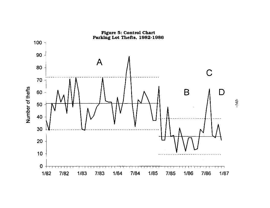
In Newport News, VA, a patrol sergeant used a control chart to monitorburglaries from automobiles parked near a large factory (Eck and Spel-man, 1987). As shown in Figure 5, the number of burglaries had beenclose to statistical control for the three years preceding the intervention(labeled A on the figure). In March 1985, two gangs of youthful burglarswere broken up, and in the next month the number of burglaries wentbelow the lower bound for the first time on record. It stayed there forseveral months, establishing a new level with a lower average (B). Aboutone year after the initial intervention, the number of burglaries rose abovethe new upper bound, signaling that the system had changed again (Q.Investigation showed that a pair of high-rate juvenile offenders hadentered the area, and the burglary rate went down after they were arrestedand incapacitated (D).
As this example demonstrates, the control chart can be an invaluableassessment tool. The officers assigned to this problem could show withintwo months that their efforts were having an effect (in part because theeffect was so large). The chart also showed when conditions changed,making an early response possible. Finally, the chart fulfills some admin-istrative objectives. Because they are easy to use, control charts can bemaintained by operational personnel. This sustains the focus on resultsand improves the link between the line officers' actions and the conse-quences of their actions for the public.
The classic control chart only aims to separate random variations fromlong-run averages, and upper and lower bounds are set under the assump-tion that there are no seasonal or trend effects or short-run changes inrisks. As shown above, these are unrealistic assumptions for most publicplaces (although they were fairly realistic for the auto burglaries problem).They are particularly unrealistic for the housing project series, for whichrandom processes explain only 4% of the variation but seasons, trendsand other short-run changes explain 13%. When these assumptions were
Criminal Careers of Public Places 141
applied to the 105 housing project series (crime, disturbance, and servicecall time-series for each of 35 projects), the results were predictablydisastrous. For most series, some months lay well above the bounds, eventhough the long-term risks remained constant. The underlying distribu-tion was more skewed than the Poisson for all series.
Use of a control chart with inappropriate bounds would be misleading,but the skewed nature of the distribution suggests an effective adjust-ment. There are reasons to believe that temporary changes in risks shouldbe multiplicative in nature (Spelman, 1992), thus the distribution ofunderlying risks for each series should be roughly logNormal. Althoughrandom deviations about these (changing) underlying risks add to thevariability, Table 2 shows that temporary changes are roughly three timesas important as random deviations in explaining the variability withinthese series. So the number of calls reported over time for any givenlocation should be roughly logNormal-distributed. Thus, appropriatebounds can be set by using the following procedure:
1. Estimate the mean of the empirical series through the usualmethods.
2. Take the logarithm of all cases, and estimate the mean andstandard deviation of the log distribution.
3. Multiply the log standard deviation by 3.0 (as usual), and add itto and subtract it from the mean of the log distribution. These arethe appropriate control limits for a logNormal distribution.
4. Take the exponent of the upper and lower bounds to form boundsfor the control chart.
This structures the control chart to screen out random deviations plusshort-term changes in underlying risks that are like those found in therecent past. If a new program or policy is effective enough to reduce risksby more than these amounts, the control chart should correctly reflect it.
When upper and lower bounds are set in this way, 95% of time-seriesin the Boston calls-for-service data set are consistently within bounds:
• 76% fit the control chart perfectly (that is, they were in controlthroughout the four-year period);
• 19% had more points near the lower bounds than expected, butdid not go below the bounds; and
• only 5% included months that went outside the upper or lowerbounds.
Since this would happen in about 5% of the series just by chance,4 thecontrol charts appeared to be working perfectly. Thus the Boston data

142 William Spelman
confirm that control charts can work on calls-for-service data in a widevariety of locations. By adopting this simple and effective way to monitorproblems and assess the impact of responses, line officers can makesophisticated statistical judgments.
CONCLUSION
The promise of sitting ducks, ravenous wolves and dens of iniquity isthat we can accomplish a lot by focusing our efforts on a few. In theory,we can rehabilitate, deter or at least incapacitate a few very dangerousoffenders; we can help especially vulnerable victims to avoid crime anddefend themselves; and we can solve problems at especially dangerouslocations, reducing them without displacing them. As with dangerousoffenders and vulnerable victims, some of this promise is lost upon closeexamination. Much of the concentration of crime among locations is dueto random and temporary fluctuations that are beyond the power of thepolice and the public to control reliably.
On the other hand, there is much left to be gained through communityproblem-solving. Among public places, at least, the worst 10% of locationsreliably account for some 30% of all calls. The results described abovesuggest that crime, disturbances and other calls for service can be reducedby something like 50% in the most dangerous locations, simply by focusingon the unique characteristics of those locations that create opportunitiesfor crime and disorder. It remains to be seen whether we can develop thetools to analyze and respond to these problems adequately. But thepotential benefits remain vast and worthy of further study.
NOTES1. Accuracy is defined here as the squared correlation between the number
of calls received during the short-run period and the long-run expectationsfor each location, averaged over all locations.
2. In general, this is referred to as the problem of "left-out variable error."For more information, see Judge et al., 1985.
3. For example, the most widely used statistical package, SAS, has onlyrecently made an interrupted time-series analysis program available as astandard option (SAS Institute, 1991). No such program is as yet availableon SPSS.
Criminal Careers of Public Places 143
4. Bounds were set so that 0.1% of observations would go beyond thebounds due to random variation, so the expected number of beyond-boundobservations is 52 x .001 = .052 per series. Thus, 5.2% of the series shouldinclude one or more beyond-bounds observations.
REFERENCESBerk, R.A., D.M. Hoffman, J.E. Maki, D. Rauma and H. Wong (1979).
"Estimation Procedures for Pooled Cross-sectional and Times-seriesData." Evaluation Quarterly 3:385-410.
Blumstein, A., J. Cohen, J.A. Roth and C.A. Visher (eds.) (1986). CriminalCareers and "Career Criminals." Washington, DC: National AcademyPress.
Box, G.E.P. and G.M. Jenkins (1976). Time-series Analysis: Forecasting andControl. San Francisco, CA: Holden-Day.
Breusch, T.S. and A.P. Pagan (1980). The LaGrange Multiplier Test and ItsApplications to Model Specification in Economics." Review of EconomicStudies 47:239-254.
Cavanagh, D.P. (1991). A Cost-Benefit Analysis of Prison Cell Constructionand Alternative Sanctions. Cambridge, MA: BOTEC Analysis Corp.
Centers for Disease Control and Prevention (1986). Principles of Epidemiol-ogy: Disease Surveillance. Manual 5, Self-Study Course 3030-G. At-lanta, GA: author.
Chaiken, J.M. and M. Chaiken (1982). Varieties of Criminal Behavior. SantaMonica, CA: Rand.
Clarke, R.V. and D.L. Weisburd (1992). "On the Distribution of Deviance."In: D.M. Gottfredson and R.V. Clarke (eds.), Policy and Theory inCriminal Justice. Aldershot, UK: Avebury.
Cohen, M. (1988). "Pain, Suffering, and Jury Awards: A Study of the Costof Crime to Victims." Law and Society Review 22:537-555.
Cohen, L.E. and M. Felson (1979). "Social Change and Crime Rate Trends:A Routine Activity Approach." American Sociological Review 44:588-608.
Deming, W.E. (1986). Out of the Crisis. Cambridge, MA: MIT Press.Eck.J.E. and W. Spelman (1987). Problem Solving: Problem-Oriented Polic-
ing in Newport News. Washington, DC: Police Executive ResearchForum.
Fienberg, S.E. (1980). "Statistical Modeling in the Analysis of RepeatVictimization." In: S.E. Fienberg and A.J. Reiss, Jr. (eds.), Indicatorsof Crime and Criminal Justice: Quantitative Studies. Washington, DC:U.S. Government Printing Office.
Goldstein, H. (1990). Problem-Oriented Policing. New York, NY: McGraw-Hill.

144 William Spelman
Greene, J.R. and S.D. Mastrofski (eds.) (1988). Community Policing: Rhetoricor Reality? New York, NY: Praeger.
Horney, J. and I.H. Marshall (1991). "Measuring Lambda Through Self-Re-ports." Criminology 29:401-425.
Judge, G.G., W.E. Griffiths, R.C. Hill, H. Luetkepohl and T.C. Lee (1985).The Theory and Practice of Econometrics. New York, NY: John Wiley &Sons.
McCleary, R. and R.A. Hay, Jr. (1980). Applied Time Series Analysis for theSocial Sciences. Beverly Hills, CA: Sage.
Mande. M. J. and K. English (1988). Individual Crime Rates of ColoradoPrisoners. Denver, CO: Division of Criminal Justice, Colorado Depart-ment of Public Safety.
Montgomery, D.C. (1991). Introduction to Statistical Quality Control. NewYork, NY: John Wiley & Sons.
Nelson, J. F. (1984). "Multiple Victimization in American Cities: A StatisticalAnalysis of Rare Events." American Journal of Sociology 85:870-891.
Pierce, G.L., S. Spaar and L.R. Briggs (1986). The Character of Police Work:Strategic and Tactical Implications. Boston, MA: Center for AppliedSocial Research, Northeastern University.
Reiss, A.J., Jr. (1980). "Victim Proneness in Repeat Victimization by Typeof Crime." In: S.E. Fienberg and A.J. Reiss, Jr. (eds.), Indicators ofCrime and Criminal Justice: Quantitative Studies. Washington, DC:U.S. Government Printing Office.
SAS Institute (1991). SAS/ETS User's Guide (version 6). Cary, NC: author.Sherman, L.W., P.R. Gartin and M.E. Buerger (1989). "Hot Spots of
Predatory Crime: Routine Activities and the Criminology of Place."Criminology 27:27-55.
Spelman, W. (1992). Criminal Careers of Public Places. Final Report to theU.S. National Institute of Justice. Austin, TX: LBJ School of PublicAffairs, University of Texas at Austin.
Srivistava, V.K. and D.E.A. Giles (1987). Seemingly Unrelated RegressionEquations Models: Estimation and Inference. New York, NY: MarcelDekker.
Stimson, J.A. (1985). "Regression in Space and Time: A Statistical Essay."American Journal of Political Science 29:914-947.
Zedlewski, E.F. (1987). Making Confinement Decisions. Research in Brief.Washington, DC: National Institute of Justice.
Zellner, A. (1962). "An Efficient Method of Estimating Seemingly UnrelatedRegression Equations and Tests for Aggregation Bias." Journal of theAmerican Statistical Association 57:348-368.