Crime in St. Louis Cityin 2011

David AdamsJohn Fields

Leticia GarciaShawn KainadyChris SchaeferTravis Tatum

Our Mission

Mission: Use statistics and data sets to predict the number and location of unlawful homicides in St. Louis City in 2011.

Concern: The CQ Press released the results of a study that named St. Louis, MO, as the most dangerous city in the United States. (chosen over lovely vacation spots like Detroit, MI; Camden, NJ; and Oakland, CA)

2010 population: 319,294

No. of neighborhoods: 79

Homicide history

Year 2005 2006 2007 2008 2009 2010

No. of Homicides 130 126 134 162 142 143

St. Louis City Facts

Homicides can be predicted rather accurately by analyzing environmental variables.

Example: Large number of bars in a particular neighborhood might lead to increase in drunk driving.

No foreseen catastrophic event (e.g., federal government shutting down March 4)

Murder is bad

Assumptions

Homicide rates are affected by variables such as income and education as well as both violent and non-violent crimes that do not result in homicide.

By knowing where there are deficiencies in education, we can predict where there will also be more homicides.

Hypothesis

 Crime stats collected from StL Metro Police Dept (

http://www.slmpd.org/crime_stats.html)

Data collected and analyzed by neighborhood

Data also collected from 2000 Census (http://stlcin.missouri.org/citydata/newdesign/index.cfm)

 

Data Mining

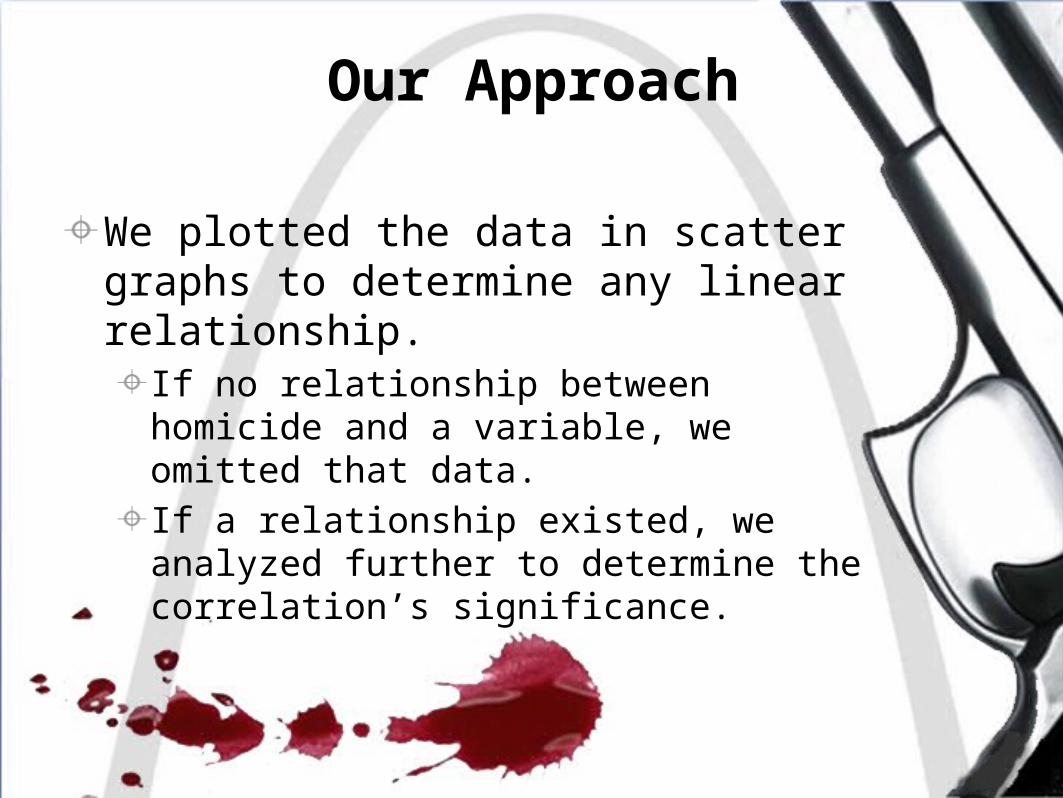
We plotted the data in scatter graphs to determine any linear relationship.

If no relationship between homicide and a variable, we omitted that data.

If a relationship existed, we analyzed further to determine the correlation’s significance.

Our Approach

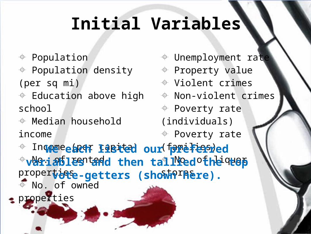
Population Population density (per sq mi) Education above high school Median household income Income (per capita) No. of rented properties No. of owned properties

Unemployment rate Property value Violent crimes Non-violent crimes Poverty rate (individuals) Poverty rate (families) No. of liquor stores

Initial Variables

We each listed our preferred variables and then tallied the top vote-getters (shown here).

Regressions

We used Minitab to compare homicides to our initial variables to determine the greatest correlations.

We discovered some very interesting correlations.

R^2 P-Value Y-intercept SlopeViolent Crimes 0.69 1.88E-21 -0.1633 0.0207Non-Violent Crimes 0.78 3.76E-27 -0.01856 0.4019Income 0.17 0.000213 3.714 -0.00012Property Value 0.18 0.000113 3.3366 -2.20E-05Property Rented 0.002 0.65 2.09 -0.00536Property Owned 0.003456 0.609 1.514 0.006101Unemployment 0.0376 0.088 1.32 0.031Poverty Rate Individual 0.077 0.013662 0.6274 0.041Poverty Rate Family 0.071098 0.018285 0.84672 0.0398Liquor Stores 0.23437 7.10E-06 0.8987 0.9736Population 0.08 0.011897 1.0217 0.000171Population Density 0.05 0.047 0.7756 0.000147High school Education 0.28 5.66E-07 4.952 -0.07345Median Household Income 0.16 0.000275 4.33 -9.60E-05

Results of Regressions

Final Variables

Population Population density (per sq mi) Education above high school Median household income Income (per capita)

Property value No. of violent crimes No. of non-violent crimes Poverty rate (individuals) Poverty rate (families) No. of liquor stores

We used the resulting 11 variables in our final predictions.

Variable with the greatest degree of correlation (most probable) with homicide is Non-Violent Crimes.

R2 value = .78 (highest)

P-value = 3.76E-27 (lowest)

Our Results

0 200 400 600 800 1000120014001600180020000

1

2

3

4

5

6

7

8

9

10

Non-Violent Crimes

Crime of Property

# of Non-Violent Crimes

# N

um

ber

of

Mu

rder

s

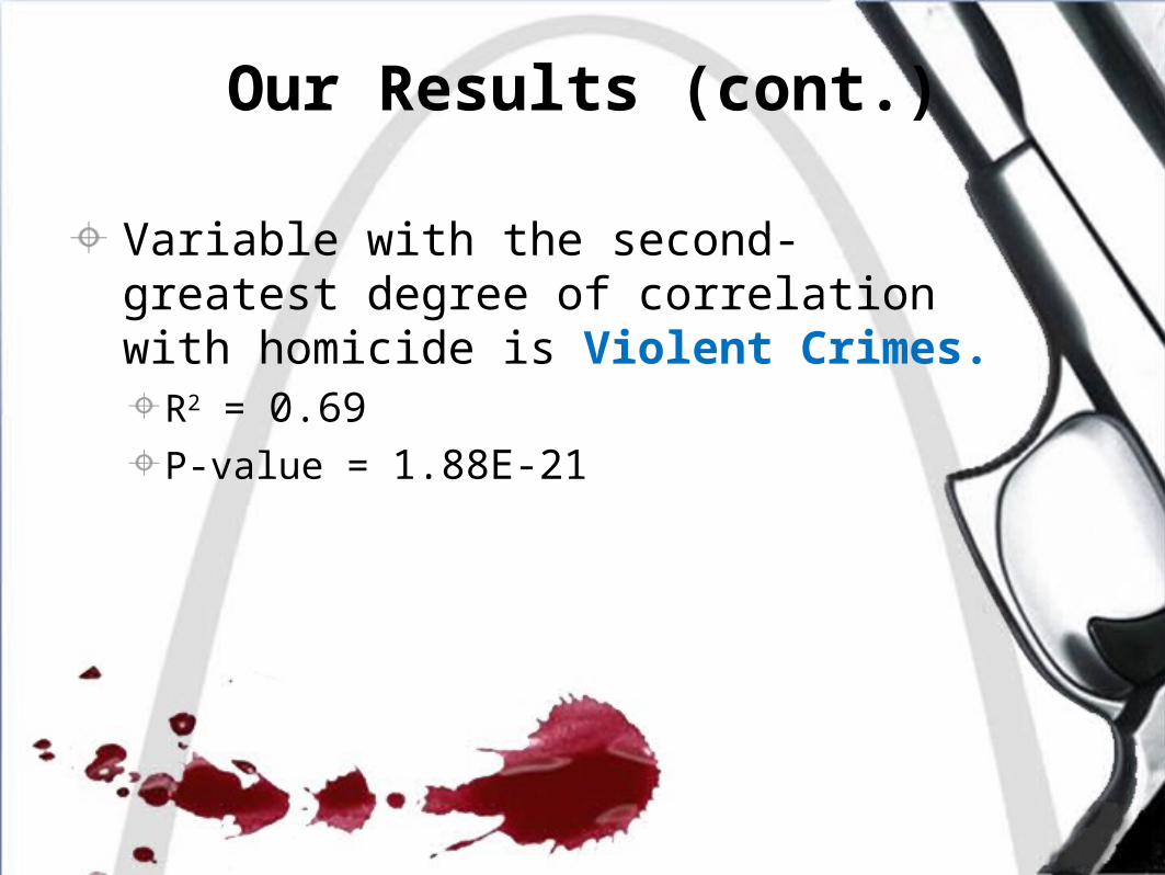
Variable with the second-greatest degree of correlation with homicide is Violent Crimes.

R2 = 0.69P-value = 1.88E-21

Our Results (cont.)

0 50 100 150 200 250 300 350 400 4500

123

456

789

10

Violent Crimes

Crime of person

Number of Violent Crimes

# o

f M

urd

ers

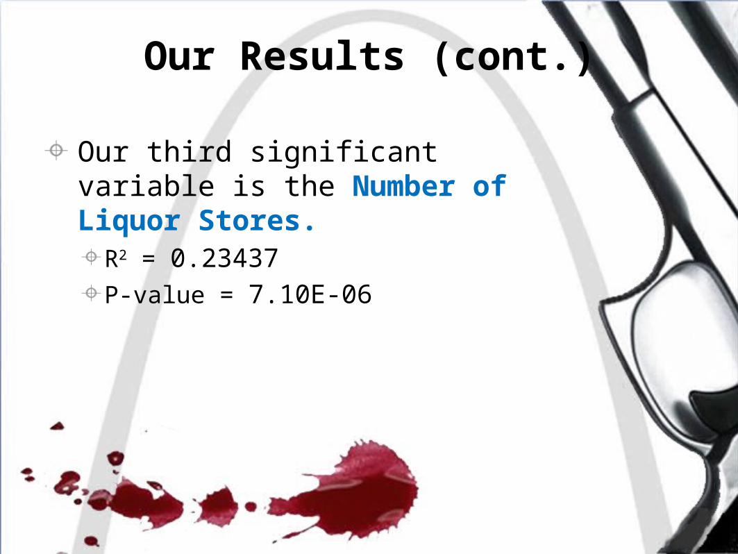
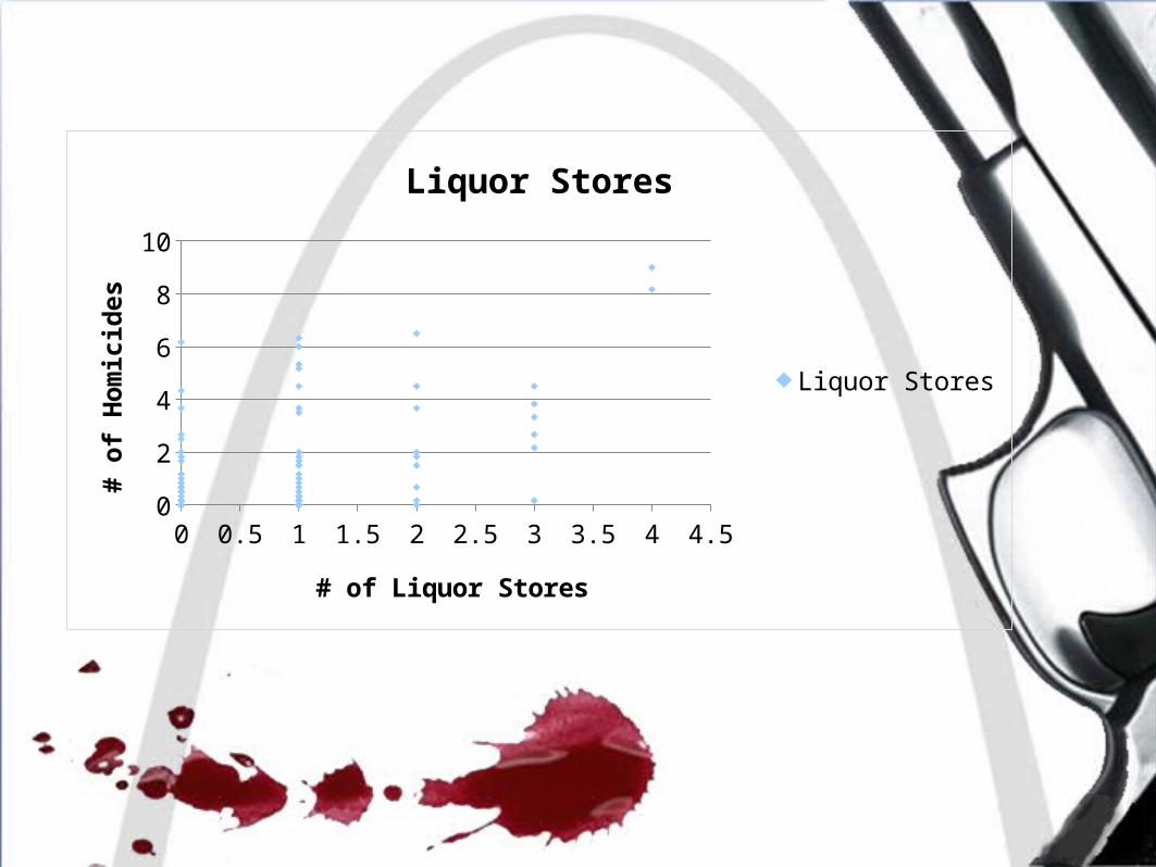
Our third significant variable is the Number of Liquor Stores.

R2 = 0.23437P-value = 7.10E-06

Our Results (cont.)

0 0.5 1 1.5 2 2.5 3 3.5 4 4.50

2

4

6

8

10

Liquor Stores

Liquor Stores

# of Liquor Stores

# o

f H

om

icid

es

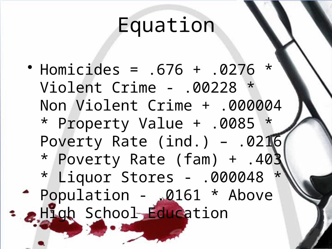
Equation

• Homicides = .676 + .0276 * Violent Crime - .00228 * Non Violent Crime + .000004 * Property Value + .0085 * Poverty Rate (ind.) – .0216 * Poverty Rate (fam) + .403 * Liquor Stores - .000048 * Population - .0161 * Above High School Education

Using 2000 Census data it is predicted that JeffVanderLou will have the most Homicides in 2011.

Our Results (cont.)

NEIGHBORHOOD 2005 2006 2007 2008 2009 2010Forecasted 2011

Jeff Vanderlou 5 4 10 13 10 7 8.3

Wells-Goodfellow 9 4 14 10 11 6 8.16

Dutchtown 4 2 2 6 3 5 7.04The Greater Ville 10 9 4 5 5 5 5.88

O'Fallon 5 9 7 9 3 6 5.23

Acad emy 2 3 4 6 3 2 4.37Gravois Park 2 0 5 3 1 4 4.31Baden 7 5 4 6 7 7 4.27

Walnut Park East 13 5 4 3 3 3 4.24Hamilton Heights 4 2 8 6 4 3 4.15West End 3 8 1 5 5 4 3.81

Number of homicides: 8.3

Location of homicides: JeffVanderLou

Total Forecasted City of St. Louis Homicides: 142.10

Our Predictions

Conclusion

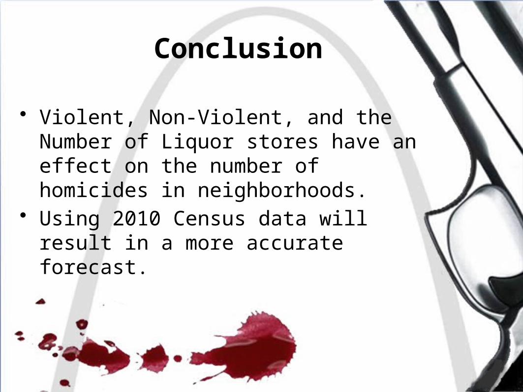
• Violent, Non-Violent, and the Number of Liquor stores have an effect on the number of homicides in neighborhoods.

• Using 2010 Census data will result in a more accurate forecast.

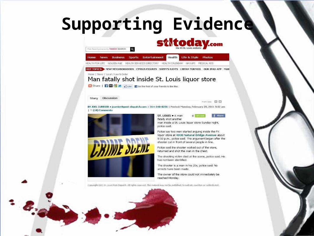
Supporting Evidence

Thank You!