creo.2 crank mechanism analysis - mycourses · mec-e1060 machine design kaur jaakma 2016 creo.2 3 /...

CREO.2 – CRANK MECHANISM ANALYSIS

Figure 1: Analyzed mechanism and a graph.

MEC-E1060 Machine Design Kaur Jaakma 2016

Creo.2

2 / 24

Learning Targets

In this exercise you will learn:

to create family table parts

to create multi-body assemblies

to perform mechanism simulation

to plot results.

In this exercise a crank mechanism similar to Mathcad.1 and Mathcad.2 exercises is created and

analyzed. With Mathcad we defined the force balance equations and solved those manually. With

Creo, we create equivalent geometry and use Multi-Body Simulation (MBS) tools to solve force

balance cases and to plot results.

The used program is PTC Creo 3.0 M050, but the method also works with older versions.


Creo.2

3 / 24

Getting Started

Start Creo Parametric 3.0 M050 from Windows start menu. First thing to do is to define working

directory (e.g. directory that Creo used for temporally files and to store results). Select Select

Working Directory ( , Data group) and create a new folder (RMB, New Folder) for Creo (for ex.

Z:\Creo\).

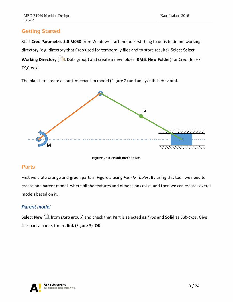
The plan is to create a crank mechanism model (Figure 2) and analyze its behavioral.

Figure 2: A crank mechanism.

Parts

First we crate orange and green parts in Figure 2 using Family Tables. By using this tool, we need to

create one parent model, where all the features and dimensions exist, and then we can create several

models based on it.

Parent model

Select New ( , from Data group) and check that Part is selected as Type and Solid as Sub-type. Give

this part a name, for ex. link (Figure 3). OK.


Creo.2

4 / 24

Figure 3: Creating a new part called link.

Extrude

Select Extrude ( , from Shapes group) and select FRONT plane from the graphical area (or from the

Model Tree in the left). A Sketch mode appears. Using Circle ( , from Sketching group), create two

equal-sized circles, starting from the center of the sketch (dashed lines). When creating the second

one, Creo will offer R (Equal Radii) constraint when the size of the second circle is about the same as

the first one’s (Figure 4).

Figure 4: Creating second circle to the right, program offering R (Equal Radii).


Creo.2

5 / 24

Then, using Line ( , from Sketching group) create horizontal line starting from the intersection of the

leftmost circle and Y-axis (Figure 5) and attach the line to the rightmost circle using T (Tangent

Entities) as seen in Figure 5. Accept with MMB.

Figure 5: On left: selecting starting point. On right: selecting end point.

Using the same method, create another line on the bottom. You can close the tool by pressing MMB

second time (first time ends the current line, second closes the tool).

Using Delete Segment ( , from Editing group), remove the unnecessary arcs from the sketch by

holding LMB and moving mouse cursor over removable lines (Figure 6). MMB to close the tool.

Figure 6: Removing arcs (highlighted in green), tool path highlighted in red.


Creo.2

6 / 24

Next, using Normal ( , from Dimension group), create a dimension by first selecting the upper

horizontal line, then lower horizontal line and then pressing MMB between them (Figure 7). Close the

tool with MMB.

Figure 7: Both horizontal lines selected and MMB pressed.

Give 10 as a height and 100 as the width (double-click the grey dimension to edit it) as seen in Figure

8. You can move the location of the dimension by selecting it and moving around.

Figure 8: Dimensions created and updated.

By default, Creo doesn’t create datum axes on the center of arcs. We need to have those, so select

Point ( ) from Datum group (there are two points, one in Sketching group is only visible within the

sketch) and place points in the center of the arcs (Figure 9).

Figure 9: Datum point created in the center of the arc.


Creo.2

7 / 24

When ready, accept the sketch by selecting OK ( , from Close group) or holding RMB and selecting

OK.

Give 10 as the length of the extrude and accept the feature ( or MMB). Select Extrude 1 from the

Model Tree, RMB and select Rename. Give base as a name (all user defined names will be in

UPPERCASE). It is a good practice to rename features and give them meaningful names. It helps a lot

when models are big and some changes are needed.

First Hole

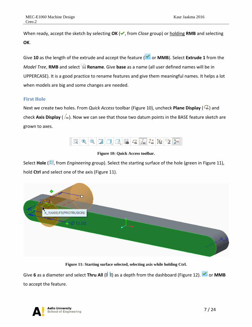
Next we create two holes. From Quick Access toolbar (Figure 10), uncheck Plane Display ( ) and

check Axis Display ( ). Now we can see that those two datum points in the BASE feature sketch are

grown to axes.

Figure 10: Quick Access toolbar.

Select Hole ( , from Engineering group). Select the starting surface of the hole (green in Figure 11),

hold Ctrl and select one of the axis (Figure 11).

Figure 11: Starting surface selected, selecting axis while holding Ctrl.

Give 6 as a diameter and select Thru All ( ) as a depth from the dashboard (Figure 12). or MMB

to accept the feature.


Creo.2

8 / 24

Figure 12: Dashboard and selecting Thru All from the drop-down list.

Second hole

We can use the same method as previously to create a second hole. But we can also use copy-paste

to create another hole. Select Hole 1 from the model tree and press Ctrl + C. Then, select Paste

Special ( ) from Operations group (Figure 13).

Figure 13: Selecting Paste Special.

Check the option Advanced reference configuration and press OK. A new window appears. This

window lists all references that hole feature has (starting surface and placement axis). Select the AXIS

from the list and select another axis in the model. Press to accept the new copied feature.

Datum points

Next we create several datum points for working as measurement points for mechanical simulation.

Select Point ( , from Datum group). Ensure that Plane Display ( ) is off and Axis Display ( ) is on

in the Quick Access toolbar. Then, select one of the axes, hold Ctrl and select one of the main surfaces

in the part (Figure 14). This creates a point in the cross-section of axis and plane.


Creo.2

9 / 24

Figure 14: Axis selected (light green), selecting surface (green) while holding Ctrl.

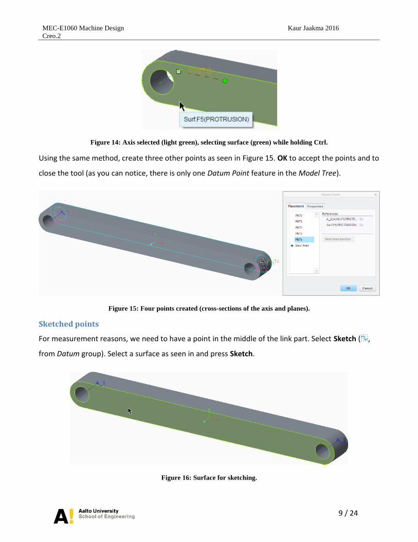
Using the same method, create three other points as seen in Figure 15. OK to accept the points and to

close the tool (as you can notice, there is only one Datum Point feature in the Model Tree).

Figure 15: Four points created (cross-sections of the axis and planes).

Sketched points

For measurement reasons, we need to have a point in the middle of the link part. Select Sketch ( ,

from Datum group). Select a surface as seen in and press Sketch.

Figure 16: Surface for sketching.


Creo.2

10 / 24

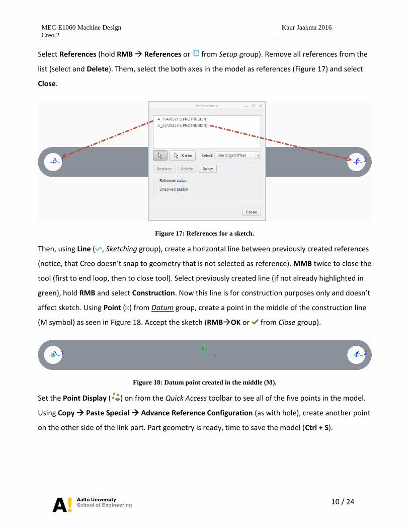
Select References (hold RMB References or from Setup group). Remove all references from the

list (select and Delete). Them, select the both axes in the model as references (Figure 17) and select

Close.

Figure 17: References for a sketch.

Then, using Line ( , Sketching group), create a horizontal line between previously created references

(notice, that Creo doesn’t snap to geometry that is not selected as reference). MMB twice to close the

tool (first to end loop, then to close tool). Select previously created line (if not already highlighted in

green), hold RMB and select Construction. Now this line is for construction purposes only and doesn’t

affect sketch. Using Point ( ) from Datum group, create a point in the middle of the construction line

(M symbol) as seen in Figure 18. Accept the sketch (RMBOK or from Close group).

Figure 18: Datum point created in the middle (M).

Set the Point Display ( ) on from the Quick Access toolbar to see all of the five points in the model.

Using Copy Paste Special Advance Reference Configuration (as with hole), create another point

on the other side of the link part. Part geometry is ready, time to save the model (Ctrl + S).


Creo.2

11 / 24

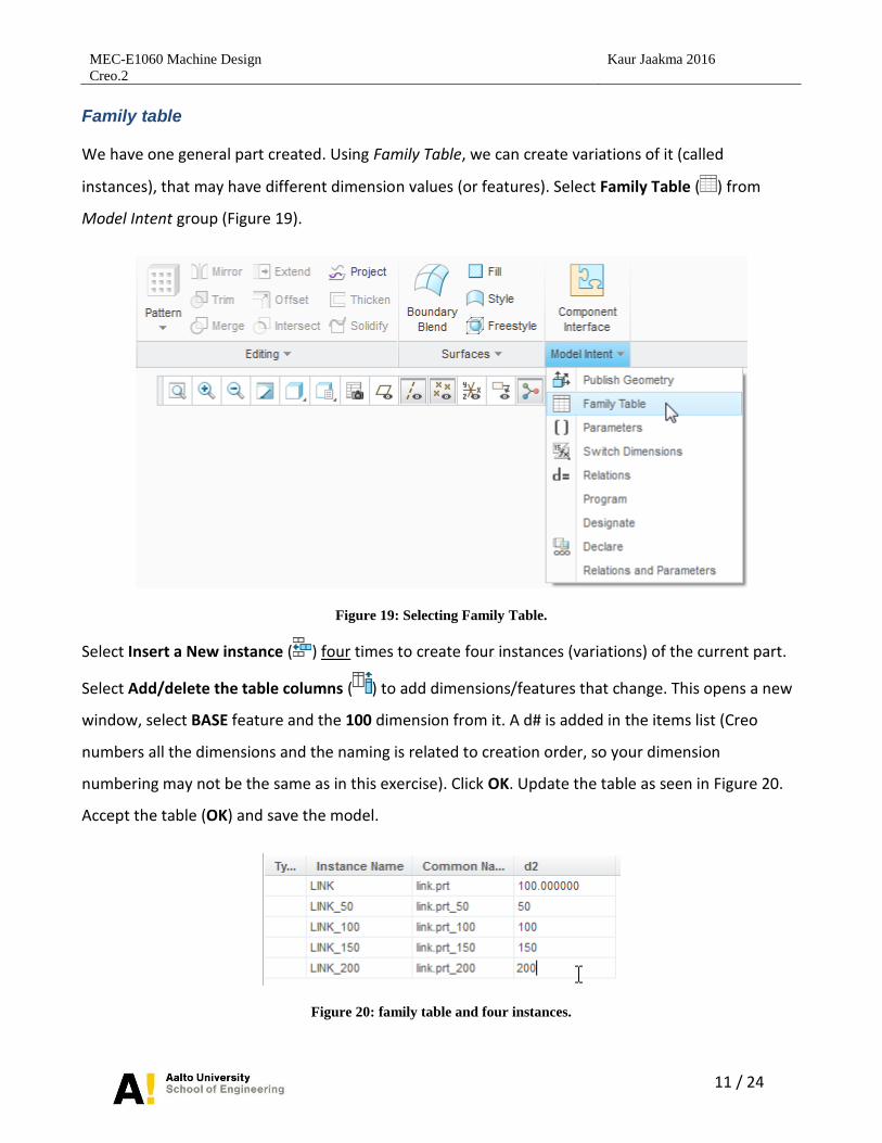
Family table

We have one general part created. Using Family Table, we can create variations of it (called

instances), that may have different dimension values (or features). Select Family Table ( ) from

Model Intent group (Figure 19).

Figure 19: Selecting Family Table.

Select Insert a New instance ( ) four times to create four instances (variations) of the current part.

Select Add/delete the table columns ( ) to add dimensions/features that change. This opens a new

window, select BASE feature and the 100 dimension from it. A d# is added in the items list (Creo

numbers all the dimensions and the naming is related to creation order, so your dimension

numbering may not be the same as in this exercise). Click OK. Update the table as seen in Figure 20.

Accept the table (OK) and save the model.

Figure 20: family table and four instances.


Creo.2

12 / 24

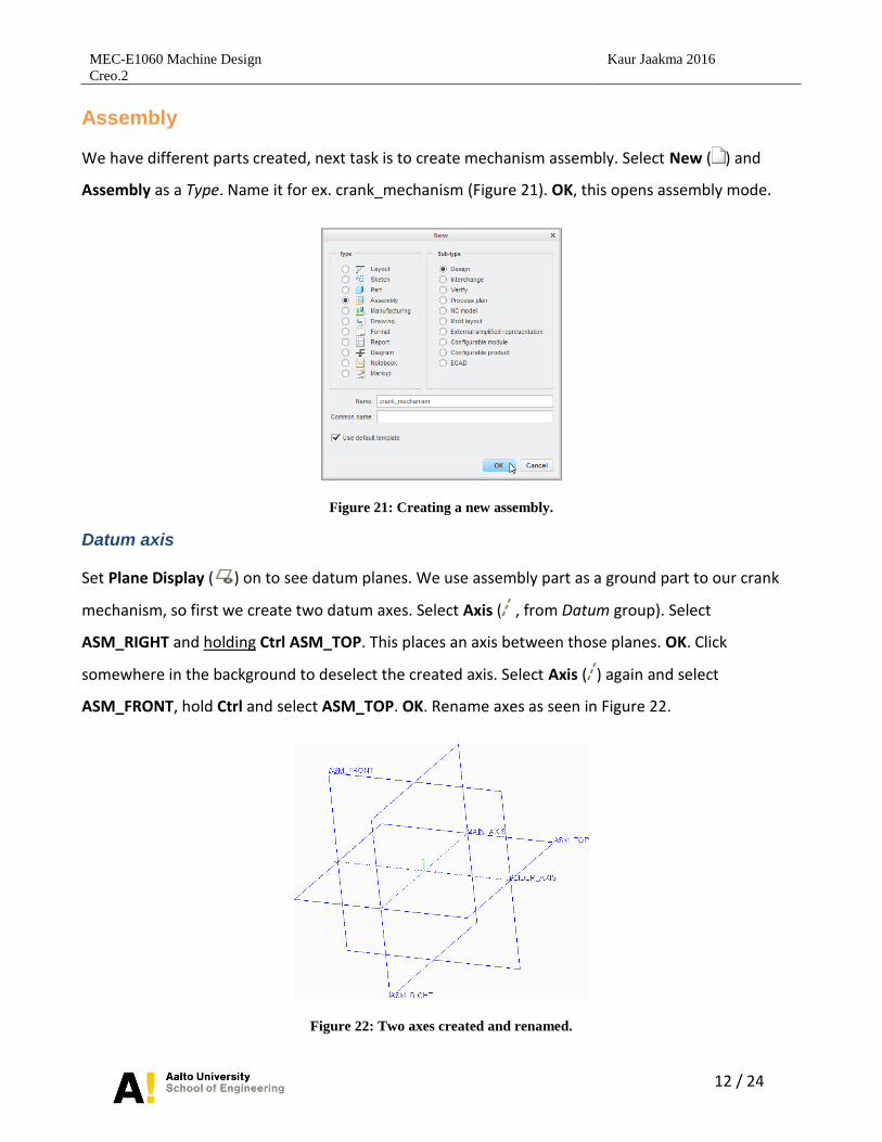
Assembly

We have different parts created, next task is to create mechanism assembly. Select New ( ) and

Assembly as a Type. Name it for ex. crank_mechanism (Figure 21). OK, this opens assembly mode.

Figure 21: Creating a new assembly.

Datum axis

Set Plane Display ( ) on to see datum planes. We use assembly part as a ground part to our crank

mechanism, so first we create two datum axes. Select Axis ( , from Datum group). Select

ASM_RIGHT and holding Ctrl ASM_TOP. This places an axis between those planes. OK. Click

somewhere in the background to deselect the created axis. Select Axis ( ) again and select

ASM_FRONT, hold Ctrl and select ASM_TOP. OK. Rename axes as seen in Figure 22.

Figure 22: Two axes created and renamed.


Creo.2

13 / 24

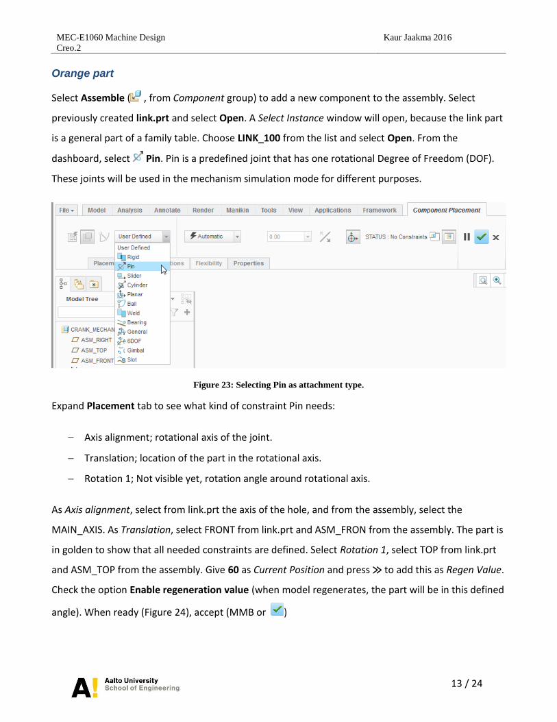
Orange part

Select Assemble ( , from Component group) to add a new component to the assembly. Select

previously created link.prt and select Open. A Select Instance window will open, because the link part

is a general part of a family table. Choose LINK_100 from the list and select Open. From the

dashboard, select Pin. Pin is a predefined joint that has one rotational Degree of Freedom (DOF).

These joints will be used in the mechanism simulation mode for different purposes.

Figure 23: Selecting Pin as attachment type.

Expand Placement tab to see what kind of constraint Pin needs:

Axis alignment; rotational axis of the joint.

Translation; location of the part in the rotational axis.

Rotation 1; Not visible yet, rotation angle around rotational axis.

As Axis alignment, select from link.prt the axis of the hole, and from the assembly, select the

MAIN_AXIS. As Translation, select FRONT from link.prt and ASM_FRON from the assembly. The part is

in golden to show that all needed constraints are defined. Select Rotation 1, select TOP from link.prt

and ASM_TOP from the assembly. Give 60 as Current Position and press ≫ to add this as Regen Value.

Check the option Enable regeneration value (when model regenerates, the part will be in this defined

angle). When ready (Figure 24), accept (MMB or )


Creo.2

14 / 24

Figure 24: First part added and rotational angle defined.

Green part

Next we add the second part to the assembly (green in Figure 2). Select Assemble ( , from

Component group) and select link.prt LINK_200. Select Pin as joint and assemble as seen in

Figure 25 (you can hide 3D dragger by selecting ).

Figure 25: Hole axes constrained and two surfaces added together (arrows).


Creo.2

15 / 24

Select New Set to define another joint. Select General as a type. From the assembly, select

SLIDER_AXIS and from the part, a point (Figure 26).

Figure 26: An axis (SLIDER_AXIS) and a point (PNT2 in this case) added together.

Now all joints are defined, accept (MMB).

You can use Drag Components ( , from Component group) to select a entity and drag mechanism

around to see how it works. When ready, press Ctrl + G to regenerate model to the default position.

Save the model.

Multi-body Simulation

Select Applications tab and Mechanism ( , from Motion group) to start using mechanism analyses

mode. Here you can see which kind of joint your model has (Figure 27). In our case, two rotational

joints (an arrow and arc over it) and one translation general joint (arrow towards Z). Click Highlight

Bodies ( , Bodies group) to see different moving bodies in the assembly.


Creo.2

16 / 24

Figure 27: A crank mechanism. Joints highlighted in green.

Needed torque

First we calculate the needed torque to hold the mechanism still in 60 deg angle. We calculated

already the needed torque in Methcad.1 and .2 exercises (58.84 Nmm), so now we check that

mechanism simulation give similar result.

The simulation process includes:

Define a servo motor that stays in the right angle.

Define measurement.

Define dynamic analysis including gravity.

Run simulation.

Plot result.


Creo.2

17 / 24

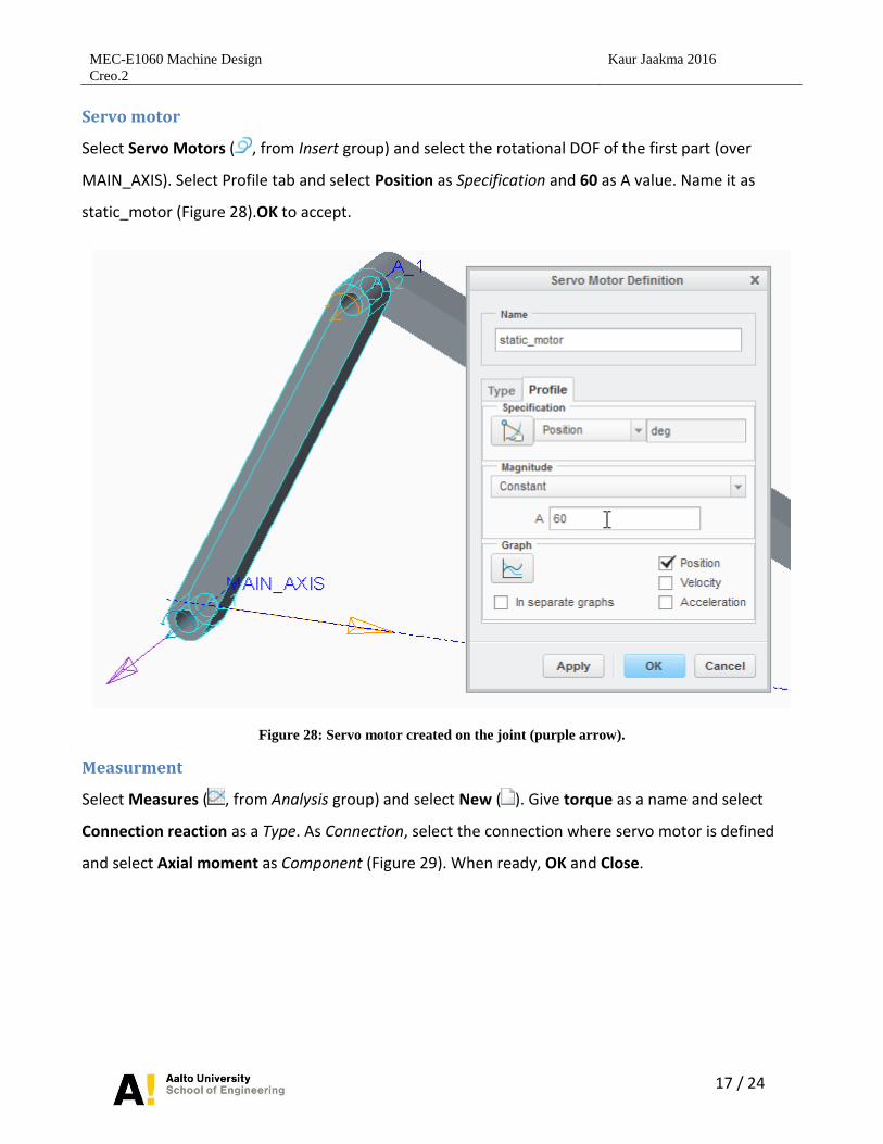
Servo motor

Select Servo Motors ( , from Insert group) and select the rotational DOF of the first part (over

MAIN_AXIS). Select Profile tab and select Position as Specification and 60 as A value. Name it as

static_motor (Figure 28).OK to accept.

Figure 28: Servo motor created on the joint (purple arrow).

Measurment

Select Measures ( , from Analysis group) and select New ( ). Give torque as a name and select

Connection reaction as a Type. As Connection, select the connection where servo motor is defined

and select Axial moment as Component (Figure 29). When ready, OK and Close.


Creo.2

18 / 24

Figure 29: Torque measurement.

Dynamic analysis

Select Mechanism Analysis ( , from Analysis group). Name it as M_torque and select Dynamic as a

Type. Change Duration to 1. Select Motors tab to check that static_motor is listed. Select External

loads tab and check option Enable gravity. Select OK to accept the simulation.

Running a simulation

In the bottom-left you can see Mechanism Tree, where all mechanism related features (motors,

connections, loads etc.) are listed. Select BODIES and expand it to see, that this model has three

bodies (one ground and two bodies). Select ANALYSES and expand it. Select M_torque, hold RMB and

select Run.

Plot result

Select Measures ( , from Analysis group). Select torque from the Measures list, M_torque from the

Result set list. Next to the torque you can see the result (~-58412). If you press Graph, you can see

the used unit system (mm2kg/sec2)


Creo.2

19 / 24

Full cycle

We want to calculate the needed torque during one cycle. Select Measures ( ) and create a New ( )

measure named deg. Type can be Position. Select the joint in the MAIN_AXIS, OK. Select deg and

previous result set (M_torque) to see, that the value is 60. Close to close the tool.

Create a new Servo Motor ( ) on the MAIN_AXIS using full_cycle as a name, Velocity as a

Specification and 36 as A value (full cycle in 10 s).

Create a new Mechanism Analysis ( ) using full_cycle as name, Dynamic as a Type and 10 as a

Duration. In Motors, unselect static_motor by selecting it and selecting Delete highlighted rows ( ).

In External loads, check Enable gravity. OK. Run the created simulation.

In Measures ( ), select Graph type as measure vs. measure and select deg as Measure for X-axis.

Then select torque as Measures and full_cycle as Result set (Figure 30). Click Graph ( ) to see the

needed torque during one cycle (Figure 30). Notice that the deg starts with 60. This is because the

defined starting angle for the mechanism. It can be changed by changing the regeneration value of

the joint to 0, if needed. Notice also, that this graph can be exported to MS Excel (File Export

Excel).


Creo.2

20 / 24

Figure 30: On left: setting for graph. On right: graphed torque.

Location of a point P

To point location of point P, use measures and make position measures to one of the points in the

middle of link part. Then graph them using one as X and other as Y-axis (Component field X and Y). The

result should be like in Figure 31. You can change the texts in the graph by selecting Format Graph.


Creo.2

21 / 24

Figure 31: Location of the point P.

Calculating Needed Volume

We can use our mechanism model to estimate how much space it needs when operating. Select

Playback ( , Analysis group). In Playback window, ensure that full_cycle is Result Set and select

Create a Motion Envelope ( , Figure 32).


Creo.2

22 / 24

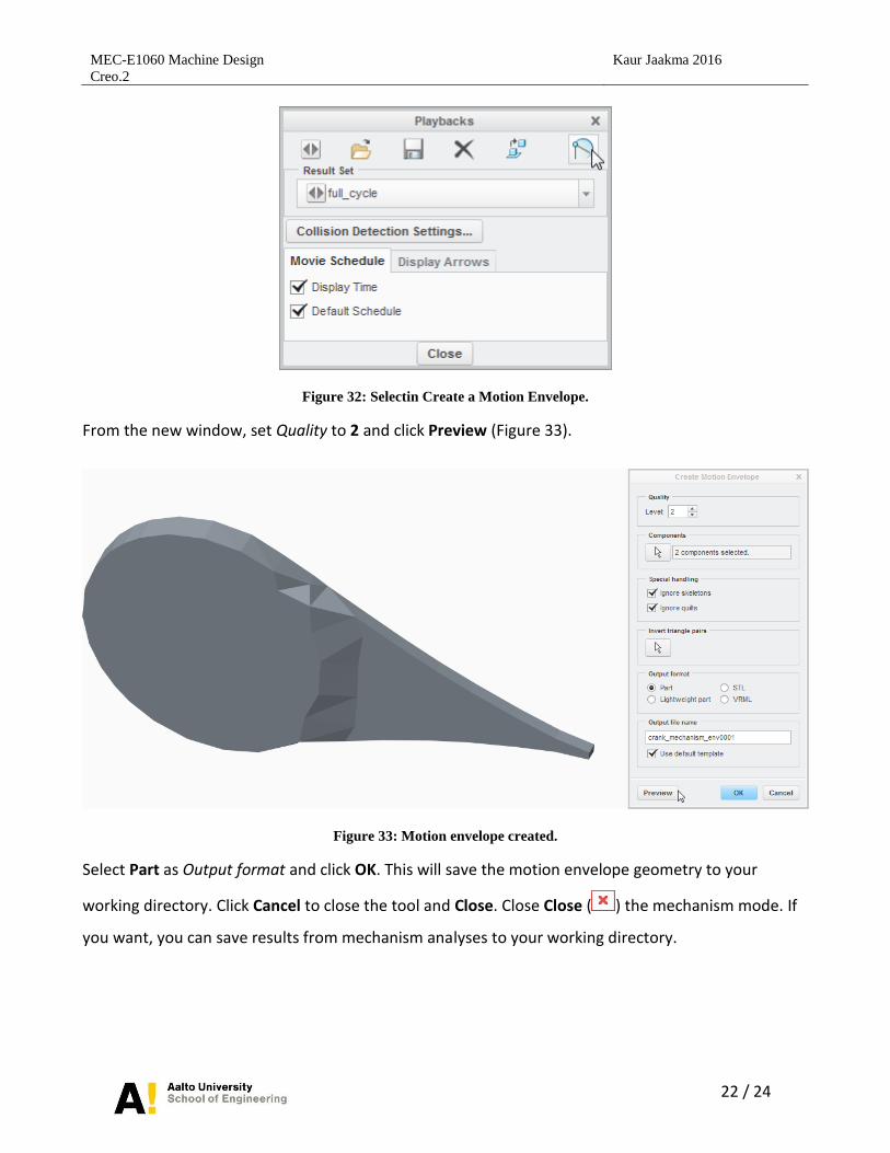
Figure 32: Selectin Create a Motion Envelope.

From the new window, set Quality to 2 and click Preview (Figure 33).

Figure 33: Motion envelope created.

Select Part as Output format and click OK. This will save the motion envelope geometry to your

working directory. Click Cancel to close the tool and Close. Close Close ( ) the mechanism mode. If

you want, you can save results from mechanism analyses to your working directory.


Creo.2

23 / 24

Click Open (Ctrl + O) and select the previously created envelope part (default name

crank_mechanism_env0001.prt). Select Analysis tab and Mass Properties ( , Model Report group).

Click Preview to calculate mass properties. If needed, you can save Mass Properties as a feature.

Bonus – Replacing Components

You can check how different dimensions affect the needed torque or the location of a point. This can

be done in the assembly mode. Select the part to be replaced (for ex. LINK_200), hold RMB and select

Replace. Click the folder icon ( ) and select a family table member (for ex. LINK_150), OK and OK.

If needed, regenerate the model (Ctrl + G). You can run the simulation again and see how this change

affect the results.

Conclusions

Now that you have a working mechanism and besides the cool animation you can perform a different

kind of measurements to better understand its performance. In the exercise you created a

measurement of the crankshaft position in degrees, other types of measurements available are:

Position — Measures the location of a point, vertex, or motion axis during the analysis.

Velocity — Measures the velocity of a point, vertex, or motion axis during the analysis.

Acceleration — Measures the acceleration of a point, vertex, or motion axis during the

analysis.

Connection Reaction — Measure the reaction forces and moments at connections.

Net Load — Measures the magnitude of a force load on a spring, damper, servo motor,

force, torque, or motion axis. You can also confirm the force load on a force motor.

Loadcell Reaction — Measures the load on a loadcell lock during a force balance analysis.

Impact — Determines whether impact occurred during an analysis at a connection limit,

slot end, or between two cams.

Impulse — Measures the change in momentum resulting from an impact event. You can

measure impulses for connections with limits, for cam-follower connections with liftoff, or

for slot-follower connections.


Creo.2

24 / 24

System — Measures several properties that describe the behavior of the entire system.

Properties that can be measured are Degrees of Freedom, Redundancies, Time, Kinetic

Energy, Linear Momentum, Angular Momentum, Total Mass, Center of Mass, and Total

Centroidal Inertia.

Body — Measures several that describe the behavior of a selected body.

Separation — Measures the separation distance, separation speed, and change in

separation speed between two selected points.

Cam — Measures the curvature, pressure angle, and slip velocity for either of the cams in

a cam-follower connection.

User Defined — Defines a measure as a mathematical expression that includes measures,

constants, arithmetical operators, Creo parameters and algebraic functions.

Belt — Measures the belt tension or slip.

3D Contact — Measures the Contact area, pressure angle, or slip velocity during contact.

As you can see the list is quite long. It is clear that for time reason we cannot propose exercises that

explore all the possible functionality. We hope that you understood how CAD models can be much

more than just a collection of geometries. Thus, in the future we expect that you will be eager to try

out the analysis feature that Creo offers.

creo.2 crank mechanism analysis - mycourses · mec-e1060 machine design kaur jaakma 2016 creo.2 3 /...

Documents