Research Division Federal Reserve Bank of St. Louis Working Paper Series

Credit Search and Credit Cycles

Feng Dong Pengfei Wang

and Yi Wen

Working Paper 2015-023A http://research.stlouisfed.org/wp/2015/2015-023.pdf

September 2015

FEDERAL RESERVE BANK OF ST. LOUIS Research Division

P.O. Box 442 St. Louis, MO 63166

______________________________________________________________________________________

The views expressed are those of the individual authors and do not necessarily reflect official positions of the Federal Reserve Bank of St. Louis, the Federal Reserve System, or the Board of Governors.

Federal Reserve Bank of St. Louis Working Papers are preliminary materials circulated to stimulate discussion and critical comment. References in publications to Federal Reserve Bank of St. Louis Working Papers (other than an acknowledgment that the writer has had access to unpublished material) should be cleared with the author or authors.

Credit Search and Credit Cycles∗

Feng Dong† Pengfei Wang‡ Yi Wen§

This Version: August 2015

First Version: March 2014

Abstract

The supply and demand of credit are not always well aligned and matched, as is reflectedin the countercyclical excess reserve-to-deposit ratio and interest spread between the lendingrate and the deposit rate. We develop a search-based theory of credit allocations to explainthe cyclical fluctuations in both bank reserves and the interest spread. We show thatsearch frictions in the credit market can not only naturally explain the countercyclical bankreserves and interest spread, but also generate endogenous business cycles driven primarilyby the cyclical utilization rate of credit resources, as long conjectured by the Austrian schoolof the business cycle. In particular, we show that credit search can lead to endogenous localincreasing returns to scale and variable capital utilization in a model with constant returnsto scale production technology and matching functions, thus providing a micro-foundationfor the indeterminacy literature of Benhabib and Farmer (1994) and Wen (1998).

Keywords: Search Frictions, Credit Utilization, Credit Rationing, Self-fulfilling Prophecy,Business Cycles.

∗We benefit from comments by the anonymous referee, Costas Azariadis, Silvio Contessi, Bill Dupor, FrancoisGeerolf (discussant), Rody Manuelli, Benjamin Pugsley, B. Ravikumar, Yi-Chan Tsai (discussant), Jose-VıctorRıos-Rull, Harald Uhlig, Randy Wright, Steve Williamson, as well as participants of 2015 ASSA meeting atBoston, the macro seminar at Federal Reserve Bank of St. Louis, the NBER conference on Multiple Equilibriaand Financial Crises at Federal Reserve Bank of San Francisco, Tsinghua Workshop in Macroeconomics 2015,and The Fourth HKUST International Workshop on Macroeconomics. The views expressed are those of theindividual authors and do not necessarily reflect official positions of the Federal Reserve Bank of St. Louis, theFederal Reserve System, or the Board of Governors. The usual disclaim applies.†Corresponding author: Antai College of Economics and Management, Shanghai Jiao Tong University, Shang-

hai, China. Tel: (+86) 21-52301590. Email: fengdong@sjtu.edu.cn‡Department of Economics, Hong Kong University of Science and Technology, Clear Water Bay, Hong Kong.

Tel: (+852) 2358 7612. Email: pfwang@ust.hk§Federal Reserve Bank of St. Louis, P.O. Box 442, St. Louis, MO 63166; and School of Economics and

Management, Tsinghua University, Beijing, China. Office: (314) 444-8559. Fax: (314) 444-8731. Email:yi.wen@stls.frb.org

1

1 Introduction

The role of financial intermediation and credit supply in driving and amplifying the business

cycle has long been analyzed in the history of economic thoughts at least since the Austrian

school. The Austrian theory of the business cycle emphasizes bank issuance of credit as the

main cause of economic fluctuations. It asserts that the banking sector’s excessive credit supply

and low interest policy (with loanable funds rate below the natural rate) drive firms’ investment

boom, and its tight credit and interest rate policy (with loanable funds rate above the natural

rate) generate economic slump.

The history of financial crisis seemed consistent with the Austrian theory. A notable feature

of financial crisis in 2007, for example, is that before the financial crisis both the bank interest

rate and the reserve-to-deposit ratio were excessively low in the economic boom period leading

to the financial crisis. On the verge of the financial crisis in late 2007 and early 2008, however,

there was excessive demand for credit on the firm side (as reflected by the interest rate hike)

and tightened credit supply on the bank side (as reflected in the significantly increased excess

reserve-to-deposit ratio). For example, according to a survey on Chief Financial Officers (CFO)

in 2008 by Campello, Graham and Harvey (2008), about 60 percent of U.S. CFOs states that

their firms are financially constrained. Among them, 86% say that they have to pass attractive

investment opportunities due to the inability to raise external financing. On the other hand,

banks were building up their cash positions at unprecedented speed. Bank excessive reserves

skyrocketed from 1.93 billion to 1043.30 billion from the second quarter of 2008 to the second

quarter of 2010, while the growth of bank loans plunged 37.17% during the same period.

Corresponding to the tight credit supply was the high interest rate on bank loans. Thus, we

observe in Figure 1 a countercyclical movement in the excess reserve-to-deposit ratio (dashed

line, re-scaled) and in Figure 2 a countercyclical movement in interest rate spread between the

loan rate and the 3-month treasury bill rate (dashed line).

However, correlation is not causation. It is not clear from the figures whether the observed

credit cycle and interest movements are endogenous outcome (symptoms) of the business cycle

or the cause of it. This paper tries to shed light on such critical issues.

Specifically, we provide a search-based financial intermediation theory to explain the ob-

served countercyclical excess reserve-to-deposit ratio and the countercyclical interest rate spread

in the data. Our main starting point is that in the real world there are always agents with sav-

ings and agents with investment projects, but the demand side of the credit market (e.g., firms)

2

and the supply side of the credit market (e.g., households and banks) need to overcome search

frictions to channel funds from savers to firms. This is especially the case in developing coun-

tries where financial markets are highly underdeveloped such that underground credit-search

market and shadow banking are pervasive. We show that such search frictions can indeed lead

to countercyclical excess reserve-to-deposit ratio and countercyclical interest rate spread. More

importantly, they can also lead to endogenous business cycles driven by self-fulfilling beliefs

on the tightness of credit conditions in the credit market. Such coordinated beliefs produce

economic fluctuations through affecting the effective utilization rate of the aggregate credit

resources. Moreover, our calibration analysis reveals that an endogenous multiplier-accelerator

propagation mechanism that is rooted in credit search is not only theoretically appealing but

also empirically plausible. The model captures many insights and predictions similar to those

described by the Australian theory.

‐2.5

‐1.5

‐0.5

0.5

1.5

2.5

3.5

4.5

GDP growth rate

Excess reserve ratio

Figure 1: GDP Growth Rate and Excess Reserve Ratio. Data Source: FederalReserve Economic Data (FRED).

Our model also sheds light on the issue of credit rationing. Credit rationing is not only

of theoretical interest, but also plays a non-trivial role in real-world firm financing. As doc-

umented in Becchetti et al (2009) based on Italian firm data, around 20.24% of firms are

subject to credit rationing in Italy. However, the literature on credit rationing is extremely

thin despite the seminal work of Stiglitz and Weiss (1983). So, in addition to shedding light on

3

the cyclical behavior of bank reserves and interest spread and credit-led business cycles, our

search-theoretical approach also provides a short cut to quantitatively study the business-cycle

property of credit rationing.

‐3

‐2

‐1

0

1

2

3

4

5

6

7

8

GDP growth rate

Interest spread

Figure 2: GDP Growth Rate and Interest Spread (Loan Rate Minus Three-MonthTreasury Bill). Data Source: FRED.

To highlight the relevance of credit-market search frictions to the business cycle, our frame-

work is by design kept extremely simple with off-the-shelf search-and-matching frictions. But

we show that the results can be very powerful despite the simplicity of the model. Specifically,

the benchmark model features three types of agents: a representative household with a contin-

uum of ex ante identical members (depositors), a representative financial intermediary (bank)

with a continuum of ex ante identical loan officers, and a continuum of firms. The banking

sector accepts deposits from the household and then lends credit to firms through search and

matching. We assume there are search frictions both between the household and the banking

sector and between the banking system and firms. We will show which search frictions are

more critical to generate self-fulfilling credit cycles.

Similar to the standard Diamond-Mortensen-Pissarides (DMP) search-and-matching model

of unemployment, our model features aggregate matching functions that determine the number

of credit relationships between depositors and financial intermediaries, and between loan officers

and firms. Such search frictions create un-utilized credit resources in equilibrium, analogous

4

to unemployed labor force in the DMP model. For example, when bank deposits are not

matched with firms, they become idle (excess reserves) in the banking system, while firms that

are unmatched with loans are considered as being denied for credit. This simple matching

framework then provides a quantitative framework to analyze and explains the coexistence of

excess reserves and credit rationing in the data. Since a booming economy encourages more

costly search in the credit market, it increases the matching probability of credit resources.

As a result, the reserve-to-deposit ratio is countercyclical over the business cycle. In addition,

since the deposit rate facing the household sector is determined mainly by time preference

(the natural rate) and the lending rate facing firms determined mainly by credit availability

and firms’ credit demand, the spread between the loan rate and the deposit rate may also be

countercyclical under aggregate shocks. Thus, our framework provides a natural interpretation

of the Australian school’s concepts of the natural rate and loanable rate of interest.

In addition, we show that such an elastic supply of credit due to variable utilization rate

of existing credit resources under search and matching can lead to local increasing returns to

scale (IRS) in the aggregate production function even though the underlying production and

matching technologies both exhibit constant returns to scale (CRS). This endogenous source

of local IRS caused by procyclical credit utilization can lead to local indeterminacy and self-

fulfilling credit cycles that feature a powerful multiplier-accelerator propagation mechanism.

In our model, an anticipated increase in credit supply from the banking sector (in the

absence of any fundamental shocks) would entice firms to increase search efforts, resulting in

more credit matches. So, more capital would be channeled from the financial sector to firms,

provided that the cost of borrowing does not increase sufficiently to discourage entry. With

more loans (capital) in hand, firms can increase production by hiring more labor, so households’

labor supply would also increase, leading to higher aggregate income and household savings.

If the increase in household savings is large enough, it would then increase bank deposits

and raise bank’s credit supply without too much upward pressure on the loanable funds rate,

ratifying firms’ initial optimistic expectations about credit conditions. But the process does

not stop here. Because of higher deposit, competition among banks will reduce the loan rate,

which induces more firm to enter the credit market to search for loans. More firm-entry in turn

would further increase the matching probability, raising the effective capital stock used in firms’

production even more. Consequently, the economy can enter a persistent boom period (after

an initial shock) that features all the symptoms of a credit cycle described by the Austrian

school; namely, a seemingly easy credit policy is associated with a higher lending volume,

5

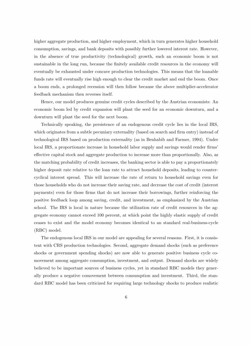
higher aggregate production, and higher employment, which in turn generates higher household

consumption, savings, and bank deposits with possibly further lowered interest rate. However,

in the absence of true productivity (technological) growth, such an economic boom is not

sustainable in the long run, because the finitely available credit resources in the economy will

eventually be exhausted under concave production technologies. This means that the loanable

funds rate will eventually rise high enough to clear the credit market and end the boom. Once

a boom ends, a prolonged recession will then follow because the above multiplier-accelerator

feedback mechanism then reverses itself.

Hence, our model produces genuine credit cycles described by the Austrian economists: An

economic boom led by credit expansion will plant the seed for an economic downturn, and a

downturn will plant the seed for the next boom.

Technically speaking, the persistence of an endogenous credit cycle lies in the local IRS,

which originates from a subtle pecuniary externality (based on search and firm entry) instead of

technological IRS based on production externality (as in Benhabib and Farmer, 1994). Under

local IRS, a proportionate increase in household labor supply and savings would render firms’

effective capital stock and aggregate production to increase more than proportionally. Also, as

the matching probability of credit increases, the banking sector is able to pay a proportionately

higher deposit rate relative to the loan rate to attract household deposits, leading to counter-

cyclical interest spread. This will increase the rate of return to household savings even for

those households who do not increase their saving rate, and decrease the cost of credit (interest

payments) even for those firms that do not increase their borrowings, further reinforcing the

positive feedback loop among saving, credit, and investment, as emphasized by the Austrian

school. The IRS is local in nature because the utilization rate of credit resources in the ag-

gregate economy cannot exceed 100 percent, at which point the highly elastic supply of credit

ceases to exist and the model economy becomes identical to an standard real-business-cycle

(RBC) model.

The endogenous local IRS in our model are appealing for several reasons. First, it is consis-

tent with CRS production technologies. Second, aggregate demand shocks (such as preference

shocks or government spending shocks) are now able to generate positive business cycle co-

movement among aggregate consumption, investment, and output. Demand shocks are widely

believed to be important sources of business cycles, yet in standard RBC models they gener-

ally produce a negative comovement between consumption and investment. Third, the stan-

dard RBC model has been criticized for requiring large technology shocks to produce realistic

6

business cycles (see King and Rebelo (1999) for a survey of the literature). Thanks to the

endogenous IRS in our model, small fundamental shocks (either demand or supply shocks, in-

cluding news shocks) can generate large business cycle fluctuations with positive comovements,

without assuming various types of adjustments costs and special utility functions. Fourth, our

model can generate indeterminacy and self-fulfilling business cycles with hump-shaped output

responses without productive externalities as in the model of Benhabib and Farmer (1994) and

the variable capacity utilization model of Wen (1998).

Our paper is related to several strands of literature. First, the search friction is in line

with approaches proposed by Den Haan, Ramey and Waston (2003), Wasmer and Weil (2004),

and Petrosky-Nadeau and Wasmer (2013). These researchers have explored the implication

of credit search on macroeconomy, but does not study the possibility of indeterminacy. For

simplicity and tractability, they have assumed linear utility. In contrast, we incorporate the

credit search friction into an otherwise standard RBC model. This allows us to study a richer

set of economic variables of interest. Our paper is also inspired by search frictions in goods

market such as Bai et al (2012), and by search-theoretic models of asset trading such as Duffie,

Garleanu and Pederson (2005) and Lagos and Rocheteau (2009). Recently Cui and Radde

(2014) incorporate such line of research into a dynamic general equilibrium model and show it

can explain the interesting flight-to-liquidity phenomena observed in great recession.

Our model also provides a micro foundation for the Benhabib-Farmer (1994) model with

IRS and the Wen (1998) model with variable capital utilization rate under IRS. We show

that search frictions in the credit market can generate an economic structure isomorphic to

the Benhabib-Farmer-Wen model with both increasing returns and elastic capacity utilization,

yet without assuming IRS in the production technology of firms. Our paper is also closely

related to several recent works on self-fulfilling business cycle due to credit market frictions,

such as Gertler and Kiyotaki (2013), Miao and Wang (2012), Benhabib, Miao and Wang (2014),

Azariadis, Kaas and Wen (2014), Pintus and Wen (2013), Liu and Wang (2104), and Benhabib,

Dong and Wang (2014).

Finally, our model is in the same spirit of Acemoglu (1996), who shows that search friction

in labor market generate increasing returns to human capital accumulation in a two-period

model. In his model, the workers have to make human capital investments before they enter

the labor market. An increased in the average human capital investment induce more physical

investments from firms. So even some of workers who have not increased their humane capital

will earn a higher return on their human capital if matched with firms. In other words, search

7

friction produce a positive pecuniary externality similar to the mechanism in our model. How-

ever, unlike Acemoglu (1996), we focus on search in credit market and explore its implication on

indeterminacy and self-fulfilling expectation driven business cycles in an infinite-period model.

The rest of the paper is organized as follows. Section 2 and Section 3 lays out the baseline

model, and examines its key properties respectively. Section 4 studies the model’s business

cycle implications under calibrated parameter values. Section 5 extends the baseline model,

and Section 6 concludes the paper. The omitted proofs in the context are put in the appendix.

2 Model

2.1 Environment

Time is continuous. The economy is populated by three types of agents: a representative

household composed of a continuum of depositors, a representative bank (financial intermedi-

ary) composed of a continuum of clerks or loan officers, and a continuum of firms. We assume

perfect competition in all sectors. The household owns capital and firms, makes decision on

labor supply and consumption, and deposits savings into the banking system, which channels

capital (in the form of loans) to firms. To break the conventionally assumed accounting identity

between aggregate household saving and firm investment (which was criticized by the Austrian

school and Keynes), we assume search frictions among the three types of agents so that in equi-

librium aggregate household saving does not automatically equal firm investment, but instead

imposes an upper limit on firm investment for any given interest rate.

The time line of events in an interval of t and t+ dt is as follows. First, loan officers search

for depositors to collect bank reserves; or alternatively, depositors search for loan officers to

deposit their savings (carried over from the last period) into the banking system. So there

is a search-and-match friction between depositors and the banking system. Without loss of

generality, we assume that the household pays for the search costs. After collecting deposits,

the loan officers and firms engage in random search and match.1 Again we assume that firms

pay for the search costs. In order to enter the credit market, however, a firm needs to pay

a fixed cost. If a firm gets matched successfully and obtains a loan, trading surplus is split

between the firm and the bank and the credit relationship is then dissolved by the end of the

period.2 After obtaining a loan (capital), firms can start producing goods by hiring labor in

1See Section 5.3 for an alternative setup with competitive search. All the qualitative results derived in thispaper are preserved under competitive search.

2We address the issue of long-term credit relationships in a companion paper, but the basic results hold.

8

the spot market. The number of active firms engaging in production is then determined by the

free entry condition: the expected surplus from a successful match equals the fixed search cost

of entering the credit market. Finally, the household pools wage and profit incomes from the

bank and firms and then makes decision on consumption and capital accumulation (next-period

savings). The whole process is repeated analogously in the next time interval between t + dt

and t+ 2dt.

To facilitate the analysis, we assume that all depositors from the household are ex ante

identical and assigned with the same amount of credit resources to be randomly matched with

a continuum of ex ante identical loan officers. Any unmatched savings are kept as inventories

and carried over to the next period by the household. Analogously, after collecting deposits

from the household, all loan officers are assigned with the same amount of credit resources

available and go out to be randomly matched with firms. Any unmatched loans are counted as

excess reserves, and transferred lump sum back to the households in the end of each period.3

Specifically, denote S as the total savings of the household. Due to search frictions, only

S < S units of savings are successfully matched and deposited into the banking system. After

that, each loan officer is assigned with an equal fraction of the S units of deposits and goes out

searching for potential borrows (firms).

We show that such a simple setup leads to a simple dynamic system that can generate

(i) countercyclical excess reserve-to-deposit ratio, (ii) countercyclical interest rate spread be-

tween the loan rate and the deposit rate, and (iii) self-fulfilling business cycles with strong

amplification and propagation mechanisms.

2.2 Deposit Search

We first consider search frictions between the household and the banking system. The matching

function between household members and bank clerks is MH (xtHt, Bt) = γH (xtHt)εH B1−εH

t ,

where xt is the search effort chosen by household depositors. There is a unit measure of

household depositors and bank clerks, i.e., Ht = Bt = 1.4 Thus, the probability of match is

given by

et =MH (xtHt, Bt)

Ht= γHx

εHt . (1)

3In a follow-up project, we study the case with required reserves and interbank lending.4Our results would be strengthened if we allow Ht and Bt to vary by costly entry as an additional margin of

adjustment.

9

Denoting dt as the time interval, the budget constraint of the household can be written as [the

original budget constraint is ]

Ctdt+ St+dt =[et

(1 +Rdt dt

)− φHxtdt

]St + (1− et)St +WtNtdt+ Πtdt (2)

subject to equation (1), where Ct denotes consumption, St total savings, et the fraction of

aggregate savings successfully deposited into the banking system, Rdt the deposit rate promised

by the bank, xt the search effort devoted by the household, WtNt the wage income and Πt the

profit income from banks and firms, which are to be specified later. Note the first term on

the right-hand side (RHS) pertains to the cross rate of return to deposits per unit of savings,

et(1 +Rdt

), after subtracting the search cost per unit of savings in hand, φHxt. That is, we

assume that the search cost for each depositor is proportional to her effort xt and the stock of

savings in hand.5 The second term on the RHS, (1− et)St, is the total idle (unmatched) credit

resources, which is also the unmatched ”inventory” stock of savings kept by the household.

The first-order-condition (FOC) of the effort choice is given by xt =[(

γHεHφH

)Rdt

] 11−εH . In

turn, the aggregate utilization rate of household savings is et = γH

[(γHεHφH

)Rdt

] εH1−εH . Because

of the search costs, we can derive a pseudo ”depreciation” function of the stock of savings as

follows. Denoting δ0 ≡ φH(1+κ)

γ1+κH

and κ ≡ 1εH− 1, we can define

δ (et) ≡ φH(etγH

) 1εH

≡ δ0

(e1+κt

1 + κ

), (3)

as a ”depreciation” function of the saving stock, which is convex in the utilization rate (et) of

savings, analogous to Wen’s (1998) model. With this notation and taking the limit dt→ 0, the

household budget constraint in equation (2) becomes

Ct + St = WtNt +[etR

dt − δ (et)

]St + Πt. (4)

Then we can formulate the constrained optimization problem of the representative household

in a continuous-time model as

max

∫ +∞

0e−ρt

[log (Ct)− ψ

N1+ξt

1 + ξ

](5)

subject to equation (4), where ρ > 0 is the discount factor, ψ > 0 controls the utility weight on

labor supply, and ξ > 0 is the inverse Frisch elasticity of labor supply. The first order conditions

5We choose this proportional cost function so as to compare with the fixed search cost on the firm side (tobe specified below). This way we can show which form of the search costs leads to local IRS in our model.

10

of the household with respect to labor (Nt), consumption (Ct), saving (St), and search effort

(et) are given by

CtCt

= etRdt − δ (et)− ρ, (6)

Wt

Ct= ψN ξ

t , (7)

Rdt = δ′ (et) = δ0eκt (8)

2.3 Loan Search

The loan market consists of a large number of credit lenders (loan officers) and borrowers

(firms). More specifically, there are Bt number of loan officers and Vt number of firms. Note

that the total deposits in the banking system are given by St = etSt, which are divided equally

among the loan officers (with measure Bt = 1). Each firm needs to pay a fixed cost φt to enter

the credit market to search for lenders. If a firm is matched with a loan officer, it can produce

yt = AtSαt n

1−αt units of output, where nt is the labor input of the matched firm. The search

friction is captured by a matching technology M (B, V ), where V denotes the measure of firms

entering the credit market after paying the fixed entry cost φ. To make the results sharp and

tractable, we also assume a Cobb-Douglas matching technology, M (B, V ) = γB1−εV ε, with

ε ∈ (0, 1). Denoting θt ≡ BtVt

as a measure of the credit market tightness, the probability that

a firm can match with a credit supplier is

qt ≡M (Bt, Vt)

Vt= M (θt, 1) = γθ1−ε

t , (9)

and the probability that a loan officer can match with a firm is given by

ut ≡M (Bt, Vt)

Bt= M

(1,

1

θt

)= γθ−εt . (10)

Note that ut is also the utilization rate of total bank deposits. That is, the aggregate amount

of capital lent out successfully to firms is utSt. Notice that

Vtqt = M (Bt, Vt) = Btut. (11)

11

Given real wage wt, if a firm is successfully matched, its operating profit (the matching surplus)

is given by Πt = maxnt≥0

AtS

αt n

1−αt −Wtnt

. Hence, based on the FOC of nt, we obtain

nt =

[At

(1− αWt

)] 1α

St, (12)

Πt = αAt

[At

(1− αWt

)] 1−αα

St ≡ πtSt. (13)

Notice from Equation (13) that a successfully matched firm’s operating profit is proportional

to the total bank deposits St (as we assume that total bank deposits are divided equally among

the loan officers and the measure of loan officers is Bt = 1).

For each successful match, the operating profit (surplus) is split between the firm and the

loan officer by Nash bargaining, with the firm obtaining η ∈ [0, 1] fraction of the surplus.

Denote Rlt as the competitive interest rate on loans, then it must be true that the lending

interest rate equals the expected rate of return to the loan:

Rlt = (1− η)πt. (14)

A firm’s ex ante expected surplus before conducting credit search is qtηπtSt. Hence, the

free entry (zero profit) condition for the firms is given by

φt = qtηπtSt. (15)

Then equations (9) and (15) together imply

qt = γθ1−εt =

φt

ηπtSt. (16)

This equation states that the probability of match for a firm, qt, decreases with the volume

of match surplus. The intuition is as follows. A higher match surplus will induce more firms

to enter, hence reduces the probability of each firm’s match with the given number of credit

suppliers.

The banking sector is perfectly competitive and thus makes zero profit. The bank needs to

pay the depositors the deposit rate Rdt , and earn the rate of return Rlt (the lending rate) with

probability ut. Therefore the zero profit condition for the banking sector is given by

Rdt = utRlt. (17)

This equation captures the interest rate spread. Finally the aggregate net profit income dis-

tributed to the household is given by Πt =(−Rdt + utR

lt

)St + (−φ+ qtηπt)Vt = 0. Note that

12

although for simplicity we have assumed that the measures of depositors and loan officers are

all unity (Ht = Bt = 1), the number of firms Vt in the credit market is however a variable.

3 General Equilibrium Analysis

A general equilibrium is defined as a collection of prices Wt, Rdt , R

lt and quantities Ct, St, Nt,

Vt, πt, nt, St,Kt, et, ut, qt such that (i) given prices and aggregate profit income Πt, the alloca-

tion Ct, St, Nt solves household’s utility maximization problem defined in (5); (ii) the surplus

πt and labor input nt for a successfully matched firm are defined by (13) and (12); (iii) given

the probability ut of being matched with a bank loan officer, the equilibrium number of firms

Vt is determined by the free entry condition (15); (iv) given the bank’s probability of matching

with a firm (ut), the bank earns zero expected profit as characterized by (17); (v) in the credit

markets, the probability qt and ut are determined by (9) and (10), (vi) both labor markets and

goods markets satisfy the standard market-clearing conditions.

3.1 Aggregate Production Function

Proposition 1 In general equilibrium, the aggregate production function can be represented as

Yt = At (etutSt)αN1−α

t . (18)

Proof: See Appendix.

To complete the characterization of the aggregate system, we can show that the aggregate

surplus from successful matches between loan officers and firms is then given by

πt ≡ αAt[At

(1− αWt

)] 1−αα

= α

(YtKt

), (19)

which is equals to the marginal product of aggregate capital. The deposit rate is then given

by Rdt = utRlt = α (1− η)

(YtSt

). The last equality is obtained by combining Kt = VtqtSt and

Equation (11). Since B = 1, and ut = γθ−εt , the aggregate entry costs V φ satisfy

V φ =

(B

θ

)φ = ∆ (u) ≡ ∆0

u1+λ

1 + λ, (20)

where ∆ (u) is convex with u with ∆0 ≡ φ(1+λ)γ1+λ

and λ ≡ 1ε − 1 > 0.

13

3.2 Local IRS and Local Indeterminacy

Combining equations (8), (17), (14) and (19) yields

et = e

(YtSt

)εH, (21)

where e ≡(α(1−η)(1−σ)

δ0

) 11+κ

and κ ≡ 1εH−1. Additionally, the free entry condition (15) implies

V φ = V qηπS = αηY. (22)

Combining equation (20) and (22) then yields

ut = uY εt , (23)

where u ≡[αη(1+λ)

∆0

] 11+λ

, ∆0 ≡ φ(1+λ)γ1+λ

, and λ ≡ 1ε − 1.

Proposition 2 The aggregate production function in equation (18) exhibits local IRS (local

increasing returns to scale) in household capital (St) and labor supply (Nt), because it can be

rewritten as

Yt = Y Aτt Sαst Nαn

t , (24)

where Y ≡[(1− η)εH

(ηε

)ε ( αδ0

)εH ( αη∆0

)ε] α1−α(ε+εH) , τ ≡ 1

1−α(ε+εH) > 1, αs ≡ α (1− εH) τ > α,

and αn ≡ (1− α) τ > 1− α with the degree of aggregate returns to scale given by

αs + αn > 1. (25)

Proof: See Appendix.

As shown in condition (25), we obtain aggregate IRS in household capital St and labor

supply Nt despite the lack of Benhabib-Farmer type production externalities. This is due to

the endogenously time varying utilization rate of aggregate household savings and aggregate

bank deposits, as suggested by Equations (21) and (23). However, the IRS are local because

the capital utilization rates, et and ut, are both bounded by the interval [0, 1]. Meanwhile,

since τ > 1, we also obtain the amplification effect on productivity shock.

It is obvious that our model based on credit search appears isomorphic to the IRS models

of Benhabib and Farmer (1994) and Wen (1998). Hence, our model may also give rise to local

indeterminacy and self-fulfilling business cycles with strong propagation mechanisms as in their

models. To understand the intuition, consider a proportional increase in aggregate labor and

14

capital supply from the household. In a standard neoclassical model without credit search,

such a proportional increase in labor and capital supply would only increase aggregate output

one-for-one. However, in our model the increase of household savings leads to a higher credit

supply in the banking system, which in turn would reduce the cost of borrowing and hence

induce more firms to enter the credit market, which in turn increases the match probability

of credit resources, raising the effective capital stock used in the production sector more than

one-for-one, thus resulting in more than proportionate increase in aggregate output.

In addition to generating the IRS effects, the initial increase in household labor and capital

supply can also become self-fulfilling. As the effective capital used in production increases,

the returns to labor supply also increase for every household, reinforcing the initial increase in

household labor supply. In addition, as the matching probability of bank increases, bank is able

to pay a higher deposit rate. This will increase the returns to saving even for the households

who do not increase their savings. Hence, the social increasing returns to scale originate from

a subtle pecuniary externality that reinforces and multiplies itself in a positive feedback loop

just like in the model of technological production externalities.

Proposition 3 The model is locally indeterminate if and only if either of the following condi-

tions hold:

1. α ∈(0, 1

2

), ξ ∈ [0, α

1−2α), ε, εH ∈ [0, 1] and ε+ εH > ε ≡(

1α

) (α+ξ1+ξ

).

2. α ∈ [12 , 1), εH ∈ [0, 1] and 0 ≤ ε < 1

α − 1.

Proof: See Appendix.

Some comments are in order. First, when α ∈(0, 1

2

), ξ ∈ [0, α

1−2α), which is line with

our calibration in Table 1, then we know that(

1α

) (α+ξ1+ξ

)∈ [1, 2) and thus η∗ = ε

ε+εH< ε.

The indeterminacy region for this scenario is illustrated in Figure 3. Second, note that the

indeterminacy conditions have nothing to do with the bargaining power parameter η. Therefore,

indeterminacy always exists under conditions specified in the above proposition regardless we

adopt random search with Nash bargaining or competitive search (as shown in the Appendix).

Third, our model provides a micro foundation to the models of Benhabib and Farmer (1994)

and Wen (1998), which reply on exogenously assumed IRS in firms’ production technologies.

We show, instead, that such IRS technologies can be derived from credit search under CRS

technologies and matching functions.

15

𝜶 + 𝝃

𝜶(𝟏 + 𝝃)

𝜶 + 𝝃

𝜶(𝟏 + 𝝃)

𝑰𝒏𝒅𝒆𝒕𝒆𝒓𝒎𝒊𝒏𝒂𝒄𝒚

𝟏 𝑶

𝜺𝑯

𝜺

𝟏

Figure 3: Indeterminacy Region (When α ∈(0, 1

2

), ξ ∈ [0, α

1−2α))

4 Quantitative Exercises

4.1 Calibration

The time discounting factor is ρ = 1β − 1 = 0.01, where β = 0.99 denotes the discount factor

in discrete time models. We set the capital’s share α = 0.33, the coefficient of labor disutility

ψ = 1.75 and the inverse Frisch elasticity of labor supply ξ = 0.2. All of them are standard in

the existing literature.

Now we have to calibrate the values of (εH , φ, η, γ, ε), which are specific to our model.

First, as shown in the previous section, Rd = ρ(1+κ)κ where κ ≡ 1

εH− 1. We can obtain the

average deposit rate Rd from Federal Reserve Economic Data (FRED), which implies κ = 0.23,

and thus εH = 11+κ = 0.82. Second, we have proved that S

Y = α(1−η)Rd

in the steady state.

Consequently, the bargaining power of firms, η, is obtained as η = 1−(Rd

α

) (SY

)= 0.187.

It remains to pin down (φ, γ, ε). First, we interpret φ as the cost of intermediation to

financing firm investment, which pertains to the size of the financial sector. Philippon (2012)

argues that the share of financial industry is around 8% of GDP. Therefore, we set φY = 8%.

Note that φY is related to (φ, γ, ε). Second, we set u = 67% according to data on the utilization

16

rate of capital in the manufacturing sector, and we also know that u is related to (φ, γ, ε).

Finally, Becchetti et al (2009) documents that the proportion of Italian firms subject to credit

rationing is around 20%. We assume the rate of credit rationing is 15% in the U.S. Then the

proportion of matched firms is q = γθ1−ε = 85%, where θ is also related to (φ, γ, ε). Therefore

the three moments,(φY , u, q

)jointly implies that φ = 0.086, γ = 0.797 and ε = 0.729. Our

calibration exercise shows that εH +ε >(

1α

) (α+ξ1+ξ

). Consequently indeterminacy due to credit

search is empirically plausible in our model. The calibration is summarized in Table 1.

Table 1. Calibration

Parameter Value Description

ρ 0.01 Discount factorA 1 Normalized aggregate productivityα 0.33 Capital income shareψ 1.75 Coefficient of labor disutilityξ 0.2 Inverse Frisch elasticity of labor supplyεH 0.82 Matching elasticity in 1st Stage Searchη 0.187 Firm’s bargaining powerφ 0.086 Vacancy cost to search for credit.γ 0.797 Matching efficiency in 2nd stage searchε 0.729 Matching elasticity in 2nd stage search

4.2 Impulse Responses

This subsection investigates the dynamic effect of TFP shocks and matching efficiency shocks

(γt) on aggregate output, the interest spread, the utilization rate of credit (the opposite of

the reserve-to-deposit ratio), and credit rationing. All shocks have AR(1) persistence with the

persistence coefficient of 0.9. We discretize our model to facilitate the analysis.

Figure 4 shows the model’s impulse responses to a 1% TFP shock. Several striking features

of the model are worth noticing. First, the responses of aggregate output are hump-shaped.

Second, there exists a dynamic multiplier-acclerator effect or endogenous propagation mecha-

nism such that not only the maximum response of output is postponed for several periods after

the impact of the shock and it far exceeds 1%, but the impact of the shock is also long lasting

with boom-bust cycles or an over-shooting and mean-reverting cyclical pattern. Third, both

the reserve-to-deposit ratio (the negative of the top-right panel) and interest spread (lower-left

panel) are countercyclical, consistent with the data.

Similarly, Figure 5 shows that a 1% credit matching efficiency shock can also generate the

boom-bust cycles in aggregate output as well as countercyclical reserve-to-deposit ratio and

17

5 10 15 20 25 30 35 40 45 50 55 60

-10

-5

0

5

10

Output(%)

5 10 15 20 25 30 35 40 45 50 55 60-5

0

5

Utilization(%)

5 10 15 20 25 30 35 40 45 50 55 60

-0.5

0

0.5

Spread(%)

Figure 4: Impulse Responses to TFP Shock (A)

interest spread. Additionally, Figure 6 documents the impulse response driven by an i.i.d.

sunspot shock to labor supply.6 Despite the lack of any persistence in the sunspot shock, the

responses of the economy to such an shock still exhibit high persistence with a boom-bust style

similar to that under persistent fundamental shocks (except the lack of the initial hump).

To understand the intuition, consider an anticipated increase in credit supply from the

banking sector. This optimistic expectation by firms would entice them to increase search

efforts and compete for loans in the credit market, resulting in more banking capital being

channeled into firms. Firms can thus increase production by hiring more labor, so households’

labor supply also increases, leading to higher aggregate income and household savings. More

household savings would then increase bank deposits and raise bank’s credit supply without

upward pressure on the loanable funds rate, fulfilling firms’ initial optimistic expectations about

cheap credit conditions.

However, an economic boom, once kick-started by a shock (whatever they are), is going

to go through a ”natural course” of continuous expansion before returning back to the steady

6Alternatively, we can implement the impulse response by sunspot shock to consumption demand, whichdelivers a qualitatively similar result. See Wen (1998) for more details on how to introduce sunspot shocks inindeterminate DSGE models.

18

state. The positive feedback loop from firms’ production to household income under local IRS

means that any increase in firm production would lead to a more than proportionate increase

in household savings and bank deposits in the initial periods of the boom, which induces more

bank lending and firm-entry in the credit market to search for loans, especially if the shock is

expected to persist despite with a damping magnitude.

5 10 15 20 25 30 35 40 45 50 55 60-5

0

5

Output(%)

5 10 15 20 25 30 35 40 45 50 55 60

-2

0

2

Utilization(%)

5 10 15 20 25 30 35 40 45 50 55 60

-0.2

-0.1

0

0.1

0.2

Spread(%)

Figure 5: Impulse Responses to Credit Shock, i.e., Matching Efficiency Shock (γ)

However, in the absence of permanent productivity (technological) growth, such an eco-

nomic boom is not sustainable in the long run, because the IRS is only a local property. Once

the utilization rate of aggregate credit resources becomes high enough before reaching 100%,

the cost of borrowing will ultimately dominate the rate of return to capital (the marginal prod-

uct of capital) under diminishing marginal product of capital in the production technology.

Hence, the available credit resources in the economy will eventually be exhausted. This implies

that after a peak in the boom period, in each subsequent round of the positive feedback mech-

anism between the banking sector and firms, the additional volume of loans unleashed from

the banking sector becomes less and less, ultimately leading to rapid increases in the loanable

funds rate. This would eventually chock of credit demand on the firm side because the rising

costs of credit borrowing cannot be compensated by the falling (diminishing) marginal product

19

of capital as the boom continues. Hence, sooner or later the economy will stop growing and

enter a contraction phase.

Once the contraction sets in, the above feedback (multiplier-accelerator) mechanism reverses

itself and leads to a persistent period of recession. The recession features a shrinking credit

market with both very little credit-search effort by firms and rapidly accumulating excess

reserves in the banking sector. However, a prolonged recession cannot be an equilibrium state

either, because the economy will eventually reach a point at which the marginal product of

capital becomes so high (due to lack of effective investment) and the loanable funds rate becomes

so low (due to lack of credit demand and an increasing excess reserve-to-deposit ratio), which

will then cause another round of over-shooting (except with more dampened magnitude) as the

economy converges back to the steady state from below.

Hence, our model produces genuine credit cycles broadly consistent with what the Austrian

theory describes. Namely, an economic boom featuring a low interest spread (loanable funds

rate below the natural rate) plants the seed for an economic recession, and a recession featuring

a high interest spread (loanable funds rate above the natural rate) plants the seed for the next

boom. The turning point of the business cycle appears to be determined by the relative

magnitude of the loanable funds rate and the natural rate.

5 10 15 20 25 30 35 40 45 50 55 60-2

0

2

4

Output(%)

5 10 15 20 25 30 35 40 45 50 55 60-1

0

1

2

Utilization(%)

5 10 15 20 25 30 35 40 45 50 55 60-0.2

-0.1

0

0.1

0.2

Spread(%)

Figure 6: Impulse Responses to Sunspot Shock

20

5 Discussions

5.1 Eliminating Household Search Friction

Notice that if εH = 0, namely, if there is no household search, then et = 1 and we obtain

Yt = A (utSt)αN1−α

t , where ut = γ(αηYtφ

)ε. Hence, the aggregate production function becomes

Yt =[γ(αηφ

)ε]αsAτt S

αst Nαn

t , where αs ≡ ατ , αn ≡ (1− α) τ , and τ ≡ 11−αε . This production

technology still exhibits local IRS because αs+αn = 11−αε > 1. So the model appears isomorphic

to the Benhabib-Farmer model. However, because the IRS are local in our model whereas

they are global in the Benhabib-Farmer model, indeterminacy is not possible in our model

with εH = 0 although we do have endogenous IRS, except locally. On the other hand, if

we only allow household search but no firm search, i.e., ε = 0 and εH > 0, then the model

becomes isomorphic to Wen’s (1998) model without IRS, which is the Greenwood et al (1988)

model. Hence, adding household search into the model is necessary to generate indeterminacy,

analogous to Wen’s (1998) finding that variable capacity utilization can significantly reduce

the required degree of IRS in the Benhabib-Farmer model for indeterminacy. The well-known

problem of the Benhabib-Farmer model is that it requires extremely large IRS to generate

indeterminacy, which is empirically implausible. Wen’s (1998) model can reduce the required

IRS for indeterminacy down to empirically plausible range. Hence, our model provides a micro

foundation for the indeterminacy literature pioneered by Benhabib and Farmer (1994) and Wen

(1998) because we show that the Romer type IRS and Greenwood et al type capital utilization

are not needed to generate essentially identical boom-bust business cycles obtained in Wen

(1998).

5.2 Hosios Condition and Welfare

Since we have used random search to characterize frictions in the credit market, it is natural for

us to check whether the Hosios (1990) condition holds in our environment. Given (At, St, Nt),

i.e., if we control the technology and the supply of capital and labor, then the Hosios condition

is obtained by solving the following constrained optimization problem of the social planner:

maxet,utYt (et, ut)− δ (et)St −∆ (ut) , (26)

where Y (e, u), δ (e) and ∆ (u) are defined in equation (18), (3) and (20) respectively. Then we

reach a modified Hosios condition as below.

21

Proposition 4 (Modified Hosios Condition) Given (At, St, Nt), The ratio of output in the

decentralized economy to that in the social planner economy is given by

Y DE

Y SP=[(1− η)εH

(ηε

)ε] α1−α(ε+εH) , (27)

and thus

η∗ = arg maxη∈[0,1]

(Y DE

Y SP

)=

ε

ε+ εH. (28)

Several remarks are in order. First, when search frictions exist only between banks and

firms, i.e., εH = 0, then Y DE = Y SP if and only if η = ε, which shares a flavor of the classic

Hosios condition. However, in contrast to the classic Hosios condition, η = ε does not maximize

Y DE . Second and more interestingly, we contribute to the literature by detecting a modified

Hosios condition in the presence of dual search frictions, i.e., εH > 0 and ε > 0. Intuitively,

the increase of firm’s bargaining power η delivers two competing effects. On the one hand,

the increase of η intensifies firm’s search for credit by inducing more firm entry. This in turn

increases u, the utilization rate of credit in the second link of the search-and-matching chain,

and thus drives up output. On the other hand, a higher η dampens the profit share of the bank

by lowering the loan rate, which translates into a lower deposit rate, and therefore discourages

the search effort of household for the decision of deposit making. Therefore Equation (28)

strikes a balance between these two competing effects. In particular, η∗ increases with ε (the

matching elasticity of firms searching for credit) and decreases with εH (the matching elasticity

of household searching for financial intermediation). Notice that η∗ = ε if and only if ε+εH = 1.

As shown in the next subsection, ε+ εH > 1 when indeterminacy emerges, and thus η∗ < ε in

that scenario.

Finally, in deriving the Hosios conditions, we have so far followed the literature by holding

the supply of labor and capital as fixed. This restriction is fine when it comes to the standard

setup of macro labor economics a la DMP, which typically assumes inelastic labor supply and

does not take into account capital accumulation, in addition to the assumption of risk neutral

firms and workers. However, our paper has to address both of these issues since the household

in our model is allowed to make decision on labor supply as well as capital accumulation.

Moreover, the household is risk averse when it comes to consumption. As a result, neither

the classic nor the modified Hosios condition can guarantee a constrained optimum in welfare.

Instead, we have to take into account the effect of η on both consumption and leisure decisions

of the household over the lifetime horizon. Note that the household welfare in the steady state

22

0 0.1 0.2 0.3 0.4 0.5 0.6 0.7 0.8 0.9 1-200

-180

-160

-140

-120

-100

: Bargaining Power of Firm

Ω:Welfare

Welfare

Classic Hosios Condition: =

Modified Hosios Condition: = (+ )

Calibrated

Optimal

Figure 7: Hosios Conditions and Welfare: A Numerical Example (See Table 1 forParameterization)

is

Ω =1

ρ

log

[(C

Y

)Y

]− ψN

1+ξ

1 + ξ

,

where CY =

(1− α

1+κ

)−(

κ1+κ

)αη, N =

(1−αψ

1C/Y

) 11+ξ

, and Y =[A(γ(αηφ

)ε)α (SY

)αN1−α

] 11−α(1+ε)

denote respectively the steady state of the ratio of consumption to output, labor supply and out-

put, all of which are obtained from the simplified dynamical system in the proof of Proposition

3. Figure 7 indicates that in the presence of risk aversion, endogenous capital accumulation,

and elastic labor supply, neither the classic Hosios condition (i.e., η = ε) nor the modified

Hosios condition (i.e., η = εε+εH

) maximizes the household’s welfare in steady state.

5.3 Competitive Search

For simplicity, we have adopted random search in the baseline model. Alternatively, we can

use competitive search a la Moen (1997). More specifically, each loan officer can post her own

terms of trade, Rl, in sub-market θ such that

maxu (θ)Rl (θ) S

(29)

23

subject to

q (θ)[π −Rl (θ)

]S = φ for all θ, (30)

where u (θ) = M(B(θ),V (θ))B(θ) , q (θ) = M(B(θ),V (θ))

V (θ) . If M (B, V ) = γB1−εV ε, then we can easily

check that, the equilibrium loan rate is determined by Rl = (1− ε)π, which is qualitatively

to the loan rate under Nash bargaining in equation (14). Additionally, we can check that

the indeterminacy condition characterized in Proposition 3 still holds. Therefore the sunspot

condition is unrelated to the bargaining protocol.

6 Conclusion

The critical role that credit supply and financial intermediation play in generating and amplify-

ing the business cycle has long been noted by economists at least since the Austrian school, as

manifested historically in the countercyclical excess reserve-to-deposit ratio, the countercyclical

interest rate spread between the loan rate and the deposit rate, as well as the countercyclical

proportion of firms subject to credit rationing. However, simple correlation between credit ex-

pansion/contraction and economic boom/bust does not tell us causality. This paper provides

a framework to rationalize the Austrian theory and the observed credit cycles. Our framework

is based on a simple idea: In an industrial economy with the division of labor and segregation

of decision making between consumption demand and output supply and between household

saving and firm investment, savers (lenders) with ”idle” credit resources need to search and

match with investors (borrowers) with projects to utilize the available saving/credit resources

and make them productive. But search and matching are costly due to informational frictions

and various transaction costs and commitment technologies. It also requires efforts and coor-

dinations from borrowers and lenders. Hence, in equilibrium, credit resources in the economy

are not always fully utilized, creating an important margin for elastic credit supply—excess

reserves and an endogenous utilization rate of available credit resources. So economic booms

and busts are closely associated with credit expansions and contractions and changes in inter-

est spread. Meanwhile, the under-utilization of credit resources coexists with the prevalence of

credit rationing to firms. Our highly stylized model nonetheless demonstrates the fundamental

nature of credit-driven economic boom-bust cycles. Finally, we show that such a margin of

elastic credit supply turns out critical not only for understanding the countercyclical excess

reserve-to-deposit ratio and interest rate spread, but also for providing a micro-foundation for

the powerful amplification and propagation mechanisms underling the endogenous business cy-

24

cle literature studied by Benhabib and Farmer (1994) and Wen (1998) based on the assumption

of IRS in production technologies.

25

Appendix

A Proofs

Proof of Proposition 1: Since each match between the household and the banking sector

utilizes St = etSt units of household capital (savings), and each match between the banking

sector and the production sector (firms) utilizes Kt = utSt units of bank capital (deposits),

given the total initial available credit resources St in the economy, the fraction of aggregate

credit resources being utilized ultimately in production is hence given by

Kt = utetSt. (A.1)

As each matched firm employs nt units of labor, the labor market equilibrium then requires

Nt = Vtqtnt = Vtqt

[At

(1− αWt

)] 1α

St. (A.2)

Finally, it is easy to show that the total output produced by all firms is given by

Yt = Vtqtyt = VtqtAtSαt n

1−αt = VtqtAtS

αt

(Nt

Vtqt

)1−α= At

(VtqtSt

)αN1−αt = AtK

αt N

1−αt ,

(A.3)

where Kt is determined by equation (A.1). Since Kt = etutSt, the aggregate production

function in equation (A.3) can also be written equation (18). QED

Proof of Proposition 2: Substituting equation (21) and (23) into equation (18) yields

equation (24). QED

Proof of Proposition 3: Equations (12) and (A.2) together imply

Wt = (1− α)

(YtNt

). (A.4)

Substituting Equation (A.4) into Equations (4), (6), and (7) yields

St = (1− αη)Yt − δ (et)St − Ct, (A.5)

CtCt

= (1− η)α

(YtSt

)− δ (et)− ρ, (A.6)

ψN ξt = (1− α)

(YtNt

)(1

Ct

). (A.7)

26

Consequently, we can reduced the dynamic system of Ct, St, Nt,Wt, Rdt , R

lt, πt,Kt, et, ut, qt, θt, Yt, Vt

to a simplified one with fewer variables in Ct, St, et, ut, Yt, Nt with Equations (18), (21),

(23), (A.5), (A.6), and (A.7), where δ (e) is defined in equation (3). The FOCs indicate

δ′ (et) = (1 + κ)(δ(et)et

)= Rdt , thus,

δ (et) =Rdt et1 + κ

= εHα (1− η)

(YtSt

).

Log-linearizing the above simplified transition dynamics yields

ct = (1− εH)

(Y

S

)(1 + yt − st)− ρ

st = [(1− αη)− εHα (1− η)]

(Y

S

)(1 + yt − st)−

(C/Y

S/Y

)(1 + ct − st)

yt = α (et + ut + st) + (1− α) nt

et = εH (−st)

ut = εyt

(1 + ξ) nt = (1− α) (yt − ct) .

Consequently, we obtain the simplified dynamic system on (st, ct) as[stct

]= J ·

[stct

],

where

J ≡ δ ·

[ (1+κα − 1

) (1

1−η

)λs

(1+κα − 1

) (1

1−η

)(λc − 1)

κ (λs − 1) κλc

].

κ ≡ 1εH− 1, αs ≡ α(1−εH)

1−α(ε+εH) , αn ≡ 1−α1−α(ε+εH) , λs ≡ αs(1+ξ)

1+ξ−αn , and λc ≡ −αn1+ξ−αn .

Note that the local dynamics around the steady state is then determined by the eigenvalues

of J . If both eigenvalues of J are negative, then the model is indeterminate. As a result, the

model can experience endogenous fluctuations driven by sunspots. The eigenvalues of J , x1

and x2, satisfy

x1 + x2 = Trace(J) = δ

[(1 + κ

α− 1

)(1

1− η

)λs + κλc

],

x1x2 = Det(J) = δ2

(1 + κ

α− 1

)(κ

1− η

)(λs − λc − 1) .

Therefore indeterminacy emerges if and only if Trace (J) < 0 and Det (J) > 0. We can prove

that Trace (J) < 0 and Det (J) > 0 hold if and only if the following four conditions hold, in

27

addition to the restriction that ε, εH ∈ [0, 1]:

ε+ εH <1

α(A.8)

ε+ εH >

(1

α

)(α+ ξ

1 + ξ

)(A.9)

εH < 1− (1− η) (1− α)κ

(1 + κ− α) (1 + ξ)(A.10)

ε <1

α− 1. (A.11)

First, since εH ∈ [0, 1], then comparing Conditions (A.8) and (A.11) suggests that the former

is never binding. Secondly, note that κ ≡ 1εH− 1. Thus the Condition (A.10) can be rewritten

as

εH <

[1 + ξ − (1− η) (1− α)

1 + ξ

](1

α

).

Since ξ ≥ 0,we have[

1+ξ−(1−η)(1−α)1+ξ

] (1α

)> [1− (1− η) (1− α)]

(1α

)> 1, and therefore we

know that Condition (A.10) is not binding. Finally, if α ∈ [12 , 1), then we know that 1

α − 1 ∈(0, 1], and we must have 0 ≤ ε < 1

α − 1. Besides, we know that ε ≡(

1α

) (1− 1−α

1+ξ

)> 2 when

α ∈ [12 , 1). Therefore Condition (A.9) always holds in this case. In contrast, when α ∈

(0, 1

2

),

we have 1α − 1 > 1 > ε, and thus Condition (A.11) always holds. Meanwhile, since ε+ εH ≤ 2,

to guarantee that Condition (A.9) can be satisfied, we must have ε ≡(

1α

) (1− 1−α

1+ξ

)< 2, i.e.,

ξ ∈ [0, α1−2α). QED

Proof of Proposition 4: The FOCs are given by

δ0eκt =αYtetSt

(A.12)

∆0uλt =αYtut

(A.13)

Substituting Equations (A.12) and (A.13) into Equation (18) yields

Y SP = Y SPAτt Sαst Nαn

t , (A.14)

where Y SP =[(

αδ0

)εH ( αη∆0

)ε] α1−α(ε+εH) . Dividing Equation (24) by Equation (A.14) yields

Equation (27). Then FOC of Equation (27) yields η∗. QED

28

References

Acemoglu, Daron. “A Micro-foundation for Social Increasing Returns in Human CapitalAccumulation.” The Quarterly Journal of Economics (1996): 779-804.

Azariadis, Costas, Leo Kaas, and Yi Wen. “Self-fulfilling Credit Cycles.” Federal ReserveBank of St. Louis Working Paper Series (2014).

Bai, Yan, Jose-Vıctor Rıos-Rull, and Kjetil Storesletten. “Demand Shocks as ProductivityShocks.” Federal Reserve Board of Minneapolis (2012).

Becchetti, Leonardo, Melody Garcia, and Giovanni Trovato. “Credit Rationing and CreditView: Empirical Evidence from Loan Data.” No. 144. Tor Vergata University, CEIS,(2009).

Benhabib, Jess, and Roger EA Farmer. “Indeterminacy and Increasing Returns.” Journal ofEconomic Theory 63, no. 1 (1994): 19-41.

Benhabib, Jess, Feng Dong and Pengfei Wang. “Adverse Selection and Self-Fulfilling BusinessCycles” NBER Working Paper (2014).

Benhabib, Jess, Jianjun Miao and Pengfei Wang. “Chaotic Banking Crises and BankingRegulations.” NBER Working Paper (2014).

Benhabib, Jess, and Pengfei Wang. “Financial Constraints, Endogenous Markups, and Self-fulfilling Equilibria.” Journal of Monetary Economics 60, no. 7 (2013): 789-805.

Campello, Murillo, John R. Graham, and Campbell R. Harvey. “The Real Effects of FinancialConstraints: Evidence from a Financial Crisis.” Journal of Financial Economics 97, no.3 (2010): 470-487.

Cui, Wei, and Soren Radde. “Search-Based Endogenous Illiquidity and the Macroeconomy.”Working Paper, UCL (2014).

Den Haan, Wouter J., Garey Ramey, and Joel Watson. “Liquidity Flows and Fragility ofBusiness Enterprises.” Journal of Monetary Economics 50, no. 6 (2003): 1215-1241.

Duffie, Darrell, Nicolae Garleanu, and Lasse Heje Pedersen. “Over-the-Counter Markets.”Econometrica 73, no. 6 (2005): 1815-1847.

Gertler, Mark, and Nobuhiro Kiyotaki. “Banking, Liquidity and Bank Runs in an Infinite-horizon Economy.” NBER Working Paper (2013).

Greenwood, Jeremy, Zvi Hercowitz, and Gregory W. Huffman. “Investment, Capacity Utiliza-tion, and The Real Business Cycle.” The American Economic Review (1988): 402-417.

Hosios, Arthur J. “On the Efficiency of Matching and Related Models of Search and Unem-ployment.” The Review of Economic Studies 57, no. 2 (1990): 279-298.

King, Robert G., and Sergio T. Rebelo. “Resuscitating Real Business Cycles.” Handbook ofMacroeconomics 1 (1999): 927-1007.

29

Lagos, Ricardo, and Guillaume Rocheteau. “Liquidity in Asset Markets with Search Fric-tions.” Econometrica 77, no. 2 (2009): 403-426.

Liu, Zheng, and Pengfei Wang. “Credit Constraints and Self-Fulfilling Business Cycles.”American Economic Journal: Macroeconomics 6, no. 1 (2014): 32-69.

Miao, Jianjun, and Pengfei Wang. “Bubbles and Credit Constraints.” Working Paper, BostonUniversity and Hong Kong University of Science and Technology (2012).

Moen, Espen R. “Competitive Search Equilibrium.” Journal of political Economy 105, no. 2(1997): 385-411.

Petrosky-Nadeau, Nicolas, and Etienne Wasmer. “The Cyclical Volatility of Labor Marketsunder Frictional Financial Markets.” American Economic Journal: Macroeconomics 5,no. 1 (2013): 193-221.

Philippon, Thomas. “Has the US Finance Industry Become Less Efficient? On the Theory andMeasurement of Financial Intermediation.” No. w18077. National Bureau of EconomicResearch (2012).

Pintus, Patrick A., and Yi Wen. “Leveraged Borrowing and Boom–Bust Cycles.” Review ofEconomic Dynamics 16, no. 4 (2013): 617-633.

Stiglitz, Joseph E., and Andrew Weiss. “Credit Rationing in Markets with Imperfect Infor-mation.” The American Economic Review (1981): 393-410.

Wasmer, Etienne, and Philippe Weil. “The Macroeconomics of Labor and Credit MarketImperfections.” The American Economic Review (2004): 944-963.

Wen, Yi. “Capacity Utilization under Increasing Returns to Scale.” Journal of EconomicTheory 81, no. 1 (1998): 7-36.

30