credit scoring - case study in data analytics · pdf filecredit scoring - case study in data...

Credit scoring Case study in data analytics

18 April 2016

Member of Deloitte Touche Tohmatsu Limited

This article presents some of the key features of Deloitte’s Data Analytics solutions in the financial services. As a concrete showcase we outline the main methodological steps for creating one of the most common solutions in the industry: A credit scoring model. We emphasise the various ways to assess model performance (goodness-of-fit and predictive power) and some typical refinements that help improve it further. We illustrate how to extract transparent interpretations out of the model, a holy grail for the success of a model to the business.

3

Contents

The advent of data analytics 4

Credit scoring 5

Data quality 6

Model development 7

Model performance 10

Model refinements 13

Model interpretation 15

How we can help 16

Contacts 17

Credit scoring - Case study in data analytics

Credit scoring - Case study in data analytics 4

Data has the potential to transform business and drive the creation of business value. Data can be

used for a range of simple tasks such as managing dashboards or visualising relationships. However,

the real power of data lies in the use of analytical tools that allow the user to extract useful knowledge

and quantify the factors that impact events. Some examples include: Customer sentiment analysis,

customer churn, geo-spatial analysis of key operation centres, workforce planning, recruiting, or risk-

sensing.

Analytical tools are not the discovery of the last decade. Statistical regressions and classification

models have been around for the best part of the 20th century. It is, however, the explosive growth of

data in our times combined with the advanced computational power that renders data analytics a key

tool across all businesses and industries.

In the Financial Industry some examples of using data analytics to create business value include fraud

detection, customer segmentation, employee or client retention.

In order for data analytics to reveal its potential to add value to business, a certain number of

ingredients need to be in place. This is particularly true in recent times with the explosion of big data

(big implying data volume, velocity and variety). Some of these ingredients are the listed below:

Distributed file systems

The analysis of data requires some IT infrastructure to support the work. For large amounts of data the

market standards are platforms like Apache Hadoop which consists of a component that is responsible

for storing the data Hadoop Distributed File System (HDFS) and a component responsible for the

processing of the data MapReduce. Surrounding this solution there is an entire ecosystem of additional

software packages such as Pig, Hive, Spark, etc.

Database management

An important aspect in the analysis of data is the management of the database. An entire ecosystem of

database systems exist: such as relational, object-oriented, NoSQL-type, etc. Well known database

management systems include SQL, Oracle, Sybase. These are based on the use of a primary key to

locate entries. Other databases do not require fixed table schemas and are designed to scale

horizontally. Apache Cassandra for example is designed with the aim to handle big data and have no

single point of failure.

Advanced analytics

Advanced analytics refers to a variety of statistical methods that are used to compute likelihoods for an

event occurring. Popular software to launch an analytic solution are R, Python, Java, SPSS, etc. The

zoo of analytics methods is extremely rich. However, as data does not come out of some industrial

package, human judgement is crucial in order to understand the performance and possible pitfalls and

alternatives of a solution.

Case study

In this document we outline one important application of advanced analytics. We showcase a solution

to a common business problem in banking, namely assessing the likelihood of a client’s default. This is

done through the development of a credit scoring model.

The advent of data analytics


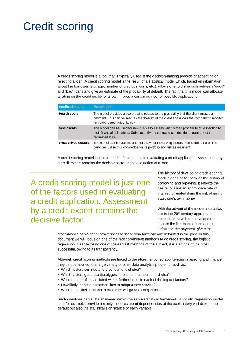
A credit scoring model is a tool that is typically used in the decision-making process of accepting or

rejecting a loan. A credit scoring model is the result of a statistical model which, based on information

about the borrower (e.g. age, number of previous loans, etc.), allows one to distinguish between "good"

and "bad" loans and give an estimate of the probability of default. The fact that this model can allocate

a rating on the credit quality of a loan implies a certain number of possible applications:

Application area Description

Health score: The model provides a score that is related to the probability that the client misses a

payment. This can be seen as the “health” of the client and allows the company to monitor

its portfolio and adjust its risk.

New clients The model can be used for new clients to assess what is their probability of respecting to

their financial obligations. Subsequently the company can decide to grant or not the

requested loan.

What drives default The model can be used to understand what the driving factors behind default are. The

bank can utilise this knowledge for its portfolio and risk assessment.

A credit scoring model is just one of the factors used in evaluating a credit application. Assessment by

a credit expert remains the decisive factor in the evaluation of a loan.

The history of developing credit-scoring

models goes as far back as the history of

borrowing and repaying. It reflects the

desire to issue an appropriate rate of

interest for undertaking the risk of giving

away one’s own money.

With the advent of the modern statistics

era in the 20th century appropriate

techniques have been developed to

assess the likelihood of someone’s

default on the payment, given the

resemblance of his/her characteristics to those who have already defaulted in the past. In this

document we will focus on one of the most prominent methods to do credit scoring, the logistic

regression. Despite being one of the earliest methods of the subject, it is also one of the most

successful, owing to its transparency.

Although credit scoring methods are linked to the aforementioned applications in banking and finance,

they can be applied to a large variety of other data analytics problems, such as:

Which factors contribute to a consumer’s choice?

Which factors generate the biggest impact to a consumer’s choice?

What is the profit associated with a further boost in each of the impact factors?

How likely is that a customer likes to adopt a new service?

What is the likelihood that a customer will go to a competitor?

Such questions can all be answered within the same statistical framework. A logistic regression model

can, for example, provide not only the structure of dependencies of the explanatory variables to the

default but also the statistical significance of each variable.

Credit scoring

A credit scoring model is just one of the factors used in evaluating a credit application. Assessment by a credit expert remains the decisive factor.


Before statistics can take over and provide answers to the above questions, there is an important step

of preprocessing and checking the quality of the underlying data. This provides a first insight into the

patterns inside the data, but also an insight on the trustworthiness of the data itself. The investigation in

this phase includes the following aspects:

What is the proportion of defaults in the data?

In order for the model to be able to make accurate forecasts it needs to see enough examples of what

constitutes a default. For this reason it is important that there is a sufficiently large number of defaults

in the data. Typically in practice, data with less than 5% of defaults pose strong modelling challenges.

What is the frequency of values in each variable in the data?

This question provides valuable insight into the importance of each of the variables. The data can

contain numerical variables (for example, age, salary, etc.) or categorical ones (education level, marital

status, etc.). For some of the variables we may notice that they are dominated by one category, which

will render the remaining categories hard to highlight in the model. Typical tools to investigate this

question are scatterplots and pie charts.

What is the proportion of outliers in the data?

Outliers can play an important role in the model’s forecasting behaviour. Although outliers represent

events that occur with a small probability and a high impact, it is often the case that outliers are a result

of system error. For example, a numerical variable that is assigned to the value 999, can represent a

code for a missing value, instead of a true numerical variable. That aside, outliers can be easily

detected by the use of boxplots.

How many missing values are there and what is the reason?

Values can be missing for various reasons, which range from missing due to nonresponse, due to drop

out of the clients, or due to censoring of the answers, or simply missing at random. Missing values

pose the following dilemma: On one hand they refer to incomplete instances of data and therefore

treatment or imputation may not reflect the exact state of affairs. However, avoiding to handle missing

values and simply ignoring them may lead to loss of valuable information. There exists a number of

ways to impute missing values, such as the expectation-maximisation algorithm.

Quality assurance

There is a standard framework around QA which aims to provide a full view on the data quality in the

following aspects: Inconsistency, Incompleteness, Accuracy, Precision, Missing / Unknown.

Data quality


Default definition

Before the analysis begins it is important to clearly state out what defines a default. This definition lies

at the heart of the model. Different choices will have an impact on what the model predicts. Some

typical choices for this definition include the cases that the client misses three payments in a row, or,

that the sum of missed payments exceeds a certain threshold.

Classification

The aim of the credit scoring model is to perform a classification: To distinguish the “good” applicants

from the “bad” ones. In practice this means the statistical models is required to find the separating line

distinguishing the two categories, in the space of the explanatory variables (age, salary, education,

etc.). The difficulty in the doing so is (i) that the data is only a sample from the true population (e.g. the

bank has records only from the last 10 years, or the data describes clients of that particular bank) and

(ii) the data is noisy which means that some of significant explanatory variables may not have been

recorded or that the default occurred by accident rather than due to the explanatory factors.

Reject inference

Apart from this, there is an additional difficulty in the development of a credit scorecard for which there

is no solution: For clients that were declined in the past the bank cannot possibly know what would

have happened if they would have been accepted. In other words, the data that the bank has refers

only to customer that were initially accepted for a loan. This means, that the data is already biased

towards a lower default-rate. This implies that the model is not truly representative for a through-the-

door client. This problem is often termed “reject inference”.

Logistic regression

One of the most common, successful and transparent ways to do the required binary classification to

“good” and “bad” is via a logistic function. This is a function that takes as input the client characteristics

and outputs the probability of default.

𝑝 =exp(𝛽0 + 𝛽1 ∙ 𝑥1 + ⋯ + 𝛽𝑛 ∙ 𝑥𝑛)

1 + exp(𝛽0 + 𝛽1 ∙ 𝑥1 + ⋯ + 𝛽𝑛 ∙ 𝑥𝑛)

where in the above

p is the probability of default

xi is the explanatory factor i

βi is the regression coefficient of the explanatory factor i

n is the number of explanatory variables

For each of the existing data points it is known whether the client has gone into default or not (i.e. p=1

or p=0). The aim in the here is to find the coefficients β0,… , βn such that the model’s probability of

default equals to the observed probability of default. Typically, this is done through maximum

likelihood.

The above logistic function which contains the client characteristics in a linear way, i.e. as 𝛽0 + 𝛽1 ∙ 𝑥1 +

⋯ + 𝛽𝑛 ∙ 𝑥𝑛 is just one way to make a logistic model. In reality, the default probability will depend on the

client characteristics in a more complicated way.

Model development


Training versus generalisation error

In general terms, the model will be tested in the following way: The data will be split into two parts. The

first part will be used for extracting the correct coefficients by minimising the error between model

output and observed output (this is the so-called “training error”).The second part is used for testing the

“generalisation” ability of the model, i.e. its ability to give the correct answer to a new case (this is the

so-called “generalisation error”).

Typically, as the complexity of the logistic function increases (from e.g. linear to higher-order powers

and other interactions) the training error becomes smaller and smaller: This means that the model

learns from the examples to distinguish between “good” and “bad”. The generalisation error is,

however, the true measure of model performance because it is testing its predictive power. This is also

reduced as the complexity of the logistic function increases. However, there comes a point where the

generalisation error stops decreasing (with more examples) with the model complexity and thereafter

starts increasing. This is the point of overfitting. This means that the model has learned to distinguish

so well the two categories inside the training data that it has also learned the noise itself. The model

has adapted so perfectly to the existing data (with all of its inaccuracies) and any new data point will be

hard to classify correctly.

Variable selection

The first phase in the model development requires a critical view and understanding on the variables

and a selection of the most significant ones. Failure to do so correctly can hamper the model’s

efficiency. This is a phase where human judgement and business intuition is critical in the success of

the model. At first instance, we seek ways to reduce the number of available variables, for example,

one can trace categorical variables where the majority of data lies within one category. Other tools from

exploratory data analysis, such as contingency tables, are useful. They could indicate how dominant a

certain category is with respect to all others. At a second instance, one can regroup categories of

variables. The motivation for this comes from the fact that there may exist too many categories to

handle (e.g. postcodes across a country), or certain categories may be linked and not able to stand

alone statistically. Finally variable significance can be assessed in a more qualitative way by using

Pearson’s chi-squared test, the Gini coefficient or the Information Value criterion.

Information Value

The Information Value criterion is based on the idea that we perform a univariate analysis: We setup a

multitude of models where there is only one explanatory variable and the response variable (the

default). Among those models, the ones that describes best the response variable can indicate the

most significant explanatory variables.

Information Value is a measure of how significant is the discriminatory power of a variable. Its definition

is

𝐼𝑉(𝑥) = ∑ (𝑔𝑖

𝑔−

𝑏𝑖

𝑏)

𝑁(𝑥)

𝑖=1

∙ 𝑙𝑜𝑔 (

𝑔𝑖

𝑔𝑏𝑖

𝑏

)

where,

N(x) is the number of levels in the variable x

gi represents the number of goods (no default) in category i of variable xi

bi represents the number of bads (default) in category i of variable xi

g represents the number of goods (no default) in the entire dataset

b represents the number of bads (default) in the entire dataset

To understand the meaning of the above expression let us go one step further. From the above it

follows that:

𝐼𝑉(𝑥) = ∑ (𝑔𝑖

𝑔)

𝑁(𝑥)

𝑖=1

∙ 𝑙𝑜𝑔 (

𝑔𝑖

𝑔𝑏𝑖

𝑏

) − ∑ (𝑏𝑖

𝑏)

𝑁(𝑥)

𝑖=1

∙ 𝑙𝑜𝑔 (

𝑔𝑖

𝑔𝑏𝑖

𝑏

) ≡ 𝐷(𝑔, 𝑏) + 𝐷(𝑏, 𝑔)


It is easy to show that 𝐷(∙,∙) is always non-negative using the so-called log-sum inequality:

𝐷(𝑔, 𝑏) ≥ (∑ (𝑔𝑖

𝑔)

𝑁(𝑥)

𝑖=1

) ∙ 𝑙𝑜𝑔 (∑

𝑔𝑖

𝑔𝑖

∑𝑏𝑖𝑏𝑖

) = 0

Since D is non-negative, i.e. D(x,y)>=0, with D(x,y)=0 if and only if x=y, the quantity D it can be used as

a measure of “distance”. Note that this is similar to the Kullback-Leibler distance.

To obtain some additional intuition concerning Information Value let us show the following four figures:

These represent two hypothetical categorical variables, named x and y. Each of these contains two

categories, say category 1 and category 2. The ratio of “good” vs “bad” is the following:

VARIABLE x GOOD BAD VARIABLE y GOOD BAD

Category 1 of x 700 75 Category 1 of y 550 80

Category 2 of x 300 25 Category 2 of y 450 20

From this example we notice that the proportion of goods versus bad in the variable x is almost the

same, while in variable y there is a more pronounced difference. Thus we can anticipate the knowledge

that a client belongs to category 1 of x will probably not give away his likelihood of future default, since

category 2 of x has the same rate of good vs bad. The contrary with variable y. Computation of the

Information Value of the two variables x and y gives: IV(x) = 0.0064 and IV(y) = 0.158. Since variable y

has a higher Information Value we say that it has better classification power. Standard practise dictates

that:

Classification power Information Value

Poor <0.15

Moderate Between 0.15 and 0.4

Strong >0.4

It is interesting to see how the same intuition can be obtained from a simple Bayesian argument.

Computing the probability of a “good” within a category (say category 1) is:

𝑃(𝐺|𝑐𝑎𝑡 1) =𝑃(𝐺, 𝑐𝑎𝑡 1)

𝑃(𝑐𝑎𝑡 1)=

𝑃(𝑐𝑎𝑡 1|𝐺)𝑃(𝐺)

𝑃(𝑐𝑎𝑡 1|𝐺)𝑃(𝐺) + 𝑃(𝑐𝑎𝑡 1|𝐵)𝑃(𝐵)

Then if 𝑃(𝑐𝑎𝑡 1|𝐺) ≈ 𝑃(𝑐𝑎𝑡 1|𝐵) we immediately have that 𝑃(𝐺|𝑐𝑎𝑡 1) ≈ 𝑃(𝐺), i.e. no extra information

can be extracted from this variable.


The aim of the modelling exercise is to find the appropriate coefficients βi for all i=0,1,…,n that lead to a

model that has two main desirable properties:

1. It fits the existing data

2. It can produce the correct probability of default on data that it has not seen before

The first of these requirements is called “Goodness-of-fit” while the second is called “Predictive

Power”. If the data sample is sufficiently large (which it is in our case) the predictive power of the

model is tested out-of-sample which means that we split the data set into a training set (used only for

model development) and a validation set (used only for model testing). We have taken the training /

validation split to be at 40%. This means that:

40% of Goods (no-default) are taken as validation data

40% of Bads (default) are taken as validation data

Such a split should be undertaken with some caution since a totally random split may result in that

some of the categories in categorical variables are not well-represented.

Goodness of Fit

If the data contained one response variable (the probability of default) and only one explanatory

variable then measuring the goodness of fit would be a trivial task: A simple graph would allow us to

inspect visually the fit. However since the dimensionality of the dataset is typically very large (of the

order of 50 variables) we have to resort to other methods. The first of these tests is a graph of the

following type:

Blue dots correspond to the points of the data set. On the x-axis we show the model prediction of the

probability of default (a real number between 0 and 1) while on the y-axis we show the actual observed

value of default (an integer value of either 0 or 1). Since we cannot easily assess the density of the

cloud of points as they overlap each other, we have “smoothed” the above set of data points by

considering, for each value across the x-axis, an average between those that have observed=0 and

those that have observed=1. The result of this smoothing process is the red line. A perfect model would

have a red line equal to the diagonal, since this would imply that if (for example) the model predicts a

PD of 30%, the observed value is also 30%. Therefore a deviation away from the diagonal indicates

that our model does not fit the data well.

Model performance


Predictive Power

There are several ways of testing the predictive power of a model, i.e. its ability to generalise the rules

it has learned from the training data set to a new (unseen) data set. The most common way is through

the computation of the histograms of the defaults versus non-defaults and subsequent inspection of

their overlap. To illustrate the point we show below a graph of two histograms: x-axis is the probability

of default while y-axis is the density of data points with a certain probability of default. In blue are the

clients which we know that have not gone in default (the “good”) while in red are the clients which we

know that have gone in default (the “bad”). We see that there is a significant overlap between the two

histograms. This implies that if the model gives a probability of default of e.g. 5% where the two

histograms are in overlap, then we cannot say with 100% certainty whether we should classify this data

point as good or as bad. In the two extremes, where PD=0 or PD=1 we see that the overlap is much

less and if the model produces a PD of that value then we can almost with 100% certainty classify the

data point as good or as bad respectively.

Choosing the correct cut-off value of the PD, below which a client is considered “good” and above

which is considered “bad”, is a matter or risk-preference and there is no simple answer as to what is

the correct cut-off value.

This leads to the ROC curve which includes in one graph the performance of the model for all possible

cut-off values. ROC stands for “Receiver Operating Characteristic”.

The ROC curve as shown below considers systematically all cut-off values for the PD from 0 to 100%.

For each cut-off value it then measures the number of Goods below the cut-off and the number of Bads

below the cut-off. It then plots these two numbers as x- and y-coordinates. A perfect model would show

a ROC curve that consists of two straight lines: From (0,0) to (0,1) and from (0,1) to (1,1), i.e. very

steep. A model with no predictive power would have a ROC curve that follows the diagonal, since that

would imply that for every cut-off value we find an equal number of goods and bads, i.e. there is a

perfect overlap in the two histograms.


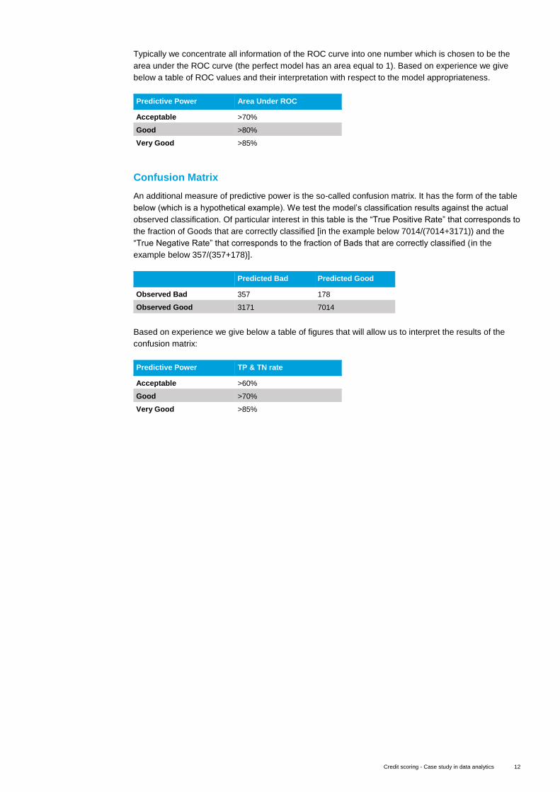
Typically we concentrate all information of the ROC curve into one number which is chosen to be the

area under the ROC curve (the perfect model has an area equal to 1). Based on experience we give

below a table of ROC values and their interpretation with respect to the model appropriateness.

Predictive Power Area Under ROC

Acceptable >70%

Good >80%

Very Good >85%

Confusion Matrix

An additional measure of predictive power is the so-called confusion matrix. It has the form of the table

below (which is a hypothetical example). We test the model’s classification results against the actual

observed classification. Of particular interest in this table is the “True Positive Rate” that corresponds to

the fraction of Goods that are correctly classified [in the example below 7014/(7014+3171)) and the

“True Negative Rate” that corresponds to the fraction of Bads that are correctly classified (in the

example below 357/(357+178)].

Predicted Bad Predicted Good

Observed Bad 357 178

Observed Good 3171 7014

Based on experience we give below a table of figures that will allow us to interpret the results of the

confusion matrix:

Predictive Power TP & TN rate

Acceptable >60%

Good >70%

Very Good >85%


There is a number of assumptions underlying the logistic regression model

𝑝 =exp(𝛽0 + 𝛽1 ∙ 𝑥1 + ⋯ + 𝛽𝑛 ∙ 𝑥𝑛)

1 + exp(𝛽0 + 𝛽1 ∙ 𝑥1 + ⋯ + 𝛽𝑛 ∙ 𝑥𝑛)

The most important of these are:

Linearity in the explanatory variables

Absence of interactions among explanatory variables

The first of these implies that inside the exponentials there are no higher-order terms, for example 𝑥12.

The second implies that there are no terms mixing the variables, for example 𝑥1 ∙ 𝑥2.These

assumptions, however, need not be necessarily true. Their validity should be tested. Testing implies

that one re-writes the logistic model slightly differently, as:

ln (𝑝

1 − 𝑝) = 𝛽0 + 𝛽1 ∙ 𝑥1 + ⋯ + 𝛽𝑛 ∙ 𝑥𝑛

The left-hand side, named the log-odds ratio, can be computed from the model. The right-hand side is

linear in the explanatory variables. This means that if the above assumptions are true one should

observe a straight line for each of the explanatory variables. If the line is not straight, then the

assumptions are not satisfied.

We illustrate this computation in the figures below. In the left figure, the log-odds ratio is approximately

straight, implying linearity is satisfied for this variable. In the right figure, the log-odds ratio is not a

straight line implying that the linearity assumption is violated.

One way to fix this problem is to create a piecewise linear function in the following way:

Model refinements


One can determine, by visual inspection or otherwise, the “knots”, which are the places where the

various linear pieces start and end. Then the construction to impose in the logistic function concerning

this variable reads:

𝑃𝑖𝑒𝑐𝑒𝑤𝑖𝑠𝑒 𝐹𝑢𝑛𝑐𝑡𝑖𝑜𝑛(𝑥) = 𝛾1 ∙ max(𝑥 − 𝐾𝑛𝑜𝑡1, 0) + 𝛾2 ∙ max(𝑥 − 𝐾𝑛𝑜𝑡2, 0) + 𝛾3 ∙ max (𝑥 − 𝐾𝑛𝑜𝑡3, 0)

The variables 𝛾𝑖 are found, as before, via Maximum Likelihood.


One of the most appealing features in logistic regression is the transparency in the interpretation of the

model. If for simplicity we consider that the model contains only one explanatory variable then we can

rewrite it as

ln (𝑝(𝑥)

1 − 𝑝(𝑥)) = 𝛽0 + 𝛽1 ∙ 𝑥1

Suppose furthermore that x is a Boolean variable. Then we obtain the two equations:

ln (𝑝(1)

1 − 𝑝(1)) = 𝛽0 + 𝛽1

ln (𝑝(0)

1 − 𝑝(0)) = 𝛽0

which together lead to the neat result:

𝑝(0)

1 − 𝑝(0)= 𝑒𝛽1

𝑝(1)

1 − 𝑝(1)

This gives the interpretation of the coefficient 𝛽1: It provides the change in the probability of default if

the variable changes by one unit. This can help us understand how the probability of default changes if

(for example) the savings capital of a client changes from 1,000 EUR to 100,000 EUR. Similarly for all

other variables.

Armed with this result we can provide further guidance to the business by giving the impact of each

individual explanatory variable to the client’s forecasted probability of default.

Model interpretation


Our team of experts provides assistance at various levels of the modelling process, from training to

design to implementation, to validation.

Deloitte’s data analytics solution team consists of high-calibre individuals with long-standing experience

in the domain of finance and data analytics.

Some examples of solutions tailored to your needs:

A managed service where Deloitte provides independent validation of your model at your request

Expert assistance with the design and implementation of your own model

A stand-alone tool

Training on the data analytics solutions, the credit scoring model, logistic regression, statistical

modelling or any other related topic tailored to your needs

Why our clients haven chosen Deloitte for advanced modelling in the Financial Services Industry:

Tailored, flexible and pragmatic solutions

Full transparency

High quality documentation

Healthy balance between speed and accuracy

A team of experienced quantitative profiles

Access to the large network of quants at Deloitte worldwide

Fair pricing

How we can help


Nicolas Castelein

Director

Enterprise Risk Services

Diegem

T: +32 2 800 2488

M: +32 498 13 57 95

E: [email protected]

Contacts

Nikos Skantzos

Director

Enterprise Risk Services

Diegem

T: +32 2 800 2421

M: + 32 474 89 52 46

E: [email protected]


Deloitte refers to one or more of Deloitte Touche Tohmatsu Limited, a UK private company limited by guarantee

(“DTTL”), its network of member firms, and their related entities. DTTL and each of its member firms are legally

separate and independent entities. DTTL (also referred to as “Deloitte Global”) does not provide services to clients.

Please see www.deloitte.com/about for a more detailed description of DTTL and its member firms.

Deloitte provides audit, tax, consulting, and financial advisory services to public and private clients spanning

multiple industries. With a globally connected network of member firms in more than 150 countries and territories,

Deloitte brings world-class capabilities and high-quality service to clients, delivering the insights they need to

address their most complex business challenges. Deloitte’s more than 200,000 professionals are committed to

becoming the standard of excellence.

This communication contains general information only, and none of Deloitte Touche Tohmatsu Limited, its member

firms, or their related entities (collectively, the “Deloitte Network”) is, by means of this communication, rendering

professional advice or services. No entity in the Deloitte network shall be responsible for any loss whatsoever

sustained by any person who relies on this communication.

© 2016. For information, contact Deloitte Belgium

http://www.deloitte.com/about

credit scoring - case study in data analytics · pdf filecredit scoring - case study in data...

Documents