credit risk stress testing: an exercise - bank of the … de estabilidad financiera diciembre de...

Credit Risk Stress Testing: An Exercise for Colombian Banks

Wilmar Cabrera RodríguezJavier Gutiérrez RuedaJuan Carlos Mendoza

Temas de Estabilidad Financiera

Diciembre de 2012, no. 73

Credit Risk Stress Testing: An Exercise for Colombian Banks∗

Wilmar Cabrera Rodríguez∗

Javier Gutiérrez Rueda†

Juan Carlos Mendoza‡

Abstract

In this paper we seek to assess the ability of banks to withstand the effects of an increase in credit risk

as a result of changes in the macroeconomic environment. To do so we estimate a credit risk model for

each loan type as a function of four macroeconomic variables commonly used in the literature. Then,

we forecast the dynamics of non-performing loans (NPL) and total loans in a stressed scenario in a

time span of 8 quarters. Using these results, we quantify the effects of the macroeconomic shock on

bank’s performance indicators, such as the NPL ratio, the return on assets, and the capital adequacy

ratio. The results suggest that most Colombian banks are able to withstand a large shock to economic

activity. We also perform a reverse stress testing to quantify how much NPL should increase in order

to bring the earnings before taxes to zero.

JEL classification: C25, D22, G21, G33

Keywords: VECX, Stress testing, non-performing loans, return on assets, capital adequacy ratio.

∗The authors would like to thank Dairo Estrada, Esteban Gómez and the staff of the Financial Stability Departmentat the Banco de la República for their useful comments and suggestions. The opinions contained herein are the soleresponsibility of the authors and do not reflect those of Banco de la República or its Board of Governors. All errors andomissions remain our own.

∗Analyst, Financial Stability Department. E-mail: [email protected]†Specialized Analyst, Financial Stability Department. E-mail: [email protected]‡Specialized Analyst, Financial Stability Department. E-mail: [email protected]


1. Introduction

Macroeconomic stress testing has become an important tool for policy makers to assess the financial sys-

tem’s resilience against unexpected shocks to the economy and the system. They are being used widely

by central banks and supervision authorities to analyze the ability of banks to withstand a crisis, to

quantify banks’ capital needs during hard times, and to evaluate how a shock may affect systemic risk.

The use of these models has gained popularity after the recent international financial crisis. The crisis

has proven the devastating effects that a shock to the financial system could have in the economy. Accor-

ding to the IMF’s World Economic Outlook, world GDP contracted by 0.6% during 2009. Advanced

economies experienced the most severe contraction (-3.6%); while emerging and developing economies

underwent a considerable reduction in their growth rate (from 6.0% in 2008 to 2.8% in 2009) (Interna-

tional Monetary Fund (2012)).

The effects of the crisis on the global unemployment rate were quite large. The International Labour

Organization (2012) estimated a 60 basis points increase in the global unemployment rate for 2009, which

translated in 24 million people loosing their jobs during that year. According to the Global Employment

Trends Report, developed economies faced the largest change in the unemployment rate, shifting from

6.1% in 2008 to 8.3% in 2009.

Global housing prices also underwent hard times due to the crisis. By regions, Europe and the U.S.

experienced the sharpest decreases in housing prices. Most European countries exhibited negative annual

growth rates for housing prices by the end of 2009. In the case of the U.S., housing prices grew at an

annual rate of -3.2% (Knight Frank Residential Research (2009)).

The financial system also endured substantial losses due to loan and securities write-downs. The

Global Financial Stability Report of April 2010 estimated bank write-downs for $2.27 trillion from the

onset of the crisis through 2010. U.S. banks were expected to have the largest losses with write-downs

reaching $885 billion; while the figure for the Euro Area and U.K. banks was $665 billion and $455 billion,

respectively (International Monetary Fund (2010)).

As of today there has not yet been a clear signal of recovery since the onset of the crisis. Advanced

economies are still struggling with low, and even negative, growth rates, rising unemployment, and dif-

ficulties in repaying their sovereign debt. According to the IMF’s chief economist, Olivier Blanchard,

it could take at least a decade to outrun the effects of the world economic crisis that began in 2008

(Blanchard (2012)).

The literature has widely studied the relation between the macroeconomy and the volume of credit

granted by the financial system. However, the research concerning the linkages among macroeconomics

and credit risk is not extensive. Alves (2005) employs a co-integrated VAR to model the dynamics of

corporate expected default frequencies (EDFs) of European industries, to which the EU banking system

is exposed, as a function of a set of macroeconomic exogenous variables.

2


Hoggarth et al. (2005) also use a VAR model to assess the relation between banks’ write-off to loan

ratio and key macroeconomic variables. The results for the aggregate model shows that there is a signi-

ficative impact of output on the write-off ratio that lasts up to six quarters after a shock. The authors

also find that there is an increase of the write-off ratio after four quarters following a shock in the annual

rate of retail price inflation and the nominal interest rate.

Wong et al. (2008) estimate two macroeconomic credit risk models using the seemingly unrelated

regression (SUR) method. The first model is used to analyze the exposure of the overall banks’ loan

portfolio to different economic sector; whereas the second does it for the mortgage portfolio. The re-

sults show that default rates of bank loans has a significative relation with Hong Kong’s real GDP, real

interest rates, real property prices and China’s real GDP. Additionally, the authors performed a macro

stress testing using adverse scenarios derived from a Monte Carlo simulation and computing a Value at

risk (VaR) for the credit loss distribution. The evidence suggest that banks are still profitable with a

VaR at a 90% confidence level; however, at a 99% confidence level they incur in high losses.

There are some previous works that analyze the case of Colombian banks. Such is the case of Gu-

tiérrez & Vásquez (2008), who estimate an error correction model to assess the relation between the

NPL ratio, economic activity, housing prices, unemployment, and interest rates. The authors find that

economic activity indicators have the strongest effects on the NPL ratio, followed by the unemployment

rate. They design a stress test as a twelve step forecast of the NPL ratio following a one time shock to

the macroeconomic variables. The results indicate that if such shock had occurred in June 2008, 88% of

the banks would have had negative profits.

The aim of this paper is to quantify and assess the severity of banks’ losses caused by increases in

the loan portfolios’ credit risk arising from unexpected shocks to the macroeconomic environment. To do

so, we estimate a VECX model to analyze the dynamics of non-performing loans and total loans against

changes in a set of four exogenous macroeconomic variables. We address the differences among loan

types by estimating a model for each of the three most important loan portfolios available in Colombia:

commercial, consumption, and mortgage loans1. We stress the loan portfolio during an eight quarter

period using a stress scenario derived from the worst paths observed for the exogenous macroeconomic

variables during the crisis of the late 1990s. The results show that banks would face the strongest impact

6 quarters after the shock begins. In this period, 11 out of 23 banks would have had negative profits and

two of them a capital adequacy ratio under the regulatory minimum.

The remainder of this paper is organized as follows. The second section describes the methodology

used to estimate the relationship between credit risk an macroeconomics variables. The third illustrates

the stress testing methodology. Section four presents the main results; whilst the final section offers the

concluding remarks.

1As of June 2012, these portfolios represent 97.2% of the loan portfolio of the Colombian financial system.

3


2. The Model

The purpose of the credit risk model is to evaluate how changes on key macroeconomic variables affect

the dynamics of two main variables relating to credit risk: non-performing loans (NPL), and total loans.

Due to the possible existence of a cointegration relationship between these variables, we use a VECX

model to assess the relationship between NPL and total loans (TL) with real GDP, real interest rates,

housing prices, and the unemployment rate. It is noteworthy that we address the huge differences among

commercial, consumption, and mortgage loans by specifying a VECX model for each loan portfolio.

We consider a model with a set of two endogenous financial variables (y) that follow an autoregressive

process of order m. In addition, there is a set of k exogenous macroeconomic variables (x) that contribute

in the explanation of the dynamics of the endogenous variables during a time span of n quarters. The

relation among these variables can be represented in vector and matrix notation as:

∆yt = µ+

m∑

i=1

Γi∆yt−i +

n∑

j=1

Ψj∆xt−j +Πyt−1 + νt (1)

where:

yt =

[

NPLt

loanst

]

;µ =

[

µ1

µ2

]

; Γi =

[

γ11,i γ12,i

γ21,i γ22,i

]

;

Ψi =

[

ψ11,i ψ12,i ψ13,i ψ14,i

ψ21,i ψ22,i ψ23,i ψ24,i

]

;xt−j =

realGDPt−j

interestratet−j

housingpricest−j

unemploymentratet−j

; Π =

[

α1β′1

α2β′2

]

; and νt =

[

ν1,t

ν2,t

]

;

where µ is a vector containing the constant terms of each equation of the endogenous variables, and Γ,

Π (the cointegration vector), and Ψ are matrices of unknown coefficients to be estimated. Lastly, ν is a

vector containing the error term of each equation. Moreover,∑m

i=1Γi∆yt−i +

∑n

j=1Ψj∆xt−j describes

the short-run dynamics of the model; whereas, Πyt−1 the long-run behavior of the variables assessed.

As mentioned, we estimate one model for each of the loan portfolios. Table 1 presents a list of the

variables used in the estimation of each of the credit risk models.

Table 1: Credit Risk Model for Each Type of Credit

Commercial Consumption Mortgage

Endogenous Commercial NPLs Consumption NPLs Mortgage NPLs

Commercial loans outstanding Consumption loans outstanding Mortgage loans outstanding

ExogenousReal GDP Real GDP Real GDP

Real interest rate Real interest rate Real housing prices

Unemployment rate Unemployment rate Unemployment rate

Source: Own calculations.

4


Before estimating the VECX model, the variables are transformed to ensure they have the desirable

properties for such models. Particularly, for NPL, TL, and GDP logarithm transformation were applied.

Also, the for unemployment rate a seasonality adjustment was implemented using the structural methods

investigated by Harvey (1989) and Harvey (1993). Additionally, for the transformed series the usual unit

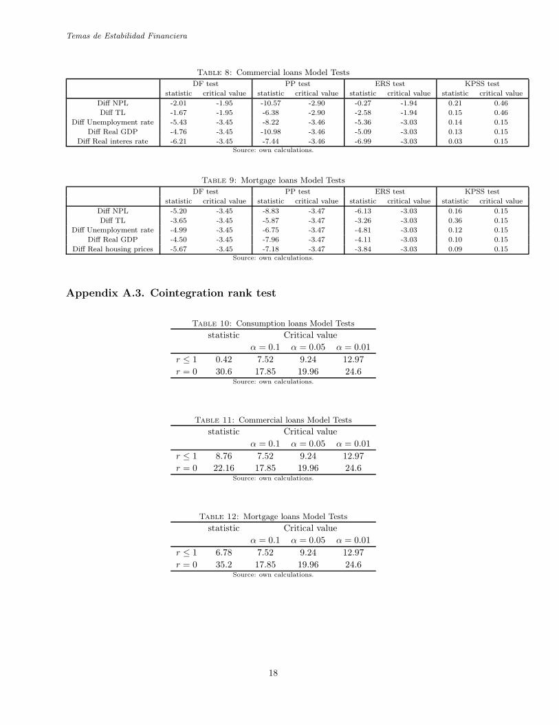
root tests were implemented and the results are presented in Appendix A2. The results of these tests,

under a significance level of 5%, indicate that the series analyzed are integrated, but can not say anything

about the order of integration.

To check the order of integration, we apply the above unit root tests on the series in their first differ-

ences. The results of these tests show that all series after this transformation are stationary. Therefore,

it can be inferred that the series analyzed have the same order of integration I(1) (The results of these

tests are displayed in Appendix A, using a significance level of 5%).

In order to find the best specification for the different VECX models, we based our choice on two

criteria: the first consist in the adjustment of the models, and the second evaluate the forecast goodness.

For the first, usual information criteria statistics were calculated, such as Hannan-Quinn (HQ), Akaike

(AIC), and Schwarz (SIC). For the second, the following measures were considered: minimum absolute

forecast error (MAFE), minimum percentage absolute forecast error (MAFPE), root minimum squared

forecast error (RMSFE), and root minimum percentage squared forecast error (RMSFPE). After that,

a set of probable models were chosen as those that minimize any of the above criteria and submit a

cointegrating vector according to the results of the Johansen test (Johansen (1995))3.

Finally, from those in the probable models group we select one for each type of loan. In this selection

process we chose the model that complies with the usual assumptions: no ARCH effects (Lütkepohl

(2006)), normality (Jarque-Bera Multivariate test, Lütkepohl (2006)), no autocorrelation (Portmanteau

test, adjusted Portmanteau test, Breusch-Godfrey LM test and Edgerton and Shukur test4), and the

most parsimonious model possible. The structures of the models chosen are presented in table 2. All

these models have a cointegrating vector (see Appendix A to observe the results of the Johansen test).

Table 2: VECX Models’ Structure

Commercial Consumption Mortgage

Endogenous four lags two lags two lags

Exogenous six lags five lags two lags


The structures of these models were used to calculate the response of the endogenous variables before

changes in exogenous variables, with the procedure known as multiplier analysis (Lütkepohl (2006)). The

paths calculated for the endogenous variables under this analysis are used in the stress testing analysis,

where this shock is translate to the banks’ balance sheet indicators.

2The test applied were Aumengted Dickey-Fuller (ADF), Phillips-Perron (PP), Kwiatkowski-Phillips-Schmidt-Shin(KPSS) and Elliot-Rothenberg-Stock (ERS).

3We search between models with a lag structure of maximum 8 lags owned and 6 of the exogenous variables.4For more details see Breusch (1978), Godfrey (1978), and Edgerton & Shukur (1999).

5


3. Stress testing

In this section we present the scheme used for stress testing and the stress test scenarios assessed. The

stress test analysis is performed individually for each of the loan portfolios analyzed with the VECX

models and, then, the results are aggregated to obtain the stress figures for the total loan portfolio5. The

stress assessment is performed in a quarterly basis during a time span of eight periods.

3.1. Stress Testing Scheme

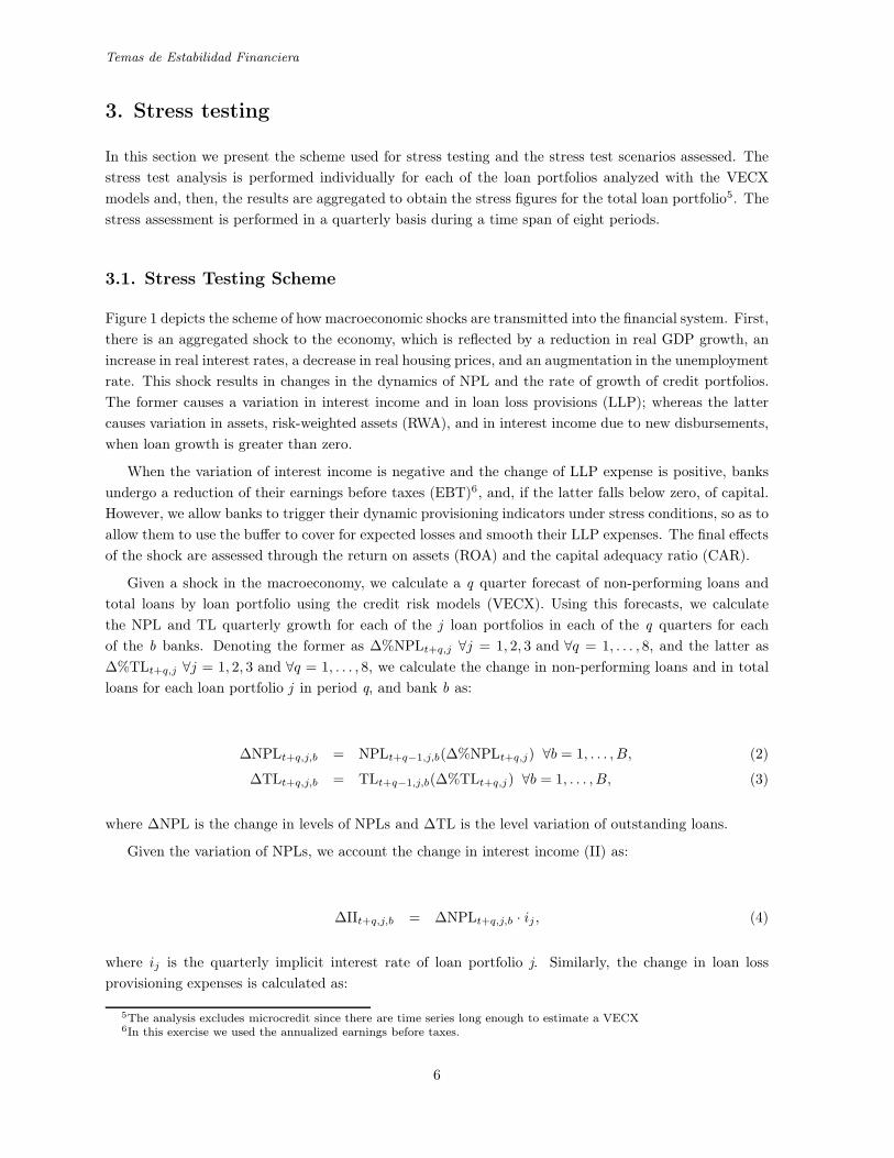
Figure 1 depicts the scheme of how macroeconomic shocks are transmitted into the financial system. First,

there is an aggregated shock to the economy, which is reflected by a reduction in real GDP growth, an

increase in real interest rates, a decrease in real housing prices, and an augmentation in the unemployment

rate. This shock results in changes in the dynamics of NPL and the rate of growth of credit portfolios.

The former causes a variation in interest income and in loan loss provisions (LLP); whereas the latter

causes variation in assets, risk-weighted assets (RWA), and in interest income due to new disbursements,

when loan growth is greater than zero.

When the variation of interest income is negative and the change of LLP expense is positive, banks

undergo a reduction of their earnings before taxes (EBT)6, and, if the latter falls below zero, of capital.

However, we allow banks to trigger their dynamic provisioning indicators under stress conditions, so as to

allow them to use the buffer to cover for expected losses and smooth their LLP expenses. The final effects

of the shock are assessed through the return on assets (ROA) and the capital adequacy ratio (CAR).

Given a shock in the macroeconomy, we calculate a q quarter forecast of non-performing loans and

total loans by loan portfolio using the credit risk models (VECX). Using this forecasts, we calculate

the NPL and TL quarterly growth for each of the j loan portfolios in each of the q quarters for each

of the b banks. Denoting the former as ∆%NPLt+q,j ∀j = 1, 2, 3 and ∀q = 1, . . . , 8, and the latter as

∆%TLt+q,j ∀j = 1, 2, 3 and ∀q = 1, . . . , 8, we calculate the change in non-performing loans and in total

loans for each loan portfolio j in period q, and bank b as:

∆NPLt+q,j,b = NPLt+q−1,j,b(∆%NPLt+q,j) ∀b = 1, . . . , B, (2)

∆TLt+q,j,b = TLt+q−1,j,b(∆%TLt+q,j) ∀b = 1, . . . , B, (3)

where ∆NPL is the change in levels of NPLs and ∆TL is the level variation of outstanding loans.

Given the variation of NPLs, we account the change in interest income (II) as:

∆IIt+q,j,b = ∆NPLt+q,j,b · ij , (4)

where ij is the quarterly implicit interest rate of loan portfolio j. Similarly, the change in loan loss

provisioning expenses is calculated as:

5The analysis excludes microcredit since there are time series long enough to estimate a VECX6In this exercise we used the annualized earnings before taxes.

6


Figure 1: Stress Testing Scheme

Aggregated shock tothe economy

↓ ∆ real GDP ↑ ∆ real interest rate ↓ ∆ real housing prices ↑ ∆ unemployementrate

∆ NPL growth ∆ Credit growth

∆ interest income ∆ loan loss provission

∆ Earnings BeforeTaxes (EBT)

∆ Core Tier 1 Ratio∆ Captial Adequacy

Ratio

.

↑ ∆ Net InterestIncome

↓ ∆ countercyclicalloan loss provission

∆ assets and riskweighted assets

If EBT is < 0

↓ ∆ Capital

If ∆CG > 0%

∆ ROA


∆LLPt+q,j,b = ∆NPLt+q,j,b · ξj − ψ% ·∆NPLt+q,j,b · ξj · ϕt, (5)

where ξj is the loan loss provisioning coefficient (LLPC) of loan portfolio j 7, ψ% is the percentage by

which LLP expense is reduced due to the use of dynamic provisions, and ϕt is an indicator variable that

is 1 when dynamic provisioning indicators are triggered and zero otherwise8.

When total loans exhibit a positive growth rate, we calculate the increase in net interest income (NII)

due to new disbursements as:

∆NIIt+q,j,b = max(0,∆TLt+q,j,b) · κj , (6)

where κj is the implicit interest margin of loan portfolio j.

7This coefficient can be calibrated in different ways, such as the ratio of specific LLP to NPLs for a given loan portfolio.However, in Colombia this ratio tends to be higher than one, due to the fact that LLP are calculated as a function of risky

loans rather than based on NPLs. Therefore, we consider the LLPCs to be equal to 1 for all loan portfolios, unless otherwisestated. By doing so, we assume that all NPLs are going to be written-off in some point of time and that banks will have toassume the cost of provisioning those loans all the way. It is noteworthy that this may lead to an overestimation of LLP,which is why bank b receives back the amount over-provisioned in t+ q − 1 when NPL’s growth is negative in t+ q.

8The regulation of the Financial Superintendence of Colombia states that ψ% is equal to 40%.

7


Given the changes in interest income, loan loss provisioning, and net interest income due to new loans,

the change in earnings before taxes for each bank is described by:

∆EBTt+q,b =

3∑

j=1

∆NIIt+q,j,b −

3∑

j=1

∆IIt+q,j,b −

3∑

j=1

∆LLPt+q,j,b, (7)

whereas the change of the EBT for the banking system is estimated as:

∆EBTt+q =

B∑

b=1

3∑

j=1

∆NIIt+q,j,b −

B∑

b=1

3∑

j=1

∆IIt+q,j,b −

B∑

b=1

3∑

j=1

∆LLPt+q,j,b. (8)

After accruing the gains and losses of each quarter, earnings before taxes are calculated for each bank

and for the banking system as:

EBTt+q,b = EBTt+q−1,b +∆EBTt+q,b, (9)

EBTt+q =

B∑

b=1

EBTt+q−1,b +

B∑

b=1

∆EBTt+q,b, (10)

(11)

∀q = 1, . . . , 8; respectively.

Using these results, we assess the impact of the macroeconomic shock on the balance sheets and

income statements of banks using three indicators: i) the return on assets (ROA), ii) the NPL ratio,

and iii) the capital adequacy ratio (CAR). The ROA is calculated on a bank-by-bank basis and for the

system for each quarter as:

ROAt+q,b =EBTt+q,b

At+q,b

, (12)

ROAt+q =

∑B

b=1EBTt+q

∑B

b=1At+q

, (13)

respectively; where At+q,b and At+q are the total assets in period t + q for bank b and for the banking

system, in the same order. Total assets are forecasted for each period assuming the same growth rate of

the loan portfolio as follows:

At+q,b = At+q−1,b ·∆%TLt+q,b, (14)

At+q =

B∑

b=1

At+q,b, (15)

8


where At+q,b is the total assets of bank b in period t+ q, ∆%TLt+q,b is the loan portfolio growth in t+ q,

which is calculated as a weighted average of the j types of credit9.

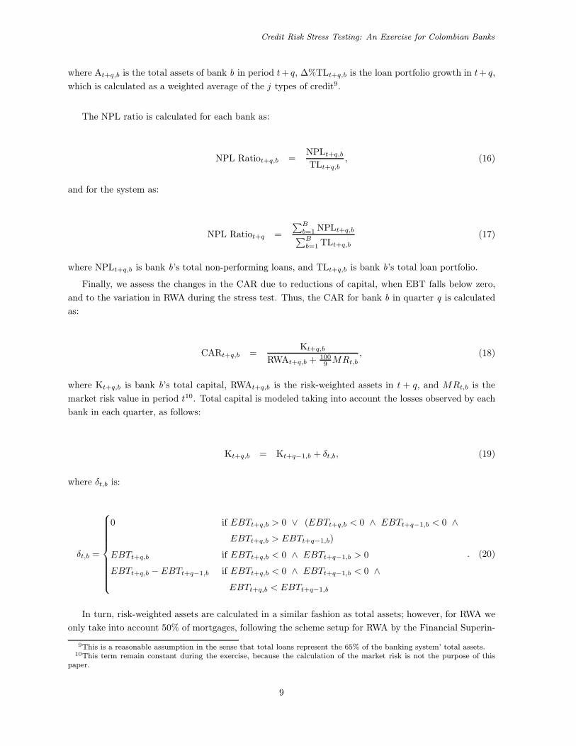
The NPL ratio is calculated for each bank as:

NPL Ratiot+q,b =NPLt+q,b

TLt+q,b

, (16)

and for the system as:

NPL Ratiot+q =

∑B

b=1NPLt+q,b

∑B

b=1TLt+q,b

(17)

where NPLt+q,b is bank b’s total non-performing loans, and TLt+q,b is bank b’s total loan portfolio.

Finally, we assess the changes in the CAR due to reductions of capital, when EBT falls below zero,

and to the variation in RWA during the stress test. Thus, the CAR for bank b in quarter q is calculated

as:

CARt+q,b =Kt+q,b

RWAt+q,b +100

9MRt,b

, (18)

where Kt+q,b is bank b’s total capital, RWAt+q,b is the risk-weighted assets in t + q, and MRt,b is the

market risk value in period t10. Total capital is modeled taking into account the losses observed by each

bank in each quarter, as follows:

Kt+q,b = Kt+q−1,b + δt,b, (19)

where δt,b is:

δt,b =

0 if EBTt+q,b > 0 ∨ (EBTt+q,b < 0 ∧ EBTt+q−1,b < 0 ∧

EBTt+q,b > EBTt+q−1,b)

EBTt+q,b if EBTt+q,b < 0 ∧ EBTt+q−1,b > 0

EBTt+q,b − EBTt+q−1,b if EBTt+q,b < 0 ∧ EBTt+q−1,b < 0 ∧

EBTt+q,b < EBTt+q−1,b

. (20)

In turn, risk-weighted assets are calculated in a similar fashion as total assets; however, for RWA we

only take into account 50% of mortgages, following the scheme setup for RWA by the Financial Superin-

9This is a reasonable assumption in the sense that total loans represent the 65% of the banking system’ total assets.10This term remain constant during the exercise, because the calculation of the market risk is not the purpose of this

paper.

9


tendence of Colombia.

The banking system’s capital adequacy ratio is calculated by adding all components across banks as

follows:

CARt+q =

∑B

b=1Kt+q,b

∑B

b=1RWAt+q,b +

100

9

∑B

b=1MRt,b

, (21)

3.2. Stress Testing Exercises

In this section we present the exercises that we designed for conducting the stress test. The first exercise

tries to replicate the worst events observed during the Colombian economic crisis of the late 1990’s. The

second exercise is a reverse stress test with which we would like to assess what is the change in NPL

needed to run down the profits of the Colombian banking system to zero.

Figure 2: Stress Scenario

A. GDP Growth(%) B. Unemployment Rate (%)

-8.0

-6.0

-4.0

-2.0

0.0

2.0

4.0

6.0

8.0

1994 1996 1998 2000 2002 2004 2006 2008 2010 2012 2014

6.0

8.0

10.0

12.0

14.0

16.0

18.0

20.0

22.0

1994 1996 1998 2000 2002 2004 2006 2008 2010 2012 2014

C. Real Housing Prices D. Real Interest Rate (%)

2.8

3.2

3.6

4.0

4.4

4.8

5.2

1994 1996 1998 2000 2002 2004 2006 2008 2010 2012 2014

-4.0

0.0

4.0

8.0

12.0

16.0

1994 1996 1998 2000 2002 2004 2006 2008 2010 2012 2014

Source: DANE, and own calculations.

Figure 2 illustrates the hypothetical trajectories that the exogenous variables would take in the sce-

nario considered in the first exercise, beginning in June 2012. As is shown in the figures, real GDP is

assumed to present a sharp drop during late 2012 and mid 2013; reaching its minimum growth in June

2013 (-7.0% y/y). Real housing prices would present a considerable contraction, falling by 24% in a seven

quarter time span. The scenario also assumes an increase in the unemployment rate, which reaches a

10


peak of 19.3% five quarters after the shock starts. Finally, we try to replicate the interest rate hike during

late 1998, reaching a maximum of 11.4% four quarters after the first shock hits. It is noteworthy that

this hike in the interest rate is not likely to occur again during a crisis due to a change in the monetary

regime11.

4. Results

The stress test exercises were performed based on the Colombian banking sector’s balance sheet as

of June 2012. For the first exercise we calculate the effects of an adverse macroeconomic scenario on

different financial indicators such as the non-performing loans ratio (NPL ratio), ROA, and CAR, for a

two year time horizon. In the second exercise, we find the NPL growth rate in a two year horizon that

runs down the profits of the banking system to zero, for different credit growths.

4.1. Stress testing results

Given a scenario like the one described in the previous section, the banking sector’s NPL ratio would

increase from 3.3% in June 2012 to 9.2% in December 2013, at which time it would experience its highest

value. Subsequently, the indicator would begin to decrease, as the macroeconomic environment improves,

reaching 7.1% in June 2014 (Figure 3).

Figure 3: Shock’s effect over the NPL ratio (%)

2.0

4.0

6.0

8.0

10.0

12.0

14.0

16.0

1994 1996 1998 2000 2002 2004 2006 2008 2010 2012 2014

Source: Financial Superintendence of Colombia, and own calculations.

The increase in the NPL ratio would generate a reduction in the EBT of COP$6.0 billion (b) during

the two years of the shock -i.e., the banking system’s EBT would fall from COP$8.2 b in June 2012 to

COP$2.3 b, two years after. Additionally, 11 banks would present negative EBT during the exercise,

while 7 banks would finish with negative EBT. This decrease in the EBT would cause a reduction in the

banking system’s ROA of 1.9 percentage points (pp), changing from 2.6% in June 2012 to 0.7% two years

after (Figure 4, Panel A). It is noteworthy that this indicator would register its minimum value (-0.4%) in

11Back then, Colombia was under an exchange rate band regime, and after the crisis such regime was changed to inflationtargeting.

11


December 2013. Importantly, despite the magnitude of the shock, the aggregated banking sector’s EBT

is positive at the end of the exercise.

Table 3: Effects of the Shock on Bank’s Income Statement

Commercial∗ Consumption∗ Mortgage∗ Total∗ Stressed EBT∗

EBT - June 2012 8.23 8.23 8.23 8.23 8.23

t+1 -0.24 -0.62 -0.42 -1.28 6.95

t+2 -0.36 -0.81 -0.66 -1.74 6.49

t+3 -0.77 -1.08 -1.28 -2.96 5.27

t+4 -1.03 -1.37 -1.63 -4.03 4.41

t+5 -2.59 -3.39 -2.86 -8.84 -0.40

t+6 -3.52 -3.15 -2.95 -9.62 -1.18

t+7 -3.65 -2.29 -3.05 -8.99 -0.50

t+8 -2.41 -1.24 -2.64 -6.29 2.27

∆ % EBT in t+6 42.8% 38.2% 35.9% 100%+ -8.63

∆ % EBT in t+8 29.2% 15.1% 32.1% 76.4% -5.96

∗ Billon COP.

EBT: Earnings before taxes.

Source: Financial Superintendence of Colombia, own calculations.

Additionally, we calculate the effects on the CAR for the banking sector. Despite the size of the

shock, this indicator would not present significant changes, going from 15% in June 2012 to 14.9%, two

years later. These values are higher than the regulatory minimum (9%). This result could be explain

because the RWA do not have a significant change during the exercise. The reason for this is explained in

more detail in the following section. Moreover, no bank finishes with a CAR lower than 9%; nonetheless,

during the exercise two entities register a CAR lower than the regulatory minimum, although is just for

two quarters (Figure 4, Panel B).

Figure 4: Shock’s effect over ROA and CAR (%)

A. ROA B. CAR

-4.0

-3.0

-2.0

-1.0

0.0

1.0

2.0

3.0

4.0

1994 1996 1998 2000 2002 2004 2006 2008 2010 2012 2014

8.0

9.0

10.0

11.0

12.0

13.0

14.0

15.0

16.0

1994 1996 1998 2000 2002 2004 2006 2008 2010 2012 2014


Figure 5 shows the number of banks that would present a negative ROA or a CAR lower than the

regulatory minimum during the exercise. Six quarters after the stress exercise begins, the banking system

would have the worst performance, as with 11 banks presenting a negative ROA and two a CAR lower

than 9%. In the case of the latter, it is noteworthy that in spite of the CAR been lower than 9% in some

quarters, both would finish the exercise with a CAR higher than the regulatory minimum.

12


Figure 5: Number of Banks with Negative Profit and Under Regulatory CAR

0

2

4

6

8

10

12

III IV I II III IV I II

2012 2013 2014

Banks under regulatory CAR Banks with negative profits


4.2. Reverse stress testing results

We performed a reverse stress testing exercise to find out what is the nominal quarterly growth of

NPL that is needed to run down the banking sector’s profits to zero, assuming different nominal quarterly

growth for the total loans portfolio. As expected, the greater the growth of total loans, the bigger the

growth of NPL needed to run down profits (figure 6). Particulary, if we suppose that the quarterly growth

of total loans for the next two years is equal to the growth observed in the last two years (5.0%), the

NPL quarterly growth needed to run down the profits is 13.6%. This value is much bigger than the one

registered in the last two years (1.0%). This result suggests that given the current conditions of the

Colombian financial system, an event like the one described above has a low probability of occurrence.

Figure 6: Reverse stress exercise

10

12

14

16

18

20

22

24

0 3 5 8 10 13 15 18 20 22 25 27 30

Total loans nominal quarterly growth (%)

NP

L n

om

ina

l q

ua

rte

rly g

row

th (

%)

(5.0, 13.6)


13


Additionally, based on this scenario where NPL quarterly growth is 13.6% while for total loans is

5.0%, we observed that the NPL ratio increases from 3.3% in June 2012 to 6.1%, two years later. We also

calculate the effects on the CAR. Between June 2012 and 2014, this indicator would change from 15.0%

to 10.4% and 10 of 23 banks analyzed would present a CAR lower than the regulatory minimum12.

In spite of the differences in the construction of the two exercise, it is important to note the large

differences in the effects obtained on the CAR. The main reason for this is the Colombian definition

of the risk weighted assets (RWA). Basically, in Colombia the RWA are not calculated by a risk-based

approach13, where if the loan portfolio becomes more risky the RWA increase, even if the size of the

portfolio does not change. By contrast, its calculation is based on the assets’ exposure and the risk

weights are fixed by asset type. Therefore, although there is no great difference in the NPL growth

between the two exercises, the average growth of total loans is very different, and this affects the forecast

of the RWA. While in the first exercise the average nominal quarterly growth for the total loans is 0.75%,

in the second exercise it is 5% and this explains the greater fall in the CAR for the reverse stress exercise.

5. Conclusions

In this paper we develop a stress testing methodology for the banking system. Using a VECX model

we estimate the relation between NPL, total loans and different macroeconomic variables such as GDP

growth, the unemployment rate, the interest rate and housing prices. With these estimations, we perform

a stress exercise to find out how an adverse macroeconomic scenario, like the one observed in the late 90s

in Colombia, affects the performance of the banking system in a time horizon of two years. These effects

are evaluated through distinct financial indicators such as ROA, NPL ratio and CAR.

The results show that, despite the great magnitude of the shock, the banking sector EBT remain

positive at the end of the exercise. Additionally, the effects on the CAR are not significant, and all

entities finalize the exercise with this indicator above the regulatory minimum. Nonetheless, the banks

would face the strongest impact 6 quarters after the shock begins; in this period 11 out of 23 banks would

have had negative profits and two of them a CAR under the regulatory minimum.

The reverse stress exercise shows that, given a 5% quarterly nominal growth of total loans, the NPL

quarterly growth must be 13.6% during two years to run down the banking system’s profits to zero. In

contrast with the stress exercise, in this one the reduction on the banking system’s CAR would be higher

and 10 banks would finish the exercise with a CAR lower than the regulatory minimum (9%).

Since the latest financial crisis, stress testing exercises have become very important. In Colombia there

is not a basis or a legal framework to perform these exercises that establish macro-financial links, and

those that have been used tend to be too simplified. This framework helps to improve the stress exercises

using sophisticated but accessible tools. Therefore, it constitutes a first advance in the development of

this kind of stress testing exercises in Colombia.

12The graphs of the NPL ratio and the CAR for this exercise are presented in Appendix B.13Like the Quasi-IRB approach commonly used. See Schmieder and others (2011).

14


As a policy recommendation, we think that this kind of framework can be used by supervisors,

regulators, and financial institutions in Colombia, in order to evaluate the resilience of the banking

sector, and any particular entity, to face an adverse macroeconomic scenario. It is noteworthy that

the framework developed in this paper is flexible enough to be used in different types of stress testing

exercises.

15


References

Alves, I. (2005), Sectoral Fragility: Factors and Dynamics , in Bank for International Settlements , ed.,

‘Investigating the Relationship Between the Financial and Real Economy’, Vol. 22 of BIS Papers

chapters, Bank for International Settlements , pp. 450–80.

Blanchard, O. (2012), ‘Blanchard: Eurozone Integration Needs to Go Forward or Go Back, But It Can’t

Stay Here’, (Interview published in Portfolio.hu) .

Breusch, T. (1978), ‘Testing for Autocorrelation in Dynamic Linear Models’, Australien Economic Papers

(17), 334–355.

Edgerton, D. & Shukur, G. (1999), ‘Testing Autocorrelation in a System Perspective’, Econometric

Reviews (18), 343–386.

Godfrey, L. (1978), ‘Testing for Higher Order Serial Correlation in Regression Equations when the Re-

gressors Include Lagged Dependent Variables’, Econometrica (46), 1303–1310.

Gutiérrez, J. & Vásquez, D. (2008), ‘Un Análisis de Cointegración para el Riesgo de Crédito ’, Temas de

estabilidad financiera .

Harvey, A. (1989), ‘Forecasting, structural time series models and the kalman filter’, Cambridge University

Press .

Harvey, A. (1993), Time series models , Harvester Wheatsheaf (2nd Edition).

Hoggarth, G., Sorensen, S. & Zicchino, L. (2005), Stress Tests of UK Banks Using a VAR Approach ,

Bank of England working papers 282, Bank of England.

International Labour Organization (2012), ‘Global Employment Trends’, (Geneva: International Labour

Organization) .

International Monetary Fund (2010), ‘Global Financial Stability Report ’, (Washington: International

Monetary Fund) .

International Monetary Fund (2012), ‘World Economic Outlook’, (Washington: International Monetary

Fund) .

Johansen, S. (1995), Likelihood-based Inference in Cointegrated Vector Autoregressive Models , Oxford

University Press.

Knight Frank Residential Research (2009), ‘News Release ’, (London: Knight Frank LLP) .

Lütkepohl, H. (2006), New Introduction to Multiple Time Series Analysis , Berlin: New York: Springer.

Wong, J., Choi, K. & Fong, T. (2008), ‘A Framework for Stress Testing Banks’ Credit Risk’, The Journal

of Risk Model Validation 2(1), 3–23.

16


Appendix A. VECX Model Tests

Appendix A.1. Unit Root Tests with variables in levels

Table 4: Consumption loans Model Tests

DF test PP test ERS test KPSS test

statistic critical value statistic critical value statistic critical value statistic critical value

NPL 0.24 -1.95 -1.50 -2.90 -2.07 -1.94 0.32 0.46

TL 1.19 -1.95 0.48 -2.90 0.39 -1.94 0.89 0.46

Unemployment rate -0.19 -1.95 -1.14 -2.90 -1.06 -1.94 0.54 0.46

Real GDP 4.65 -1.95 0.72 -2.90 3.81 -1.94 2.14 0.46

Real interes rate -3.60 -3.45 -3.12 -3.46 -3.76 -3.03 0.17 0.15Source: own calculations.

Table 5: Commercial loans Model Tests



NPL 0.05 -1.95 -1.93 -2.90 -1.52 -1.94 0.37 0.46

TL 1.13 -1.95 -0.20 -2.90 -0.69 -1.94 1.61 0.46


Real GDP 4.65 -1.95 0.72 -2.90 3.81 -1.94 2.14 0.46

Real interes rate -3.60 -3.45 -3.12 -3.46 -3.76 -3.03 0.17 0.15Source: own calculations.

Table 6: Mortgage loans Model Tests



NPL -0.03 -1.95 -1.76 -2.90 -0.77 -1.94 0.42 0.46

TL -0.86 -1.95 -0.76 -2.90 -0.77 -1.94 1.39 0.46


Real GDP 3.81 -1.95 1.12 -2.90 2.83 -1.94 1.79 0.46

Real housing prices -2.45 -3.45 -0.60 -3.47 -0.87 -3.03 0.44 0.15Source: own calculations.

Appendix A.2. Unit Root tests with variables in differences




Diff NPL -2.12 -1.95 -9.94 -2.90 -0.40 -1.94 0.17 0.46

Diff TL -4.92 -3.45 -7.19 -3.46 -4.88 -3.03 0.15 0.15

Diff Unemployment rate -5.43 -3.45 -8.22 -3.46 -5.36 -3.03 0.14 0.15

Diff Real GDP -4.76 -3.45 -10.98 -3.46 -5.09 -3.03 0.13 0.15

Diff Real interes rate -6.21 -3.45 -7.44 -3.46 -6.99 -3.03 0.03 0.15Source: own calculations.

17





Diff NPL -2.01 -1.95 -10.57 -2.90 -0.27 -1.94 0.21 0.46

Diff TL -1.67 -1.95 -6.38 -2.90 -2.58 -1.94 0.15 0.46


Diff Real GDP -4.76 -3.45 -10.98 -3.46 -5.09 -3.03 0.13 0.15

Diff Real interes rate -6.21 -3.45 -7.44 -3.46 -6.99 -3.03 0.03 0.15Source: own calculations.




Diff NPL -5.20 -3.45 -8.83 -3.47 -6.13 -3.03 0.16 0.15

Diff TL -3.65 -3.45 -5.87 -3.47 -3.26 -3.03 0.36 0.15


Diff Real GDP -4.50 -3.45 -7.96 -3.47 -4.11 -3.03 0.10 0.15

Diff Real housing prices -5.67 -3.45 -7.18 -3.47 -3.84 -3.03 0.09 0.15Source: own calculations.

Appendix A.3. Cointegration rank test


statistic Critical value

α = 0.1 α = 0.05 α = 0.01

r ≤ 1 0.42 7.52 9.24 12.97

r = 0 30.6 17.85 19.96 24.6Source: own calculations.



α = 0.1 α = 0.05 α = 0.01

r ≤ 1 8.76 7.52 9.24 12.97




α = 0.1 α = 0.05 α = 0.01

r ≤ 1 6.78 7.52 9.24 12.97


18


Appendix B. Reverse Stress testing Results

Figure 7: Shocks’ effect over the NPL ratio (%)

2.0

4.0

6.0

8.0

10.0

12.0

14.0

16.0

1994 1996 1998 2000 2002 2004 2006 2008 2010 2012 2014

NPL ratio NPL ratio Stress test NPL ratio Reverse Stress test


Figure 8: Shocks’ effect over the CAR (%)

8.0

9.0

10.0

11.0

12.0

13.0

14.0

15.0

16.0

1994 1996 1998 2000 2002 2004 2006 2008 2010 2012 2014

CAR Stress test CAR Reverse Stress test CAR


19

credit risk stress testing: an exercise - bank of the … de estabilidad financiera diciembre de...

Documents