Credit Price Optimisation withinRetail Banking

S.E. Terblanche∗ T. De la Rey

Centre for Business Mathematics and Informatics

North-West University (Potchefstroom), South Africa

{fanie.terblanche,tanja.delarey}@nwu.ac.za

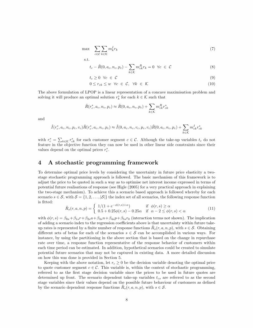
Abstract

The willingness of a customer to pay for a product or service is mathematically capturedby a price elasticity model. The model relates the responsiveness of customers to a change inthe quoted price. In addition to overall price sensitivity, adverse selection could be observedwhereby certain customer segments react differently towards price changes. In this paperthe problem of determining optimal prices to quote prospective customers in credit retail isaddressed such that the interest income to the lender will be maximised while taking pricesensitivity and adverse selection into account. For this purpose a response model is suggestedthat overcomes non-concavity and unrealistic asymptotic behaviour which allows for a lineari-sation approach of the non-linear price optimisation problem. A two-stage linear stochasticprogramming formulation is suggested for the optimisation of prices while taking uncertaintyin future price sensitivity into account. Empirical results are based on real data from a financialinstitution.

1 Introduction

In recent years there has been a significant shift by some industries to move away from cost basedpricing, where the price of a product or service is based on the cost plus some fixed profit margin,to a more flexible demand-based pricing strategy, see Skugge (2011). Demand-based pricing is doneby taking into account the willingness of a customer to pay for a product or service, i.e. priceelasticity. The responsiveness of the quantity demanded of a product or service to a change inits price is a measure of elasticity and it is commonly referred to as a price response function.Examples of typical price response functions are the linear, the constant-elasticity and the s-shapedprice response function, see Phillips (2005).

Knowing more about the customer would likely improve the predictive power of a responsefunction. Cross and Dixit (2005) state that the key to customer-centric pricing is to set prices thataccurately reflect the perceived value of products per customer segment, where a customer segmentis a grouping of customers having similar characteristics and product preferences. In Agrawal andFerguson (2007) bid-response models are presented for customised business-to-business bid pricingand they show that by making use of customer segmentation an increase in profits can be expected.In Phillips (2012) a pricing approach is suggested where price levels are determined per customersegment while taking price sensitivity into account.

In retail banking, specifically consumer credit, the pricing approach followed for many years waslimited to risk-based pricing, see Edelberg (2006). The dependence on risk-based pricing could beattributed to the uncertainty in the expected revenue and costs associated with consumer credit.In Caufield (2012), however, it is argued that risk-based pricing is the lending industry’s version ofcost-based pricing and that an increase in profit of between 10-25 percent could be expected with

∗Corresponding author

1

a profit-based pricing approach. Such an approach would typically combine risk-based pricing anddemand-based pricing in an attempt to maximise profits.

The problem being addressed in this study is the pricing of consumer credit products in retailbanking. In addition to general price sensitivity, adverse selection is an important characteristic inretail credit that is likely to have a significant impact on pricing, see Stiglitz and Weiss (1981). Thephenomenon in retail credit where low risk customers are more sensitive to an increase in pricescompared to high risk customers can be attributed to adverse selection. Therefore, according toThomas (2009), adverse selection needs to be taken into account as part of risk-based pricing sinceit influences the interaction between the quality of the customers and the probability of them takingup credit products. In Huang and Thomas (2009) a quantification for adverse selection is givenwithin the context of risk pricing and they show how errors in the risk scoring models could effectprofitability.

The literature contains empirical evidence of the existence of price elasticity and adverse selectionin retail credit. Specifically, in Park (1997) results indicate that for the credit card industry adecrease in demand is associated with an increase in price. This is also the case for the creditindustries in less developed economies, see Karlan and Zinman (2008). The study by Ausubel (1999)also showed clear evidence of adverse selection within the credit card industry and in Phillips andRaffard (2009) evidence is provided of adverse selection in the US sub-prime auto lender market.In Einav et al. (2012) an empirical model of demand for subprime credit is developed that takesadverse selection into account. Applying their model on detailed cost data they find that optimalprices dictate lowering down payment requirements for low risk customers and increasing it for highrisk customers.

Most of the literature on the topic of pricing, as outlined above, focusses on determining thefactors that influence price setting and the relationships that may exist between consumer behaviourand pricing. Only recently have there been efforts to formalise the retail credit price optimisationproblem and the challenges faced with obtaining optimal solutions. In Phillips (2013) the pricingproblem for credit consumers entails determining optimal prices per pricing segment according to anobjective function that combines the net interest income with price sensitivity. The log-concavityproperty of the said objective function allows for the efficient generation of optimal prices providedthat any additional side constraints preserve convexity of the feasible region. No numerical resultsare presented in that paper. In the paper by Oliver and Oliver (2012) a numerical algorithm isprovided to find optimal prices to maximise return on equity by considering price response anddefault risk. Their approach is based on the solution of non-linear differential equations.

The price optimisation model considered in this paper is based on the work by Phillips (2013) andtakes uncertainty in future price sensitivity into account. To the best of our knowledge uncertaintyin future price sensitivity has not been considered previously in any study concerned with retailcredit price optimisation. Furthermore, a response model is suggested that overcomes non-concavityand unrealistic asymptotic behaviour. This allows for a linearisation of the retail price optimisationproblem making it more tractable for a stochastic linear programming approach, see Higle (2005).The empirical results presented in this paper are based on real data from the South African retailbank Absa, a subsidiary of Barclays Bank Plc.

In the next section empirical evidence is provided that support the use of a stochastic program-ming framework. In Section 3 the income function used to approximate the net present interestincome with is introduced and details are provided of the newly proposed response function. Alinear approximation of the newly proposed response function is provided and incorporated into alinear programming model for solving the credit price optimisation problem with multiple customersegments. In Section 4 the basic problem is extended to cater for uncertainty in future price sen-sitivity by formulating the credit price optimisation problem as a linear stochastic programmingproblem. Empirical results are provided in Section 5 that highlights the benefits of following astochastic programming approach based on real data. Finally, summary remarks and a conclusion

2

are provided in Section 6.

2 Price sensitivity and adverse selection

The optimisation problem addressed in this paper is solving the retail credit price optimisationproblem by taking uncertainty in future price sensitivity into account. That is, the output fromsolving this problem are the optimal prices that will be quoted to prospective customers, i.e theloan interest rates, such that the interest income to the lender, discounted with the effect of priceelasticity and adverse selection, will be maximised. In this section evidence of the existence of priceelasticity and adverse selection will be provided and a case will be made for using a stochasticprogramming framework for solving retail credit price optimisation problem.

To illustrate the effect of price sensitivity and the effect of adverse selection, empirical tests wereperformed using data obtained from a financial institution in South Africa over a period of threeyears. The variables contained within the data set included:

� whether a customer took up a loan (Y = 1) or not (Y = 0)

� the quoted interest rate (r)

� the repurchase rate (r0)

� the loan amount (a)

� the loan term (n)

� the probability of default (p)

� the loan application date.

The probability of a customer taking up a loan is expressed as the following response functionobtained from fitting a logistic regression model:

R(r, a, n, p) =1/(

1 + e(−(β0+β1r+β2a+β3n+β4p+β5r0)))

(1)

with β1 to β5 the regression coefficients that are estimated through the maximum likelihood method.Note that for ease of illustration interaction terms between the different variables have been omitted.Furthermore, instead of following the customary approach of modelling the margin r − r0, therepurchase rate r0 is considered separately and is shown in the results to feature in some of theinteraction terms. The response function R(r, a, n, p) gives the probability that a customer with aprobability of default of p will take up a loan of size a, term of n and with a quoted price of r,provided that the current repurchase rate is r0. In subsequent sections the notation R(r, a, n, p)will be used to obtain a two dimensional response function in terms of the variable r by supplyingconstant values for a, n and p to the logistic regression model (1).

A stepwise logistic regression was performed (p-value of 5%) and a c-statistic of 0.608 wasobtained. Although a perfect model would have yielded a c-statistic of one it should be noted thatthe data set under consideration is limited in the number of variables and with additional variablescapturing information such as demographics, application turn-around time, macro economic factors,etc. an improved c-statistic would most likely be possible.

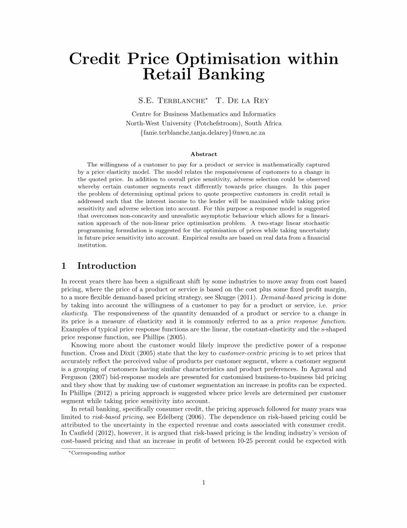
Figure 1 shows the response graph of price vs take-up generated from the response functionR(r, a, n, p) by substituting averages from the data set for a, n and p. The graph clearly shows thatprice elasticity exists since lower take-up rates are associated with an increase in price. Adverseselection is a term used to refer to a market process where ”bad” results occur when buyers andsellers have asymmetric information: the ”bad” products or customers are more likely to be selected.

3

0.10

0.20

0.30

0.40

0.50

0.60

0.70

0.80

0.90

1.00

Takeuppercentage

Rate (r)

Figure 1: Response graph of price vs take-up

0.10

0.20

0.30

0.40

0.50

0.60

0.70

0.80

0.90

1.00

Takeuppercentage

Rate (r)

High Risk

Low Risk

Figure 2: Response graph of price vs take-up for different risk categories

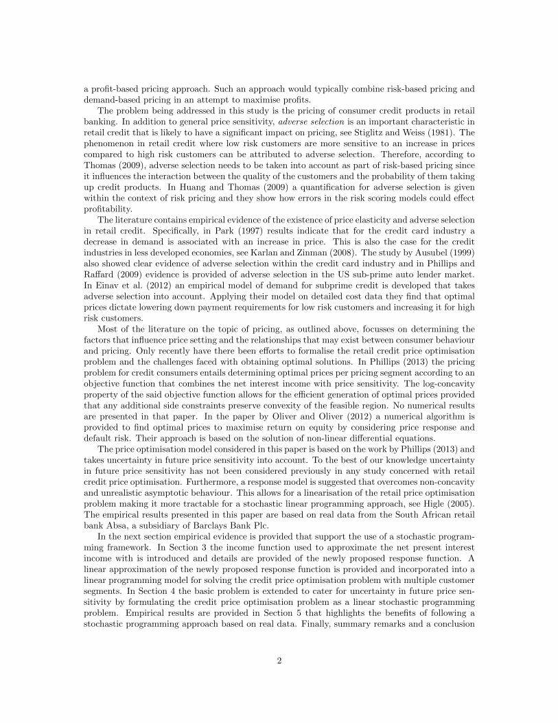
The resulting effect in credit retail is that low risk customers are more sensitive to an increase inprices compared to high risk customers. To illustrate the effect of adverse selection different levelsof probability of default (p) were substituted into the response function R(r, a, n, p) for low riskand high risk customers respectively. Figure 2 shows that the take-up for high risk customers washigher compared to low risk customers for the same quoted price, implying that adverse selectiondoes indeed exist for this data set.

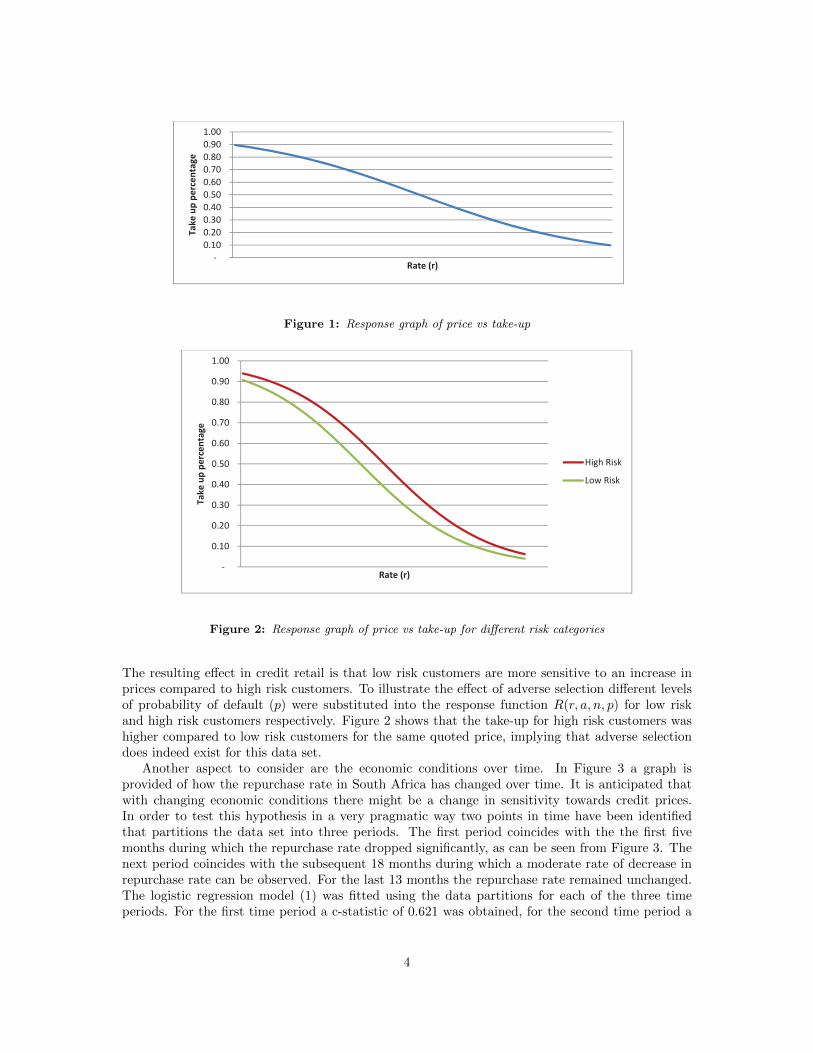
Another aspect to consider are the economic conditions over time. In Figure 3 a graph isprovided of how the repurchase rate in South Africa has changed over time. It is anticipated thatwith changing economic conditions there might be a change in sensitivity towards credit prices.In order to test this hypothesis in a very pragmatic way two points in time have been identifiedthat partitions the data set into three periods. The first period coincides with the the first fivemonths during which the repurchase rate dropped significantly, as can be seen from Figure 3. Thenext period coincides with the subsequent 18 months during which a moderate rate of decrease inrepurchase rate can be observed. For the last 13 months the repurchase rate remained unchanged.The logistic regression model (1) was fitted using the data partitions for each of the three timeperiods. For the first time period a c-statistic of 0.621 was obtained, for the second time period a

4

0.00%

2.00%

4.00%

6.00%

8.00%

10.00%

12.00%

14.00%

Repurchase

rate

Time

Figure 3: Repurchase rate over time

0

0.1

0.2

0.3

0.4

0.5

0.6

0.7

0.8

0.9

1

Takeuppercentage

Rate (r)

Time period 1

Time period 2

Time period 3

Figure 4: Response graph of price vs take-up for different time periods

c-statistic of 0.618 was obtained and for the last time period a c-statistic of 0.6 was obtained.Figure 4 provides a graph for each of the response functions fitted to each of the time periods.

The lack of sensitivity towards price increases in the first period could be attributed to an opti-mistic economic outlook due to the steep decline in repurchase rate within a short period of time.Irrespective of the reason for this phenomenon, it is clear that economic conditions could have aneffect on price elasticity. Empirical evidence (not reported here) also suggest this to be true foradverse selection. It is, therefore, a reasonable approach to take potential future price sensitivityinto account when determining prices to be quoted to prospective customers. For instance, if wehave to determine prices at this point in time we could consider the three response graphs depictedin Figure 4 as potential future scenarios with respect to price sensitivity. That is, in the near futurethe current repurchase rate level may either drop significantly, or only moderately or remain un-changed as was historically the case. Note that the proposed optimisation approach below will allowus to also incorporate potential future scenarios that are not captured as part of the historic data.For instance, another potential future scenario to consider might be that the current repurchaserate will increase in the future, especially if it is currently at a low level.

5

In view of the above, the optimization question at hand is, therefore, to determine optimal pricelevels by considering the uncertainty in future price elasticity which could be represented by a finiteset of potential future scenarios. Preceding the details of the proposed model that addresses thisproblem, the fundamental building blocks of the credit price optimisation problem is set out below.

3 A concave linear approximation of the objective function

Let the probability of default for a customer be denoted by p and the loss given default by δ.Furthermore, let a be the loan amount, n the term (in months) and r the price (annual interest rate).By denoting r0 as the annual repurchase rate, i.e. the cost of funding the loan, an approximationof the net present interest income is given by the following, see Phillips (2013):

I(r, a, n, p) = na(r/12− r0/12)− apδ (2)

The profitability of the customer is expressed in terms of the approximated income na(r/12−r0/12)minus the cost of risk apδ. The attractiveness of the approximation I(r, a, n, p) is that the functionis firstly, linear in the rate r and secondly, instead of relying on a sequence of probability of defaultsover time, it is written in terms of an overall probability of default p, see Phillips (2013) for adetailed discussion. For the remainder of this paper we assume that δ = 1.

The approximate net present income function (2) can now be generalised to accommodate acustomer segmentation approach. In practice prices are determined per customer segment in orderto differentiate prices according to product and customer characteristics. For instance, an obvioussegmentation scheme for credit is to let customers with similar credit scores and that apply forloans having similar terms and loan amounts be in the same segment. Let C = {1, 2, . . . , |C|} be theindex set of all customer segments. By denoting pc, ac and nc as the mean probability of default,the mean loan size and the mean term for a customer segment c ∈ C, the approximate net presentincome for the segment as a function of the mean rate rc is:

I(rc, ac, nc, pc, vc) = vcncac(rc/12− r0/12)− vcacpcδ (3)

with vc the number of loan applications (volume) for customer segment c ∈ C. The assumptionsunderlying (3) is that a 100% take-up is expected by all the customers in the segment for the quotedprice rc. In order to reflect the fact that income is conditional on customer take-up and to adjustthe income function accordingly, we turn our attention to price elasticity.

In contrast to Phillips (2013), we do not suggest fitting the model (1) for each customer segmentc ∈ C. The motivation is that data availability in some of the customer segments may lead toresponse functions with poor predictive power. The alternative is to obtain a single responsefunction R(r, a, n, p) that is fitted by taking the segment averages, ac, nc and pc, for each customersegment c ∈ C as input. That is, the resulting data set will have |C| number of cases. It isanticipated that the average take-up for a customer segment c ∈ C given by R(rc, ac, nc, pc) willhave a better smoothing effect over segments with limited cases. Considering the income function(3) and the response function (1), the resulting credit price optimisation problem that maximisesthe approximate net interest income per customer segment is defined as:

maxrc≥0

∑c∈C

I(rc, ac, nc, pc, vc)R(rc, ac, nc, pc) (4)

The optimisation problem (4) is an unconstrained problem and solving it using standard non-linear optimisation methods will produce a unique solution since the term I(r, a, n, p) is linear andR(r, a, n, p) is an increasing failure rate distribution (see Phillips (2012)). Incorporating constraintsinto the problem would still result in optimal solutions provided that the feasible region remains

6

0.100.200.300.400.500.600.700.800.901.00

Takeuppercentage

Rate (r)

logit response piece wise response

Figure 5: The effect of fitting the piece-wise response function R(r, a, n, p)

a convex set, see Boyd and Vandenberghe (2004). In a practical setup one of the most usefulconstraints to consider in credit price optimisation is the volume constraint

vcR(rc, ac, nc, pc) ≤ V (5)

with V an upper limit on the proportion of customers defined by the segment c ∈ C. This could beused to limit the volume of customers having a specific risk profile. It should be noted, however, thatby adding a constraint of the form (5) to the optimisation problem (4) the feasible region would bea non-convex set since the function R(r, a, n, p) is defined to be neither convex nor concave. Apartfrom this the response function R(r, a, n, p) also has an unrealistic infinite support with respect thethe price variable r. In an attempt to address both these issues the following response function issuggested:

R(r, a, n, p) =

{1/(1 + e−φ(r)+α) if φ(r) ≥ α0.5 + 0.25φ(r)− 0.25α if α− 2 ≤ φ(r) < α

(6)

with φ(r) = β0 + β1r+ β2a+ β3n+ β4p+ β5r0 and α a shifting parameter. More details on the useof the shifting parameter α will be given in Section 5.1. Also note that potential interaction termsin φ(r) have been omitted for ease of illustration. The desired properties of the response functionR(r, a, n, p) are, firstly, it is concave with respect to the price variable r on the domain φ(r) ≥ α−2and secondly, it intersects zero due to the linear function 0.5 + 0.25φ(r)− 0.25α that is tangent tothe logistic function 1/(1 + e−φ(r)+α) in it’s inflection point. Figure 5 shows the effect of fittingthe model R(r, a, n, p) to the data. Statistical results (not provided here) showed that there is amarginal improvement in using this new adjusted response function compared to using the ordinarylogit function in terms of goodness of fit.

It should be noted that although∑c∈C I(rc, ac, nc, pc, vc)R(rc, ac, nc, pc) is a concave objective

function, obtaining an optimal solution poses a problem to most existing non-linear solvers dueto the domain dependent definition of R(r, a, n, p). In order to resolve the issue and to make itimplementable for standard convex optimisation technology, a linearisation approach is followedwhereby the new concave response function R(rc, ac, nc, pc), for a customer segment c ∈ C, isapproximated with piece-wise linear functions with respect to rc. Let the support 0 ≤ rc ≤ 1 bedivided into intervals indexed by K = {1, 2, . . . , 1/w} with w the interval width. For each intervalk ∈ K the response function is approximated with a linear function having a slope of mR

ck. In

addition, the product I(rc, ac, nc, pc, vc)R(rc, ac, nc, pc) constituting the objective function for acustomer segment c ∈ C, is approximated with linear functions with the slopes of these functionsdenoted by mI

ck, k ∈ K. Introducing the incremental price variables 0 ≤ rck ≤ w and the take-upvariables tc for each of the customer segments c ∈ C, the linear price optimisation problem (LPOP)is obtained:

7

max∑c∈C

∑k∈K

mIkrk (7)

s.t.

tc − R(0, ac, nc, pc)−∑k∈K

mRckrk = 0 ∀c ∈ C (8)

tc ≥ 0 ∀c ∈ C (9)

0 ≤ rck ≤ w ∀c ∈ C, ∀k ∈ K (10)

The above formulation of LPOP is a linear representation of a concave maximisation problem andsolving it will produce an optimal solution r∗k for each k ∈ K such that

R(r∗c , ac, nc, pc) ≈ R(0, ac, nc, pc) +∑k∈K

mRckr∗ck

and

I(r∗c , ac, nc, pc, vc)R(r∗c , ac, nc, pc) ≈ I(0, ac, nc, vc, pc, vc)R(0, ac, nc, pc) +∑k∈K

mIckr∗ck

with r∗c =∑k∈K r

∗ck for each customer segment c ∈ C. Although the take-up variables tc do not

feature in the objective function they can now be used in other linear side constraints since theirvalues depend on the optimal prices r∗c .

4 A stochastic programming framework

To determine optimal price levels by considering the uncertainty in future price elasticity a two-stage stochastic programming approach is followed. The basic mechanism of this framework is toadjust the price to be quoted in such a way as to optimise net interest income expressed in terms ofpotential future realisations of response (see Higle (2005) for a very practical approach in explainingthe two-stage mechanism). To achieve this a scenario based approach is followed whereby for eachscenario s ∈ S, with S = {1, 2, . . . , |S|} the index set of all scenarios, the following response functionis fitted:

Rs(r, a, n, p) =

{1/(1 + e−φ(r,s)+α) if φ(r, s) ≥ α0.5 + 0.25φ(r, s)− 0.25α if α− 2 ≤ φ(r, s) < α

(11)

with φ(r, s) = β0s+β1sr+β2sa+β3sn+β4sp+β5sr0 (interaction terms not shown). The implicationof adding a scenario index to the regression coefficients above is that uncertainty within future take-up rates is represented by a finite number of response functions Rs(r, a, n, p), with s ∈ S. Obtainingdifferent sets of betas for each of the scenarios s ∈ S can be accomplished in various ways. Forinstance, by using the partitioning in the above section that is based on the change in repurchaserate over time, a response function representative of the response behavior of customers withineach time period can be estimated. In addition, hypothetical scenarios could be created to simulatepotential future scenarios that may not be captured in existing data. A more detailed discussionon how this was done is provided in Section 5.

Keeping with the above notation, let rc ≥ 0 be the decision variable denoting the optimal priceto quote customer segment c ∈ C. This variable is, within the context of stochastic programming,referred to as the first stage decision variable since the prices to be used in future quotes aredetermined up front. The scenario dependent take-up variables tcs are referred to as the secondstage variables since their values depend on the possible future behaviour of customers as definedby the scenario dependent response functions Rs(r, a, n, p), with s ∈ S.

8

The formulation of the credit price optimisation problem, as stated above, can now be refor-mulated as a stochastic programming problem by considering the following linearisations for eachcustomer segment c ∈ C and for each scenario s ∈ S:

tcs = Rs(rc, ac, nc, pc) ≈ Rs(0, ac, nc, pc) +∑k∈K

mRcksrck

with mRcks the slopes of the linear functions approximating the response function and

I(rc, ac, nc, pc, vc)Rs(rc, ac, nc, pc) ≈ I(0, ac, nc, vc, pc, vc)Rs(0, ac, nc, pc) +∑k∈K

mIcksrck

withmIcks the slopes of the linear functions approximating the net interest income objective function.

For both linearisations we have that rc =∑k∈K rck . In order to state the complete credit price

optimisation problem as a linear stochastic programming problem and to incorporate practical sideconstraints, some additional notation is required.

For ease of notation a risk grading g ∈ G = {1, 2, . . . , |G|} is a classification according to theaverage probability of default, allowing the definition of the index set C(g) of all customer segmentshaving a risk grading g. Conversely, the mapping G(c) can be used to retrieve the risk grading fora customer segment c ∈ C. The ordering g1 < g2 with g1 = G(c1) and g2 = G(c2) implies theordering of the probabilities of default pc1 < pc2 with c1, c2 ∈ C. Furthermore, a similarity indexh ∈ H = {1, 2, . . . , |H|} is assigned to each customer segment such that the index set C(g, h) denoteall the segments that have a risk grade of g ∈ G and that are common with respect to loan amountand term, i.e. having the same similarity index h ∈ H. The mapping H(c) can be used to retrievethe similarity index of a customer segment c ∈ C. For the purpose of imposing constraints on theretail credit price optimisation problem, the following additional parameters are required:

1. Let Lg denote the lower bound (in percentage) on the take-up volume of loans over all customersegments classified as having a risk grading g ∈ G.

2. Let Ug denote the upper bound (in percentage) on the take-up volume of loans over allcustomer segments classified as having a risk grading g ∈ G.

Let ρs denote the probability of response scenario s ∈ S realising in future. The resultingstochastic linear price optimisation problem (SLPOP) is formulated as follows:

max∑c∈C

∑s∈S

∑k∈K

ρsmIcskrck (12)

s.t.

tcs − Rs(0| ac, nc, pc)−∑k∈K

mRcskrck = 0 ∀c ∈ C ∀s ∈ S (13)∑

c∈C(g,h)

rc −∑

c∈C(g+1,h)

rc ≤ 0 ∀ g ∈ G, g < |G|, ∀ h ∈ H (14)

∑c∈C(g)

vctcs − Lg∑c∈C

vctcs ≥ 0 ∀g ∈ G, ∀s ∈ S (15)

∑c∈C(g)

vctcs − Ug∑c∈C

vctcs ≤ 0 ∀g ∈ G, ∀s ∈ S (16)

The objective function (12) maximises the expected net interest income over all scenarios s ∈ Sand customer segments c ∈ C by adjusting the income function I(rc, ac, nc, pc) with the future take-up rate tcs for a given price rc. The values of tcs are approximated through the constraints (13).

9

0

0.1

0.2

0.3

0.4

0.5

0.6

0.7

0.8

0.9

1

Takeuppercentage

Rate (r)

Scenario 1

Scenario 2

Scenario 3

Figure 6: Response scenarios based on repurchase rate realisations

The constraint set (14) ensures monotonicity among the optimal rates for different risk categories.For example, if two segments c1 ∈ C and c2 ∈ C are similar with respect to their loan amounts andterms, i.e. H(c1) = H(c2), but c1 has a lower risk classification compared to c2, i.e. G(c1) ≤ G(c2),then the inequality rc1 ≤ rc2 should hold. The constraint sets (15) and (16) imposes a lower andupper limit on the total volume for each risk grading g ∈ G, over all the scenarios s ∈ S.

5 Optimisation results

In order to illustrate the benefit of casting the retail credit price optimisation problem into a two-stage stochastic programming framework, empirical tests were performed using the data alreadyintroduced in Section 2.

The response function Rs(r, a, n, p) implies a set of betas being dependent on a scenario s ∈ S.As shown above, one way of creating a set of betas for each of the scenarios is by partitioningthe data set into subsets and estimating for each subset a response function. For the empiricalresults that will follow two data sets were created. For the first data set, referred to as the expectedscenario, no partitioning was done on the data and a single response function was fitted to theentire segmented data set, i.e. S = {1} and the segment averages were used as input such thatthe number of cases were |C|. For the second data set, referred to as the repurchase rate scenarios,three scenarios were created based on the partitioning done according to Figure 3. Note, however,that there is not an exact mapping between the three scenarios and the three time periods depictedin Figure 3. The first scenario corresponds to the sensitivity towards price due to a rapid decreasein repurchase rate, i.e. the first time period. The second scenario, however, corresponds to thethird time period and captures the sensitivity towards price due to a constant repurchase rate.Since our data set only includes historic periods where either a decrease in repurchase rate or aconstant rate was observed, the third scenario was created artificially to represent a potential futurescenario whereby an increase in repurchase rate is expected that could result in potential customersbeing more price sensitive. This was achieved by modifying the regression coefficients of the secondscenario’s response function manually in order to make the take-up percentage much more sensitivetowards price. Figure 6 shows the response graphs for the three repurchase rate scenarios that willbe used as input to the SLPOP.

The SLPOP is formulated to cater for different customer segments in order to align with a

10

customer centric pricing approach. Customer segments were created from the same historic dataused for the estimation of the response functions and it was done in a fashion that will simplifypractical pricing implementation. That is, pricing tables in practice entails having predefinedprices for equally spaced intervals of the required loan amount, term and probability of default tosimplify price lookup for a prospective client. With equally spaced intervals at hand for each ofthe variables in the data set, each segment was then selected such that a unique combination ofintervals is obtained for each of the variables. For example, let B = {1, 2, . . . , |B|} be the indices ofthe equally spaced intervals defined for the variables a, n and p. The randomly selected sequence{ba, bn, bp} with ba, bn, bp ∈ B forms one combination of interval indices which could be used todenote a segment. For testing purposes a total of 1016 segments were used in this study.

The numerical work in this study was performed by using the software system SAS®. The esti-mation of the response functions (6) and (11) was done with maximum likelihood estimation usingthe SAS® procedure proc nlp. An effective way to speed up the maximum likelihood estimationprocedure is to make use of the beta solutions obtained from fitting the original response functionas defined in (1) as starting solutions. This can be done effectively using the SAS® procedure proclogistic. The optimisation of the SLPOP was achieved through the use of the SAS® mathematicalprogramming environment proc optmodel.

The subsections below address different aspects of solving the SLPOP. In the first subsectionthe behaviour of the SLPOP as a result of using the expected response scenario is discussed. Inthe following subsection the basic mechanism of the two stage stochastic programming frameworkis illustrated by solving the SLPOP for the three repurchase rate scenarios.

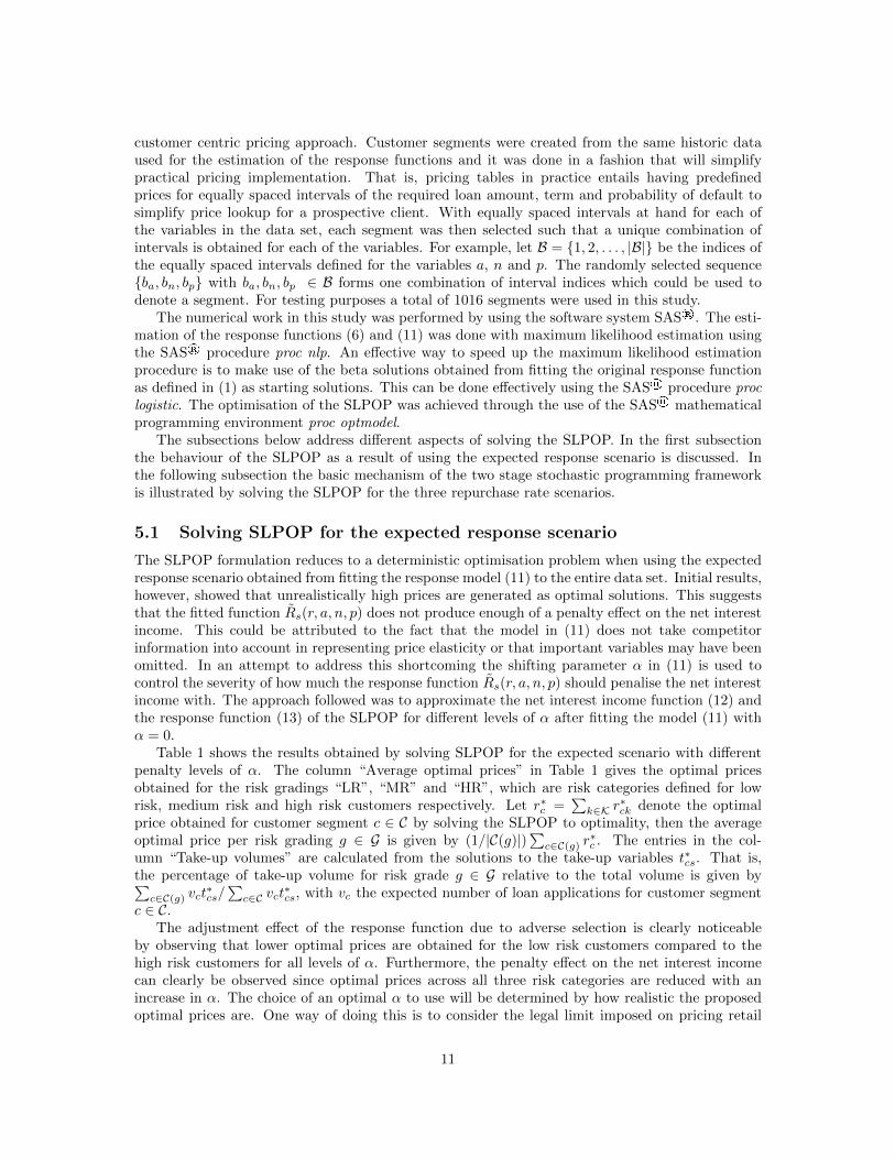
5.1 Solving SLPOP for the expected response scenario

The SLPOP formulation reduces to a deterministic optimisation problem when using the expectedresponse scenario obtained from fitting the response model (11) to the entire data set. Initial results,however, showed that unrealistically high prices are generated as optimal solutions. This suggeststhat the fitted function Rs(r, a, n, p) does not produce enough of a penalty effect on the net interestincome. This could be attributed to the fact that the model in (11) does not take competitorinformation into account in representing price elasticity or that important variables may have beenomitted. In an attempt to address this shortcoming the shifting parameter α in (11) is used tocontrol the severity of how much the response function Rs(r, a, n, p) should penalise the net interestincome with. The approach followed was to approximate the net interest income function (12) andthe response function (13) of the SLPOP for different levels of α after fitting the model (11) withα = 0.

Table 1 shows the results obtained by solving SLPOP for the expected scenario with differentpenalty levels of α. The column “Average optimal prices” in Table 1 gives the optimal pricesobtained for the risk gradings “LR”, “MR” and “HR”, which are risk categories defined for lowrisk, medium risk and high risk customers respectively. Let r∗c =

∑k∈K r

∗ck denote the optimal

price obtained for customer segment c ∈ C by solving the SLPOP to optimality, then the averageoptimal price per risk grading g ∈ G is given by (1/|C(g)|)

∑c∈C(g) r

∗c . The entries in the col-

umn “Take-up volumes” are calculated from the solutions to the take-up variables t∗cs. That is,the percentage of take-up volume for risk grade g ∈ G relative to the total volume is given by∑c∈C(g) vct

∗cs/∑c∈C vct

∗cs, with vc the expected number of loan applications for customer segment

c ∈ C.The adjustment effect of the response function due to adverse selection is clearly noticeable

by observing that lower optimal prices are obtained for the low risk customers compared to thehigh risk customers for all levels of α. Furthermore, the penalty effect on the net interest incomecan clearly be observed since optimal prices across all three risk categories are reduced with anincrease in α. The choice of an optimal α to use will be determined by how realistic the proposedoptimal prices are. One way of doing this is to consider the legal limit imposed on pricing retail

11

LR MR HR LR MR HR

0.00 59.7% 64.4% 67.5% 30.7% 27.1% 42.2%

0.50 53.1% 57.0% 60.5% 30.7% 26.9% 42.4%

1.00 46.3% 50.0% 53.5% 31.0% 26.9% 42.0%

1.50 39.4% 42.8% 46.5% 30.7% 26.8% 42.4%

2.00 33.0% 35.8% 39.3% 31.0% 26.4% 42.6%

2.50 25.7% 28.6% 32.3% 31.0% 27.0% 42.0%

2.75 22.7% 25.0% 28.8% 31.0% 26.5% 42.6%

Penalty

level ( )

Take up volumesAverage optimal prices

Table 1: Optimisation results showing the effect of the penalty level α on the SLPOP for the expectedresponse scenario.

loans. Within the South African context the legal limit is given by the formula 2.2r0 + 0.2 withr0 the repurchase rate. Considering that at the time of this study the repurchase rate was at 5%,the maximum allowable price legally is 31%. Therefore, the optimal α that will be used in theremainder of this paper will be α = 2.75 since the optimal prices obtained are below the legal limitover all three risk categories. Limiting the prices could also be achieved by imposing an upper limiton the price variables rc. However, the suggested penalty approach aims at controlling the severityof the response function while maintaining its functional form across different risk categories anddifferent customer segments. This will not be achieved by only imposing an upper limit on thepricing variables.

5.2 Solving SLPOP for the repurchase rate scenarios

In order to show the benefit of using a stochastic programming framework evidence must be providedthat show an improvement in net present income by solving the SLPOP with different scenarioscompared to solving the SLPOP using only the expected scenario (which reduces the SLPOP to asimple deterministic optimisation problem). To achieve this a test was performed by which optimalprices rESc , for each customer segment c ∈ C, are obtained by solving the SLPOP with the expectedscenario (ES) and by re-calculating the following objective function using the three repurchase ratescenarios: ∑

c∈C

∑s∈S

I(rESc , ac, nc, vc, pc, δ)Rs(rESc , ac, nc, pc) (17)

This was done to see if it would be reasonable to use the “expected” optimal prices in calculatingthe net present interest income for different realisations of future response scenarios. A desirableoutcome, therefore, would be if the objective function value obtained by solving SLPOP over allthree repurchase rate scenarios simultaneously, given by (18) below, is greater than the objectivefunction value provided by (17):∑

c∈C

∑s∈S

I(rRSSc , ac, nc, vc, pc, δ)Rs(rRSSc , ac, nc, pc) (18)

where rRRSc are the optimal prices obtained by solving the SLPOP over all three repurchase ratescenarios (RRS) simultaneously. For subsequent empirical results the use of SLPOP requires thescenario probabilities ρs, for each scenario s ∈ S. Table 2 provides three cases that relate to differentrepurchase rate scenarios and the associated scenario probabilities. For the first case we assumethat the current repurchase rate is high and a meaningful future outcome is that the repurchase

12

(1) Decrease (2) Constant (3) Increase

Decreasing 60.0% 20.0% 20.0%

Constant 20.0% 60.0% 20.0%

Increasing 20.0% 20.0% 60.0%

Future

repurchase

rate scenarios

Scenario probabilities

Table 2: Input cases based on different repurchase rate levels and future scenarios.

LR MR HR LR MR HR

1 (decrease) 60% 24.6% 24.1% 51.3%

2 (constant) 20% 40.0% 31.1% 28.9%

3 (increase) 20% 9.0% 11.9% 79.1%

1 (decrease) 60% 26.3% 27.8% 45.9%

2 (constant) 20% 41.3% 37.1% 21.6%

3 (increase) 20% 20.2% 29.8% 50.0%

Realised take up volumesData set

Average optimal prices Repurchase

rate scenarios

Scenario

probability

Objective

improvement

Repurchase rate

scenarios17.9% 21.1% 25.9% 6.4%

Repurchase rate

scenarios

vol(HR) <= 50

16.8% 19.5% 26.4% 5.3%

Table 3: Optimisation results for the case with an expected decrease in repurchase rate.

rate will most likely decrease. For this case the probabilities of 60%, 20% and 20% are assigned toa decreasing, a constant and an increasing repurchase rate scenario respectively. For the case wherethe current repurchase rate is on an average historic level the probabilities of 20%, 60% and 20%are assigned to a decreasing, a constant and an increase repurchase rate scenario respectively, toindicate that we expect the repurchase rate to remain unchanged. For the final case a low currentrepurchase rate is assumed with the future expectation that it will increase, making it reasonableto assign the probabilities of 20%, 20% and 60% to a decreasing, a constant and an increasingrepurchase rate scenario respectively.

Table 3 shows the optimisation results for the first case were we consider a high current repur-chase rate with a high probability that it may decrease in future. The first row provides the averageoptimal prices for the low risk “LR”, medium risk “MR” and high risk “HR” categories respectivelywhen solving SLPOP using all three repurchase rate scenarios simultaneously. For the same rowthe value in the column “Objective improvement” gives the percentage improvement obtained insolving the SLPOP with all three repurchase rate scenarios, compared to solving the SLPOP usingonly the expected scenario. That is, the percentage improvement is obtained by calculating thethe relative improvement of (18) over (17). The improvement of 6.4% in net present interest in-come shows that the optimal prices obtained by solving the SLPOP over the three repurchase ratescenarios simultaneously are more robust compared to the “expected” optimal prices. By solvingthe SLPOP over all available scenarios simultaneously more information is taken into account andoptimal prices are better balanced against the effect of scenario dependent take-up volumes thatinfluence the objective function value. Continuing with the analysis of the second row of Table 3 weobserve that the take-up volumes for the “HR” category for the first scenario represents about 50%of the total volume. For the third scenario, however, the proportion of high risk volume is almost

13

LR MR HR LR MR HR

1 (decrease) 20% 24.2% 23.6% 52.1%

2 (constant) 60% 38.2% 29.6% 32.2%

3 (increase) 20% 9.9% 11.5% 78.6%

1 (decrease) 20% 26.2% 27.8% 46.0%

2 (constant) 60% 40.4% 36.6% 23.0%

3 (increase) 20% 20.4% 29.6% 50.0%

Realised take up volumesData set

Average optimal prices Repurchase

rate scenarios

Scenario

probability

Objective

improvement

Repurchase rate

scenarios17.3% 20.0% 24.0% 10.6%

Repurchase rate

scenarios

vol(HR) <= 50

15.8% 17.7% 25.1% 8.9%

Table 4: Optimisation results for the case with the expectation that repurchase rate will remain unchanged.

LR MR HR LR MR HR

1 (decrease) 20% 25.4% 24.2% 50.5%

2 (constant) 20% 39.6% 30.4% 30.0%

3 (increase) 60% 16.1% 15.3% 68.7%

1 (decrease) 20% 26.7% 27.3% 46.0%

2 (constant) 20% 40.1% 35.6% 23.5%

3 (increase) 60% 22.3% 27.7% 50.0%

Realised take up volumesData set

Average optimal prices Repurchase

rate scenarios

Scenario

probability

Objective

improvement

Repurchase rate

scenarios16.1% 19.6% 24.9% 20.9%

Repurchase rate

scenarios

vol(HR) <= 50

14.6% 18.2% 25.6% 20.2%

Table 5: Optimisation results for the case with an expected increase in repurchase rate.

80% making it a very risky portfolio. It could be argued that since there is only a 20% probabilityof the third scenario realising in future that it may be acceptable. The SLPOP, however, doesprovide the capability to manage the portfolio risk by using the volume constraint sets (15) and(16). The second row of Table 3 gives the results for solving SLPOP using all three repurchase ratescenarios simultaneously, but with the constraint (16) imposing an upper limit of 50% on the highrisk category volume. From the results it is clear that a price is paid in terms of the net interestincome with the objective improvement now only at 5.3%. The benefit achieved however is animproved risk profile with the high risk category volume now limited to 50% for all three potentialfuture scenarios.

Table 4 shows the optimisation results for the second case were we consider an average repurchaserate (compared historically) with a high probability that it will remain unchanged in future. Onceagain an improvement in objective function value is observed when solving the SLPOP over thethree repurchase rate scenarios simultaneously. The first row shows an improvement of 10.6% butagain with a risky portfolio if scenario three happen to realise in future. The second row of Table 4shows the results for resolving SLPOP with the 50% limit on high risk volume with an improvementof 8.9% in net interest income obtained over solving the SLPOP with the expected scenario. Itshould be noted that, not only do we achieve an improvement in net interest income by solving theSLPOP over all three repurchase rate scenarios simultaneously, we are guaranteed that the scenariodependent take-up volumes adheres to the volume constraint, which is not necessarily the case forsolving the SLPOP using the expected scenario.

14

Table 5 shows the optimisation results for the thrid case were we consider a low current repur-chase rate with a high probability that there will be an increase in repurchase rate in the future.The improvements obtained in solving the SLPOP over the three repurchase rate scenarios simul-taneously without and with the volume constraint are 20.9% and 20.2% respectively. These resultsshow that meaningful results can be obtained for the credit price optimisation problem by consider-ing hypothetical scenarios like we did with the inclusion of scenario three that represents a potentialincrease in repurchase rate, a situation that is not captured in the historical data available.

6 Summary and conclusion

The price optimisation problem addressed in this paper deals with determining the optimal pricesto quote prospective customers while considering uncertainty in future price sensitivity. Thatis, the take-up rates of future loans may deviate from current levels necessitating the use of astochastic programming approach. This study is, to the best of our knowledge, a first attemptto incorporate uncertainty in price sensitivity as part of an explicitly formulated mathematicalprogramming problem.

In this study a concave response function is suggested that allows for the formulation of a lin-earised price optimisation problem that can be solved to optimality using standard linear program-ming technology. With a linear representation more complex formulations of the price optimisationproblem can be handled such as volume constraints expressed in terms of the response function.The suggested response model also ensures a finite support for the pricing decision variable whichmakes it much more realistic compared to using a logit based response function with asymptoticproperties.

The benefit of employing a stochastic programming approach was illustrated by means of em-pirical tests based on real data. Although some theoretical contributions have been made recentlytowards developing price optimisation models for retail credit, little evidence exist in literature ofempirical work supporting the benefits of employing price opitmisation technology. The results inthis study showed that by only using “expected” optimal prices either a loss in revenue can occurdue to lost opportunity, or a violation of strategic constraints can be expected when certain take-upscenarios realise in future.

7 Acknowledgement

This work is based on the research supported in part by the National Research Foundation of SouthAfrica reference number (UID: TP1207243988 ). The Grantholder acknowledges that opinions,findings and conclusions or recommendations expressed in any publication generated by the NRFsupported research are that of the authors, and that the NRF accepts no liability whatsoever inthis regard. The authors would like to extend their gratitute to Mr. Hung Chen and Mr. GordonTurnbull from Absa Bank for their inputs and effort in providing the data. The authors would alsolike to acknowledge the assistance of Prof. Hennie Venter and other staff members of the Centrefor Business Mathematics and Informatics, North-West University.

References

V. Agrawal and M. Ferguson, 2007. Bid-response models for customised pricing, Journal ofRevenue and Pricing Management 6(3), 212–228

L. Ausubel, 1999. Adverse selection in the credit card market, Working paper, University ofMaryland, available at http://www.ausubel.com/creditcard-papers/adverse.pdf

15

S. Boyd and L. Vandenberghe, 2004. Convex Optimization. Cambridge University Press, Cam-bridge.

S. Caufield, 2012. Consumer Credit Pricing. In Ozer, O. and Phillips, R. Editors, Oxford Handbookof Pricing Management. Oxford University Press, Oxford.

R.G. Cross and A. Dixit, 2005. Customer-centric pricing: The surprising secret for profitability,Business Horizons 48(6), 483–491

L. Einav, M. Jenkins and J. Levin, 2012. Contract pricing in consumer credit markets, Journalof the Econometric Society 80(4), 1387–1432

W. Edelberg, 2006. Risk-based pricing of interest rates for consumer loans, Journal of MonetaryEconomics 53, 2283–2298

J.L. Higle, 2005. Stochastic programming: Optimization when uncertainty matters, In Tutorialsin Operations Research: Emerging Theory, Methods, and Applications, INFORMS, Hanover.

B. Huang and L.C. Thomas, 2009. Credit card pricing and the impact of adverse selec-tion, Working paper, Centre for Risk Research, University of Southampton, available athttp://www.business-school.ed.ac.uk/crc/conferences/conference-archive?a=45866

D.S. Karlan and J. Zinman, 2008. Credit elasticities in less-developed economies: implicationsfor microfinance, American Economic Review 98(3), 1040–1068

B.V. Oliver and R.M. Oliver, 2012. Optimal ROE loan pricing with or without ad-verse selection, Journal of the Operational Research Society, Advance Online Publication,doi:10.1057/jors2012.87

S. Park, 1997. Effects of price competition in the credit card industry, Economics Letters 57(1),79–85

R.L. Phillips, 2005. Pricing and revenue optimization. Stanford University Press, Stanford, CA.

R.L. Phillips and R. Raffard, 2009. Theory and empirical evidence for price-driven adverseselection in consumer lending, In Proceedings of Credit Scoring Conference - XI, Edinburgh, UK

R.L. Phillips, 2012. Customized pricing. In Ozer, O. and Phillips, R. Editors, Oxford Handbookof Pricing Management. Oxford University Press, Oxford.

R.L. Phillips, 2013. Optimizing prices for consumer credit, Working paper No. 2013-1, ColumbiaUniversity, available at http://www7.gsb.columbia.edu/cprm/sites/default/files/files/2013-1 Price Opt for Cons Credit.pdf

G. Skugge, 2011. The future of pricing: Outside-in, Journal of Revenue and Pricing Management10(4), 392–395

J. Stiglitz and A. Weiss, 1981. Credit rationing in markets with imperfect information, Amer-ican Economic Review 71(3), 393–410

L.C. Thomas, 2009. Consumer credit models: pricing, profit and portfolios. Oxford UniversityPress, Oxford.

16