creative inquiry electronics project lab manual inquiry electronics project lab manual ni mydaq

1

Creative Inquiry Electronics Project

Lab Manual

NI myDAQ

®

®

2

TABLE OF CONTENTS

Introduction ............................................................................................................................... 5

LabVIEW Package and Driver Installation Tutorial for ENGR 190.......................... 5

Basic Troubleshooting ............................................................................................................ 6

Files on ENGR190_VIs.zip ....................................................................................................... 7

Lab 01: myDAQ, LabVIEW®, and MySnapTM ..................................................................... 8 1.1 Overview ........................................................................................................... 8 1.2 Topics covered in Lab 01 .................................................................................. 8 1.3 Objective: .......................................................................................................... 8 1.4 What You Need: ................................................................................................ 8 1.5 Instructions: ....................................................................................................... 9 1.6 Resistors ......................................................................................................... 11 1.7 Insulators ........................................................................................................ 12 1.8 Review ............................................................................................................ 12 1.9 MyDAQ® and LabVIEW®: ................................................................................ 12 1.10 Building the Front Panel: ................................................................................. 13 1.11 Coding Strategy: ............................................................................................. 17 1.12 How It Works: .................................................................................................. 19 1.13 Storing Data: ................................................................................................... 19 1.14 Tips and Tricks: ............................................................................................... 20

Lab 02 (Part I): Multisim & Resistors in Series ........................................................... 21 2.1 Topics covered in Lab 02 (Part I) .................................................................... 21 2.2 Objective: ........................................................................................................ 21 2.3 What You Need: .............................................................................................. 21 2.4 Multisim & Circuit Emulation ............................................................................ 22 2.5 NI myDAQ and Real World ............................................................................. 23 2.6 LabVIEW® ....................................................................................................... 24 2.7 How It Works: .................................................................................................. 25

Lab 02 (Part II): Multisim and Resistors in Parallel .................................................. 26 2.8 Topics covered in Lab 02 (Part II) ................................................................... 26 2.9 Objective: ........................................................................................................ 26 2.10 Multisim & Circuit Emulation ............................................................................ 26 2.11 MyDAQ & Real World ..................................................................................... 27 2.12 LabVIEW®: ...................................................................................................... 28 2.13 Review ............................................................................................................ 29

Lab 03: Voltage Generators and Viewers ...................................................................... 30 3.1 Topics covered in Lab 03 ................................................................................ 30 3.2 Objective: ........................................................................................................ 30 3.3 What You Need: .............................................................................................. 30 3.4 Definitions ....................................................................................................... 30 3.5 Water Pipe Analogy ........................................................................................ 31 3.6 Building in the Lab: AC and DC Voltage Sources ............................................ 33 3.7 Summary ........................................................................................................ 36

Lab 04: Ohms Law .................................................................................................................. 37 4.1 Topics covered in Lab 04 ................................................................................ 37 4.2 Objective: ........................................................................................................ 37 4.3 What You Need: .............................................................................................. 37 4.4 Ohms Law: ...................................................................................................... 38 4.5 Multisim: Virtual World .................................................................................... 38 4.6 MySnapTM: Real World .................................................................................. 40

3

4.7 Hardware Limits .............................................................................................. 41 4.8 Summary: ....................................................................................................... 43 4.9 Know Your Equipment Review: ....................................................................... 43

Lab 05: Kirchhoff's Voltage Law ....................................................................................... 44 5.1 Topic covered in Lab 05 .................................................................................. 44 5.2 Objective: ........................................................................................................ 44 5.3 What You Need: .............................................................................................. 44 5.4 The Circuit:...................................................................................................... 45 5.5 Multisim Verification of Kirchhoff’s Voltage Law (KVL): ................................... 45 5.6 MyDAQ DMM Measurements.......................................................................... 45 5.7 Sources for Error ............................................................................................. 46

Lab 06: Capacitors ................................................................................................................. 47 6.1 Topics covered in Lab 06 ................................................................................ 47 6.2 Objective: ........................................................................................................ 47 6.3 What You Need: .............................................................................................. 48 6.4 Water Pipe Analogy: ....................................................................................... 48 6.5 Understanding Capacitor Properties:............................................................... 49 6.6 Multisim Capacitor Circuit: ............................................................................... 50 6.7 More About Capacitor Properties: ................................................................... 51 6.8 Transient Responses: ..................................................................................... 52 6.9 RC time constant:............................................................................................ 53 6.10 The Real World - MySnapTM: ........................................................................... 54 6.11 Actual Values and Tolerances: ........................................................................ 55 6.12 LabVIEW® RC Meter: ...................................................................................... 56 6.13 How it Works: .................................................................................................. 57 6.14 Review: ........................................................................................................... 57

Lab 07: Inductors ................................................................................................................... 59 7.1 Topics covered in Lab 07 ................................................................................ 59 7.2 Objective: ........................................................................................................ 59 7.3 What You Need: .............................................................................................. 60 7.4 Water Pipe Analogy: ....................................................................................... 60 7.5 In electric circuits: ............................................................................................ 61 7.6 Multisim Inductor Circuit: ................................................................................. 62 7.7 More About Inductor Properties: ...................................................................... 62 7.8 Transient Responses: ..................................................................................... 63 7.9 RL time constant: ............................................................................................ 64 7.10 The Real World - MySnapTM: ........................................................................... 64 7.11 Actual Values and Tolerances: ........................................................................ 66 7.12 LabVIEW® LCR Meter: .................................................................................... 66 7.13 How it Works: .................................................................................................. 68 7.14 Review: ........................................................................................................... 68

Lab 08: The Diode .................................................................................................................. 70 8.1 Topics covered in Lab 08 ................................................................................ 70 8.2 Objective: ........................................................................................................ 70 8.3 What You Need: .............................................................................................. 71 8.4 Water Pipe Analogy: ....................................................................................... 71 8.5 In Electronic Circuits: ...................................................................................... 72 8.6 Multisim Diode Circuit: .................................................................................... 73 8.7 AC to DC Conversion: ..................................................................................... 73 8.8 More About Diode Properties: ......................................................................... 73 8.9 The Real World Diode: .................................................................................... 74 8.10 Diode (D1) Measured Parameters ................................................................... 76 8.11 Diode Equation ............................................................................................... 77

4

8.12 Review: ........................................................................................................... 78

Appendix A: Basic Definitions and Conventions ......................................................... 79

Appendix B: Multisim Setup ............................................................................................. 83

Appendix C: Building Snap-Circuits ® ........................................................................... 84

Appendix D: Worksheets .................................................................................................... 85

5

Introduction

This document is based on the “Learn-by-Doing”® principle because simply

reading about a technical subject is not the best way to learn. After all, you don't

read about putting together a jigsaw puzzle, you put the puzzle together to solve

the picture! Reading about a maze may help you to move through but doing the

maze gives you the course you must take to get through it. Engineering is the

same way. You must actually build circuits and programs in order to really

understand the concepts.

The topics are covered in a straightforward, simplified manner which

allows you to quickly understand the fundamental principles. After the main topic

of each chapter is introduced, sub-topics are explored in a step by step manner

with explanations given for each new engineering principle. Each chapter

contains single topic-usually. First, you read about the topic and then you see

examples that let you work in the virtual world to understand how the concepts

can be applied to actual circuits. You then work in the real world with real

electronic components to see how they differ from the mathematical models and

what their limitations might do to an engineered design.

Each section finishes with a review of what was covered in the material in

that section. The principles usually come from the text or are deducible from the

text, but occasionally you might need to experiment a little to really understand

how to use them. After completing each section you'll begin to understand more

of the concepts and realizing that now you know the answers can be a big

confidence builder.

LabVIEW Package and Driver Installation Tutorial

It is important that student should install all the required software for the course

before continuing to next section. A tutorial is provided on course webpage for

step by step installation of the LabVIEW, NI Multisim and MyDAQ drivers.

6

Basic Troubleshooting

1. Most circuit problems are due to incorrect assembly, always double check

that your circuit exactly matches the drawing for it.

2. Be sure that parts with positive or negative markings are positioned as

shown in the drawings.

3. Be sure that all connections are securely fastened.

4. Always use a power switch to remove power when building circuits.

5. Always check circuits before turning on power.

6. Use myDAQ digital multi-meter (DMM) to test MySnap components if they

appear to be damaged or not working properly.

7. Use eye protection when experimenting on your own circuits.

8. Always remove power if circuit does not perform properly, and then use

myDAQ DMM to check circuit for shorts or opens.

WARNING: SHOCK HAZARD

Never connect any component or lead to electrical outlets in any way

WARNING: EXTERNAL POWER SOURCES

Use external power sources or batteries at your own risk as they may cause

damage to components or Computer USB ports.

!

7

Files on ENGR190_VIs.zip

The ENGR190_Vis.zip file is available to students on following course webpage.

www.clemson.edu/ces/departments/ece/undergrad/ElectronicsProject.html

Students should download above file and unzip in on his/her computer. The Zip

file contains LabVIEW VIs and other files which will be used in some of the

experiments during the course.

Resistors.pdf - Description of how resistors are manufactured and

constructed.

Cap.gif - Water pipe analogy of a Capacitor.

Coil.gif - Water pipe analogy of an Inductor.

Diode.gif - Water pipe analogy of a diode.

RinParallel.gif - Water pipe analogy of two resistors in parallel.

VI’s on zip file: C_Meter.vi, Diode.vi, LCR_Meter.vi, PartsTest1.vi, R_Graph.vi,

RinSeries.vi, Karaoke myDAQ.vi

8

Lab 01: myDAQ, LabVIEW®, and MySnapTM

1.1 Overview

This section explores using a National Instruments myDAQ to measure the

resistance Conductors, Insulators, and Resistors. The measurements will be

taken with the myDAQ DMM (Digital Multi-Meter). The components needed are

supplied in the MySnap™ kit for myDAQ. Real life applications apply to any

occupation that uses electrical components or devices.

1.2 Topics covered in Lab 01

Objective

What You Need

Instructions

Resistors

Insulators

Review

myDAQ and LabVIEW®

Building the Front Panel

Coding Strategy

How It Works

Storing Data

Tips and Tricks

1.3 Objective:

Use the DMM terminals on the NI myDAQ and LabVIEW to measure and record

the DC resistance of various conductors, resistors, and insulators supplied in the

MySnapTM kit.

1.4 What You Need:

NI myDAQ

Computer with LabVIEW and NI ELVISmx installed

MySnap™ kit

9

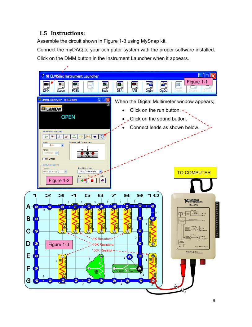
1.5 Instructions:

Assemble the circuit shown in Figure 1-3 using MySnap kit.

Connect the myDAQ to your computer system with the proper software installed.

Click on the DMM button in the Instrument Launcher when it appears.

When the Digital Multimeter window appears;

Click on the run button.

Click on the sound button.

Connect leads as shown below.

CONDUCTORS

Figure 1-1

Figure 1-2

TO COMPUTER

Figure 1-3

1

1 1 1 1 1 1 1

1

1

1

1

2

2 2

1

2 3 3 3

3

2

2 3 3

2

4

2

1K Resistors

10K Resistors

100K Resistor

10

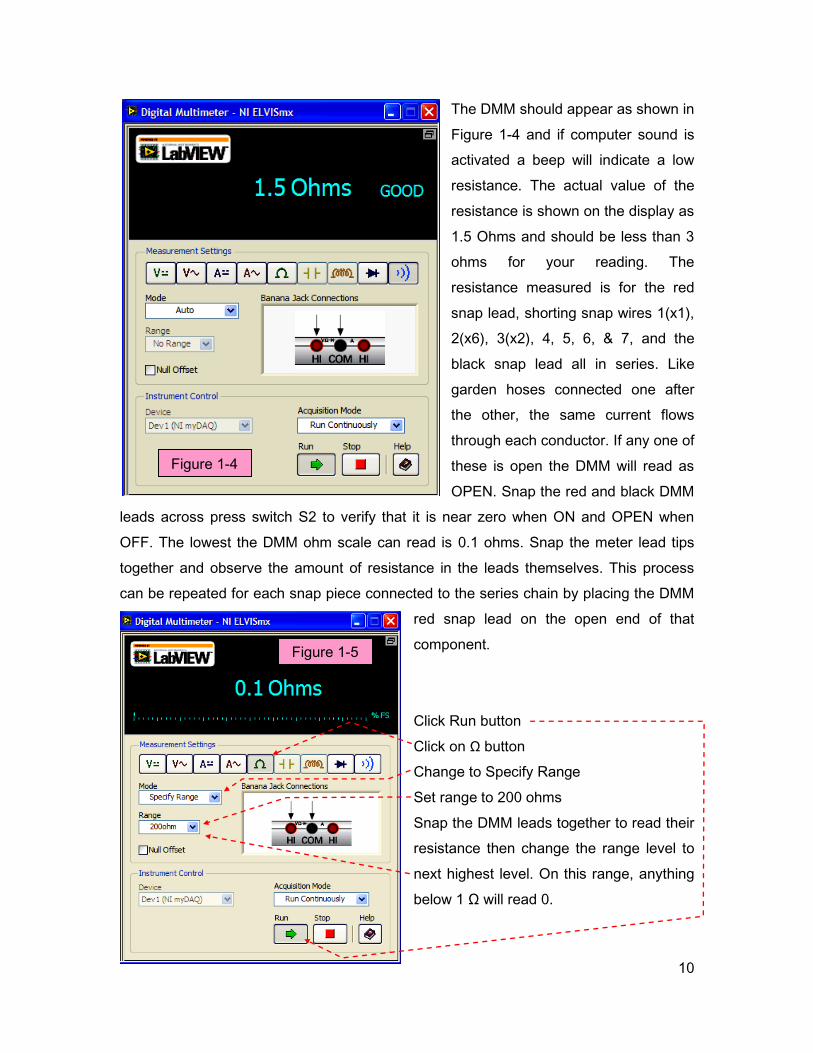
The DMM should appear as shown in

Figure 1-4 and if computer sound is

activated a beep will indicate a low

resistance. The actual value of the

resistance is shown on the display as

1.5 Ohms and should be less than 3

ohms for your reading. The

resistance measured is for the red

snap lead, shorting snap wires 1(x1),

2(x6), 3(x2), 4, 5, 6, & 7, and the

black snap lead all in series. Like

garden hoses connected one after

the other, the same current flows

through each conductor. If any one of

these is open the DMM will read as

OPEN. Snap the red and black DMM

leads across press switch S2 to verify that it is near zero when ON and OPEN when

OFF. The lowest the DMM ohm scale can read is 0.1 ohms. Snap the meter lead tips

together and observe the amount of resistance in the leads themselves. This process

can be repeated for each snap piece connected to the series chain by placing the DMM

red snap lead on the open end of that

component.

Click Run button

Click on Ω button

Change to Specify Range

Set range to 200 ohms

Snap the DMM leads together to read their

resistance then change the range level to

next highest level. On this range, anything

below 1 Ω will read 0.

Figure 1-4

Figure 1-5

11

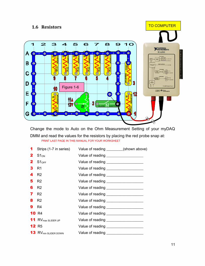
1.6 Resistors

Change the mode to Auto on the Ohm Measurement Setting of your myDAQ

DMM and read the values for the resistors by placing the red probe snap at:

1 Strips (1-7 in series) Value of reading _________(shown above)

2 S1ON Value of reading ____________________

2 S1OFF Value of reading ____________________

3 R1 Value of reading ____________________








11 RVmax SLIDER UP Value of reading ____________________


13 RVmin SLIDER DOWN Value of reading ____________________

Figure 1-5

TO COMPUTER

Figure 1-6

PRINT LAST PAGE IN THIS MANUAL FOR YOUR WORKSHEET

12

1.7 Insulators

Using the DMM pointed probes try measuring the resistance of the myDAQ case,

the MySnapTM base grid, or the outside of the wire on the jumper leads. Take

care when measuring wire insulation and do not push points into the insulation.

Use the flat side of the probe tips.

1.8 Review Conventional electric current moves from the positive surplus side of the

battery (+) to the deficiency side of the battery (-)

Conductors allow electrical current to easily flow because of their free

electrons.

Resistors allow current to flow to some degree in proportion to their

resistance in ohms.

Insulators oppose electrical current.

The MySnapTM system includes components that can be classified as

conductors, resistors, or insulators.

The myDAQ DMM can be used to determine the class of a component

and can measure the value of resistance in most components that are not

insulators or good conductors.

1.9 MyDAQ® and LabVIEW®:

LabVIEW® was designed to quickly check and record electronic data. In this

section you will use LabVIEW® to measure and record the resistance values of

the components you measured previously. Each part will be measured and data

recorded in a similar fashion to the testing performed when these components

were manufactured. The numeric indicator will display the instantaneous value

and the table will store the data when the record button is clicked. The values will

be graphed for a quick visual display of all the values.

Open LabVIEW program that has been installed on your computer. When the

getting started screen appears, pick the Blank VI option to build the program that

will be used to check your MySnapTM parts. Your process will be as follows;

1.) Build the front panel screen.

2.) Open the programming window and build program to drive front panel.

3.) Measure, Display, and Store resistive data about each part.

13

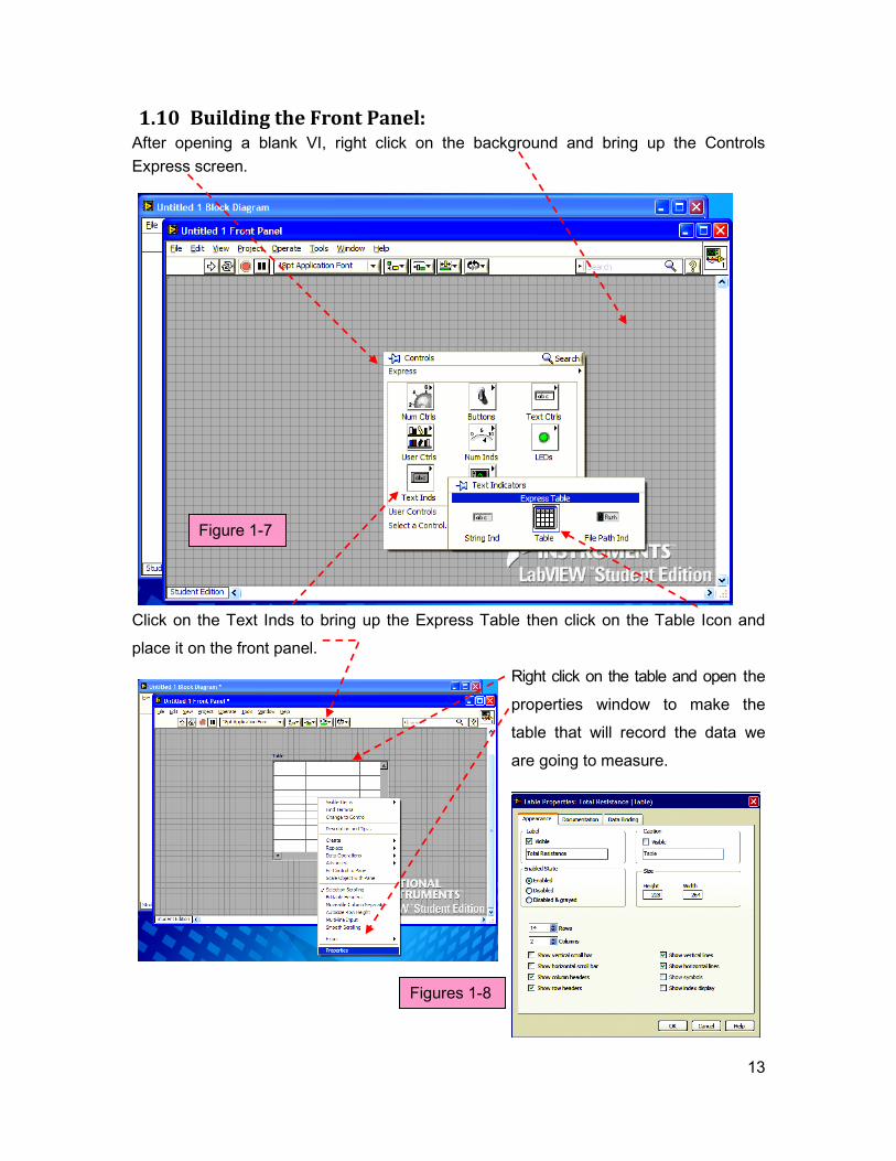
1.10 Building the Front Panel: After opening a blank VI, right click on the background and bring up the Controls

Express screen.

Click on the Text Inds to bring up the Express Table then click on the Table Icon and

place it on the front panel.

Right click on the table and open the

properties window to make the

table that will record the data we

are going to measure.

Figure 1-7

Figures 1-8

14

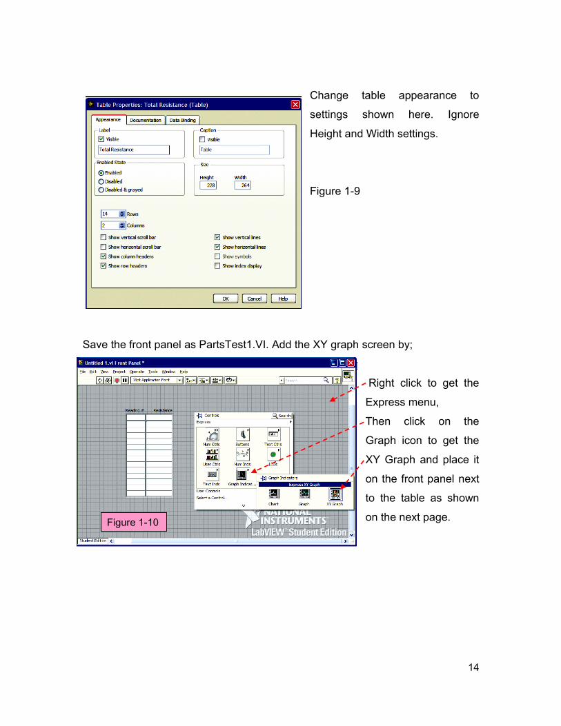
Change table appearance to

settings shown here. Ignore

Height and Width settings.

Figure 1-9

Save the front panel as PartsTest1.VI. Add the XY graph screen by;

Right click to get the

Express menu,

Then click on the

Graph icon to get the

XY Graph and place it

on the front panel next

to the table as shown

on the next page.

Figure 1-9

Figure 1-10

15

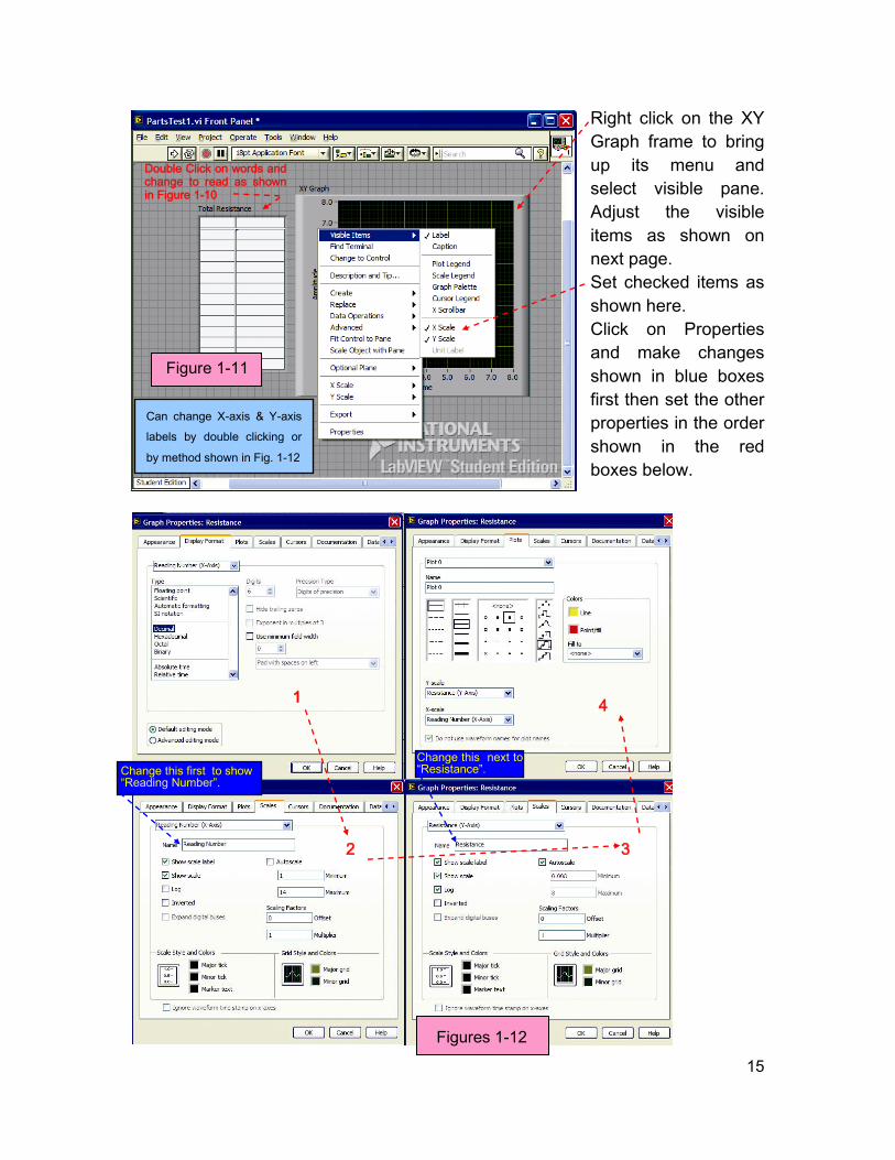
Right click on the XY

Graph frame to bring

up its menu and

select visible pane.

Adjust the visible

items as shown on

next page.

Set checked items as

shown here.

Click on Properties

and make changes

shown in blue boxes

first then set the other

properties in the order

shown in the red

boxes below.

Figure 1-11

Double Click on words and change to read as shown in Figure 1-10

1

2 3

4

Figures 1-12

Change this first to show “Reading Number”.

Change this next to “Resistance”.

Can change X-axis & Y-axis

labels by double clicking or

by method shown in Fig. 1-12

16

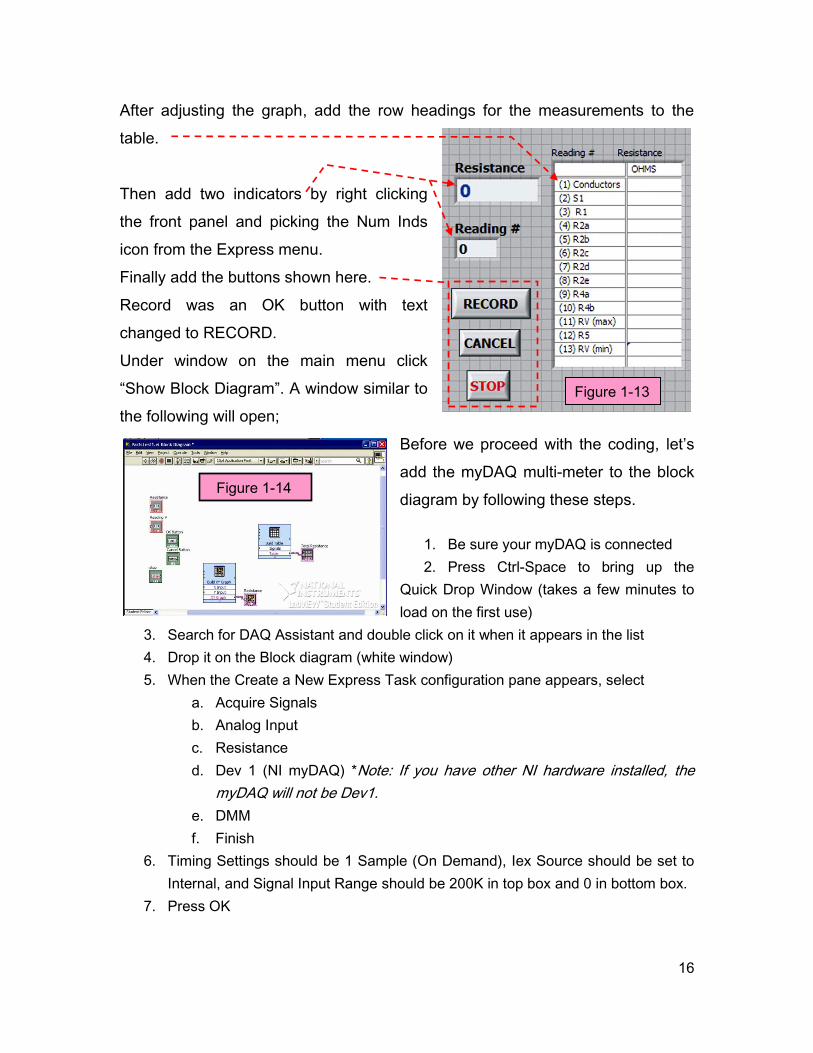
After adjusting the graph, add the row headings for the measurements to the

table.

Then add two indicators by right clicking

the front panel and picking the Num Inds

icon from the Express menu.

Finally add the buttons shown here.

Record was an OK button with text

changed to RECORD.

Under window on the main menu click

“Show Block Diagram”. A window similar to

the following will open;

Before we proceed with the coding, let’s

add the myDAQ multi-meter to the block

diagram by following these steps.

1. Be sure your myDAQ is connected

2. Press Ctrl-Space to bring up the

Quick Drop Window (takes a few minutes to

load on the first use)

3. Search for DAQ Assistant and double click on it when it appears in the list

4. Drop it on the Block diagram (white window)

5. When the Create a New Express Task configuration pane appears, select

a. Acquire Signals

b. Analog Input

c. Resistance

d. Dev 1 (NI myDAQ) *Note: If you have other NI hardware installed, the

myDAQ will not be Dev1.

e. DMM

f. Finish

6. Timing Settings should be 1 Sample (On Demand), Iex Source should be set to

Internal, and Signal Input Range should be 200K in top box and 0 in bottom box.

7. Press OK

Figures 1-13

Figure 1-13

Figure 1-14

17

1.11 Coding Strategy:

A front panel to display the resistance values in a numerical indicator, a table to

store this data, and a graph to display data has been created in LabVIEW®. We

will acquire the data using the DAQ Assistant you just placed on the block

diagram and then pass the data to the indicator. After the reading appears, we

will store the data in the table and on the graph. The reading number is then

incremented, the resistance probe is moved, and the process is repeated.

Figure 1-15: Coding Block Diagram

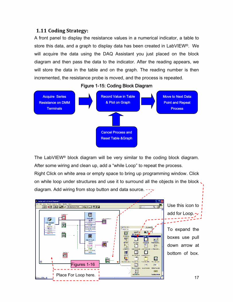
The LabVIEW® block diagram will be very similar to the coding block diagram.

After some wiring and clean up, add a “while Loop” to repeat the process.

Right Click on white area or empty space to bring up programming window. Click

on while loop under structures and use it to surround all the objects in the block

diagram. Add wiring from stop button and data source.

Use this icon to

add for Loop.

To expand the

boxes use pull

down arrow at

bottom of box.

Acquire Series

Resistance on DMM

Terminals

Record Value in Table

& Plot on Graph

Move to Next Data

Point and Repeat

Process

Cancel Process and

Reset Table &Graph

Figure 1-17

Figures 1-16

Place For Loop here.

18

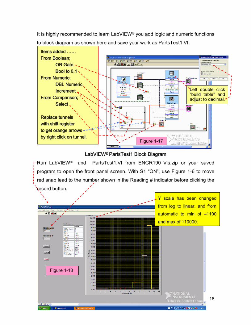
It is highly recommended to learn LabVIEW® you add logic and numeric functions

to block diagram as shown here and save your work as PartsTest1.VI.

LabVIEW® PartsTest1 Block Diagram

Run LabVIEW® and PartsTest1.VI from ENGR190_Vis.zip or your saved

program to open the front panel screen. With S1 “ON”, use Figure 1-6 to move

red snap lead to the number shown in the Reading # indicator before clicking the

record button.

Items added ……

From Boolean;

OR Gate

Bool to 0,1

From Numeric;

DBL Numeric

Increment

From Comparison;

Select

Replace tunnels

with shift register

to get orange arrows

by right click on tunnel. Figure 1-17

Y scale has been changed

from log to linear, and from

automatic to min of –1100

and max of 110000.

Left double click “build table” and adjust to decimal.

Figure 1-18

19

THE PREVIOUS VIRTUAL INSTRUMENT WAS SHOWN IN DETAIL TO HELP

THE USER UNDERSTAND THE POWER OF LABVIEW®. FUTURE VI’S WILL

BE PROVIDED WITHOUT THIS IN DEPTH DETAIL.

1.12 How It Works: Inside the while loop on the upper-left is the DAQ Assistant used to input the

resistance data from the DMM terminals. The resistance values are indicated on

the front panel in the Measurements numeric indicator labeled “Resistance”. In

this VI the DAQ Assistant is configured for on-demand input on the analog

channel. Therefore every time the red snap lead is moved, the Resistance

Indicator will be updated. After the record button is clicked, the Reading number

will increment for the next reading. The red snap in Figure 1-7 should always be

on the number label that is the same as the Reading # when the record button is

clicked.

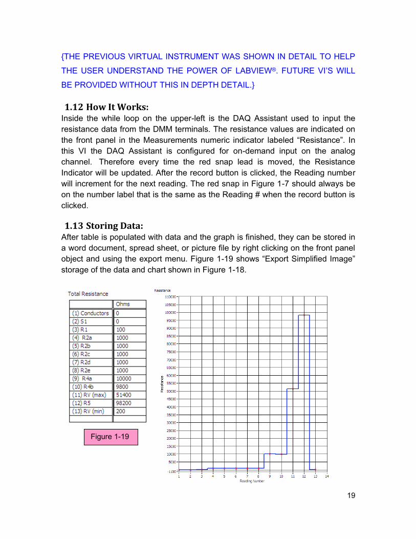
1.13 Storing Data: After table is populated with data and the graph is finished, they can be stored in

a word document, spread sheet, or picture file by right clicking on the front panel

object and using the export menu. Figure 1-19 shows “Export Simplified Image”

storage of the data and chart shown in Figure 1-18.

Figure 1-19

20

1.14 Tips and Tricks:

Run the animated gif file called RinParallel.gif that is on the MySnap™ disc for an

analogy of resistance using water pipes. The top water pipe is filled with rocks

and has low resistance, while the lower pipe is filled with sand and has high

resistance.

Review the Resistors.pdf file for more information on how resistors are

manufactured and the different types of resistors.

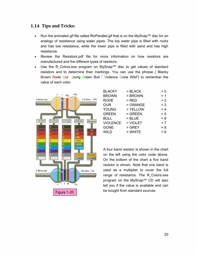
Use the R_Colors.exe program on MySnap™ disc to get values of standard

resistors and to determine their markings. You can use the phrase Blacky

Brown Rode Our Young Green Bull “ Violence Gone Wild” to remember the

value of each color.

BLACKY = BLACK = 0

BROWN = BROWN = 1

RODE = RED = 2

OUR = ORANGE = 3

YOUNG = YELLOW = 4

GREEN = GREEN = 5

BULL = BLUE = 6

VIOLENCE = VIOLET = 7

GONE = GREY = 8

WILD = WHITE = 9

A four band resistor is shown in the chart

on the left using the color code above.

On the bottom of the chart a five band

resistor is shown. Note that one band is

used as a multiplier to cover the full

range of resistance. The R_Colors.exe

program on the MySnapTM CD will also

tell you if the value is available and can

be bought from standard sources.

Figure 1-20

21

Lab 02 (Part I): Multisim & Resistors in Series

This portion explains using Multisim, myDAQ, LabVIEW® , and MySnapTM to study and

observe the effect of resistors that are connected in a manner that forces the same

current to pass through each resistor. This type of connection is called series

connection.

2.1 Topics covered in Lab 02 (Part I)

Objective

What You Need

Multisim & Circuit Emulation

MyDAQ & Real World

LabVIEW®

How it Works

2.2 Objective:

Use Multisim to emulate and study a circuit on a computer, and then use myDAQ

with LabVIEW® to measure and observe the same circuit as resistors are placed

in series on the MySnap™ base. Real life applications apply to any occupation

that uses electronic test equipment to measure resistance.

2.3 What You Need:

Multisim

NI myDAQ

LabVIEW®

MySnap™ BASIC ELECTRONICS EE100 kit

Computer System with above software installed.

22

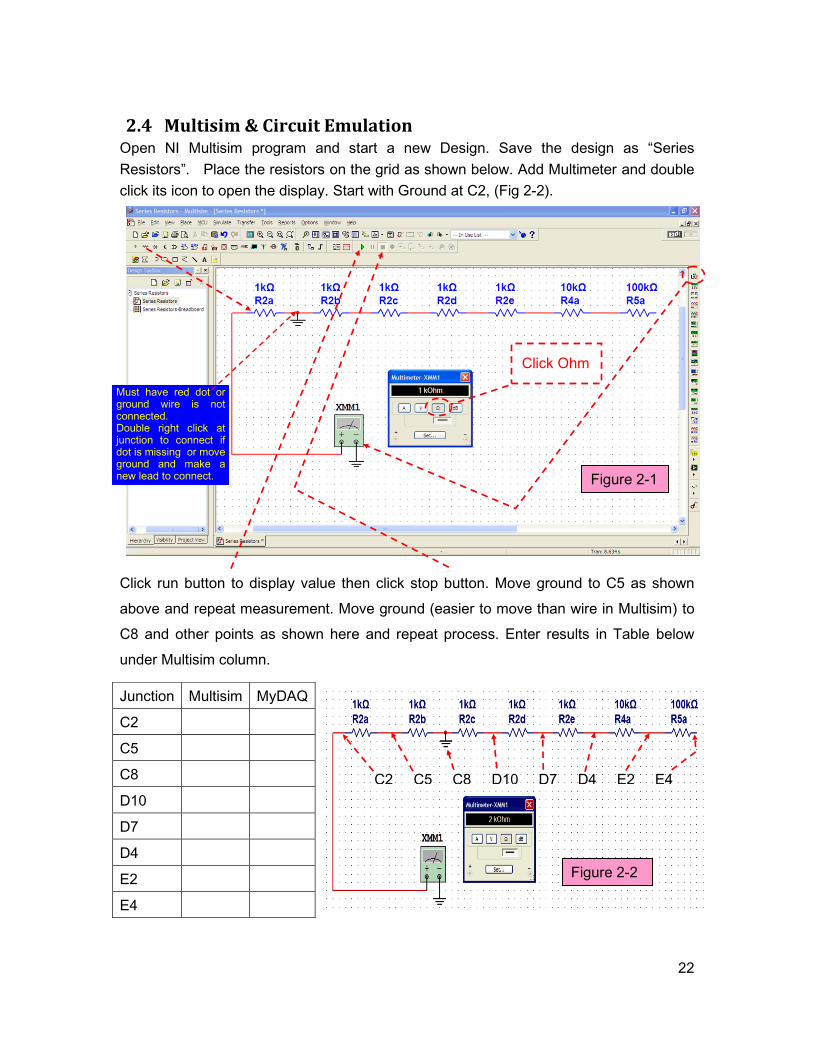
2.4 Multisim & Circuit Emulation Open NI Multisim program and start a new Design. Save the design as “Series

Resistors”. Place the resistors on the grid as shown below. Add Multimeter and double

click its icon to open the display. Start with Ground at C2, (Fig 2-2).

Click run button to display value then click stop button. Move ground to C5 as shown

above and repeat measurement. Move ground (easier to move than wire in Multisim) to

C8 and other points as shown here and repeat process. Enter results in Table below

under Multisim column.

Junction Multisim MyDAQ

C2

C5

C8

D10

D7

D4

E2

E4

Figure 2-2

C2 C5 C8 D10 D7 D4 E2 E4

Figure 2-1

Click Ohm

Must have red dot or ground wire is not connected. Double right click at junction to connect if dot is missing or move ground and make a new lead to connect.

23

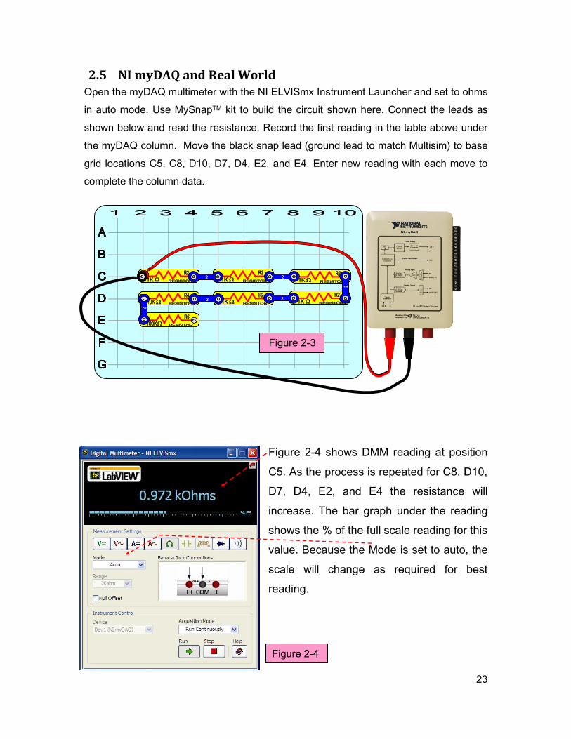
2.5 NI myDAQ and Real World Open the myDAQ multimeter with the NI ELVISmx Instrument Launcher and set to ohms

in auto mode. Use MySnapTM kit to build the circuit shown here. Connect the leads as

shown below and read the resistance. Record the first reading in the table above under

the myDAQ column. Move the black snap lead (ground lead to match Multisim) to base

grid locations C5, C8, D10, D7, D4, E2, and E4. Enter new reading with each move to

complete the column data.

Figure 2-4 shows DMM reading at position

C5. As the process is repeated for C8, D10,

D7, D4, E2, and E4 the resistance will

increase. The bar graph under the reading

shows the % of the full scale reading for this

value. Because the Mode is set to auto, the

scale will change as required for best

reading.

Figure 2-3

Figure 2-4

24

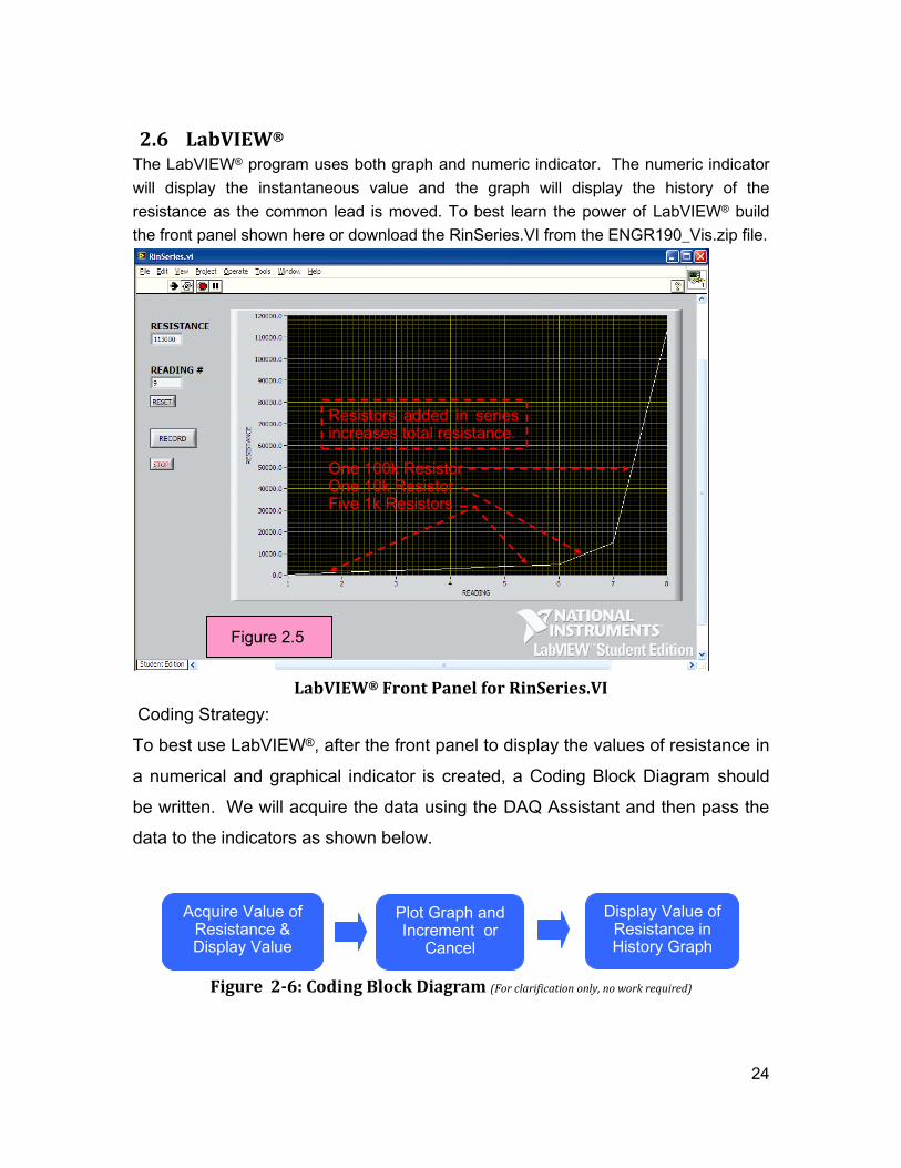
2.6 LabVIEW® The LabVIEW® program uses both graph and numeric indicator. The numeric indicator

will display the instantaneous value and the graph will display the history of the

resistance as the common lead is moved. To best learn the power of LabVIEW® build

the front panel shown here or download the RinSeries.VI from the ENGR190_Vis.zip file.

LabVIEW® Front Panel for RinSeries.VI

Coding Strategy:

To best use LabVIEW®, after the front panel to display the values of resistance in

a numerical and graphical indicator is created, a Coding Block Diagram should

be written. We will acquire the data using the DAQ Assistant and then pass the

data to the indicators as shown below.

Figure 2-6: Coding Block Diagram (For clarification only, no work required)

Acquire Value of Resistance & Display Value

Plot Graph and Increment or

Cancel

Display Value of Resistance in History Graph

Resistors added in series increases total resistance. One 100k Resistor One 10k Resistor Five 1k Resistors

Figure 2.5

25

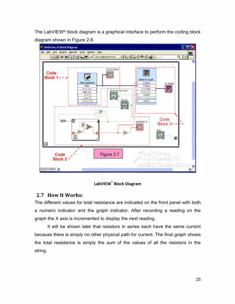
The LabVIEW® block diagram is a graphical interface to perform the coding block

diagram shown in Figure 2-6.

LabVIEW® Block Diagram

2.7 How It Works:

The different values for total resistance are indicated on the front panel with both

a numeric indicator and the graph indicator. After recording a reading on the

graph the X axis is incremented to display the next reading.

It will be shown later that resistors in series each have the same current

because there is simply no other physical path for current. The final graph shows

the total resistance is simply the sum of the values of all the resistors in the

string.

Code Block 1

Code Block 2

Code Block 3

Figure 2.7

26

Lab 02 (Part II): Multisim and Resistors in Parallel

This procedure explains how to use the myDAQ to measure and plot ohms as

resistors are placed in parallel. The resistance will be acquired and plotted using

a similar technique as for resistors in series.

2.8 Topics covered in Lab 02 (Part II)

Objective

Multisim and Circuit Emulation

MyDAQ & Real World

LabVIEW®

Review

2.9 Objective: Use Multisim, LabVIEW®, MySnapTM, and the DMM terminals on the NI myDAQ

to acquire and plot the overall resistance as resistors are added in parallel.

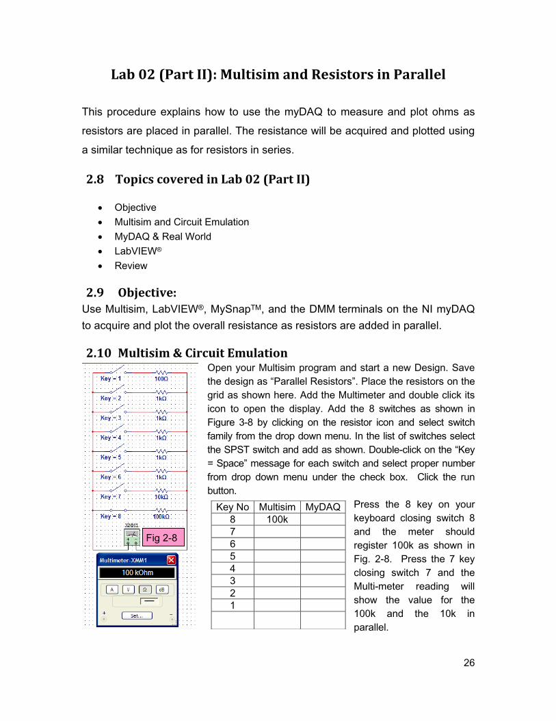
2.10 Multisim & Circuit Emulation Open your Multisim program and start a new Design. Save

the design as “Parallel Resistors”. Place the resistors on the

grid as shown here. Add the Multimeter and double click its

icon to open the display. Add the 8 switches as shown in

Figure 3-8 by clicking on the resistor icon and select switch

family from the drop down menu. In the list of switches select

the SPST switch and add as shown. Double-click on the “Key

= Space” message for each switch and select proper number

from drop down menu under the check box. Click the run

button.

Press the 8 key on your

keyboard closing switch 8

and the meter should

register 100k as shown in

Fig. 2-8. Press the 7 key

closing switch 7 and the

Multi-meter reading will

show the value for the

100k and the 10k in

parallel.

Key No Multisim MyDAQ

8 100k

7

6

5

4

3

2

1

Fig 2-8

27

The meter reading should change to 9.091k. After recording this ON WORKSHEET in

Table 2-2 next to Key 7, press key 6 on your keyboard. This puts the bottom

three resistors in Parallel. Repeat the process until all the resistors are in parallel

and their equivalent resistances have been recorded. While the program is

running you can open and close different switches to see what the parallel

resistance is for the resistors attached to the closed switches.

THE POWER AND SIMPLICITY OF MULTISIM CAN ONLY BE APPRECIATED

BY USING THE PROGRAM TO BUILD AND RUN CIRCUITS. FOR THIS

REASON THE MULTISIM PROGRAMS ARE NOT INCLUDED ON DISC.

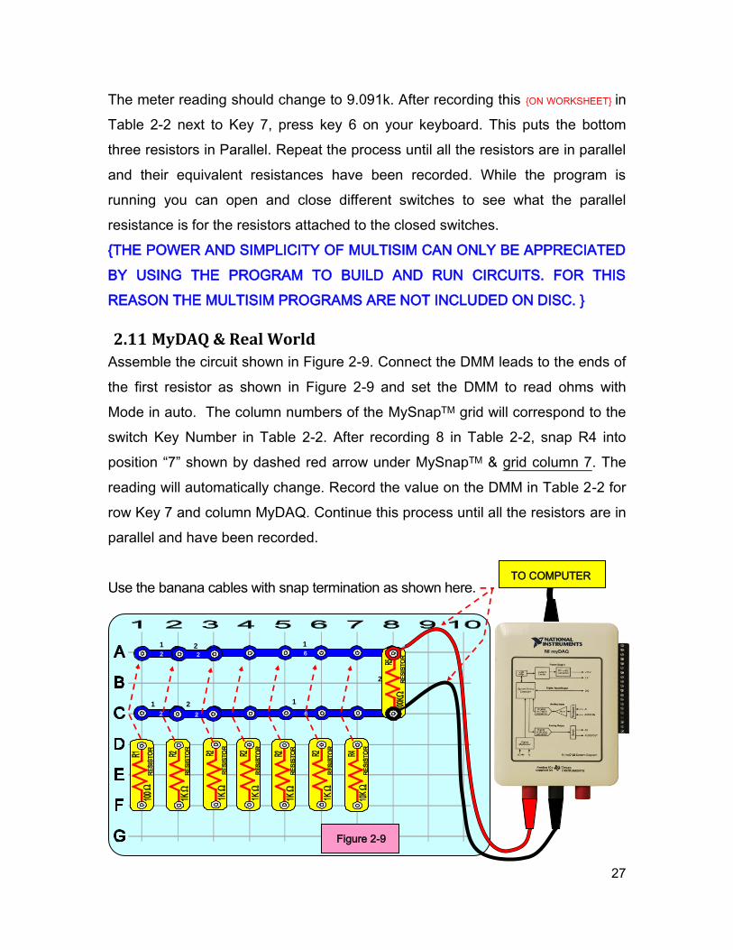
2.11 MyDAQ & Real World

Assemble the circuit shown in Figure 2-9. Connect the DMM leads to the ends of

the first resistor as shown in Figure 2-9 and set the DMM to read ohms with

Mode in auto. The column numbers of the MySnapTM grid will correspond to the

switch Key Number in Table 2-2. After recording 8 in Table 2-2, snap R4 into

position “7” shown by dashed red arrow under MySnapTM & grid column 7. The

reading will automatically change. Record the value on the DMM in Table 2-2 for

row Key 7 and column MyDAQ. Continue this process until all the resistors are in

parallel and have been recorded.

Use the banana cables with snap termination as shown here.

TO COMPUTER

Figure 2-9

1 1

1 1 2

2

2

28

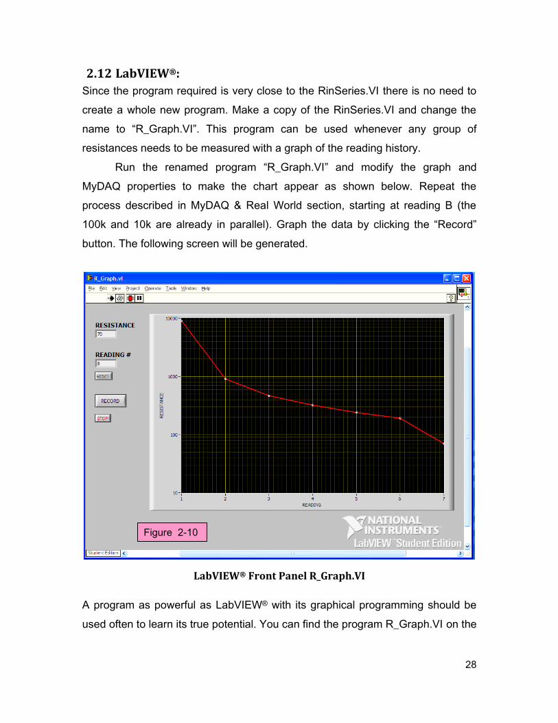
2.12 LabVIEW®:

Since the program required is very close to the RinSeries.VI there is no need to

create a whole new program. Make a copy of the RinSeries.VI and change the

name to “R_Graph.VI”. This program can be used whenever any group of

resistances needs to be measured with a graph of the reading history.

Run the renamed program “R_Graph.VI” and modify the graph and

MyDAQ properties to make the chart appear as shown below. Repeat the

process described in MyDAQ & Real World section, starting at reading B (the

100k and 10k are already in parallel). Graph the data by clicking the “Record”

button. The following screen will be generated.

LabVIEW® Front Panel R_Graph.VI

A program as powerful as LabVIEW® with its graphical programming should be

used often to learn its true potential. You can find the program R_Graph.VI on the

Figure 2-10

29

MySnapTM disc for inspection and comparison to your work. LabVIEW programs

take a few minutes to load. Do not load again when a load is in progress.

2.13 Review

In this Section you emulated series and parallel resistive circuits in Multisim and

studied their properties. Design engineers do this frequently in the course of

investigation for the best circuit to be used in a product. Multisim also provides

the engineer with many tools for detailed observance as circuits are under

construction and investigation. You then used the myDAQ digital multi-meter to

measure real world resistive circuits similar to the ones constructed in Multisim.

Design engineers also build prototypes to test their circuit designs. MySnapTM

provides the engineer with physical components that quickly snap into place to

prototype circuits in the real world. Finally you used LabVIEW® to record your

reading history as you checked the values in the real world example. Engineers

use LabVIEW® to measure final products and graph variances that pick out failures

or defects in manufacturing. Later in this course you will use LabVIEW® to monitor

conditions measured by test equipment and make decisions that are needed for

those conditions. It is a small step, but you have just begun to,

“DO ENGINEERING!”

30

Lab 03: Voltage Generators and Viewers

This portion explains using the Function Generator and Oscilloscope in myDAQ to study

and observe the effect of voltages that produce current in the MySnapTM components.


Objective

What you need

Definitions

Water Pipe Analogy

Building the Lab: DC and AC Voltage Sources

Summary

3.2 Objective:

Use myDAQ devices to produce and study different voltages on a computer, and

then use myDAQ devices to measure and observe these voltages as they are

applied to components on the MySnap™ base. Real life applications apply to any

occupation that works with voltage.

3.3 What You Need:

NI myDAQ


NI ELVISmx Instrument Launcher

Computer System with above software installed

3.4 Definitions

Voltage (V) is a measure of the energy available to move an electric charge from

one point to another or the “Electro Motive Force (EMF)” between those points.

31

There are two different types of voltage in common use today. Direct current

(DC) that moves the current in only one direction, and Alternating current (AC)

that reverses direction periodically, usually many times per second.

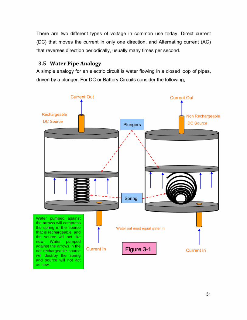
3.5 Water Pipe Analogy

A simple analogy for an electric circuit is water flowing in a closed loop of pipes,

driven by a plunger. For DC or Battery Circuits consider the following;

Rechargeable

DC Source

Current Out

Current In Current In

Water out must equal water in.

- -

Figure 3-1

Plungers

Spring

s

Water pumped against the arrows will compress the spring in the source that is rechargeable, and the source will act like new. Water pumped against the arrows in the not rechargeable source will destroy the spring and source will not act as new.

Non Rechargeable

DC Source

Current Out

32

DC Source +

-

Figure 3-3

Rod at Top Dead Center or Zero Degrees

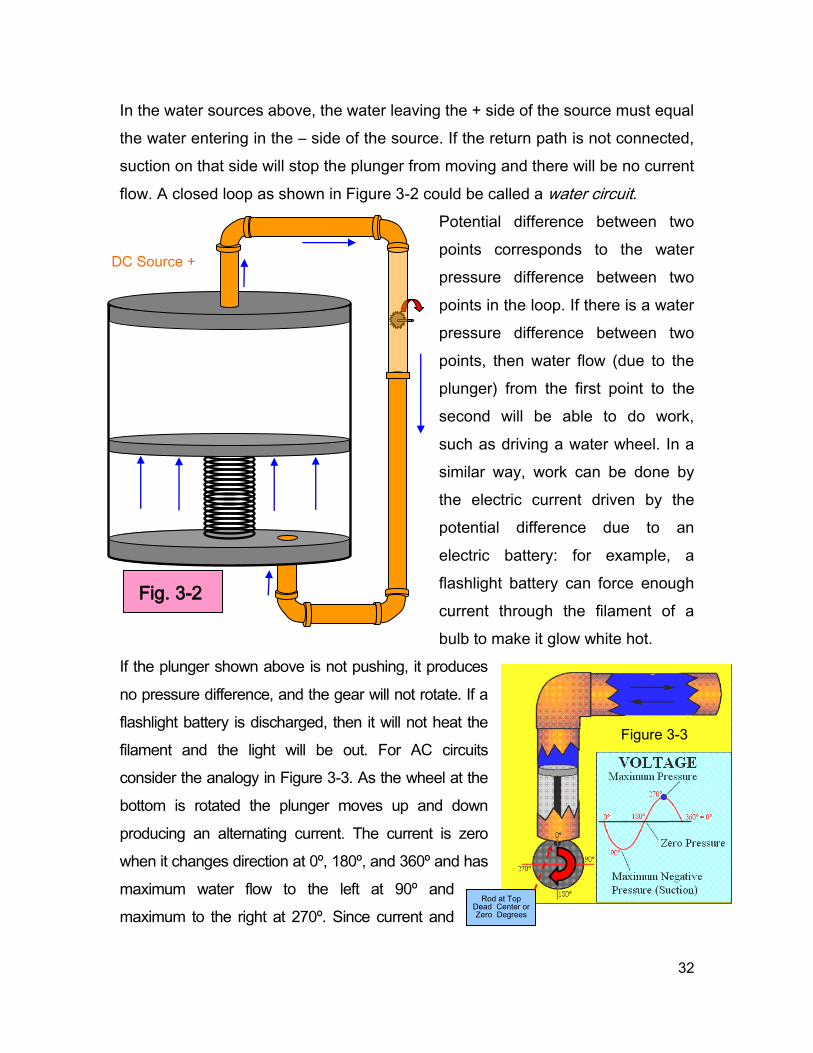
In the water sources above, the water leaving the + side of the source must equal

the water entering in the – side of the source. If the return path is not connected,

suction on that side will stop the plunger from moving and there will be no current

flow. A closed loop as shown in Figure 3-2 could be called a water circuit.

Potential difference between two

points corresponds to the water

pressure difference between two

points in the loop. If there is a water

pressure difference between two

points, then water flow (due to the

plunger) from the first point to the

second will be able to do work,

such as driving a water wheel. In a

similar way, work can be done by

the electric current driven by the

potential difference due to an

electric battery: for example, a

flashlight battery can force enough

current through the filament of a

bulb to make it glow white hot.

If the plunger shown above is not pushing, it produces

no pressure difference, and the gear will not rotate. If a

flashlight battery is discharged, then it will not heat the

filament and the light will be out. For AC circuits

consider the analogy in Figure 3-3. As the wheel at the

bottom is rotated the plunger moves up and down

producing an alternating current. The current is zero

when it changes direction at 0º, 180º, and 360º and has

maximum water flow to the left at 90º and

maximum to the right at 270º. Since current and

Fig. 3-2

33

voltage are in phase for resistors, the voltage across a resistor would appear as shown

in Figure 3.3.

These water flow analogies are useful ways of understanding many electrical

concepts. In such a system, the work done to move water is equal to the pressure

multiplied by the volume of water moved. Similarly, in an electrical circuit, the

work done to move electrons or other charge-carriers is equal to "electrical

pressure" (an old term for voltage) multiplied by the quantity of electrical charge

moved. Voltage is a convenient way of measuring the ability to do work. In

relation to "flow", the larger the "pressure difference" between two points

(potential difference or water pressure difference) the greater the flow between

them (either electric current or water flow).

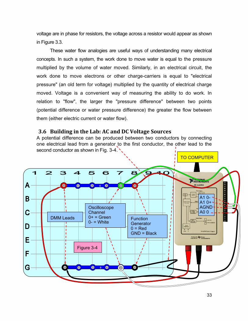
3.6 Building in the Lab: AC and DC Voltage Sources A potential difference can be produced between two conductors by connecting

one electrical lead from a generator to the first conductor, the other lead to the

second conductor as shown in Fig. 3-4.

TO COMPUTER

Figure 3-4

Function Generator 0 = Red GND = Black

Oscilloscope Channel 0+ = Green 0- = White

DMM Leads

A1 0- A1 0+ AGND A0 0

34

After inserting the socket with screw connectors into your myDAQ attach the

leads by turning screw counter-clockwise several turns, place wire under screw,

and tighten by turning screw clockwise until tight. Then build the MySnapTM

circuit as shown above.

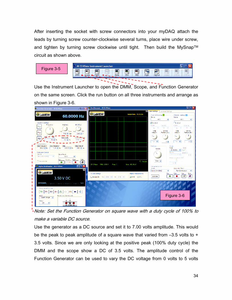
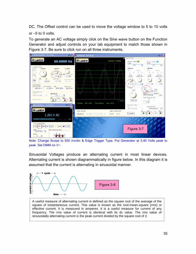
Use the Instrument Launcher to open the DMM, Scope, and Function Generator

on the same screen. Click the run button on all three instruments and arrange as

shown in Figure 3-6.

Note: Set the Function Generator on square wave with a duty cycle of 100% to

make a variable DC source.

Use the generator as a DC source and set it to 7.00 volts amplitude. This would

be the peak to peak amplitude of a square wave that varied from –3.5 volts to +

3.5 volts. Since we are only looking at the positive peak (100% duty cycle) the

DMM and the scope show a DC of 3.5 volts. The amplitude control of the

Function Generator can be used to vary the DC voltage from 0 volts to 5 volts

Figure 3-5

Figure 3-6

35

DC. The Offset control can be used to move the voltage window to 5 to 10 volts

or –5 to 0 volts.

To generate an AC voltage simply click on the Sine wave button on the Function

Generator and adjust controls on your lab equipment to match those shown in

Figure 3-7. Be sure to click run on all three instruments.

Note: Change Scope to 500 mv/div & Edge Trigger Type. Put Generator at 3.40 Volts peak to

peak. Set DMM on V~.

Sinusoidal Voltages produce an alternating current in most linear devices.

Alternating current is shown diagrammatically in figure below. In this diagram it is

assumed that the current is alternating in sinusoidal manner.

A useful measure of alternating current is defined as the square root of the average of the square of instantaneous current. This value is known as the root-mean-square (rms) or effective current. It is measured in amperes. It is a useful measure for current of any frequency. The rms value of current is identical with its dc value. The rms value of sinusoidally alternating current is the peak current divided by the square root of 2.

Figure 3-8

Figure 3-7

36

Notice that a voltage of 1.20 rms has a peak to peak value of 3.40 volts. This

means that the 120 volts in a common household outlet has a peak to peak

voltage of 340 volts.

Because of the high voltage present in electrical outlets the following

warning must be obeyed at all times.

3.7 Summary

You have just built an electronics lab with variable power sources, Digital

measurement equipment, Analog measurement capability, and snap together

prototype capability. You used this lab to generate a variable DC voltage, a

variable AC voltage, and measured both with the DMM and Scope. After a few

improvements to the power source, this lab will be used to investigate the AC

and DC characteristics of electronic circuits and electronic components.

WARNING: SHOCK HAZARD

Never connect any component or lead to electrical outlets in any way !

37

Lab 04: Ohms Law

This portion explains using Multisim, myDAQ, LabVIEW®, and MySnapTM to study Ohms

Law for resistors using DC and AC voltages and currents.


Objective

What You Need

Ohms Law

Multisim: Virtual World

MySnap™: Real World

Hardware Limits

Summary

Know Your Equipment Review

4.2 Objective:

Use Multisim to emulate and study Ohm’s Law on a computer, and then use

myDAQ to measure and observe the same circuit built in the real world on the

MySnap™ base. Real life applications apply to any occupation that uses

electronic circuits and the engineering of those circuits.

4.3 What You Need:

Multisim

NI myDAQ

LabVIEW®


Computer System with above software installed.

38

4.4 Ohms Law:

A common use of the term "voltage" is in describing the voltage dropped across

an electrical device (such as a resistor). The voltage drop across the device can

be understood as the difference between measurements at each terminal of the

device with respect to a common reference point (or ground).

Ohm's law states that current through a resistive component is directly

proportional to the voltage across the component, and inversely proportional to

the resistance of the component.

Mathematically:

I = V/R or V = IR or R = V/I

Where, I is the current through the component in units of amperes, V is the

voltage measured across the component in units of volts, and R is the resistance

of the component in units of ohms. The symbol for ohms =

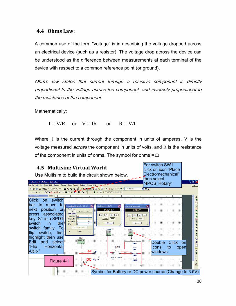
4.5 Multisim: Virtual World

Use Multisim to build the circuit shown below.

Double Click on Icons to open windows.

Figure 4-1

Symbol for Battery or DC power source (Change to 3.5V).

AC

DC

Click on switch bar to move to next position or press associated key. S1 is a SPDT switch in the switch family. To flip switch, first highlight then use Edit and select “Flip Horizontal Alt+x”

For switch SW1 click on icon “Place Electromechanical” then select “4POS_Rotary”

39

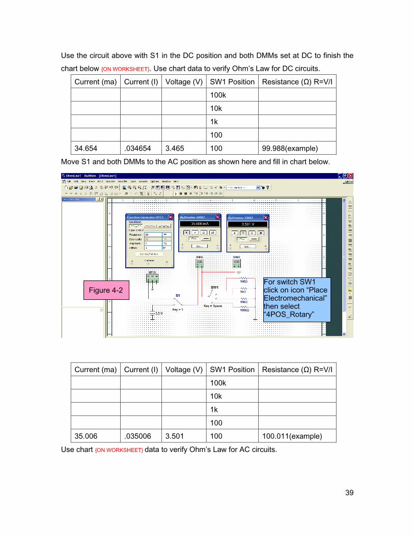
Use the circuit above with S1 in the DC position and both DMMs set at DC to finish the

chart below ON WORKSHEET. Use chart data to verify Ohm’s Law for DC circuits.

Current (ma) Current (I) Voltage (V) SW1 Position Resistance (Ω) R=V/I

100k

10k

1k

100

34.654 .034654 3.465 100 99.988(example)

Move S1 and both DMMs to the AC position as shown here and fill in chart below.


100k

10k

1k

100

35.006 .035006 3.501 100 100.011(example)

Use chart ON WORKSHEET data to verify Ohm’s Law for AC circuits.

Figure 4-2 For switch SW1 click on icon “Place Electromechanical” then select “4POS_Rotary”

40

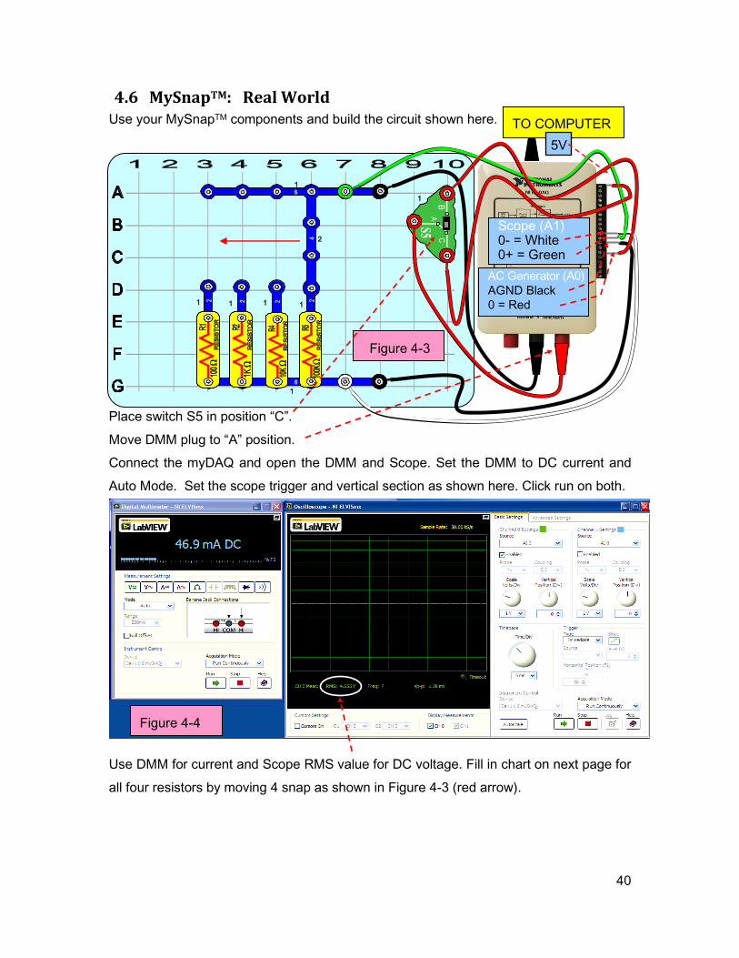
4.6 MySnapTM: Real World Use your MySnapTM components and build the circuit shown here.

Place switch S5 in position “C”.

Move DMM plug to “A” position.

Connect the myDAQ and open the DMM and Scope. Set the DMM to DC current and

Auto Mode. Set the scope trigger and vertical section as shown here. Click run on both.

Use DMM for current and Scope RMS value for DC voltage. Fill in chart on next page for

all four resistors by moving 4 snap as shown in Figure 4-3 (red arrow).

Figure 4-4

TO COMPUTER

Figure 4-3

AC Generator (A0)

AGND Black

0 = Red

Scope (A1) 0- = White 0+ = Green

1

1 1 1 1

1

2

1

5V

41

TABLES FOUND ON WORKSHEET LAST PAGE OF THIS MANUAL

Current (ma) Current (I) Voltage (V) R Position Ohms (Ω) R=V/I

100k

10k

1k

100

46.9 .0469 4.655 100 99.254(example)

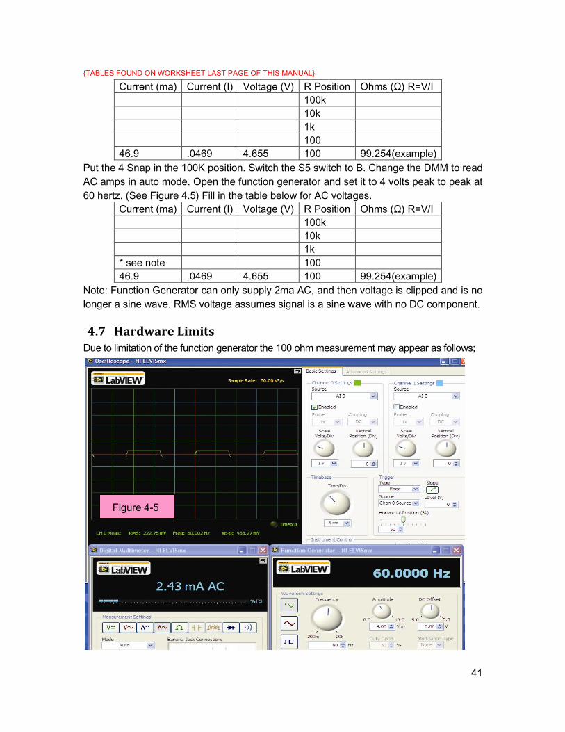
Put the 4 Snap in the 100K position. Switch the S5 switch to B. Change the DMM to read

AC amps in auto mode. Open the function generator and set it to 4 volts peak to peak at

60 hertz. (See Figure 4.5) Fill in the table below for AC voltages.


100k

10k

1k

* see note 100

46.9 .0469 4.655 100 99.254(example)

Note: Function Generator can only supply 2ma AC, and then voltage is clipped and is no

longer a sine wave. RMS voltage assumes signal is a sine wave with no DC component.

4.7 Hardware Limits Due to limitation of the function generator the 100 ohm measurement may appear as follows;

Figure 4-5

42

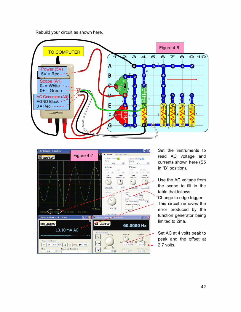
Rebuild your circuit as shown here.

Set the instruments to read AC voltage and current as shown here (S5 in “B” position).

Set the instruments to

read AC voltage and

currents shown here (S5

in “B” position).

Use the AC voltage from

the scope to fill in the

table that follows.

Change to edge trigger.

This circuit removes the

error produced by the

function generator being

limited to 2ma.

Set AC at 4 volts peak to

peak and the offset at

2.7 volts.

Figure 4-7

TO COMPUTER Figure 4-6

AC Generator (A0)

AGND Black

0 = Red

Scope (A1) 0- = White 0+ = Green

Power (5V) 5V = Red

1

1

1

1

1 1 1 1

1

1

2

2 2 2 2

2

2

2

2

43

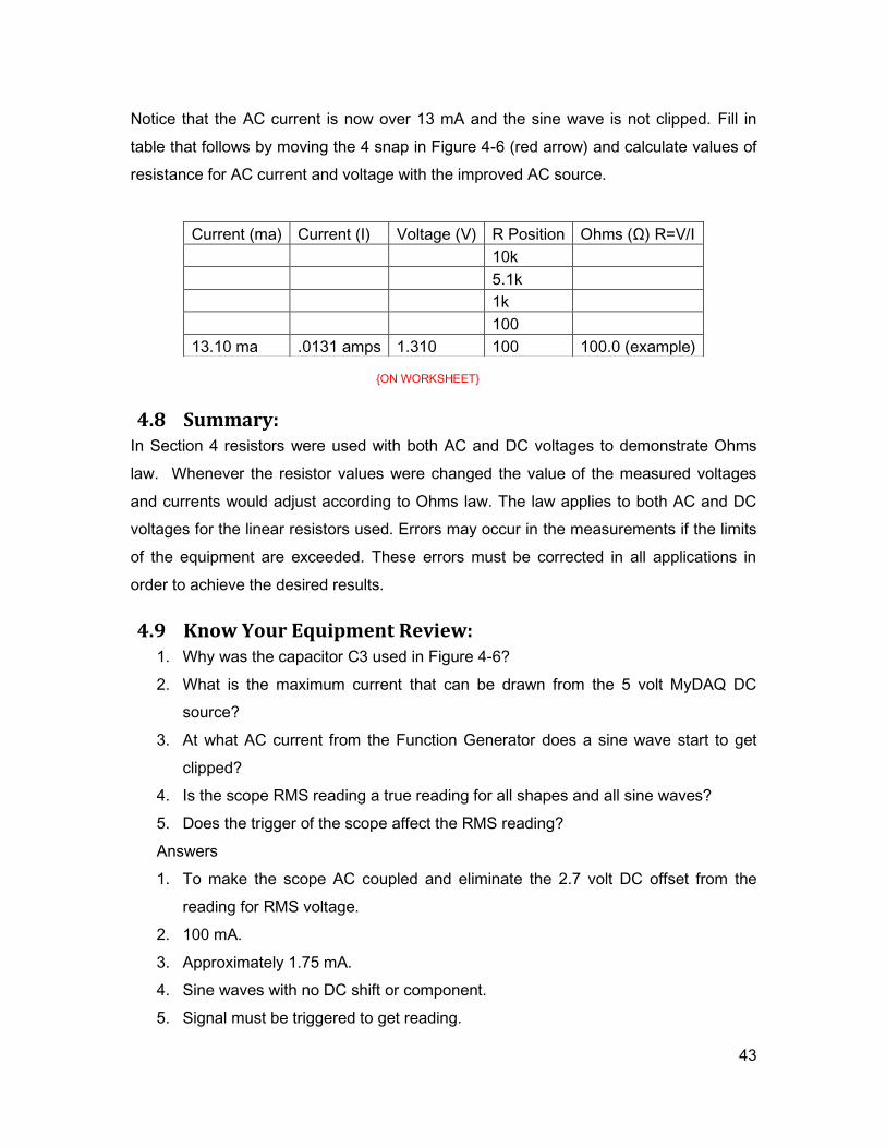
Notice that the AC current is now over 13 mA and the sine wave is not clipped. Fill in

table that follows by moving the 4 snap in Figure 4-6 (red arrow) and calculate values of

resistance for AC current and voltage with the improved AC source.

4.8 Summary: In Section 4 resistors were used with both AC and DC voltages to demonstrate Ohms

law. Whenever the resistor values were changed the value of the measured voltages

and currents would adjust according to Ohms law. The law applies to both AC and DC

voltages for the linear resistors used. Errors may occur in the measurements if the limits

of the equipment are exceeded. These errors must be corrected in all applications in

order to achieve the desired results.

4.9 Know Your Equipment Review: 1. Why was the capacitor C3 used in Figure 4-6?

2. What is the maximum current that can be drawn from the 5 volt MyDAQ DC

source?

3. At what AC current from the Function Generator does a sine wave start to get

clipped?

4. Is the scope RMS reading a true reading for all shapes and all sine waves?

5. Does the trigger of the scope affect the RMS reading?

Answers

1. To make the scope AC coupled and eliminate the 2.7 volt DC offset from the

reading for RMS voltage.

2. 100 mA.

3. Approximately 1.75 mA.

4. Sine waves with no DC shift or component.

5. Signal must be triggered to get reading.


10k

5.1k

1k

100

13.10 ma .0131 amps 1.310 100 100.0 (example)

ON WORKSHEET

44

Lab 05: Kirchhoff's Voltage Law

The Kirchhoff’s voltage law is one of two fundamental laws in electrical

engineering developed by German physicist Gustav Robert Kirchhoff in 1845.

The Kirchhoff’s voltage law states

“The sum of the electrical potentials (voltages) around any closed circuit is zero.”

This portion explains using a National Instruments myDAQ to measure voltages

around a closed circuit. The measurements will be taken with the myDAQ DMM.

The components to be measured are supplied in the MySnap™ model “BASIC

ELECTRONICS EE100”. Real life applications apply to any occupation that uses

electrical components with measurement equipment.

5.1 Topic covered in Lab 05

Objective

What You Need

The Circuit

Multisim Verification of Kirchhoff’s Voltage Law (KVL)

MyDAQ DMM Measurements

Sources for Error

5.2 Objective:

Use Multisim, the DMM in the NI myDAQ, and MySnapTM to measure and record

both DC and AC voltage sums around a closed circuit loop and thus verify

Kirchhoff’s Voltage Law.

5.3 What You Need:

Multisim

NI myDAQ


Computer System with NI software installed

45

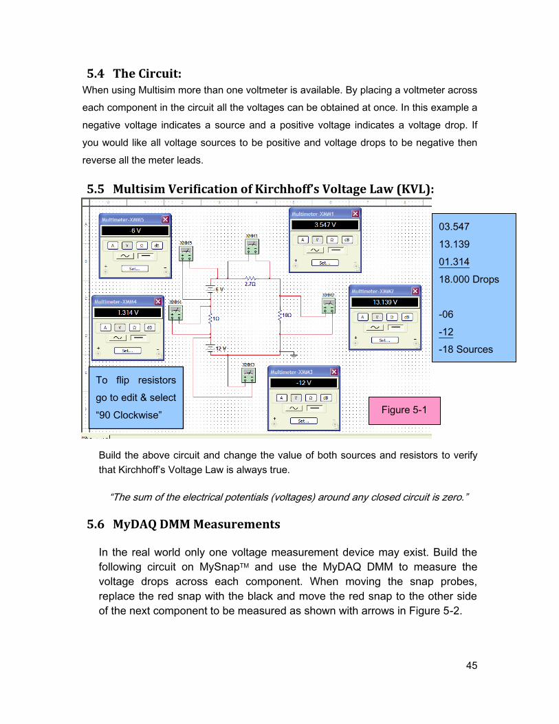
5.4 The Circuit: When using Multisim more than one voltmeter is available. By placing a voltmeter across

each component in the circuit all the voltages can be obtained at once. In this example a

negative voltage indicates a source and a positive voltage indicates a voltage drop. If

you would like all voltage sources to be positive and voltage drops to be negative then

reverse all the meter leads.

5.5 Multisim Verification of Kirchhoff’s Voltage Law (KVL):

Build the above circuit and change the value of both sources and resistors to verify

that Kirchhoff’s Voltage Law is always true.

“The sum of the electrical potentials (voltages) around any closed circuit is zero.”

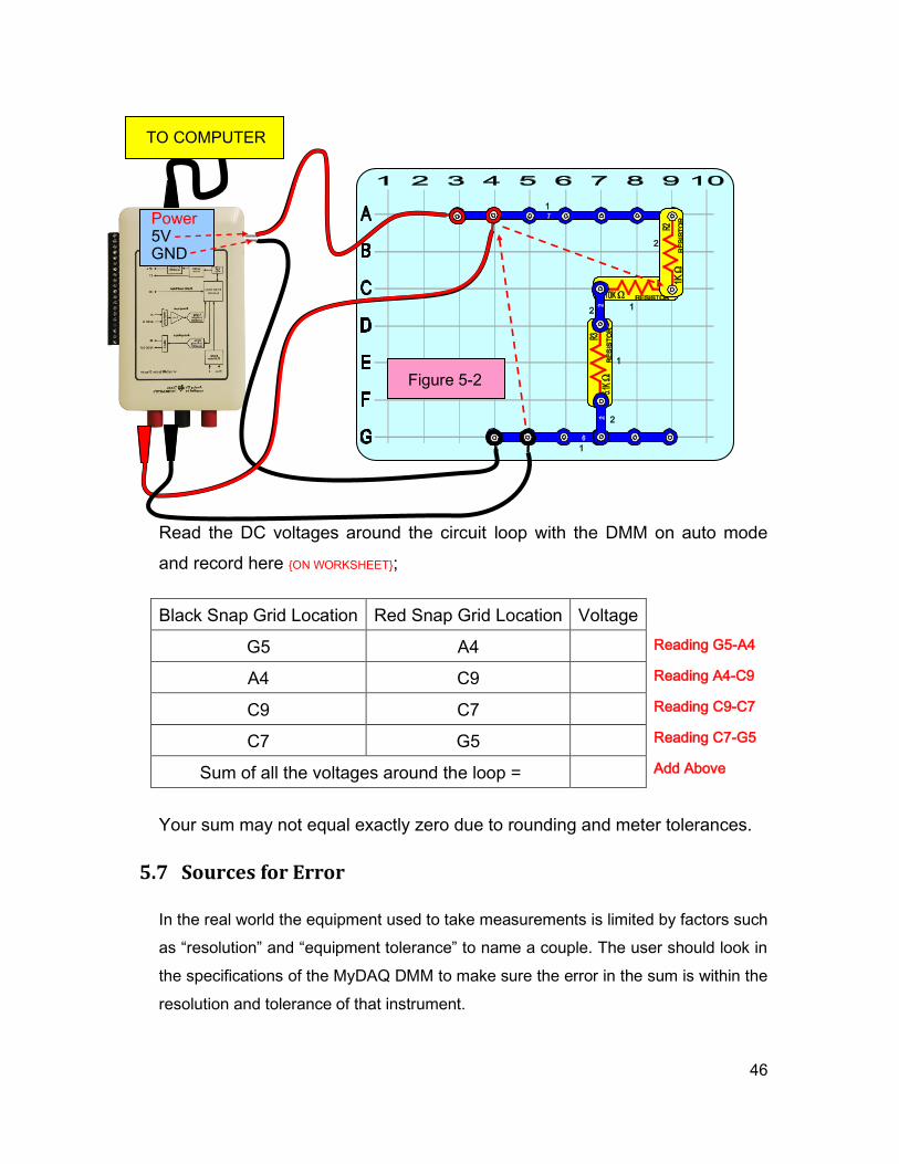
5.6 MyDAQ DMM Measurements

In the real world only one voltage measurement device may exist. Build the

following circuit on MySnapTM and use the MyDAQ DMM to measure the

voltage drops across each component. When moving the snap probes,

replace the red snap with the black and move the red snap to the other side

of the next component to be measured as shown with arrows in Figure 5-2.

03.547

13.139

01.314

18.000 Drops

-06

-12

-18 Sources

18-18=0 (KVL)

Figure 5-1

To flip resistors

go to edit & select

“90 Clockwise”

46

Read the DC voltages around the circuit loop with the DMM on auto mode

and record here ON WORKSHEET;

Black Snap Grid Location Red Snap Grid Location Voltage

G5 A4

A4 C9

C9 C7

C7 G5

Sum of all the voltages around the loop =

Your sum may not equal exactly zero due to rounding and meter tolerances.

5.7 Sources for Error

In the real world the equipment used to take measurements is limited by factors such

as “resolution” and “equipment tolerance” to name a couple. The user should look in

the specifications of the MyDAQ DMM to make sure the error in the sum is within the

resolution and tolerance of that instrument.

TO COMPUTER

Figure 5-2

Power 5V GND

1

1

1

1

2

2

2

Reading G5-A4

Reading A4-C9

Reading C9-C7

Reading C7-G5

Add Above

47

Lab 06: Capacitors

The capacitor is an electrical device characterized by its capacity to store an

electric charge, pass AC, block DC, and change the phase relationship between

current and voltage in a circuit. This section will explain capacitors using

analogies, virtual capacitors using Multisim, real capacitors using MySnapTM and

circuits that demonstrate their properties. In the real world, measurements will

be taken with the myDAQ DMM and their properties observed with the MyDAQ

scope. The components to be measured are supplied in the MySnap™ model

“BASIC ELECTRONICS EE100”. Real life applications apply to power supplies,

appliances, television, cell phones, satellite receivers, and almost anything

electronic.


Objective

What you need

Water Pipe Analogy

Understanding Capacitor Properties

Multisim Capacitor Circuit

More About Capacitor Properties

Transient Responses

RC time constant

The Real World - MySnapTM

Actual Values and Tolerances

LabVIEW® RC meter

How it Works

Review

6.2 Objective:

Use Multisim, the NI myDAQ, LabVIEW®, and MySnapTM to investigate both DC

and AC properties of electronic capacitors. Introduce transient responses and

phase relationship between current and voltage.

48

Maximum I into Pipe =

Maximum V across R

Maximum I from Pipe =

Maximum -V across R

6.3 What You Need:

Multisim

NI myDAQ



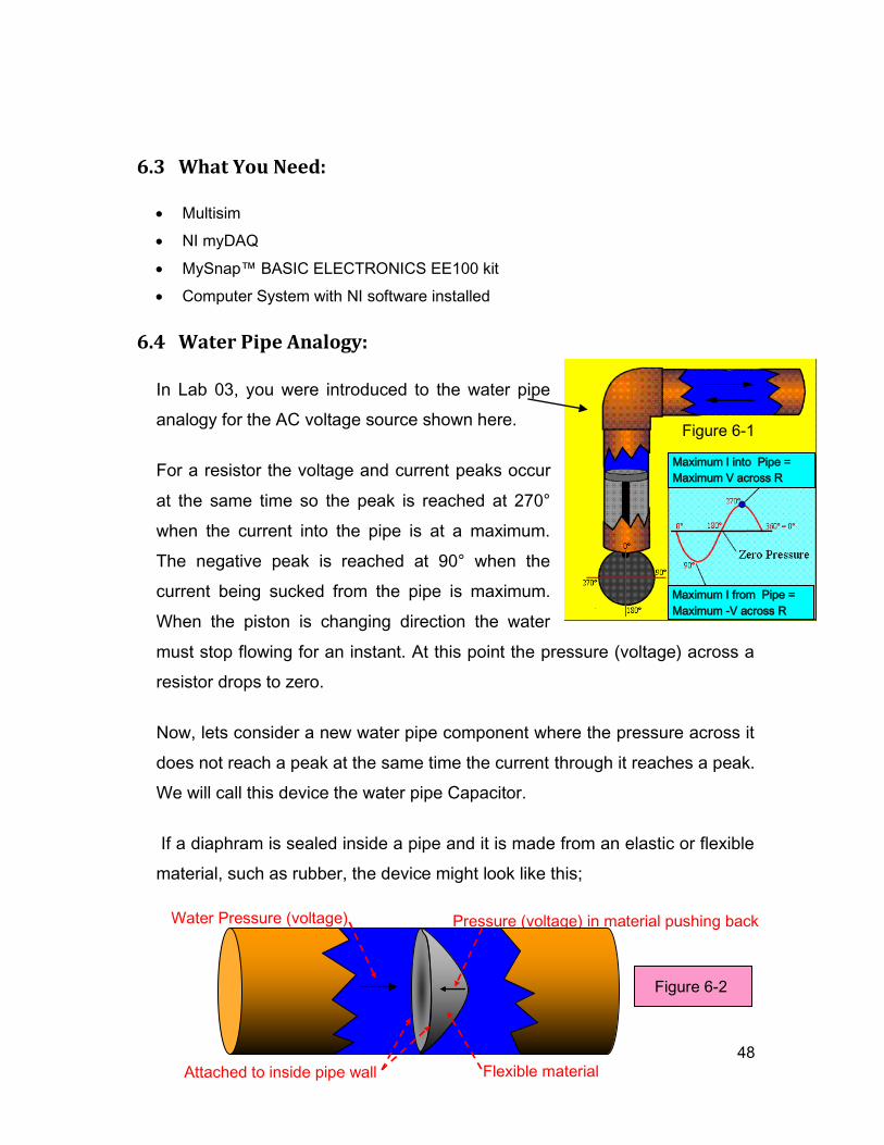
6.4 Water Pipe Analogy:

In Lab 03, you were introduced to the water pipe

analogy for the AC voltage source shown here.

For a resistor the voltage and current peaks occur

at the same time so the peak is reached at 270°

when the current into the pipe is at a maximum.

The negative peak is reached at 90° when the

current being sucked from the pipe is maximum.

When the piston is changing direction the water

must stop flowing for an instant. At this point the pressure (voltage) across a

resistor drops to zero.

Now, lets consider a new water pipe component where the pressure across it

does not reach a peak at the same time the current through it reaches a peak.

We will call this device the water pipe Capacitor.

If a diaphram is sealed inside a pipe and it is made from an elastic or flexible

material, such as rubber, the device might look like this;

Pressure (voltage) in material pushing back

Figure 6-1

Attached to inside pipe wall Flexible material

Water Pressure (voltage)

Figure 6-2

49

If the total drops of water = Q and the pressure in the material pushing back =

V we could define the value of the capacitor (C) as;

6.5 Understanding Capacitor Properties:

The relationship between water flow (current) and back pressure (voltage)

shows that water must flow FIRST in order to produce a back pressure.

Therefore the current leads the back pressure (voltage). They no longer occur

at the same time as in the resistor. To better see this relationship, play the

animated gif file called Cap.gif on the disc that came with the MySnapTM

parts. It can be viewed using a player such as “Windows Media Player”,

“Windows Picture and Fax Viewer” or “QuickTime” just to name a few. Points

of interest that should be noted in the analogies are;

Water flow (current) leads the Back Pressure (voltage) by 90°.

Alternating water flow (AC) passes through the capacitor easily.

When a Capacitor stores water (charge) a back pressure (voltage) exist.

One way water flow (DC) is blocked by capacitor when back pressure

(voltage on C) = forward pump pressure (battery voltage).

It takes time for a Capacitor to charge (water must enter diaphram).

Maximum AC current occurs when there is no back pressure.

Peak back pressure occurs when AC current changes direction.

Size and material can change Capacitors properties.

An electronic capacitor consists of two conductive surfaces (plates) separated by

a non-conductive material called the dielectric. The plates hold equal and

opposite charges on their facing surfaces, and the dielectric develops an electric

field. In SI units, a capacitance of 1 Farad (F) means that 1 Coulomb of charge

on each plate produces a voltage of 1 Volt across the Capacitor. If an electronic

capacitor is represented by the constant C, then the ratio of charge ±Q on each

plate to the voltage V between them defines the Capacitor as:

C = Q Number of Drops of Water

V Back Pressure due to Stretching

C = Q Charge on each plate

V Electric field in dielectric

50

Figure 6-3

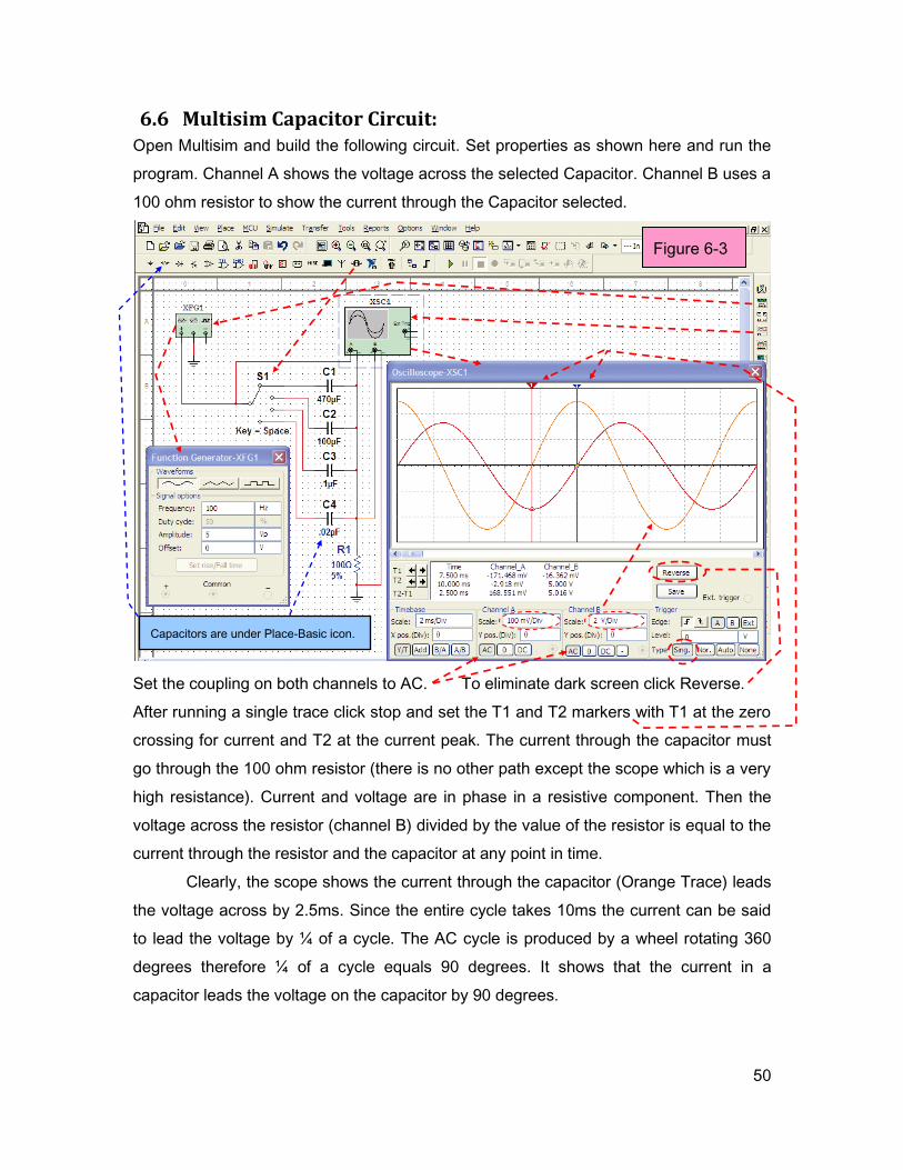
6.6 Multisim Capacitor Circuit: Open Multisim and build the following circuit. Set properties as shown here and run the

program. Channel A shows the voltage across the selected Capacitor. Channel B uses a

100 ohm resistor to show the current through the Capacitor selected.

Set the coupling on both channels to AC. To eliminate dark screen click Reverse.

After running a single trace click stop and set the T1 and T2 markers with T1 at the zero

crossing for current and T2 at the current peak. The current through the capacitor must

go through the 100 ohm resistor (there is no other path except the scope which is a very

high resistance). Current and voltage are in phase in a resistive component. Then the

voltage across the resistor (channel B) divided by the value of the resistor is equal to the

current through the resistor and the capacitor at any point in time.

Clearly, the scope shows the current through the capacitor (Orange Trace) leads

the voltage across by 2.5ms. Since the entire cycle takes 10ms the current can be said

to lead the voltage by ¼ of a cycle. The AC cycle is produced by a wheel rotating 360

degrees therefore ¼ of a cycle equals 90 degrees. It shows that the current in a

capacitor leads the voltage on the capacitor by 90 degrees.

Capacitors are under Place-Basic icon.

51

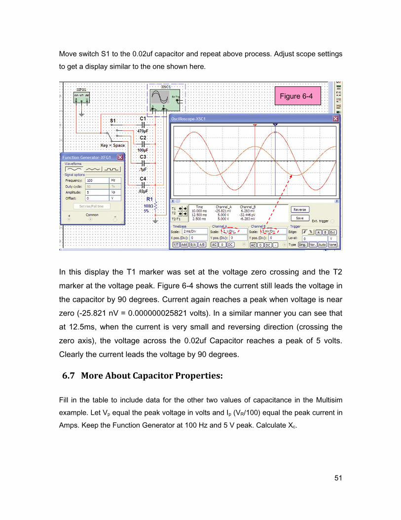
Move switch S1 to the 0.02uf capacitor and repeat above process. Adjust scope settings

to get a display similar to the one shown here.

In this display the T1 marker was set at the voltage zero crossing and the T2

marker at the voltage peak. Figure 6-4 shows the current still leads the voltage in

the capacitor by 90 degrees. Current again reaches a peak when voltage is near

zero (-25.821 nV = 0.000000025821 volts). In a similar manner you can see that

at 12.5ms, when the current is very small and reversing direction (crossing the

zero axis), the voltage across the 0.02uf Capacitor reaches a peak of 5 volts.

Clearly the current leads the voltage by 90 degrees.

6.7 More About Capacitor Properties:

Fill in the table to include data for the other two values of capacitance in the Multisim

example. Let Vp equal the peak voltage in volts and Ip (VR/100) equal the peak current in

Amps. Keep the Function Generator at 100 Hz and 5 V peak. Calculate Xc.

Figure 6-4

52

Figure 6-5

ON WORKSHEET

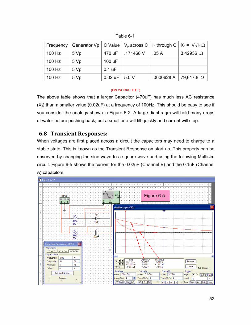
The above table shows that a larger Capacitor (470uF) has much less AC resistance

(Xc) than a smaller value (0.02uF) at a frequency of 100Hz. This should be easy to see if

you consider the analogy shown in Figure 6-2. A large diaphragm will hold many drops

of water before pushing back, but a small one will fill quickly and current will stop.

6.8 Transient Responses: When voltages are first placed across a circuit the capacitors may need to charge to a

stable state. This is known as the Transient Response on start up. This property can be

observed by changing the sine wave to a square wave and using the following Multisim

circuit. Figure 6-5 shows the current for the 0.02uF (Channel B) and the 0.1uF (Channel

A) capacitors.

Frequency Generator Vp C Value Vp across C Ip through C Xc = Vp/Ip

100 Hz 5 Vp 470 uF .171468 V .05 A 3.42936

100 Hz 5 Vp 100 uF

100 Hz 5 Vp 0.1 uF

100 Hz 5 Vp 0.02 uF 5.0 V .0000628 A 79,617.8

Table 6-1

53

Notice that both capacitors start at exactly the same charging current

(10V/1k=10ma), but the 0.02uF charging current drops to 3.62ma in 20.149us

and the .1uf charging takes five times longer (100us) to drop to the same value

which is a drop of 63.2% from the starting value.

6.9 RC time constant:

This decay (or charge) time is related to the product of the current limiting

resistor and the value of the capacitor (RC). The time required for the current to

fall to I0 / e (63.2% of original value) is called the RC time constant and is given

by the symbol tau as = RC. The symbol e is known as the natural log. It is an

irrational number but we will approximate it as 2.71828. After each RC time

constant the current will decrease by 63.2% of the remaining value during the

next time constant.

Unlike resistance which has a fixed value with frequency, a Capacitors resistance

(called Reactance, and shown as XC in Table 6-1) varies with frequency. As the

frequency applied to the capacitor increases its reactance (measured in ohms)

decreases and as the frequency decreases its reactance increases. Reactance

can be calculated from the equation XC = 1/2fC or 1/C where 2f and f =

frequency in Hertz. Example, using Table 6-1 last row information;

XC = 1/(6.28x100x.02x10-6) = 1/(0.00001256) = 79,617.8 (same as Table6-1 Vp/Ip)

If the frequency is increased by 1000 times (from 100 Hz to 100,000 Hz) the reactance

will drop by 1000 times. The new value becomes;

XC = 1/(6.28x100000x.02x10-6) = 1/(0.01256) = 79.6178 ohms

54

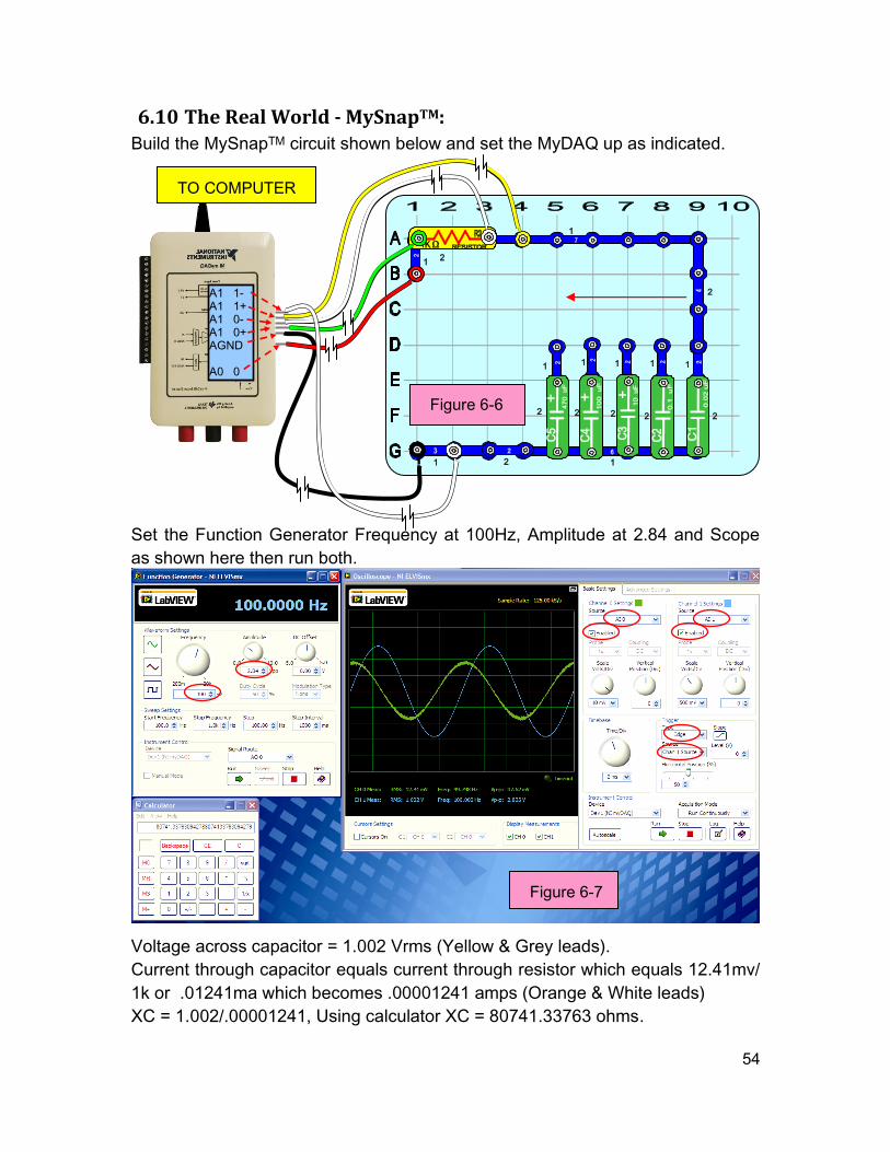
6.10 The Real World - MySnapTM:

Build the MySnapTM circuit shown below and set the MyDAQ up as indicated.

Set the Function Generator Frequency at 100Hz, Amplitude at 2.84 and Scope

as shown here then run both.

Voltage across capacitor = 1.002 Vrms (Yellow & Grey leads).

Current through capacitor equals current through resistor which equals 12.41mv/

1k or .01241ma which becomes .00001241 amps (Orange & White leads)

XC = 1.002/.00001241, Using calculator XC = 80741.33763 ohms.

Figure 6-7

TO COMPUTER

Figure 6-6

A1 1- A1 1+ A1 0- A1 0+ AGND A0 0

1

1

1 1 1 1 1

1 1 2

2

2

2 2 2 2 2

55

Using the reactance just calculated and the equation for reactance, the actual

value of the capacitor can be calculated as follows;

C = 1/(2f XC) = 1/(2)(3.14)(100)(80741.33763) = 1.972 x 10-8 = 0.01972uF

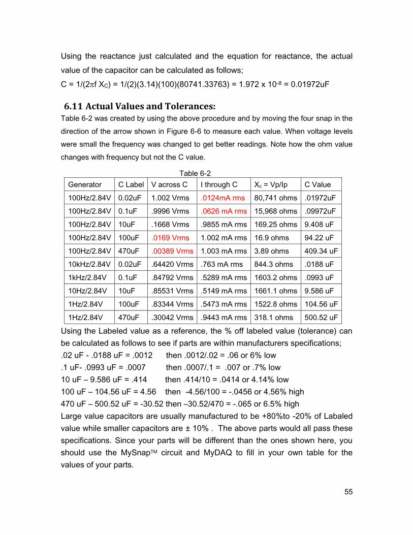
6.11 Actual Values and Tolerances: Table 6-2 was created by using the above procedure and by moving the four snap in the

direction of the arrow shown in Figure 6-6 to measure each value. When voltage levels

were small the frequency was changed to get better readings. Note how the ohm value

changes with frequency but not the C value.

Generator C Label V across C I through C Xc = Vp/Ip C Value

100Hz/2.84V 0.02uF 1.002 Vrms .0124mA rms 80,741 ohms .01972uF

100Hz/2.84V 0.1uF .9996 Vrms .0626 mA rms 15,968 ohms .09972uF

100Hz/2.84V 10uF .1668 Vrms .9855 mA rms 169.25 ohms 9.408 uF

100Hz/2.84V 100uF .0169 Vrms 1.002 mA rms 16.9 ohms 94.22 uF

100Hz/2.84V 470uF .00389 Vrms 1.003 mA rms 3.89 ohms 409.34 uF

10kHz/2.84V 0.02uF .64420 Vrms .763 mA rms 844.3 ohms .0188 uF

1kHz/2.84V 0.1uF .84792 Vrms .5289 mA rms 1603.2 ohms .0993 uF




Using the Labeled value as a reference, the % off labeled value (tolerance) can

be calculated as follows to see if parts are within manufacturers specifications;

.02 uF - .0188 uF = .0012 then .0012/.02 = .06 or 6% low

.1 uF- .0993 uF = .0007 then .0007/.1 = .007 or .7% low

10 uF – 9.586 uF = .414 then .414/10 = .0414 or 4.14% low

100 uF – 104.56 uF = 4.56 then -4.56/100 = -.0456 or 4.56% high

470 uF – 500.52 uF = -30.52 then –30.52/470 = -.065 or 6.5% high

Large value capacitors are usually manufactured to be +80%to -20% of Labaled

value while smaller capacitors are ± 10% . The above parts would all pass these

specifications. Since your parts will be different than the ones shown here, you

should use the MySnapTM circuit and MyDAQ to fill in your own table for the

values of your parts.

Table 6-2

56

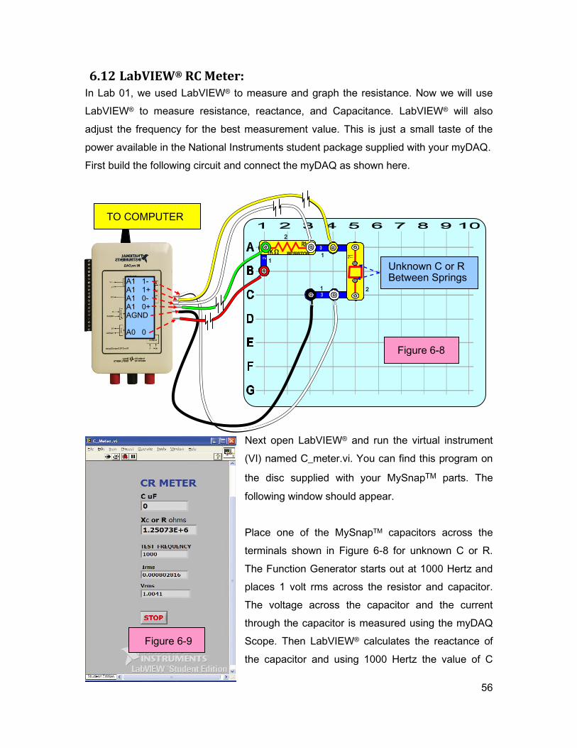
Figure 6-9

6.12 LabVIEW® RC Meter: In Lab 01, we used LabVIEW® to measure and graph the resistance. Now we will use

LabVIEW® to measure resistance, reactance, and Capacitance. LabVIEW® will also

adjust the frequency for the best measurement value. This is just a small taste of the

power available in the National Instruments student package supplied with your myDAQ.

First build the following circuit and connect the myDAQ as shown here.

Next open LabVIEW® and run the virtual instrument

(VI) named C_meter.vi. You can find this program on

the disc supplied with your MySnapTM parts. The

following window should appear.

Place one of the MySnapTM capacitors across the

terminals shown in Figure 6-8 for unknown C or R.

The Function Generator starts out at 1000 Hertz and

places 1 volt rms across the resistor and capacitor.

The voltage across the capacitor and the current

through the capacitor is measured using the myDAQ

Scope. Then LabVIEW® calculates the reactance of

the capacitor and using 1000 Hertz the value of C

TO COMPUTER

Figure 6-8

Unknown C or R Between Springs A1 1-

A1 1+ A1 0- A1 0+ AGND A0 0

1

1

1

2

2

57

required to produce that reactance. If the value of C is greater than 0.6 uF, the frequency

is changed to 10 Hertz and a new measurement and calculation is made and displayed.

When measuring a resistor, the value of C displayed is the value of capacitance that

would have the same reactance at the frequency being used to measure the resistor.

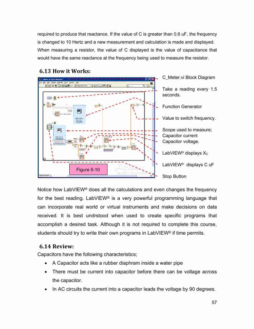
6.13 How it Works: C_Meter.vi Block Diagram

Take a reading every 1.5

seconds.

Function Generator

Value to switch frequency.

Scope used to measure;

Capacitor current

Capacitor voltage.

LabVIEW® displays XC

LabVIEW® displays C uF

Stop Button

Notice how LabVIEW® does all the calculations and even changes the frequency

for the best reading. LabVIEW® is a very powerful programming language that

can incorporate real world or virtual instruments and make decisions on data

received. It is best undrstood when used to create specific programs that

accomplish a desired task. Although it is not required to complete this course,

students should try to write their own programs in LabVIEW® if time permits.

6.14 Review:

Capacitors have the following characteristics;

A Capacitor acts like a rubber diaphram inside a water pipe

There must be current into capacitor before there can be voltage across

the capacitor.

In AC circuits the current into a capacitor leads the voltage by 90 degrees.

Figure 6-10

58

The resistance of a capacitor in AC circuits is called Reactance (XC).

The Reactance of a Capacitor drops when Frequency increases according

to the equation XC = 1/(2fC)

A capacitor blocks Direct Current by charging and producing an equal and

opposite DC voltage.

For DC voltages capacitors produce a “Transient Response” on start up.

The charge time (or discharge time) to 63.2% of final value is called the

RC time constant and is given by the symbol tau as = RC.

Because it takes time to charge a Capacitor, the voltage across a

capacitor cannot be changed instantly as for a resistor.

LabVIEW® can control the virtual instruments in the myDAQ.

LabVIEW® can calculate values and display results using external

measurements.

Some common uses of capacitors are,

Set time delay to turn lights on-off slowly.

Remove AC ripple when converting AC to DC in power supplies.

Tune circuits to receive specific frequencies in radios and TV sets.

Store charges and release later as in flash on cameras.

Supply extra current to help air conditioning motors start.

Act like a battery in small toys to prevent batteries from discharging.

Produce large currents for short period of time as in spot welding.

59

Lab 07: Inductors

The Inductor is an electrical device characterized by its capacity to store energy

in a magnetic field, pass DC, block AC, and change the phase relationship

between current and voltage in a circuit. This lab will explain inductors using

analogies, virtual inductors using Multisim, real inductors using MySnapTM and

circuits that demonstrate their properties. In the real world, measurements will

be taken with the myDAQ DMM and their properties observed with the MyDAQ

scope. The components to be measured are supplied in the MySnap™ model

“BASIC ELECTRONICS EE100”. Real life applications apply to power supplies,

appliances, television, cell phones, satellite receivers, and almost anything

electronic.


Objective

What you need

Water pipe analogy

In electrical circuit

Multisim Inductor Circuit

More About Inductor Properties

Transient Responses

RL time constant

The Real World - MySnapTM

Actual Values and Tolerances

Labview® RLC meter

How it Works

Review

7.2 Objective:


and AC properties of inductors in electronic circuits. Study inductive responses

and phase relationship between current and voltage.

60

7.3 What You Need:

Multisim

NI myDAQ




In lab 06, you were introduced to the water pipe analogy for the Capacitor as

a rubber diaphragm in a water pipe. The inductor can be described as

electrical momentum and can be represented in a water pipe analogy by the

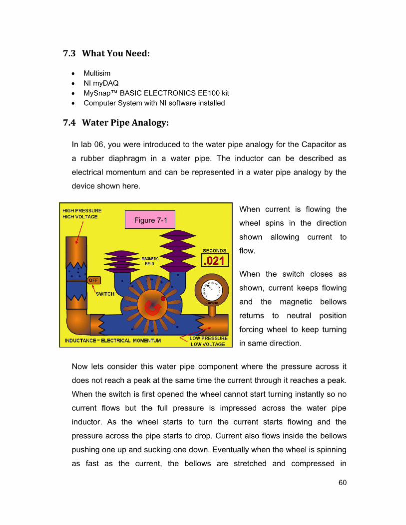
device shown here.

When current is flowing the

wheel spins in the direction

shown allowing current to

flow.

When the switch closes as

shown, current keeps flowing

and the magnetic bellows

returns to neutral position

forcing wheel to keep turning

in same direction.

Now lets consider this water pipe component where the pressure across it

does not reach a peak at the same time the current through it reaches a peak.

When the switch is first opened the wheel cannot start turning instantly so no

current flows but the full pressure is impressed across the water pipe

inductor. As the wheel starts to turn the current starts flowing and the

pressure across the pipe starts to drop. Current also flows inside the bellows

pushing one up and sucking one down. Eventually when the wheel is spinning

as fast as the current, the bellows are stretched and compressed in

Figure 7-1

61

proportion to the current flowing, and the pressure across the inductor pipe is

at a minimum. In this device the voltage (pressure) is present before the

current (water) flows or the voltage leads the current. To better see this

relationship, play the animated .gif file called Coil.gif on the disc that came

with the MySnapTM parts. It can be viewed using an animated .gif player such

as “Windows Media Player”, “Windows Picture and Fax Viewer” or

“QuickTime” just to name a few. Points of interest that should be noted in the

analogy are;

Water pressure (voltage) leads the current by 90°.

Direct water flow (DC) passes through the inductor easily after wheel

spins and bellows are charged (magnetic field is established).

When an Inductor stores energy in a magnetic field (offset bellows) a

condition exist to keep current flowing.

Alternating water flow (AC) is blocked by inducter if water (current)

reverses direction before wheel (magnetic field) can start to spin (high

frequency).

It takes time for current in an inductor to start flowing.

Maximum DC current occurs when there is only back pressure from the

wheel due to friction (resistance in inductor).

Peak magnetic field occurs (bellows stretched and compressed) when

current is at maximum.

Size of wheel and weight or mass of wheel can change Inductors

properties.

7.5 In electric circuits:

An electronic inductor consists of a coil of wire usually wound on a magnetic

core. The size and shape of the coil can greatly increase the value of inductance.

The magnetic core can also change the Inductance. The energy (measured in

joules, in SI units) stored by an inductor is equal to the amount of work required

to establish the current flowing through the inductor, and the magnetic field

established. This is given by:

Estored = ½ LI2

Where, L is inductance and I is the current flowing through the inductor.

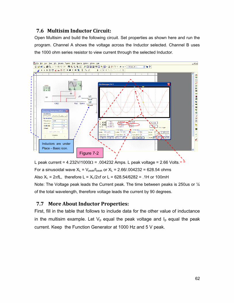
62

7.6 Multisim Inductor Circuit: Open Multisim and build the following circuit. Set properties as shown here and run the

program. Channel A shows the voltage across the Inductor selected. Channel B uses

the 1000 ohm series resistor to view current through the selected Inductor.

L peak current = 4.232V/1000 = .004232 Amps. L peak voltage = 2.66 Volts.

For a sinusoidal wave XL = Vpeak/Ipeak or XL = 2.66/.004232 = 628.54 ohms

Also XL = 2fL, therefore L = XL/2f or L = 628.54/6282 = .1H or 100mH

Note: The Voltage peak leads the Current peak. The time between peaks is 250us or ¼

of the total wavelength, therefore voltage leads the current by 90 degrees.

7.7 More About Inductor Properties:

First, fill in the table that follows to include data for the other value of inductance

in the multisim example. Let Vp equal the peak voltage and Ip equal the peak

current. Keep the Function Generator at 1000 Hz and 5 V peak.

Figure 7-2

Inductors are under

Place – Basic icon.

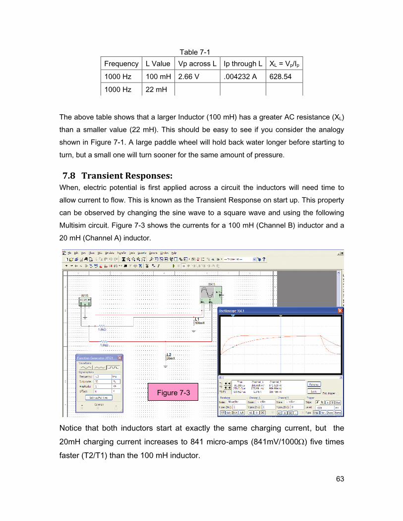
63

The above table shows that a larger Inductor (100 mH) has a greater AC resistance (XL)

than a smaller value (22 mH). This should be easy to see if you consider the analogy

shown in Figure 7-1. A large paddle wheel will hold back water longer before starting to

turn, but a small one will turn sooner for the same amount of pressure.

7.8 Transient Responses: When, electric potential is first applied across a circuit the inductors will need time to

allow current to flow. This is known as the Transient Response on start up. This property

can be observed by changing the sine wave to a square wave and using the following

Multisim circuit. Figure 7-3 shows the currents for a 100 mH (Channel B) inductor and a

20 mH (Channel A) inductor.

Notice that both inductors start at exactly the same charging current, but the

20mH charging current increases to 841 micro-amps (841mV/1000) five times

faster (T2/T1) than the 100 mH inductor.

Frequency L Value Vp across L Ip through L XL = Vp/Ip

1000 Hz 100 mH 2.66 V .004232 A 628.54

1000 Hz 22 mH

Table 7-1

Figure 7-3

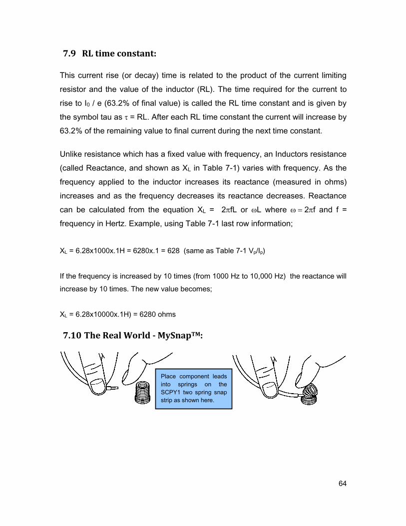
64

7.9 RL time constant:

This current rise (or decay) time is related to the product of the current limiting

resistor and the value of the inductor (RL). The time required for the current to

rise to I0 / e (63.2% of final value) is called the RL time constant and is given by

the symbol tau as = RL. After each RL time constant the current will increase by

63.2% of the remaining value to final current during the next time constant.

Unlike resistance which has a fixed value with frequency, an Inductors resistance

(called Reactance, and shown as XL in Table 7-1) varies with frequency. As the

frequency applied to the inductor increases its reactance (measured in ohms)

increases and as the frequency decreases its reactance decreases. Reactance

can be calculated from the equation XL = 2fL or L where 2f and f =

frequency in Hertz. Example, using Table 7-1 last row information;

XL = 6.28x1000x.1H = 6280x.1 = 628 (same as Table 7-1 Vp/Ip)

If the frequency is increased by 10 times (from 1000 Hz to 10,000 Hz) the reactance will

increase by 10 times. The new value becomes;

XL = 6.28x10000x.1H) = 6280 ohms

7.10 The Real World - MySnapTM:

Place component leads

into springs on the

SCPY1 two spring snap

strip as shown here.

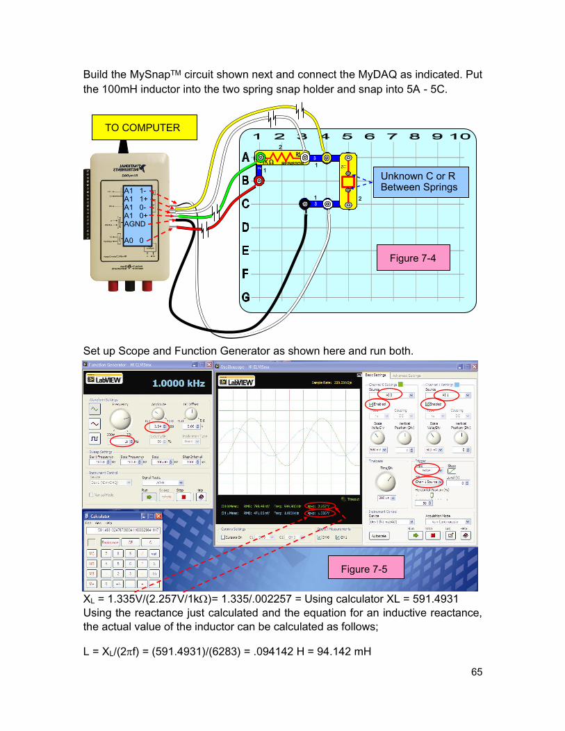
65

TO COMPUTER

Figure 7-4

Unknown C or R Between Springs A1 1-

A1 1+ A1 0- A1 0+ AGND A0 0

1

1

1

2

2

Build the MySnapTM circuit shown next and connect the MyDAQ as indicated. Put

the 100mH inductor into the two spring snap holder and snap into 5A - 5C.

Set up Scope and Function Generator as shown here and run both.

XL = 1.335V/(2.257V/1k)= 1.335/.002257 = Using calculator XL = 591.4931

Using the reactance just calculated and the equation for an inductive reactance,

the actual value of the inductor can be calculated as follows;

L = XL/(2f) = (591.4931)/(6283) = .094142 H = 94.142 mH

Figure 7-5

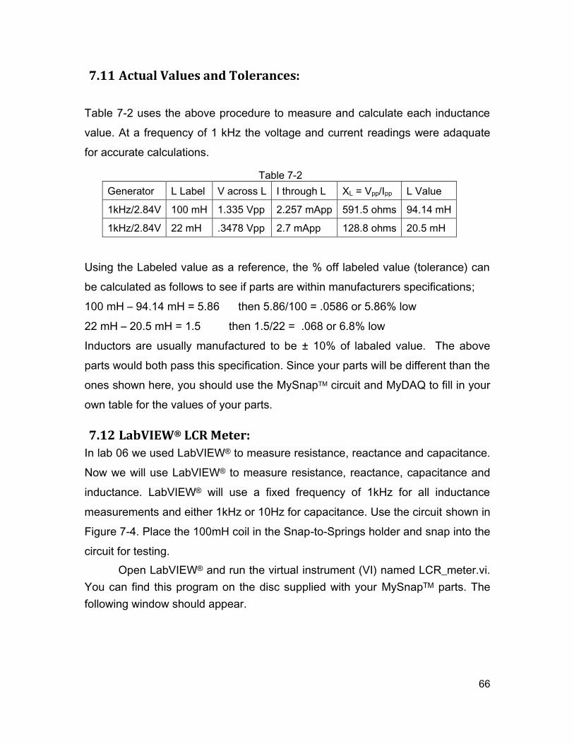
66

7.11 Actual Values and Tolerances:

Table 7-2 uses the above procedure to measure and calculate each inductance

value. At a frequency of 1 kHz the voltage and current readings were adaquate

for accurate calculations.

Generator L Label V across L I through L XL = Vpp/Ipp L Value

1kHz/2.84V 100 mH 1.335 Vpp 2.257 mApp 591.5 ohms 94.14 mH

1kHz/2.84V 22 mH .3478 Vpp 2.7 mApp 128.8 ohms 20.5 mH

Using the Labeled value as a reference, the % off labeled value (tolerance) can

be calculated as follows to see if parts are within manufacturers specifications;

100 mH – 94.14 mH = 5.86 then 5.86/100 = .0586 or 5.86% low

22 mH – 20.5 mH = 1.5 then 1.5/22 = .068 or 6.8% low

Inductors are usually manufactured to be ± 10% of labaled value. The above

parts would both pass this specification. Since your parts will be different than the

ones shown here, you should use the MySnapTM circuit and MyDAQ to fill in your

own table for the values of your parts.

7.12 LabVIEW® LCR Meter:

In lab 06 we used LabVIEW® to measure resistance, reactance and capacitance.

Now we will use LabVIEW® to measure resistance, reactance, capacitance and

inductance. LabVIEW® will use a fixed frequency of 1kHz for all inductance

measurements and either 1kHz or 10Hz for capacitance. Use the circuit shown in

Figure 7-4. Place the 100mH coil in the Snap-to-Springs holder and snap into the

circuit for testing.

Open LabVIEW® and run the virtual instrument (VI) named LCR_meter.vi.

You can find this program on the disc supplied with your MySnapTM parts. The

following window should appear.

Table 7-2

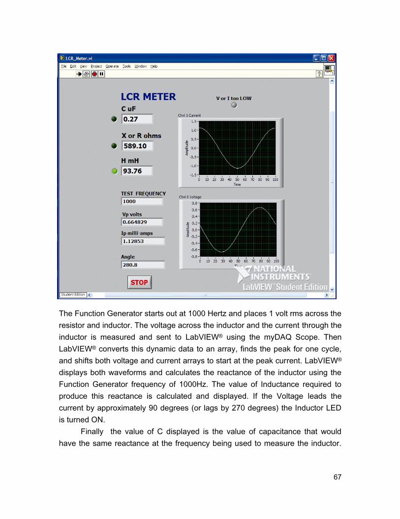
67

The Function Generator starts out at 1000 Hertz and places 1 volt rms across the

resistor and inductor. The voltage across the inductor and the current through the

inductor is measured and sent to LabVIEW® using the myDAQ Scope. Then

LabVIEW® converts this dynamic data to an array, finds the peak for one cycle,

and shifts both voltage and current arrays to start at the peak current. LabVIEW®

displays both waveforms and calculates the reactance of the inductor using the

Function Generator frequency of 1000Hz. The value of Inductance required to

produce this reactance is calculated and displayed. If the Voltage leads the

current by approximately 90 degrees (or lags by 270 degrees) the Inductor LED

is turned ON.

Finally the value of C displayed is the value of capacitance that would

have the same reactance at the frequency being used to measure the inductor.

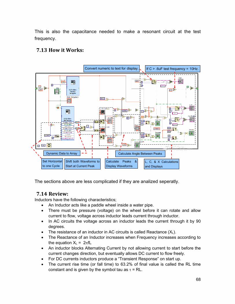
68

This is also the capacitance needed to make a resonant circuit at the test

frequency.

7.13 How it Works:

The sections above are less complicated if they are analized seperatly.

7.14 Review: Inductors have the following characteristics;

An Inductor acts like a paddle wheel inside a water pipe.

There must be pressure (voltage) on the wheel before it can rotate and allow

current to flow, voltage across inductor leads current through inductor.

In AC circuits the voltage across an inductor leads the current through it by 90

degrees.

The resistance of an inductor in AC circuits is called Reactance (XL).

The Reactance of an Inductor increases when Frequency increases according to

the equation XL = 2fL

An inductor blocks Alternating Current by not allowing current to start before the

current changes direction, but eventually allows DC current to flow freely.

For DC currents inductors produce a “Transient Response” on start up.

The current rise time (or fall time) to 63.2% of final value is called the RL time

constant and is given by the symbol tau as = RL.

Convert numeric to text for display.

If C > .6uF test frequency = 10Hz.

Dynamic Data to Array

Set Horizontal

to one Cycle

Shift both Waveforms to

Start at Current Peak

Calculate Peaks &

Display Waveforms

Calculate Angle Between Peaks

L, C, & X Calculations

and Displays

69

Because it takes time to start current flowing in an inductor, the current in an

inductor cannot be changed instantly as for a resistor.

LabVIEW® LCR meter shows phase angle between current and voltage for

components being measured.

LabVIEW® LCR meter uses a components characteristics to calculate the type of

component being tested, its values at a given frequency, and display results.

70

Lab 08: The Diode

The Diode is an electrical device characterized by its capacity to conduct current

in one direction and block current flow in the opposite direction. This lab will

explain the diode using a water pipe analogy, virtual diodes using Multisim, real

diodes using MySnapTM and the diode curve tracer virtual instrument called

DIODE.VI. This VI can be found in ENGR190_Vis.zip file. In the real world,

measurements will be taken with the myDAQ DMM and then displayed on the

diode curve tracer. The components to be measured are supplied in the

MySnap™ model “BASIC ELECTRONICS EE100”. Real life applications apply to

anything that converts AC to DC or detects and demodulates signals, such as

power supplies, radios, and television just to name a few.


Objective

What you need

Water pipe analogy

In electronic circuits

Multisim diode circuit

AC to DC conversion

More about diode properties

The real world diode

Diode (D1) measured parameters

Diode equation

Review

8.2 Objective:


and AC properties of diodes in electronic circuits. Study diode responses and

relationship between current and voltage using a diode curve tracer.

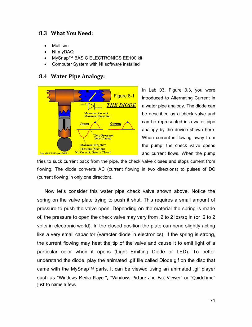
71

8.3 What You Need:

Multisim

NI myDAQ




In Lab 03, Figure 3.3, you were

introduced to Alternating Current in

a water pipe analogy. The diode can

be described as a check valve and

can be represented in a water pipe

analogy by the device shown here.

When current is flowing away from

the pump, the check valve opens

and current flows. When the pump

tries to suck current back from the pipe, the check valve closes and stops current from

flowing. The diode converts AC (current flowing in two directions) to pulses of DC

(current flowing in only one direction).

Now let’s consider this water pipe check valve shown above. Notice the

spring on the valve plate trying to push it shut. This requires a small amount of

pressure to push the valve open. Depending on the material the spring is made

of, the pressure to open the check valve may vary from .2 to 2 lbs/sq in (or .2 to 2

volts in electronic world). In the closed position the plate can bend slightly acting

like a very small capacitor (varacter diode in electronics). If the spring is strong,

the current flowing may heat the tip of the valve and cause it to emit light of a

particular color when it opens (Light Emitting Diode or LED). To better

understand the diode, play the animated .gif file called Diode.gif on the disc that

came with the MySnapTM parts. It can be viewed using an animated .gif player

such as “Windows Media Player”, “Windows Picture and Fax Viewer” or “QuickTime”

just to name a few.

Figure 8-1

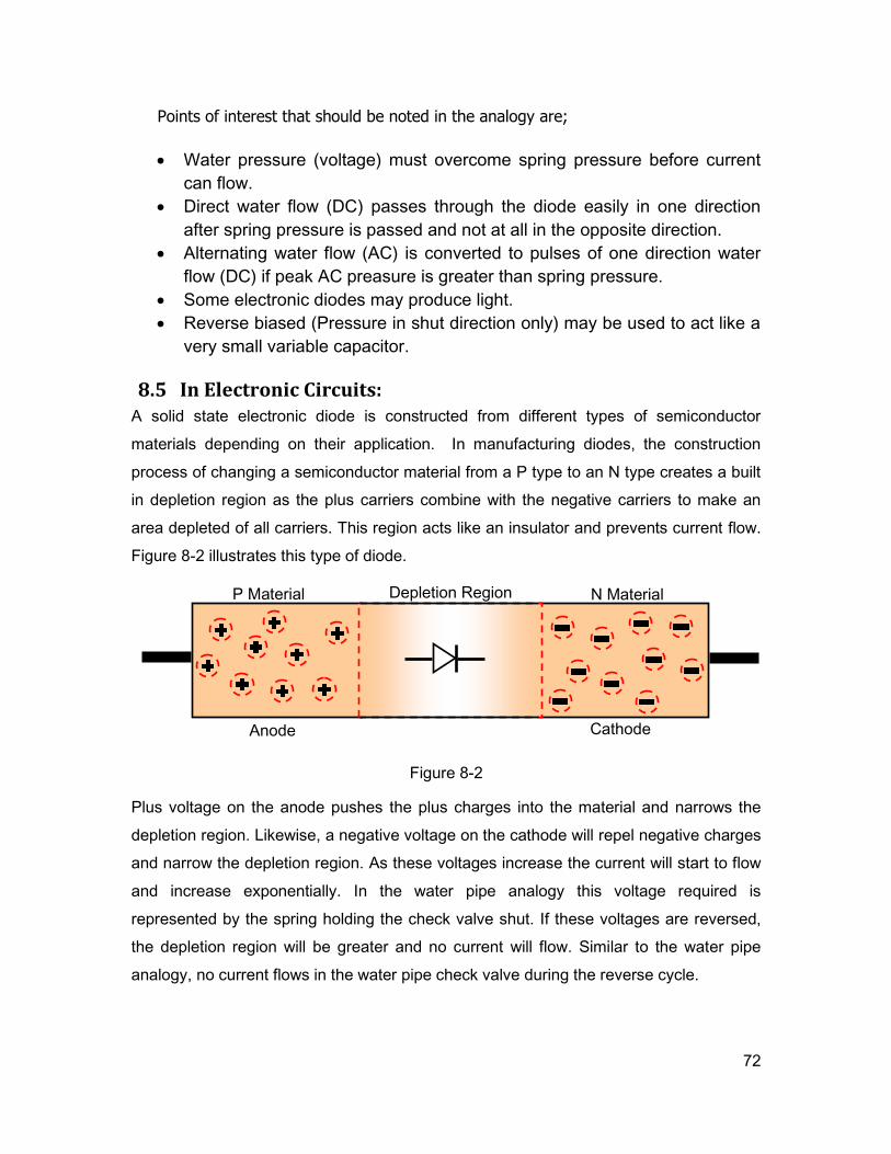
72

Points of interest that should be noted in the analogy are;

Water pressure (voltage) must overcome spring pressure before current

can flow.

Direct water flow (DC) passes through the diode easily in one direction

after spring pressure is passed and not at all in the opposite direction.

Alternating water flow (AC) is converted to pulses of one direction water

flow (DC) if peak AC preasure is greater than spring pressure.

Some electronic diodes may produce light.

Reverse biased (Pressure in shut direction only) may be used to act like a

very small variable capacitor.

8.5 In Electronic Circuits: A solid state electronic diode is constructed from different types of semiconductor

materials depending on their application. In manufacturing diodes, the construction

process of changing a semiconductor material from a P type to an N type creates a built

in depletion region as the plus carriers combine with the negative carriers to make an

area depleted of all carriers. This region acts like an insulator and prevents current flow.

Figure 8-2 illustrates this type of diode.

Plus voltage on the anode pushes the plus charges into the material and narrows the

depletion region. Likewise, a negative voltage on the cathode will repel negative charges

and narrow the depletion region. As these voltages increase the current will start to flow

and increase exponentially. In the water pipe analogy this voltage required is

represented by the spring holding the check valve shut. If these voltages are reversed,

the depletion region will be greater and no current will flow. Similar to the water pipe

analogy, no current flows in the water pipe check valve during the reverse cycle.

Figure 8-2

P Material N Material Depletion Region

Anode Cathode

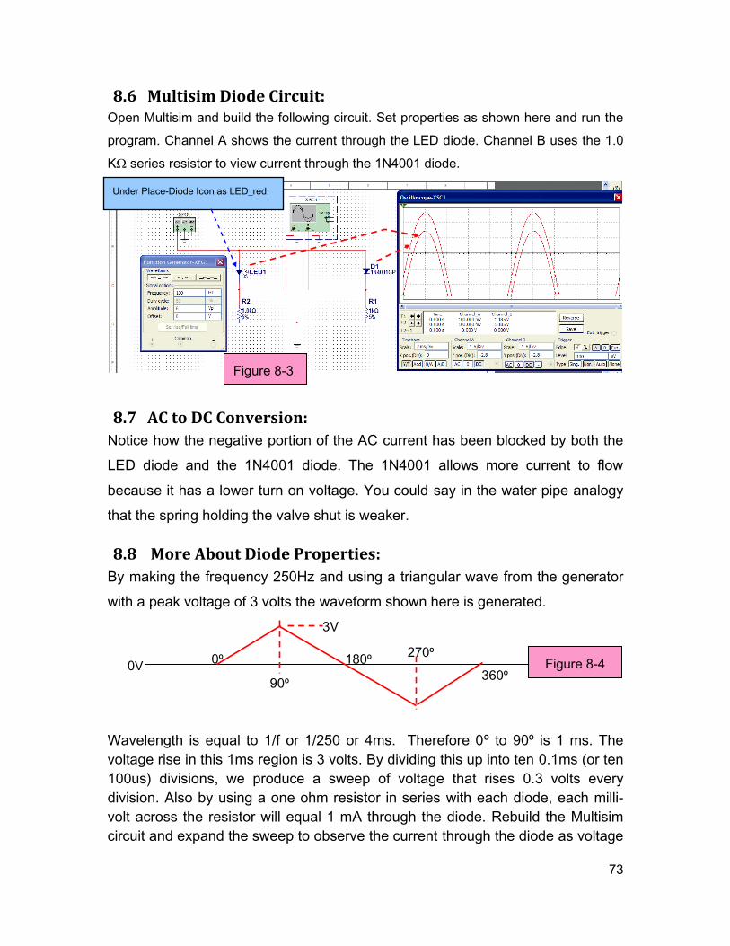
73

8.6 Multisim Diode Circuit: Open Multisim and build the following circuit. Set properties as shown here and run the

program. Channel A shows the current through the LED diode. Channel B uses the 1.0

KΩ series resistor to view current through the 1N4001 diode.

8.7 AC to DC Conversion:

Notice how the negative portion of the AC current has been blocked by both the

LED diode and the 1N4001 diode. The 1N4001 allows more current to flow

because it has a lower turn on voltage. You could say in the water pipe analogy

that the spring holding the valve shut is weaker.

8.8 More About Diode Properties:

By making the frequency 250Hz and using a triangular wave from the generator

with a peak voltage of 3 volts the waveform shown here is generated.

Wavelength is equal to 1/f or 1/250 or 4ms. Therefore 0º to 90º is 1 ms. The

voltage rise in this 1ms region is 3 volts. By dividing this up into ten 0.1ms (or ten

100us) divisions, we produce a sweep of voltage that rises 0.3 volts every

division. Also by using a one ohm resistor in series with each diode, each milli-

volt across the resistor will equal 1 mA through the diode. Rebuild the Multisim

circuit and expand the sweep to observe the current through the diode as voltage

Figure 8-3

0º

90º

180º

270º

360º

3V

0V

Figure 8-4

Under Place-Diode Icon as LED_red.

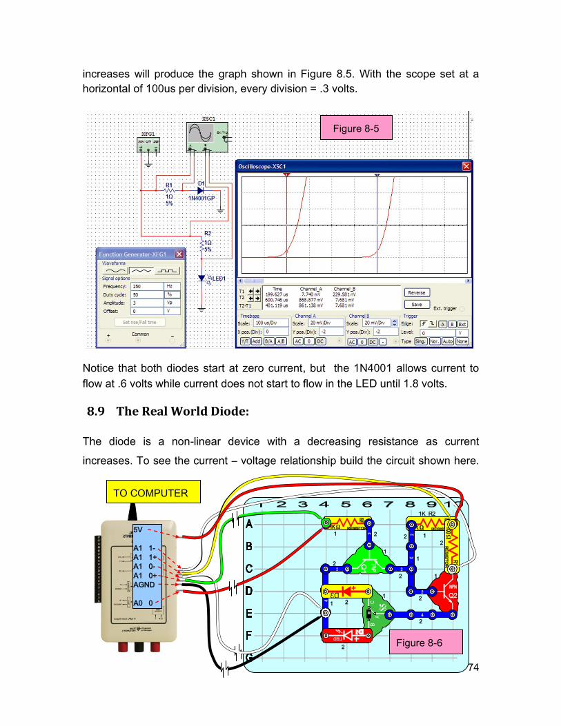
74

increases will produce the graph shown in Figure 8.5. With the scope set at a

horizontal of 100us per division, every division = .3 volts.

Notice that both diodes start at zero current, but the 1N4001 allows current to

flow at .6 volts while current does not start to flow in the LED until 1.8 volts.

8.9 The Real World Diode:

The diode is a non-linear device with a decreasing resistance as current

increases. To see the current – voltage relationship build the circuit shown here.

Figure 8-5

TO COMPUTER

Figure 8-6

5V

A1 1-

A1 1+

A1 0-

A1 0+

AGND

A0 0

1 1

1

1

1

1

1 2

2

2

2

2

2 2

2

2

1K R2

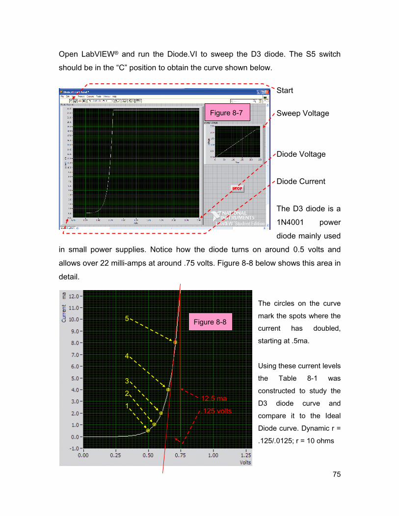
75

Figure 8-7

5

4

3

2

1 12.5 ma

.125 volts

Figure 8-8

Open LabVIEW® and run the Diode.VI to sweep the D3 diode. The S5 switch

should be in the “C” position to obtain the curve shown below.

Start

Sweep Voltage

Diode Voltage

Diode Current

The D3 diode is a

1N4001 power

diode mainly used

in small power supplies. Notice how the diode turns on around 0.5 volts and

allows over 22 milli-amps at around .75 volts. Figure 8-8 below shows this area in

detail.

The circles on the curve

mark the spots where the

current has doubled,

starting at .5ma.

Using these current levels

the Table 8-1 was

constructed to study the

D3 diode curve and

compare it to the Ideal

Diode curve. Dynamic r =

.125/.0125; r = 10 ohms

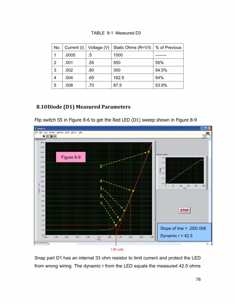
76

8.10 Diode (D1) Measured Parameters

Flip switch S5 in Figure 8-6 to get the Red LED (D1) sweep shown in Figure 8-9

Snap part D1 has an internal 33 ohm resistor to limit current and protect the LED

from wrong wiring. The dynamic r from the LED equals the measured 42.5 ohms

No. Current (I) Voltage (V) Static Ohms (R=V/I) % of Previous

1 .0005 .5 1000 --------

2 .001 .55 550 55%

3 .002 .60 300 54.5%

4 .004 .65 162.5 54%

5 .008 .70 87.5 53.9%

TABLE 8-1 Measured D3

Parameters

Figure 8-9

1.65 volts

5

4

3

2

1

Slope of line = .255/.006

Dynamic r = 42.5

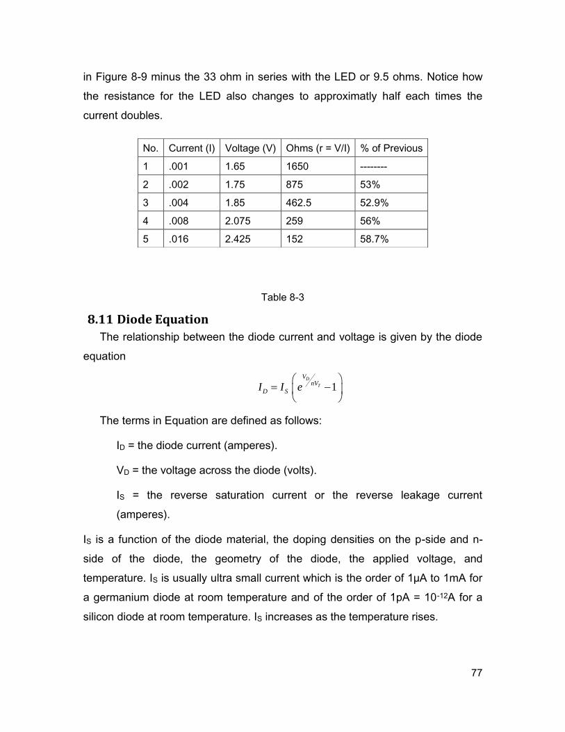
77

in Figure 8-9 minus the 33 ohm in series with the LED or 9.5 ohms. Notice how

the resistance for the LED also changes to approximatly half each times the

current doubles.

8.11 Diode Equation

The relationship between the diode current and voltage is given by the diode

equation

1D

T

VnV

D SI I e

The terms in Equation are defined as follows:

ID = the diode current (amperes).

VD = the voltage across the diode (volts).

IS = the reverse saturation current or the reverse leakage current

(amperes).

IS is a function of the diode material, the doping densities on the p-side and n-

side of the diode, the geometry of the diode, the applied voltage, and

temperature. IS is usually ultra small current which is the order of 1μA to 1mA for

a germanium diode at room temperature and of the order of 1pA = 10-12A for a

silicon diode at room temperature. IS increases as the temperature rises.

No. Current (I) Voltage (V) Ohms (r = V/I) % of Previous

1 .001 1.65 1650 --------

2 .002 1.75 875 53%

3 .004 1.85 462.5 52.9%

4 .008 2.075 259 56%

5 .016 2.425 152 58.7%

Table 8-3

78

VT = kT/q = the thermal equivalent voltage = 0.0258 V at room

temperature

where

q = 1.6 x 10-19 Coulombs = the electric charge,

k = 1.38 x 10-23 J/K = Boltzmann's constant,

and

T = absolute temperature (Kelvin) [room temperature = 300 K].

n = the ideality factor or the emission coefficient.

8.12 Review:

Diodes have the following characteristics;

A Diode acts like a check valve inside a water pipe.

There must be forward pressure (voltage) on the check valve before it can

open and allow current to flow, no current will flow if voltage across diode

is less than the threshold voltage.

In AC circuits the diode will convert alternating current into pulses of direct

current.

The resistance of a diode is nonlinear and changes with current.

A reverse biased diode can act as a very small capacitor.

Voltage and current in a diode are in phase, no phase shift.

Diode turn on voltages can vary depending on materials and type of diode.

Some diodes can produce light when current flows.

LabVIEW® Diode.VI shows diode current when a forward sweep voltage is

applied.

79

Appendix A: Basic Definitions and Conventions AC

Alternating current. Consists of a periodic oscillation between two different voltages.

Usually said to look like a sine wave, but is not always.

Ampere (A)

The SI unit for the electrical current. An Ampere of current flow represents electron

movement at a rate of one coulomb per second: that amount of current through one ohm

of resistance with one volt applied.

Amplify

To increase the strength of the signal.

Anode

An electron collector. An anode has a more positive voltage relative to a cathode.

Attenuate

Decrease the strength of a signal.

Capacitor

An electronics component that stores energy in the form of electric charge (static

electricity). It resists a sudden change in voltage.

Cathode

An electron emitter. A cathode has a more negative voltage relative to an anode.

Charge

Particles can have two possible types of charge: positive or negative. Electrons are

negatively charged, protons are positively charged. Opposite charges attract, while

particles with the same charge (either positive or negative) repel each other.

Choke

Another name for an inductor, specifically referring to those used in power regulation.

Circuit

The paths electrons take as they are pushed by some power source, flow through various

electrical components then return to the power source.

Short Circuit exist, when there is no resistance between two points. Current flows without

a change in voltage.

Open Circuit exist when there is infinite resistance between two points. Current is unable

to flow, but there is still a voltage between the two points.

Coil

A helix of wire. Its height, width, thickness, and material can all vary. Often used as an

inductor.

Condenser

Another name for capacitor.

Conductance

The inverse of resistance. Measured in siemens (obsolete name mhos), which are the

inverse of ohms. 1 S = 1/Ω = 1 A/V

Conductor:

A material that has many free electrons.

Coulomb (C)

The SI unit for electric charge Q. Defined in terms of the ampere. 1 coulomb is the

amount of electric charge carried by a current of 1 ampere flowing for 1 second. It is also

about 6.24×1018 times the charge on an electron. 1 C = 1 A·s

Current

The movement of charges in an electric field. This is perceived as a flow. It is measured

in amperes.

80

Cycles per second (cps)

An obsolete name for Hertz, the standard SI unit for frequency. As the name implies, a

measurement of frequency in full cycles of a wave per second.

DC

Direct current. A constant voltage and a constant current flow in one direction.

Diode

A one way valve for current. Semiconductor diodes typically have a voltage drop of 0.6 V

(silicon) or 0.2V (germanium) when conducting in the forward direction.

Electron:

The negatively charged particle in an atom orbiting the atom's nucleus.

EMF (E)

Electro-Motive Force. A force for moving electrons. See Voltage.

Farad (F)

The SI unit for capacitance (C). A capacitor has a capacitance of 1

Farad when a charge of 1 Coulomb raises its potential 1 Volt.

Forward Biased

The voltage polarity through a part which causes it to conduct current.

Farad:

Unit of measurement of capacitance. A capacitor has a capacitance of 1 Farad when a charge of 1 Coulomb raises its potential 1 Volt.

Frequency (f) Number of times a periodic waveform repeats itself in a unit time (generally seconds).

Units of measurement are Hertz.

Gain

A multiplier of voltage or current.

Ground

Ground is defined as the point in the circuit which is at zero voltage. Voltage is relative,

and is the same throughout a conductor, so any point in the circuit can be defined as

ground, and all other voltages are referenced to it. Usually it is defined as the most

negative point in the circuit, for convenience. Sometimes it is defined in the middle of two

bi-polar rails, for "balanced" circuits. In many cases this circuit point is connected to the

Earth (Ground) by a conductor.

Henry (H)

The SI unit for inductance. A coil has 1 Henry of inductance if an emf of 1 Volt is induced

when current through the inductor is changing at a rate of 1 Ampere per second.

Hertz (Hz)

The SI unit for frequency. One Hz is one cycle per second.

Impedance

A more generalized form of resistance. The impedance of a device varies with the

frequency of the electricity applied. A perfect resistor will have a constant impedance for

all frequencies. Capacitors and inductors have varying impedances at different

frequencies. Measured in ohms or Ω.

Inductor

An inductor is a device that stores energy in a magnetic field. It opposes a sudden

change in the flow of current. Units of measurement are Henrys.

Kirchhoff's Current Law:

At any junction of conductors in a circuit, the algebraic sum of currents is zero.

Kirchhoff's Voltage Law:

The algebraic sum of voltages around a circuit is zero.

Length (l) A measure of distance usually in meters (m).

81

Load:

Resistance connected across a circuit that determines power used.

Meter (m)

The SI unit for distance. The distance light travels in 1/299,792,458 second.

Ohm (Ω)

The basic unit of resistance or impedance: the amount of electrical resistance limiting the

current to one ampere with one volt applied.

Ohm's Law:

Mathematical relationship between current, voltage and resistance stating that when a

voltage is applied to a conductor, the current moving through the conductor is proportional to the applied voltage. Discovered by Georg Simon Ohm. (Name spelled correctly)

Op-amp

Short for operational amplifier. An op-amp amplifies the voltage between its two inputs.

Parallel:

Used to describe two or more circuits or circuit elements so connected that the total

current flow is divided between them.

PCB

Printed circuit board. This is a piece of plastic or fiberglass with copper attached. The

copper is typically chemically etched away to leave "traces" for the electricity to be

conducted through. Other electrical components are soldered to the traces.

Period

The time between cycles of a periodic wave.

Power

Voltage times current. The amount of work being done by a circuit.

Rectify

Convert AC current to DC current.

Reactance

Opposition to ac as a result of inductance or capacitance.

Resistance Properties of a circuit that impede the flow of electrons. Resistance converts electrical energy into photons that are given off as waste heat. Resistance is measured in ohms.

Reversed Biased

The inverted voltage polarity on a part.

Root-Mean Squared (RMS)

The effective DC value for an AC value.

Second (s)

The SI unit for time.

Series Circuit:

A circuit that contains only one possible path for electron flow supplied by a common voltage source.

SI

The standard system of units.

Time (t)

The symbol for time in seconds (s).

Transistor A device in which the resistance of the channel is controlled by a current or voltage at the base or gate. Can be thought of as an electronic-controlled resistor.

Volt (V)

A potential due to an electric field. One volt is defined as the potential difference across a

resistor that is passing one ampere and dissipating one watt. 1 V = 1 W/A

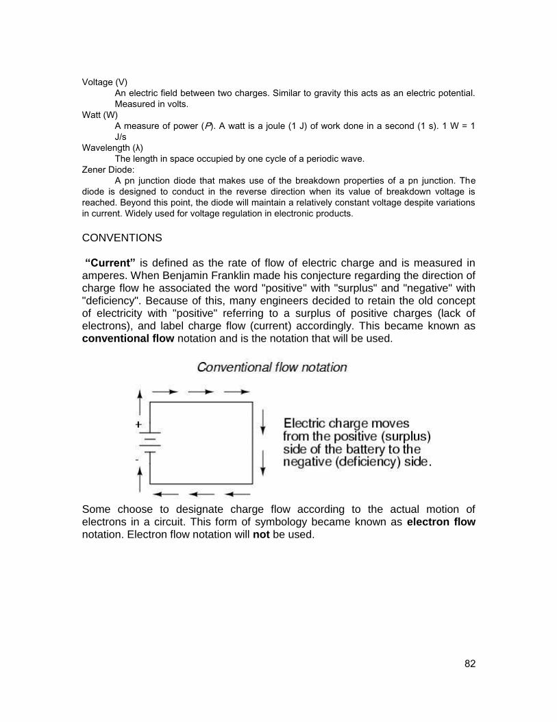
82

Voltage (V)

An electric field between two charges. Similar to gravity this acts as an electric potential.

Measured in volts.

Watt (W)

A measure of power (P). A watt is a joule (1 J) of work done in a second (1 s). 1 W = 1

J/s

Wavelength (λ)

The length in space occupied by one cycle of a periodic wave.

Zener Diode:

A pn junction diode that makes use of the breakdown properties of a pn junction. The

diode is designed to conduct in the reverse direction when its value of breakdown voltage is

reached. Beyond this point, the diode will maintain a relatively constant voltage despite variations

in current. Widely used for voltage regulation in electronic products.

CONVENTIONS “Current” is defined as the rate of flow of electric charge and is measured in amperes. When Benjamin Franklin made his conjecture regarding the direction of charge flow he associated the word "positive" with "surplus" and "negative" with "deficiency". Because of this, many engineers decided to retain the old concept of electricity with "positive" referring to a surplus of positive charges (lack of electrons), and label charge flow (current) accordingly. This became known as conventional flow notation and is the notation that will be used.

Some choose to designate charge flow according to the actual motion of electrons in a circuit. This form of symbology became known as electron flow notation. Electron flow notation will not be used.

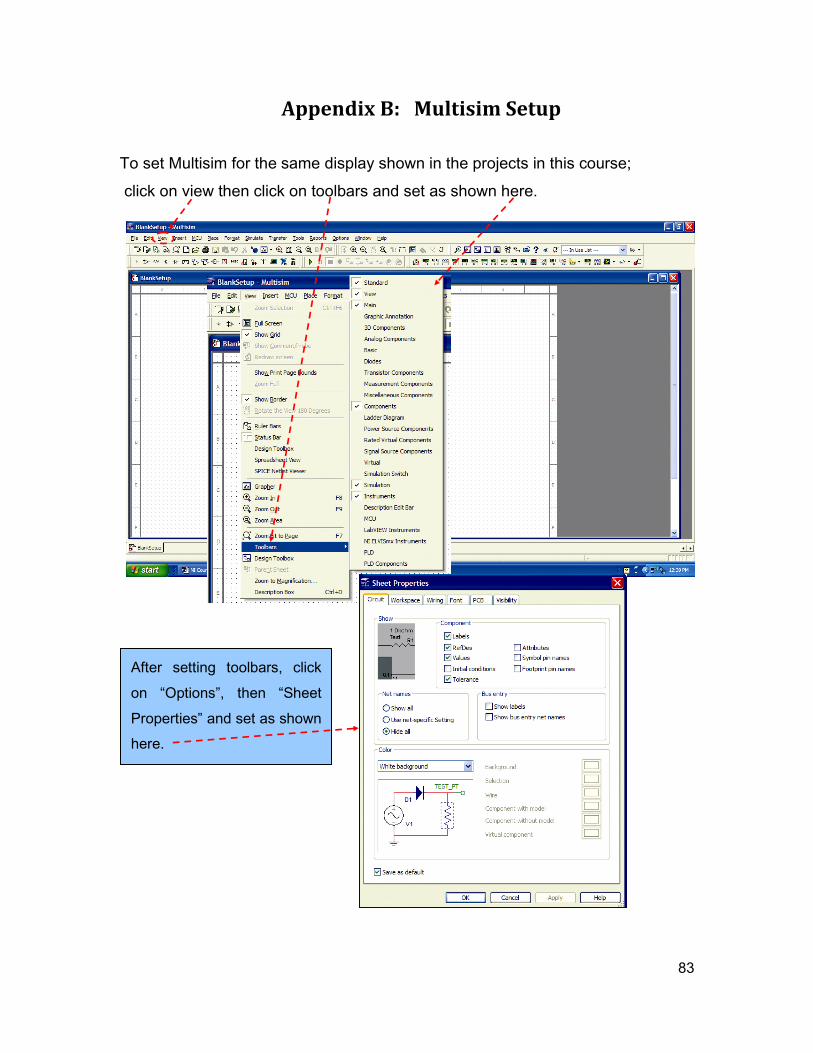
83

Appendix B: Multisim Setup

To set Multisim for the same display shown in the projects in this course;

click on view then click on toolbars and set as shown here.

After setting toolbars, click

on “Options”, then “Sheet

Properties” and set as shown

here.

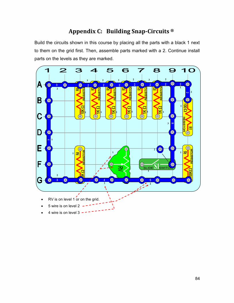
84

1

1 1 1 1 1 1

1

1

1

1

1

2

2 2

1

2 3 3 3

3

2

2 3

2

2

Appendix C: Building Snap-Circuits ®

Build the circuits shown in this course by placing all the parts with a black 1 next

to them on the grid first. Then, assemble parts marked with a 2. Continue install

parts on the levels as they are marked.

RV is on level 1 or on the grid.

5 wire is on level 2

4 wire is on level 3

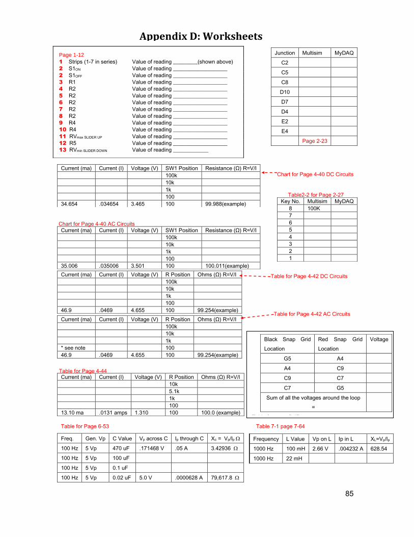
85

Appendix D: Worksheets

Chart for Page 4-40 DC Circuits

Table for Page 4-42 DC Circuits

Table for Page 4-42 AC Circuits

Table for Page 6-53 Table 7-1 page 7-64

Junction Multisim MyDAQ

C2

C5

C8

D10

D7

D4

E2

E4

Page 2-23

Page 1-12

1 Strips (1-7 in series) Value of reading _________(shown above)

2 S1ON Value of reading ____________________

2 S1OFF Value of reading ____________________









11 RVmax SLIDER UP Value of reading ____________________


13 RVmin SLIDER DOWN Value of reading _____________


100k

10k

1k

100

35.006 .035006 3.501 100 100.011(example)


100k

10k

1k

100

34.654 .034654 3.465 100 99.988(example) Key No. Multisim MyDAQ

8 100K

7

6

5

4

3

2

1


100k

10k

1k

100

46.9 .0469 4.655 100 99.254(example)


100k

10k

1k

* see note 100

46.9 .0469 4.655 100 99.254(example)


10k

5.1k

1k

100

13.10 ma .0131 amps 1.310 100 100.0 (example)

Freq. Gen. Vp C Value Vp across C Ip through C Xc = Vp/Ip

100 Hz 5 Vp 470 uF .171468 V .05 A 3.42936

100 Hz 5 Vp 100 uF

100 Hz 5 Vp 0.1 uF

100 Hz 5 Vp 0.02 uF 5.0 V .0000628 A 79,617.8

Black Snap Grid

Location

Red Snap Grid

Location

Voltage

G5 A4

A4 C9

C9 C7

C7 G5

Sum of all the voltages around the loop

=

Table for page 5-47

WORKSHEET PAGE

Chart for Page 4-40 AC Circuits

Table for Page 4-44

Table2-2 for Page 2-27

Frequency L Value Vp on L Ip in L XL=Vp/Ip

1000 Hz 100 mH 2.66 V .004232 A 628.54

1000 Hz 22 mH

creative inquiry electronics project lab manual inquiry electronics project lab manual ni mydaq

Documents