creating relational data from unstructured and ...journal of artificial intelligence research 31...
TRANSCRIPT

Journal of Artificial Intelligence Research 31 (2008) 543-590 Submitted 08/07; published 03/08
Creating Relational Data from Unstructured andUngrammatical Data Sources
Matthew Michelson [email protected]
Craig A. Knoblock [email protected]
University of Southern CaliforniaInformation Sciences Instistute4676 Admiralty WayMarina del Rey, CA 90292 USA
Abstract
In order for agents to act on behalf of users, they will have to retrieve and integratevast amounts of textual data on the World Wide Web. However, much of the useful dataon the Web is neither grammatical nor formally structured, making querying difficult.Examples of these types of data sources are online classifieds like Craigslist1 and auctionitem listings like eBay.2 We call this unstructured, ungrammatical data “posts.” Theunstructured nature of posts makes query and integration difficult because the attributesare embedded within the text. Also, these attributes do not conform to standardized values,which prevents queries based on a common attribute value. The schema is unknown andthe values may vary dramatically making accurate search difficult. Creating relationaldata for easy querying requires that we define a schema for the embedded attributes andextract values from the posts while standardizing these values. Traditional informationextraction (IE) is inadequate to perform this task because it relies on clues from the data,such as structure or natural language, neither of which are found in posts. Furthermore,traditional information extraction does not incorporate data cleaning, which is necessary toaccurately query and integrate the source. The two-step approach described in this papercreates relational data sets from unstructured and ungrammatical text by addressing bothissues. To do this, we require a set of known entities called a “reference set.” The first stepaligns each post to each member of each reference set. This allows our algorithm to define aschema over the post and include standard values for the attributes defined by this schema.The second step performs information extraction for the attributes, including attributes noteasily represented by reference sets, such as a price. In this manner we create a relationalstructure over previously unstructured data, supporting deep and accurate queries over thedata as well as standard values for integration. Our experimental results show that ourtechnique matches the posts to the reference set accurately and efficiently and outperformsstate-of-the-art extraction systems on the extraction task from posts.
1. Introduction
The future vision of the Web includes computer agents searching for information, makingdecisions and taking actions on behalf of human users. For instance, an agent could querya number of data sources to find the lowest price for a given car and then email the userthe car listing, along with directions to the seller and available appointments to see the car.
1. www.craigslist.org2. www.ebay.com
c©2008 AI Access Foundation. All rights reserved.
Michelson & Knoblock
This requires the agent to contain two data gathering mechanisms: the ability to querysources and the ability to integrate relevant sources of information.
However, these data gathering mechanisms assume that the sources themselves are de-signed to support relational queries, such as having well defined schema and standard valuesfor the attributes. Yet this is not always the case. There are many data sources on theWorld Wide Web that would be useful to query, but the textual data within them is un-structured and is not designed to support querying. We call the text of such data sources“posts.” Examples of “posts” include the text of eBay auction listings, Internet classifiedslike Craigslist, bulletin boards such as Bidding For Travel3, or even the summary text belowthe hyperlinks returned after querying Google. As a running example, consider the threeposts for used car classifieds shown in Table 1.
Table 1: Three posts for Honda Civics from CraigslistCraigslist Post93 civic 5speed runs great obo (ri) $180093- 4dr Honda Civc LX Stick Shift $180094 DEL SOL Si Vtec (Glendale) $3000
The current method to query posts, whether by an agent or a person, is keyword search.However, keyword search is inaccurate and cannot support relational queries. For example,a difference in spelling between the keyword and that same attribute within a post wouldlimit that post from being returned in the search. This would be the case if a user searchedthe example listings for “Civic” since the second post would not be returned. Another factorwhich limits keyword accuracy is the exclusion of redundant attributes. For example, someclassified posts about cars only include the car model, and not the make, since the make isimplied by the model. This is shown in the first and third post of Table 1. In these cases,if a user does a keyword search using the make “Honda,” these posts will not be returned.
Moreover, keyword search is not a rich query framework. For instance, consider thequery, What is the average price for all Hondas from 1999 or later? To do this withkeyword search requires a user to search on “Honda” and retrieve all that are from 1999or later. Then the user must traverse the returned set, keeping track of the prices andremoving incorrectly returned posts.
However, if a schema with standardized attribute values is defined over the entities inthe posts, then a user could run the example query using a simple SQL statement anddo so accurately, addressing both problems created by keyword search. The standardizedattribute values ensure invariance to issues such as spelling differences. Also, each post isassociated with a full schema with values, so even though a post might not contain a carmake, for instance, its schema does and has the correct value for it, so it will be returnedin a query on car makes. Furthermore, these standardized values allow for integration ofthe source with outside sources. Integrating sources usually entails joining the two sourcesdirectly on attributes or translations of the attributes. Without standardized values and
3. www.biddingfortravel.com
544
Relational Data from Unstructured Data Sources
a schema, it would not be possible to link these ungrammatical and unstructured datasources with outside sources. This paper addresses the problem of adding a schema withstandardized attributes over the set of posts, creating a relational data set that can supportdeep and accurate queries.
One way to create a relational data set from the posts is to define a schema andthen fill in values for the schema elements using techniques such as information extrac-tion. This is sometimes called semantic annotation. For example, taking the secondpost of Table 1 and semantically annotating it might yield “93- 4dr Honda Civc LX StickShift $1800 <make>Honda< \make> <model>Civc< \model> <trim>4dr LX< \trim><year>1993< \year> <price>1800< \price>.” However, traditional information extrac-tion, relies on grammatical and structural characteristics of the text to identify the attributesto extract. Yet posts by definition are not structured or grammatical. Therefore, wrapperextraction technologies such as Stalker (Muslea, Minton, & Knoblock, 2001) or RoadRunner(Crescenzi, Mecca, & Merialdo, 2001) cannot exploit the structure of the posts. Nor areposts grammatical enough to exploit Natural Language Processing (NLP) based extractiontechniques such as those used in Whisk (Soderland, 1999) or Rapier (Califf & Mooney,1999).
Beyond the difficulties in extracting the attributes within a post using traditional ex-traction methods, we also require that the values for the attributes are standardized, whichis a process known as data cleaning. Otherwise, querying our newly relational data wouldbe inaccurate and boil down to keyword search. For instance, using the annotation above,we would still need to query where the model is “Civc” to return this record. Traditionalextraction does not address this.
However, most data cleaning algorithms assume that there are tuple-to-tuple transfor-mations (Lee, Ling, Lu, & Ko, 1999; Chaudhuri, Ganjam, Ganti, & Motwani, 2003). Thatis, there is some function that maps the attributes of one tuple to the attributes of an-other. This approach would not work on ungrammatical and unstructured data, where allthe attributes are embedded within the post, which maps to a set of attributes from thereference set. Therefore we need to take a different approach to the problems of figuringout the attributes within a post and cleaning them.
Our approach to creating relational data sets from unstructured and ungrammaticalposts exploits “reference sets.” A reference set consists of collections of known entitieswith the associated, common attributes. A reference set can be an online (or offline) setof reference documents, such as the CIA World Fact Book.4 It can also be an online (oroffline) database, such as the Comics Price Guide.5 With the Semantic Web one can envisionbuilding reference sets from the numerous ontologies that already exist. Using standardizedontologies to build reference sets allows a consensus agreement upon reference set values,which implies higher reliability for these reference sets over others that might exist as oneexpert’s opinion. Using our car example, a reference set might be the Edmunds car buyingguide6, which defines a schema for cars as well as standard values for attributes such asthe model and the trim. In order to construct reference sets from Web sources, such as the
4. http://www.cia.gov/cia/publications/factbook/5. www.comicspriceguide.com6. www.edmunds.com
545

Michelson & Knoblock
Edmunds car buying guide, we use wrapper technologies (Agent Builder7 in this case) toscrape data from the Web source, using the schema that the source defines for the car.
To use a reference set to build a relational data set we exploit the attributes in thereference set to determine the attributes from the post that can be extracted. The first stepof our algorithm finds the best matching member of the reference set for the post. This iscalled the “record linkage” step. By matching a post to a member of the reference set wecan define schema elements for the post using the schema of the reference set, and we canprovide standard attributes for these attributes by using the attributes from the referenceset when a user queries the posts.
Next, we perform information extraction to extract the actual values in the post thatmatch the schema elements defined by the reference set. This step is the informationextraction step. During the information extraction step, the parts of the post are extractedthat best match the attribute values from the reference set member chosen during therecord linkage step. In this step we also extract attributes that are not easily representedby reference sets, such as prices or dates. Although we already have the schema andstandardized attributes required to create a relational data set over the posts, we stillextract the actual attributes embedded within the post so that we can more accuratelylearn to extract the attributes not represented by a reference set, such as prices and dates.While these attributes can be extracted using regular expressions, if we extract the actualattributes within the post we might be able to do so more accurately. For example, considerthe “Ford 500” car. Without actually extracting the attributes within a post, we mightextract “500” as a price, when it is actually a car name. Our overall approach is outlinedin Figure 1.
Although we previously describe a similar approach to semantically annotating posts(Michelson & Knoblock, 2005), this paper extends that research by combining the annota-tion with our work on more scalable record matching (Michelson & Knoblock, 2006). Notonly does this make the matching step for our annotation more scalable, it also demonstratesthat our work on efficient record matching extends to our unique problem of matching posts,with embedded attributes, to structured, relational data. This paper also presents a moredetailed description than our past work, including a more thorough evaluation of the pro-cedure than previously, using larger experimental data sets including a reference set thatincludes tens of thousands of records.
This article is organized as follows. We first describe our algorithm for aligning theposts to the best matching members of the reference set in Section 2. In particular, weshow how this matching takes place, and how we efficiently generate candidate matchesto make the matching procedure more scalable. In Section 3, we demonstrate how toexploit the matches to extract the attributes embedded within the post. We present someexperiments in Section 4, validating our approaches to blocking, matching and informationextraction for unstructured and ungrammatical text. We follow with a discussion of theseresults in Section 5 and then present related work in Section 6. We finish with some finalthoughts and conclusions in Section 7.
7. A product of Fetch Technologies http://www.fetch.com/products.asp
546

Relational Data from Unstructured Data Sources
Figure 1: Creating relational data from unstructured sources
2. Aligning Posts to a Reference Set
To exploit the reference set attributes to create relational data from the posts, the algo-rithm needs to first decide which member of the reference set best matches the post. Thismatching, known as record linkage (Fellegi & Sunter, 1969), provides the schema and at-tribute values necessary to query and integrate the unstructured and ungrammatical datasource. Record linkage can be broken into two steps: generating candidate matches, called“blocking”; and then separating the true matches from these candidates in the “matching”step.
In our approach, the blocking generates candidate matches based on similarity methodsover certain attributes from the reference set as they compare to the posts. For our carsexample, the algorithm may determine that it can generate candidates by finding commontokens between the posts and the make attribute of the reference set. This step is detailedin Section 2.1 and is crucial in limiting the number of candidates matches we later examineduring the matching step. After generating candidates, the algorithm generates a large setof features between each post and its candidate matches from the reference set. Using thesefeatures, the algorithm employs machine learning methods to separate the true matchesfrom the false positives generated during blocking. This matching is detailed in Section 2.2.
547

Michelson & Knoblock
2.1 Generating Candidates by Learning Blocking Schemes for Record Linkage
It is infeasible to compare each post to all of the members of a reference set. Therefore apreprocessing step generates candidate matches by comparing all the records between thesets using fast, approximate methods. This is called blocking because it can be thought ofas partitioning the full cross product of record comparisons into mutually exclusive blocks(Newcombe, 1967). That is, to block on an attribute, first we sort or cluster the data setsby the attribute. Then we apply the comparison method to only a single member of a block.After blocking, the candidate matches are examined in detail to discover true matches.
There are two main goals of blocking. First, blocking should limit the number of can-didate matches, which limits the number of expensive, detailed comparisons needed duringrecord linkage. Second, blocking should not exclude any true matches from the set of can-didate matches. This means there is a trade-off between finding all matching records andlimiting the size of the candidate matches. So, the overall goal of blocking is to make thematching step more scalable, by limiting the number of comparisons it must make, whilenot hindering its accuracy by passing as many true matches to it as possible.
Most blocking is done using the multi-pass approach (Hernandez & Stolfo, 1998), whichcombines the candidates generated during independent runs. For example, with our carsdata, we might make one pass over the data blocking on tokens in the car model, whileanother run might block using tokens of the make along with common tokens in the trimvalues. One can view the multi-pass approach as a rule in disjunctive normal form, whereeach conjunction in the rule defines each run, and the union of these rules combines thecandidates generated during each run. Using our example, our rule might become ({token-match, model} ∧ ({token-match, year}) ∪ ({token-match, make})). The effectiveness of themulti-pass approach hinges upon which methods and attributes are chosen in the conjunc-tions.
Note that each conjunction is a set of {method, attribute} pairs, and we do not makerestrictions on which methods can be used. The set of methods could include full stringmetrics such as cosine similarity, simple common token matching as outlined above, or evenstate-of-the-art n-gram methods as shown in our experiments. The key for methods is notnecessarily choosing the fastest (though we show how to account for the method speedbelow), but rather choosing the methods that will generate the smallest set of candidatematches that still cover the true positives, since it is the matching step that will consumethe most time.
Therefore, a blocking scheme should include enough conjunctions to cover as many truematches as it can. For example, the first conjunct might not cover all of the true matchesif the datasets being compared do not overlap in all of the years, so the second conjunctcan cover the rest of the true matches. This is the same as adding more independent runsto the multi-pass approach.
However, since a blocking scheme includes as many conjunctions as it needs, theseconjunctions should limit the number of candidates they generate. For example, the secondconjunct is going to generate a lot of unnecessary candidates since it will return all recordsthat share the same make. By adding more {method, attribute} pairs to a conjunction, wecan limit the number of candidates it generates. For example, if we change ({token-match,
548

Relational Data from Unstructured Data Sources
make}) to ({token-match, make} ∧ {token-match, trim}) we still cover new true matches,but we generate fewer additional candidates.
Therefore effective blocking schemes should learn conjunctions that minimize the falsepositives, but learn enough of these conjunctions to cover as many true matches as possi-ble. These two goals of blocking can be clearly defined by the Reduction Ratio and PairsCompleteness (Elfeky, Verykios, & Elmagarmid, 2002).
The Reduction Ratio (RR) quantifies how well the current blocking scheme minimizesthe number of candidates. Let C be the number of candidate matches and N be the size ofthe cross product between both data sets.
RR = 1 − C/N
It should be clear that adding more {method,attribute} pairs to a conjunction increasesits RR, as when we changed ({token-match, zip}) to ({token-match, zip} ∧ {token-match,first name}).
Pairs Completeness (PC) measures the coverage of true positives, i.e., how many of thetrue matches are in the candidate set versus those in the entire set. If Sm is the number oftrue matches in the candidate set, and Nm is the number of matches in the entire dataset,then:
PC = Sm/Nm
Adding more disjuncts can increase our PC. For example, we added the second conjunc-tion to our example blocking scheme because the first did not cover all of the matches.
The blocking approach in this paper, “Blocking Scheme Learner” (BSL), learns effectiveblocking schemes in disjunctive normal form by maximizing the reduction ratio and pairscompleteness. In this way, BSL tries to maximize the two goals of blocking. Previously weshowed BSL aided the scalability of record linkage (Michelson & Knoblock, 2006), and thispaper extends that idea by showing that it also can work in the case of matching posts tothe reference set records.
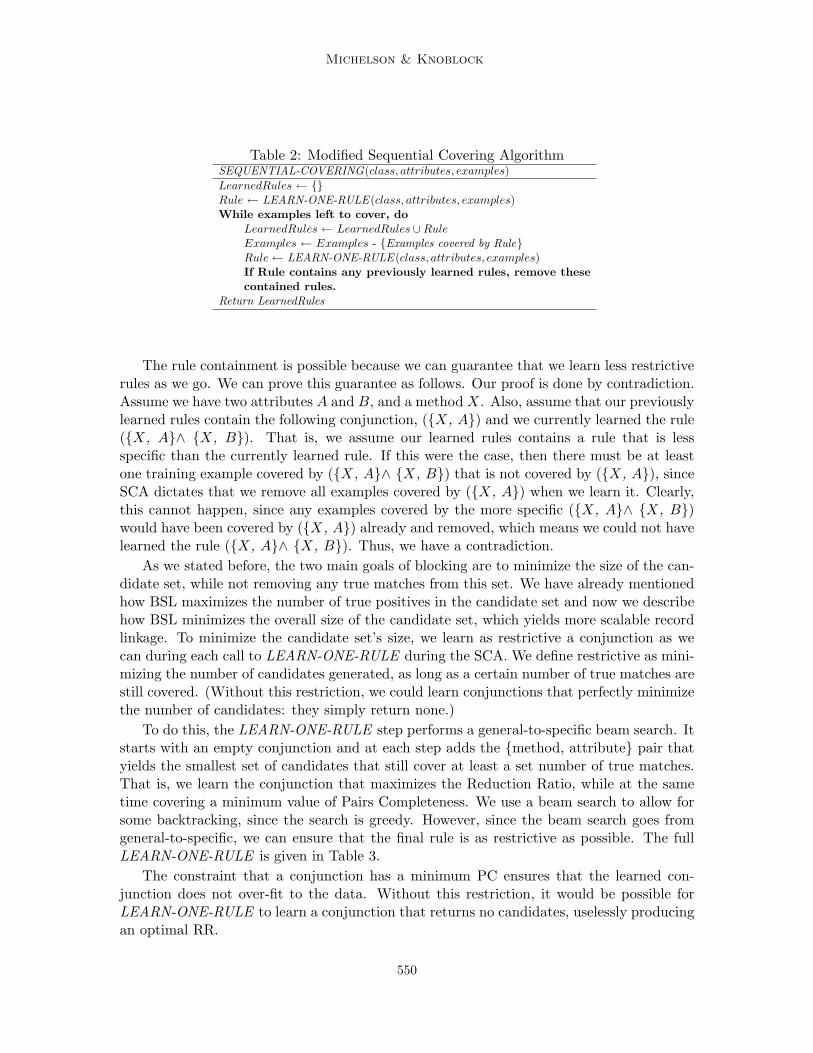
The BSL algorithm uses a modified version of the Sequential Covering Algorithm (SCA),used to discover disjunctive sets of rules from labeled training data (Mitchell, 1997). Inour case, SCA will learn disjunctive sets of conjunctions consisting of {method, attribute}pairs. Basically, each call to LEARN-ONE-RULE generates a conjunction, and BSL keepsiterating over this call, covering the true matches left over after each iteration. This waySCA learns a full blocking scheme. The BSL algorithm is shown in Table 2.
There are two modifications to the classic SCA algorithm, which are shown in bold.First, BSL runs until there are no more examples left to cover, rather than stopping atsome threshold. This ensures that we maximize the number of true matches generated ascandidates by the final blocking rule (Pairs Completeness). Note that this might, in turn,yield a large number of candidates, hurting the Reduction Ratio. However, omitting truematches directly affects the accuracy of record linkage, and blocking is a preprocessing stepfor record linkage, so it is more important to cover as many true matches as possible. Thisway BSL fulfills one of the blocking goals: not eliminating true matches if possible. Second,if we learn a new conjunction (in the LEARN-ONE-RULE step) and our current blockingscheme has a rule that already contains the newly learned rule, then we can remove therule containing the newly learned rule. This is an optimization that allows us to check rulecontainment as we go, rather than at the end.
549
Michelson & Knoblock
Table 2: Modified Sequential Covering AlgorithmSEQUENTIAL-COVERING(class, attributes, examples)LearnedRules ← {}Rule ← LEARN-ONE-RULE (class, attributes, examples)While examples left to cover, do
LearnedRules ← LearnedRules ∪ RuleExamples ← Examples - {Examples covered by Rule}Rule ← LEARN-ONE-RULE (class, attributes, examples)If Rule contains any previously learned rules, remove thesecontained rules.
Return LearnedRules
The rule containment is possible because we can guarantee that we learn less restrictiverules as we go. We can prove this guarantee as follows. Our proof is done by contradiction.Assume we have two attributes A and B, and a method X. Also, assume that our previouslylearned rules contain the following conjunction, ({X, A}) and we currently learned the rule({X, A}∧ {X, B}). That is, we assume our learned rules contains a rule that is lessspecific than the currently learned rule. If this were the case, then there must be at leastone training example covered by ({X, A}∧ {X, B}) that is not covered by ({X, A}), sinceSCA dictates that we remove all examples covered by ({X, A}) when we learn it. Clearly,this cannot happen, since any examples covered by the more specific ({X, A}∧ {X, B})would have been covered by ({X, A}) already and removed, which means we could not havelearned the rule ({X, A}∧ {X, B}). Thus, we have a contradiction.
As we stated before, the two main goals of blocking are to minimize the size of the can-didate set, while not removing any true matches from this set. We have already mentionedhow BSL maximizes the number of true positives in the candidate set and now we describehow BSL minimizes the overall size of the candidate set, which yields more scalable recordlinkage. To minimize the candidate set’s size, we learn as restrictive a conjunction as wecan during each call to LEARN-ONE-RULE during the SCA. We define restrictive as mini-mizing the number of candidates generated, as long as a certain number of true matches arestill covered. (Without this restriction, we could learn conjunctions that perfectly minimizethe number of candidates: they simply return none.)
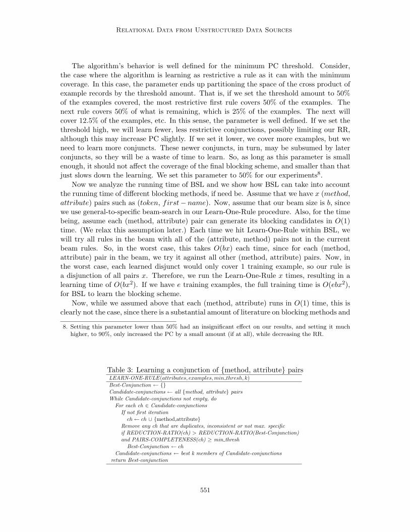
To do this, the LEARN-ONE-RULE step performs a general-to-specific beam search. Itstarts with an empty conjunction and at each step adds the {method, attribute} pair thatyields the smallest set of candidates that still cover at least a set number of true matches.That is, we learn the conjunction that maximizes the Reduction Ratio, while at the sametime covering a minimum value of Pairs Completeness. We use a beam search to allow forsome backtracking, since the search is greedy. However, since the beam search goes fromgeneral-to-specific, we can ensure that the final rule is as restrictive as possible. The fullLEARN-ONE-RULE is given in Table 3.
The constraint that a conjunction has a minimum PC ensures that the learned con-junction does not over-fit to the data. Without this restriction, it would be possible forLEARN-ONE-RULE to learn a conjunction that returns no candidates, uselessly producingan optimal RR.
550
Relational Data from Unstructured Data Sources
The algorithm’s behavior is well defined for the minimum PC threshold. Consider,the case where the algorithm is learning as restrictive a rule as it can with the minimumcoverage. In this case, the parameter ends up partitioning the space of the cross product ofexample records by the threshold amount. That is, if we set the threshold amount to 50%of the examples covered, the most restrictive first rule covers 50% of the examples. Thenext rule covers 50% of what is remaining, which is 25% of the examples. The next willcover 12.5% of the examples, etc. In this sense, the parameter is well defined. If we set thethreshold high, we will learn fewer, less restrictive conjunctions, possibly limiting our RR,although this may increase PC slightly. If we set it lower, we cover more examples, but weneed to learn more conjuncts. These newer conjuncts, in turn, may be subsumed by laterconjuncts, so they will be a waste of time to learn. So, as long as this parameter is smallenough, it should not affect the coverage of the final blocking scheme, and smaller than thatjust slows down the learning. We set this parameter to 50% for our experiments8.
Now we analyze the running time of BSL and we show how BSL can take into accountthe running time of different blocking methods, if need be. Assume that we have x (method,attribute) pairs such as (token, first− name). Now, assume that our beam size is b, sincewe use general-to-specific beam-search in our Learn-One-Rule procedure. Also, for the timebeing, assume each (method, attribute) pair can generate its blocking candidates in O(1)time. (We relax this assumption later.) Each time we hit Learn-One-Rule within BSL, wewill try all rules in the beam with all of the (attribute, method) pairs not in the currentbeam rules. So, in the worst case, this takes O(bx) each time, since for each (method,attribute) pair in the beam, we try it against all other (method, attribute) pairs. Now, inthe worst case, each learned disjunct would only cover 1 training example, so our rule isa disjunction of all pairs x. Therefore, we run the Learn-One-Rule x times, resulting in alearning time of O(bx2). If we have e training examples, the full training time is O(ebx2),for BSL to learn the blocking scheme.
Now, while we assumed above that each (method, attribute) runs in O(1) time, this isclearly not the case, since there is a substantial amount of literature on blocking methods and
8. Setting this parameter lower than 50% had an insignificant effect on our results, and setting it muchhigher, to 90%, only increased the PC by a small amount (if at all), while decreasing the RR.
Table 3: Learning a conjunction of {method, attribute} pairsLEARN-ONE-RULE (attributes, examples, min thresh, k)Best-Conjunction ← {}Candidate-conjunctions ← all {method, attribute} pairsWhile Candidate-conjunctions not empty, do
For each ch ∈ Candidate-conjunctionsIf not first iteration
ch ← ch ∪ {method,attribute}Remove any ch that are duplicates, inconsistent or not max. specificif REDUCTION-RATIO(ch) > REDUCTION-RATIO(Best-Conjunction)and PAIRS-COMPLETENESS(ch) ≥ min thresh
Best-Conjunction ← chCandidate-conjunctions ← best k members of Candidate-conjunctions
return Best-conjunction
551
Michelson & Knoblock
further the blocking times can vary significantly (Bilenko, Kamath, & Mooney, 2006). Letus define a function tx(e) that represents how long it takes for a single (method, attribute)pair in x to generate the e candidates in our training example. Using this notation, ourLearn-One-Rule time becomes O(b(xtx(e))) (we run tx(e) time for each pair in x) and so ourfull training time becomes O(eb(xtx(e))2). Clearly such a running time will be dominatedby the most expensive blocking methodology. Once a rule is learned, it is bounded by thetime it takes to run the rule and (method, attribute) pairs involved, so it takes O(xtx(n)),where n is the number of records we are classifying.
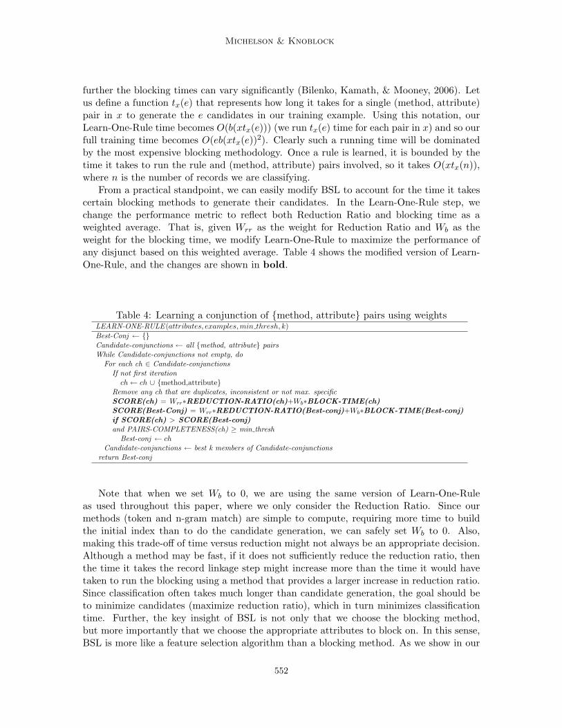
From a practical standpoint, we can easily modify BSL to account for the time it takescertain blocking methods to generate their candidates. In the Learn-One-Rule step, wechange the performance metric to reflect both Reduction Ratio and blocking time as aweighted average. That is, given Wrr as the weight for Reduction Ratio and Wb as theweight for the blocking time, we modify Learn-One-Rule to maximize the performance ofany disjunct based on this weighted average. Table 4 shows the modified version of Learn-One-Rule, and the changes are shown in bold.
Table 4: Learning a conjunction of {method, attribute} pairs using weightsLEARN-ONE-RULE (attributes, examples, min thresh, k)Best-Conj ← {}Candidate-conjunctions ← all {method, attribute} pairsWhile Candidate-conjunctions not empty, do
For each ch ∈ Candidate-conjunctionsIf not first iteration
ch ← ch ∪ {method,attribute}Remove any ch that are duplicates, inconsistent or not max. specificSCORE(ch) = Wrr∗REDUCTION-RATIO(ch)+Wb∗BLOCK-TIME(ch)SCORE(Best-Conj) = Wrr∗REDUCTION-RATIO(Best-conj)+Wb∗BLOCK-TIME(Best-conj)if SCORE(ch) > SCORE(Best-conj)and PAIRS-COMPLETENESS(ch) ≥ min thresh
Best-conj ← chCandidate-conjunctions ← best k members of Candidate-conjunctions
return Best-conj
Note that when we set Wb to 0, we are using the same version of Learn-One-Ruleas used throughout this paper, where we only consider the Reduction Ratio. Since ourmethods (token and n-gram match) are simple to compute, requiring more time to buildthe initial index than to do the candidate generation, we can safely set Wb to 0. Also,making this trade-off of time versus reduction might not always be an appropriate decision.Although a method may be fast, if it does not sufficiently reduce the reduction ratio, thenthe time it takes the record linkage step might increase more than the time it would havetaken to run the blocking using a method that provides a larger increase in reduction ratio.Since classification often takes much longer than candidate generation, the goal should beto minimize candidates (maximize reduction ratio), which in turn minimizes classificationtime. Further, the key insight of BSL is not only that we choose the blocking method,but more importantly that we choose the appropriate attributes to block on. In this sense,BSL is more like a feature selection algorithm than a blocking method. As we show in our
552

Relational Data from Unstructured Data Sources
experiments, for blocking it is more important to pick the right attribute combinations, asBSL does, even using simple methods, than to do blocking using the most sophisticatedmethods.
We can easily extend our BSL algorithm to handle the case of matching posts to membersof the reference set. This is a special case because the posts have all the attributes embeddedwithin them while the reference set data is relational and structured into schema elements.To handle this special case, rather than matching attribute and method pairs across thedata sources during our LEARN-ONE-RULE, we instead compare attribute and methodpairs from the relational data to the entire post. This is a small change, showing that thesame algorithm works well even in this special case.
Once we learn a good blocking scheme, we can now efficiently generate candidates fromthe post set to align to the reference set. This blocking step is essential for mapping largeamounts of unstructured and ungrammatical data sources to larger and larger referencesets.
2.2 The Matching Step
From the set of candidates generated during blocking one can find the member of thereference set that best matches the current post. That is, one data source’s record (thepost) must align to a record from the other data source (the reference set candidates).While the whole alignment procedure is referred to as record linkage (Fellegi & Sunter,1969), we refer to finding the particular matches after blocking as the “matching step.”
Figure 2: The traditional record linkage problem
However, the record linkage problem presented in this article differs from the “traditional”record linkage problem and is not well studied. Traditional record linkage matches a recordfrom one data source to a record from another data source by relating their respective,decomposed attributes. For instance, using the second post from Table 1, and assumingdecomposed attributes, the make from the post is compared to the make of the reference
553

Michelson & Knoblock
Figure 3: The problem of matching a post to the reference set
set. This is also done for the models, the trims, etc. The record from the reference set thatbest matches the post based on the similarities between the attributes would be consideredthe match. This is represented in Figure 2. Yet, the attributes of the posts are embeddedwithin a single piece of text and not yet identified. This text is compared to the referenceset, which is already decomposed into attributes and which does not have the extraneoustokens present in the post. Figure 3 depicts this problem. With this type of matchingtraditional record linkage approaches do not apply.
Instead, the matching step compares the post to all of the attributes of the reference setconcatenated together. Since the post is compared to a whole record from the reference set(in the sense that it has all of the attributes), this comparison is at the “record level” andit approximately reflects how similar all of the embedded attributes of the post are to all ofthe attributes of the candidate match. This mimics the idea of traditional record linkage,that comparing all of the fields determines the similarity at the record level.
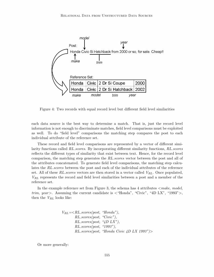
However, by using only the record level similarity it is possible for two candidates togenerate the same record level similarity while differing on individual attributes. If one ofthese attributes is more discriminative than the other, there needs to be some way to reflectthat. For example, consider Figure 4. In the figure, the two candidates share the same makeand model. However, the first candidate shares the year while the second candidate sharesthe trim. Since both candidates share the same make and model, and both have anotherattribute in common, it is possible that they generate the same record level comparison. Yet,a trim on car, especially with a rare thing like a “Hatchback” should be more discriminativethan sharing a year, since there are lots of cars with the same make, model and year, thatdiffer only by the trim. This difference in individual attributes needs to be reflected.
To discriminate between attributes, the matching step borrows the idea from traditionalrecord linkage that incorporating the individual comparisons between each attribute from
554
Relational Data from Unstructured Data Sources
Figure 4: Two records with equal record level but different field level similarities
each data source is the best way to determine a match. That is, just the record levelinformation is not enough to discriminate matches, field level comparisons must be exploitedas well. To do “field level” comparisons the matching step compares the post to eachindividual attribute of the reference set.
These record and field level comparisons are represented by a vector of different simi-larity functions called RL scores. By incorporating different similarity functions, RL scoresreflects the different types of similarity that exist between text. Hence, for the record levelcomparison, the matching step generates the RL scores vector between the post and all ofthe attributes concatenated. To generate field level comparisons, the matching step calcu-lates the RL scores between the post and each of the individual attributes of the referenceset. All of these RL scores vectors are then stored in a vector called VRL. Once populated,VRL represents the record and field level similarities between a post and a member of thereference set.
In the example reference set from Figure 3, the schema has 4 attributes <make, model,trim, year>. Assuming the current candidate is <“Honda”, “Civic”, “4D LX”, “1993”>,then the VRL looks like:
VRL=<RL scores(post, “Honda”),RL scores(post, “Civic”),RL scores(post, “4D LX”),RL scores(post, “1993”),RL scores(post, “Honda Civic 4D LX 1993”)>
Or more generally:
555
Michelson & Knoblock
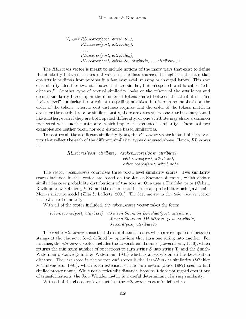
VRL=<RL scores(post, attribute1),RL scores(post, attribute2),. . . ,RL scores(post, attributen),RL scores(post, attribute1 attribute2 . . . attributen)>
The RL scores vector is meant to include notions of the many ways that exist to definethe similarity between the textual values of the data sources. It might be the case thatone attribute differs from another in a few misplaced, missing or changed letters. This sortof similarity identifies two attributes that are similar, but misspelled, and is called “editdistance.” Another type of textual similarity looks at the tokens of the attributes anddefines similarity based upon the number of tokens shared between the attributes. This“token level” similarity is not robust to spelling mistakes, but it puts no emphasis on theorder of the tokens, whereas edit distance requires that the order of the tokens match inorder for the attributes to be similar. Lastly, there are cases where one attribute may soundlike another, even if they are both spelled differently, or one attribute may share a commonroot word with another attribute, which implies a “stemmed” similarity. These last twoexamples are neither token nor edit distance based similarities.
To capture all these different similarity types, the RL scores vector is built of three vec-tors that reflect the each of the different similarity types discussed above. Hence, RL scoresis:
RL scores(post, attribute)=<token scores(post, attribute),edit scores(post, attribute),other scores(post, attribute)>
The vector token scores comprises three token level similarity scores. Two similarityscores included in this vector are based on the Jensen-Shannon distance, which definessimilarities over probability distributions of the tokens. One uses a Dirichlet prior (Cohen,Ravikumar, & Feinberg, 2003) and the other smooths its token probabilities using a Jelenik-Mercer mixture model (Zhai & Lafferty, 2001). The last metric in the token scores vectoris the Jaccard similarity.
With all of the scores included, the token scores vector takes the form:
token scores(post, attribute)=<Jensen-Shannon-Dirichlet(post, attribute),Jensen-Shannon-JM-Mixture(post, attribute),Jaccard(post, attribute)>
The vector edit scores consists of the edit distance scores which are comparisons betweenstrings at the character level defined by operations that turn one string into another. Forinstance, the edit scores vector includes the Levenshtein distance (Levenshtein, 1966), whichreturns the minimum number of operations to turn string S into string T, and the Smith-Waterman distance (Smith & Waterman, 1981) which is an extension to the Levenshteindistance. The last score in the vector edit scores is the Jaro-Winkler similarity (Winkler& Thibaudeau, 1991), which is an extension of the Jaro metric (Jaro, 1989) used to findsimilar proper nouns. While not a strict edit-distance, because it does not regard operationsof transformations, the Jaro-Winkler metric is a useful determinant of string similarity.
With all of the character level metrics, the edit scores vector is defined as:
556

Relational Data from Unstructured Data Sources
edit scores(post, attribute)=<Levenshtein(post, attribute),Smith-Waterman(post, attribute),Jaro-Winkler(post, attribute)>
All the similarities in the edit scores and token scores vector are defined in the Second-String package (Cohen et al., 2003) which was used for the experimental implementationas described in Section 4.
Lastly, the vector other scores captures the two types of similarity that did not fit intoeither the token level or edit distance similarity vector. This vector includes two typesof string similarities. The first is the Soundex score between the post and the attribute.Soundex uses the phonetics of a token as a basis for determining the similarity. Thatis, misspelled words that sound the same will receive a high Soundex score for similarity.The other similarity is based upon the Porter stemming algorithm (Porter, 1980), whichremoves the suffixes from strings so that the root words can be compared for similarity.This helps alleviate possible errors introduced by the prefix assumption introduced by theJaro-Winkler metric, since the stems are scored rather than the prefixes. Including both ofthese scores, the other scores vector becomes:
other scores(post, attribute)=<Porter-Stemmer(post, attribute),Soundex(post, attribute)>
Figure 5: The full vector of similarity scores used for record linkage
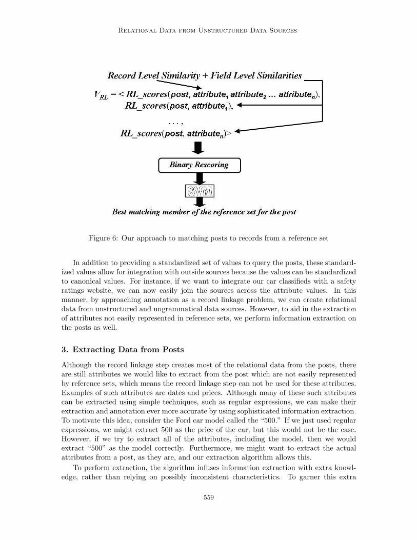
Figure 5 shows the full composition of VRL, with all the constituent similarity scores.Once a VRL is constructed for each of the candidates, the matching step then performs
a binary rescoring on each VRL to further help determine the best match amongst the can-didates. This rescoring helps determine the best possible match for the post by separating
557

Michelson & Knoblock
out the best candidate as much as possible. Because there might be a few candidates withsimilarly close values, and only one of them is a best match, the rescoring emphasizes thebest match by downgrading the close matches so that they have the same element val-ues as the more obvious non-matches, while boosting the difference in score with the bestcandidate’s elements.
To rescore the vectors of candidate set C, the rescoring method iterates through theelements xi of all VRL∈C, and the VRL(s) that contain the maximum value for xi map thisxi to 1, while all of the other VRL(s) map xi to 0. Mathematically, the rescoring method is:
∀VRLj ∈ C, j = 0... |C|∀xi ∈ VRLj , i = 0...
∣∣∣VRLj
∣∣∣f(xi, VRLj ) =
{1, xi = max(∀xt ∈ VRLs , VRLs ∈ C, t = i, s = 0... |C|)0, otherwise
For example, suppose C contains 2 candidates, VRL1 and VRL2 :
VRL1 = <{.999,...,1.2},...,{0.45,...,0.22}>VRL2 = <{.888,...,0.0},...,{0.65,...,0.22}>
After rescoring they become:
VRL1 = <{1,...,1},...,{0,...,1}>VRL2 = <{0,...,0},...,{1,...,1}>
After rescoring, the matching step passes each VRL to a Support Vector Machine (SVM)(Joachims, 1999) trained to label them as matches or non-matches. The best match is thecandidate that the SVM classifies as a match, with the maximally positive score for thedecision function. If more than one candidate share the same maximum score from thedecision function, then they are thrown out as matches. This enforces a strict 1-1 mappingbetween posts and members of the reference set. However, a 1-n relationship can be capturedby relaxing this restriction. To do this the algorithm keeps either the first candidate withthe maximal decision score, or chooses one randomly from the set of candidates with themaximum decision score.
Although we use SVMs in this paper to differentiate matches from non-matches, thealgorithm is not strictly tied to this method. The main characteristics for our learningproblem are that the feature vectors are sparse (because of the binary rescoring) and theconcepts are dense (since many useful features may be needed and thus none should bepruned by feature selection). We also tried to use a Naıve Bayes classifier for our matchingtask, but it was monumentally overwhelmed by the number of features and the numberof training examples. Yet this is not to say that other methods that can deal with sparsefeature vectors and dense concepts, such as online logistic regression or boosting, could notbe used in place of SVM.
After the match for a post is found, the attributes of the matching reference set memberare added as annotation to the post by including the values of the reference set attributeswith tags that reflect the schema of the reference set. The overall matching algorithm isshown in Figure 6.
558
Relational Data from Unstructured Data Sources
Figure 6: Our approach to matching posts to records from a reference set
In addition to providing a standardized set of values to query the posts, these standard-ized values allow for integration with outside sources because the values can be standardizedto canonical values. For instance, if we want to integrate our car classifieds with a safetyratings website, we can now easily join the sources across the attribute values. In thismanner, by approaching annotation as a record linkage problem, we can create relationaldata from unstructured and ungrammatical data sources. However, to aid in the extractionof attributes not easily represented in reference sets, we perform information extraction onthe posts as well.
3. Extracting Data from Posts
Although the record linkage step creates most of the relational data from the posts, thereare still attributes we would like to extract from the post which are not easily representedby reference sets, which means the record linkage step can not be used for these attributes.Examples of such attributes are dates and prices. Although many of these such attributescan be extracted using simple techniques, such as regular expressions, we can make theirextraction and annotation ever more accurate by using sophisticated information extraction.To motivate this idea, consider the Ford car model called the “500.” If we just used regularexpressions, we might extract 500 as the price of the car, but this would not be the case.However, if we try to extract all of the attributes, including the model, then we wouldextract “500” as the model correctly. Furthermore, we might want to extract the actualattributes from a post, as they are, and our extraction algorithm allows this.
To perform extraction, the algorithm infuses information extraction with extra knowl-edge, rather than relying on possibly inconsistent characteristics. To garner this extra
559

Michelson & Knoblock
knowledge, the approach exploits the idea of reference sets by using the attributes fromthe matching reference set member as a basis for identifying similar attributes in the post.Then, the algorithm can label these extracted values from the post with the schema fromthe reference set, thus adding annotation based on the extracted values.
In a broad sense, the algorithm has two parts. First we label each token with a possibleattribute label or as “junk” to be ignored. After all the tokens in a post are labeled, wethen clean each of the extracted labels. Figure 7 shows the whole procedure graphically,in detail, using the second post from Table 1. Each of the steps shown in this figure aredescribed in detail below.
Figure 7: Extraction process for attributes
To begin the extraction process, the post is broken into tokens. Using the first postfrom Table 1 as an example, set of tokens becomes, {“93”, “civic”, “5speed”,...}. Each ofthese tokens is then scored against each attribute of the record from the reference set thatwas deemed the match.
To score the tokens, the extraction process builds a vector of scores, VIE . Like the VRL
vector of the matching step, VIE is composed of vectors which represent the similaritiesbetween the token and the attributes of the reference set. However, the composition ofVIE is slightly different from VRL. It contains no comparison to the concatenation of allthe attributes, and the vectors that compose VIE are different from those that composeVRL. Specifically, the vectors that form VIE are called IE scores, and are similar to the
560

Relational Data from Unstructured Data Sources
RL scores that compose VRL, except they do not contain the token scores component, sinceeach IE scores only uses one token from the post at a time.
The RL scores vector:
RL scores(post, attribute)=<token scores(post, attribute),edit scores(post, attribute),other scores(post, attribute)>
becomes:
IE scores(token, attribute)=<edit scores(token, attribute),other scores(token, attribute)>
The other main difference between VIE and VRL is that VIE contains a unique vectorthat contains user defined functions, such as regular expressions, to capture attributes thatare not easily represented by reference sets, such as prices or dates. These attribute typesgenerally exhibit consistent characteristics that allow them to be extracted, and they areusually infeasible to represent in reference sets. This makes traditional extraction methodsa good choice for these attributes. This vector is called common scores because the typesof characteristics used to extract these attributes are “common” enough between to be usedfor extraction.
Using the first post of Table 1, assume the reference set match has the make “Honda,”the model “Civic” and the year “1993.” This means the matching tuple would be {“Honda”,“Civic”, “1993”}. This match generates the following VIE for the token “civic” of the post:
VIE=<common scores(“civic”),IE scores(“civic”,“Honda”),IE scores(“civic”,“Civic”),IE scores(“civic”,“1993”)>
More generally, for a given token, VIE looks like:
VIE=<common scores(token),IE scores(token, attribute1),IE scores(token, attribute2). . . ,IE scores(token, attributen)>
Each VIE is then passed to a structured SVM (Tsochantaridis, Joachims, Hofmann,& Altun, 2005; Tsochantaridis, Hofmann, Joachims, & Altun, 2004) trained to give it anattribute type label, such as make, model, or price. Intuitively, similar attribute typesshould have similar VIE vectors. The makes should generally have high scores against themake attribute of the reference set, and small scores against the other attributes. Further,structured SVMs are able to infer the extraction labels collectively, which helps in decidingbetween possible token labels. This makes the use of structured SVMs an ideal machinelearning method for our task. Note that since each VIE is not a member of a cluster wherethe winner takes all, there is no binary rescoring.
Since there are many irrelevant tokens in the post that should not be annotated, the SVMlearns that any VIE that does associate with a learned attribute type should be labeled as
561
Michelson & Knoblock
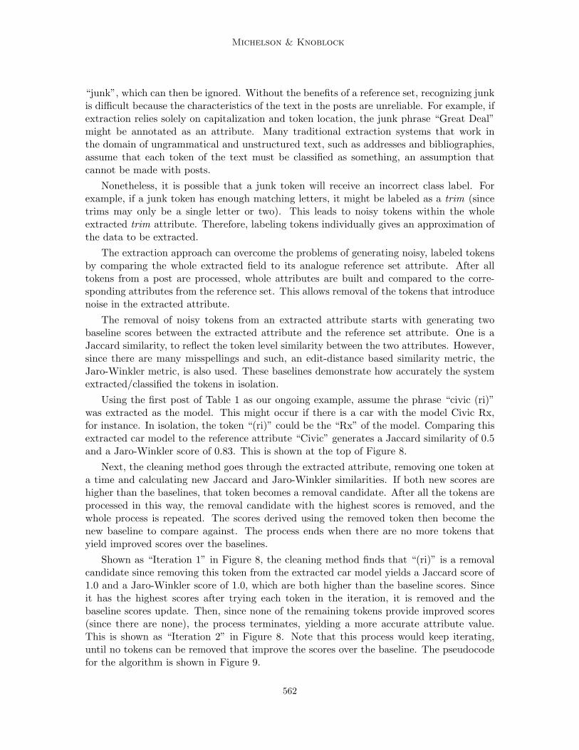
“junk”, which can then be ignored. Without the benefits of a reference set, recognizing junkis difficult because the characteristics of the text in the posts are unreliable. For example, ifextraction relies solely on capitalization and token location, the junk phrase “Great Deal”might be annotated as an attribute. Many traditional extraction systems that work inthe domain of ungrammatical and unstructured text, such as addresses and bibliographies,assume that each token of the text must be classified as something, an assumption thatcannot be made with posts.
Nonetheless, it is possible that a junk token will receive an incorrect class label. Forexample, if a junk token has enough matching letters, it might be labeled as a trim (sincetrims may only be a single letter or two). This leads to noisy tokens within the wholeextracted trim attribute. Therefore, labeling tokens individually gives an approximation ofthe data to be extracted.
The extraction approach can overcome the problems of generating noisy, labeled tokensby comparing the whole extracted field to its analogue reference set attribute. After alltokens from a post are processed, whole attributes are built and compared to the corre-sponding attributes from the reference set. This allows removal of the tokens that introducenoise in the extracted attribute.
The removal of noisy tokens from an extracted attribute starts with generating twobaseline scores between the extracted attribute and the reference set attribute. One is aJaccard similarity, to reflect the token level similarity between the two attributes. However,since there are many misspellings and such, an edit-distance based similarity metric, theJaro-Winkler metric, is also used. These baselines demonstrate how accurately the systemextracted/classified the tokens in isolation.
Using the first post of Table 1 as our ongoing example, assume the phrase “civic (ri)”was extracted as the model. This might occur if there is a car with the model Civic Rx,for instance. In isolation, the token “(ri)” could be the “Rx” of the model. Comparing thisextracted car model to the reference attribute “Civic” generates a Jaccard similarity of 0.5and a Jaro-Winkler score of 0.83. This is shown at the top of Figure 8.
Next, the cleaning method goes through the extracted attribute, removing one token ata time and calculating new Jaccard and Jaro-Winkler similarities. If both new scores arehigher than the baselines, that token becomes a removal candidate. After all the tokens areprocessed in this way, the removal candidate with the highest scores is removed, and thewhole process is repeated. The scores derived using the removed token then become thenew baseline to compare against. The process ends when there are no more tokens thatyield improved scores over the baselines.
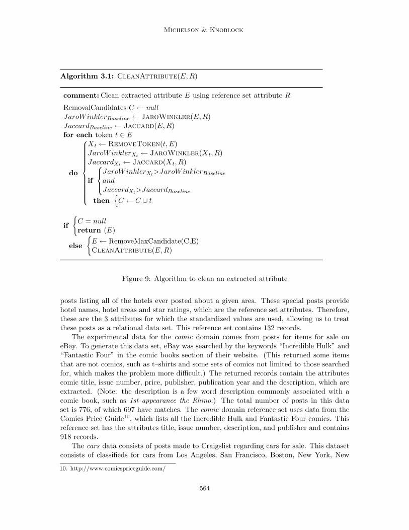
Shown as “Iteration 1” in Figure 8, the cleaning method finds that “(ri)” is a removalcandidate since removing this token from the extracted car model yields a Jaccard score of1.0 and a Jaro-Winkler score of 1.0, which are both higher than the baseline scores. Sinceit has the highest scores after trying each token in the iteration, it is removed and thebaseline scores update. Then, since none of the remaining tokens provide improved scores(since there are none), the process terminates, yielding a more accurate attribute value.This is shown as “Iteration 2” in Figure 8. Note that this process would keep iterating,until no tokens can be removed that improve the scores over the baseline. The pseudocodefor the algorithm is shown in Figure 9.
562

Relational Data from Unstructured Data Sources
Figure 8: Improving extraction accuracy with reference set attributes
Note, however, that we do not limit the machine learning component of our extractionalgorithm to SVMs. Instead, we claim that in some cases, reference sets can aid extractionin general, and to test this, in our architecture we can replace the SVM component withother methods. For example, in our extraction experiments we replace the SVM extractorwith a Conditional Random Field (CRF) (Lafferty, McCallum, & Pereira, 2001) extractorthat uses the VIE as features.
Therefore, the whole extraction process takes a token of the text, creates the VIE andpasses this to the machine-learning extractor which generates a label for the token. Theneach field is cleaned and the extracted attribute is saved.
4. Results
The Phoebus system was built to experimentally validate our approach to building relationaldata from unstructured and ungrammatical data sources. Specifically, Phoebus tests thetechnique’s accuracy in both the record linkage and the extraction, and incorporates theBSL algorithm for learning and using blocking schemes. The experimental data, comes fromthree domains of posts: hotels, comic books, and cars.
The data from the hotel domain contains the attributes hotel name, hotel area, starrating, price and dates, which are extracted to test the extraction algorithm. This datacomes from the Bidding For Travel website9 which is a forum where users share successfulbids for Priceline on items such as airline tickets and hotel rates. The experimental datais limited to postings about hotel rates in Sacramento, San Diego and Pittsburgh, whichcompose a data set with 1125 posts, with 1028 of these posts having a match in the referenceset. The reference set comes from the Bidding For Travel hotel guides, which are special
9. www.biddingfortravel.com
563
Michelson & Knoblock
Algorithm 3.1: CleanAttribute(E,R)
comment: Clean extracted attribute E using reference set attribute R
RemovalCandidates C ← nullJaroWinklerBaseline ← JaroWinkler(E,R)JaccardBaseline ← Jaccard(E,R)for each token t ∈ E
do
⎧⎪⎪⎪⎪⎪⎪⎪⎪⎪⎪⎨⎪⎪⎪⎪⎪⎪⎪⎪⎪⎪⎩
Xt ← RemoveToken(t, E)JaroWinklerXt ← JaroWinkler(Xt, R)JaccardXt ← Jaccard(Xt, R)
if
⎧⎪⎨⎪⎩
JaroWinklerXt>JaroWinklerBaseline
andJaccardXt>JaccardBaseline
then{C ← C ∪ t
if
{C = nullreturn (E)
else
{E ← RemoveMaxCandidate(C,E)CleanAttribute(E,R)
Figure 9: Algorithm to clean an extracted attribute
posts listing all of the hotels ever posted about a given area. These special posts providehotel names, hotel areas and star ratings, which are the reference set attributes. Therefore,these are the 3 attributes for which the standardized values are used, allowing us to treatthese posts as a relational data set. This reference set contains 132 records.
The experimental data for the comic domain comes from posts for items for sale oneBay. To generate this data set, eBay was searched by the keywords “Incredible Hulk” and“Fantastic Four” in the comic books section of their website. (This returned some itemsthat are not comics, such as t–shirts and some sets of comics not limited to those searchedfor, which makes the problem more difficult.) The returned records contain the attributescomic title, issue number, price, publisher, publication year and the description, which areextracted. (Note: the description is a few word description commonly associated with acomic book, such as 1st appearance the Rhino.) The total number of posts in this dataset is 776, of which 697 have matches. The comic domain reference set uses data from theComics Price Guide10, which lists all the Incredible Hulk and Fantastic Four comics. Thisreference set has the attributes title, issue number, description, and publisher and contains918 records.
The cars data consists of posts made to Craigslist regarding cars for sale. This datasetconsists of classifieds for cars from Los Angeles, San Francisco, Boston, New York, New
10. http://www.comicspriceguide.com/
564

Relational Data from Unstructured Data Sources
Jersey and Chicago. There are a total of 2,568 posts in this data set, and each postcontains a make, model, year, trim and price. The reference set for the Cars domain comesfrom the Edmunds11 car buying guide. From this data set we extracted the make, model,year and trim for all cars from 1990 to 2005, resulting in 20,076 records. There are 15,338matches between the posts to Craigslist and the cars from Edmunds.
Unlike the hotels and comics domains, a strict 1-1 relationship between the post andreference set was not enforced in the cars domain. As described previously, Phoebus re-laxed the 1-1 relationship to form a 1-n relationship between the posts and the referenceset. Sometimes the records do not contain enough attributes to discriminate a single bestreference member. For instance, posts that contain just a model and a year might match acouple of reference set records that would differ on the trim attribute, but have the samemake, model, and year. Yet, we can still use this make, model and year accurately forextraction. So, in this case, as mentioned previously, we pick one of the matches. This way,we exploit the attributes that we can from the reference set, since we have confidence inthose.
For the experiments, posts in each domain are split into two folds, one for training andone for testing. This is usually called two-fold cross validation. However, in many cases two-fold cross validation results in using 50% of the data for training and 50% for testing. Webelieve that this is too much data to have to label, especially as data sets become large, soour experiments instead focus on using less training data. One set of experiments uses 30%of the posts for training and tests on the remaining 70%, and the second set of experimentsuses just 10% of the posts to train, testing on the remaining 90%. We believe that trainingon small amounts of data, such as 10%, is an important empirical procedure since realworld data sets are large and labeling 50% of such large data sets is time consuming andunrealistic. In fact, the size of the Cars domain prevented us from using 30% of the data fortraining, since the machine learning algorithms could not scale to the number of trainingtuples this would generate. So for the Cars domain we only run experiments training on10% of the data. All experiments are performed 10 times, and the average results for these10 trials are reported.
4.1 Record Linkage Results
In this subsection we report our record linkage results, broken down into separate discussionsof our blocking results and our matching results.
4.1.1 Blocking Results
In order for the BSL algorithm to learn a blocking scheme, it must be provided with methodsit can use to compare the attributes. For all domains and experiments we use two commonmethods. The first, which we call “token,” compares any matching token between theattributes. The second method, “ngram3,” considers any matching 3-grams between theattributes.
It is important to note that a comparison between BSL and other blocking methods, suchas the Canopies method (McCallum, Nigam, & Ungar, 2000) and Bigram indexing (Baxter,Christen, & Churches, 2003), is slightly misaligned because the algorithms solve different
11. www.edmunds.com
565
Michelson & Knoblock
problems. Methods such as Bigram indexing are techniques that make the process of eachblocking pass on an attribute more efficient. The goal of BSL, however, is to select whichattribute combinations should be used for blocking as a whole, trying different attribute andmethod pairs. Nonetheless, we contend that it is more important to select the right attributecombinations, even using simple methods, than it is to use more sophisticated methods, butwithout insight as to which attributes might be useful. To test this hypothesis, we compareBSL using the token and 3-gram methods to Bigram indexing over all of the attributes.This is equivalent to forming a disjunction over all attributes using Bigram indexing as themethod. We chose Bigram indexing in particular because it is designed to perform “fuzzyblocking” which seems necessary in the case of noisy post data. As stated previously (Baxteret al., 2003), we use a threshold of 0.3 for Bigram indexing, since that works the best. Wealso compare BSL to running a disjunction over all attributes using the simple token methodonly. In our results, we call this blocking rule “Disjunction.” This disjunction mirrors theidea of picking the simplest possible blocking method: namely using all attributes with avery simple method.
As stated previously, the two goals of blocking can be quantified by the Reduction Ratio(RR) and the Pairs Completeness (PC). Table 5 shows not only these values but also howmany candidates were generated on average over the entire test set, comparing the threedifferent approaches. Table 5 also shows how long it took each method to learn the ruleand run the rule. Lastly, the column “Time match” shows how long the classifier needs torun given the number of candidates generated by the blocking scheme.
Table 6 shows a few example blocking schemes that the algorithm generated. For acomparison of the attributes BSL selected to the attributes picked manually for differentdomains where the data is structured the reader is pointed to our previous work on thetopic (Michelson & Knoblock, 2006).
The results of Table 5 validate our idea that it is more important to pick the correctattributes to block on (using simple methods) than to use sophisticated methods withoutattention to the attributes. Comparing the BSL rule to the Bigram results, the combinationof PC and RR is always better using BSL. Note that although in the Cars domain Bigramtook significantly less time with the classifier due to its large RR, it did so because it onlyhad a PC of 4%. In this case, Bigrams was not even covering 5% of the true matches.
Further, the BSL results are better than using the simplest method possible (the Disjuc-tion), especially in the cases where there are many records to test upon. As the number ofrecords scales up, it becomes increasingly important to gain a good RR, while maintaininga good PC value as well. This savings is dramatically demonstrated by the Cars domain,where BSL outperformed the Disjunction in both PC and RR.
One surprising aspect of these results is how prevalent the token method is within all thedomains. We expect that the ngram method would be used almost exclusively since thereare many spelling mistakes within the posts. However, this is not the case. We hypothesizethat the learning algorithm uses the token methods because they occur with more regularityacross the posts than the common ngrams would since the spelling mistakes might vary quitedifferently across the posts. This suggests that there might be more regularity, in terms ofwhat we can learn from the data, across the posts than we initially surmised.
Another interesting result is the poor reduction ratio of the Comic domain. This happensbecause most of the rules contain the disjunct that finds a common token within the comic
566

Relational Data from Unstructured Data Sources
RR PC # Cands Time Learn (s) Time Run (s) Time match (s)Hotels (30%)
BSL 81.56 99.79 19,153 69.25 24.05 60.93Disjunction 67.02 99.82 34,262 0 12.49 109.00
Bigrams 61.35 72.77 40,151 0 1.2 127.74Hotels (10%)
BSL 84.47 99.07 20,742 37.67 31.87 65.99Disjunction 66.91 99.82 44,202 0 15.676 140.62
Bigrams 60.71 90.39 52,492 0 1.57 167.00Comics (30%)
BSL 42.97 99.75 284,283 85.59 36.66 834.94Disjunction 37.39 100.00 312,078 0 45.77 916.57
Bigrams 36.72 69.20 315,453 0 102.23 926.48Comics (10%)
BSL 42.97 99.74 365,454 34.26 35.65 1,073.34Disjunction 37.33 100.00 401,541 0 52.183 1,179.32
Bigrams 36.75 88.41 405,283 0 131.34 1,190.31Cars (10%)
BSL 88.48 92.23 5,343,424 465.85 805.36 25,114.09Disjunction 87.92 89.90 5,603,146 0 343.22 26.334.79
Bigrams 97.11 4.31 1,805,275 0 996.45 8,484.79
Table 5: Blocking results using the BSL algorithm (amount of data used for training shownin parentheses).
Hotels Domain (30%)({hotel area,token} ∧ {hotel name,token} ∧ {star rating, token}) ∪ ({hotel name, ngram3})
Hotels Domain (10%)({hotel area,token} ∧ {hotel name,token}) ∪ ({hotel name,ngram3})
Comic Domain (30%)({title, token})
Comic Domain (10%)({title, token}) ∪ ({issue number,token} ∧ {publisher,token} ∧ {title,ngram3})
Cars Domain (10%)({make,token}) ∪ ({model,ngram3}) ∪ ({year,token} ∧ {make,ngram3})
Table 6: Some example blocking schemes learned for each of the domains.
567

Michelson & Knoblock
title. This rule produces such a poor reduction ratio because the value for this attribute isthe same across almost all reference set records. That is to say, when there are just a fewunique values for the BSL algorithm to use for blocking, the reduction ratio will be small.In this domain, there are only two values for the comic title attribute, “Fantastic Four” and“Incredible Hulk.” So it makes sense that if blocking is done using the title attribute only,the reduction is about half, since blocking on the value “Fantastic Four” just gets rid of the“Incredible Hulk” comics. This points to an interesting limitation of the BSL algorithm. Ifthere are not many distinct values for the different attribute and method pairs that BSLcan use to learn from, then this lack of values cripples the performance of the reductionratio. Intuitively though, this makes sense, since it is hard to distinguish good candidatematches from bad candidate matches if they share the same attribute values.
Another result worth mentioning is that in the Hotels domain we get a lower RR butthe same PC when we use less training data. This happens because our BSL algorithmruns until it has no more examples to cover, so if those last few examples introduce a newdisjunct that produces a lot of candidates, while only covering a few more true positives,then this would cause the RR to decrease, while keeping the PC at the same high rate.This is in fact what happens in this case. One way to curb this behavior would be to setsome sort of stopping threshold for BSL, but as we said, maximizing the PC is the mostimportant thing, so we choose not to do this. We want BSL to cover as many true positivesas it can, even if that means losing a bit in the reduction.
In fact, we next test this notion explicitly. We set a threshold in the SCA such thatafter 95% of the training examples are covered, the algorithm stops and returns the learnedblocking scheme. This helps to avoid the situation where BSL learns a very general conjunc-tion, solely to cover the last few remaining training examples. When that happens, BSLmight end up lowering the RR, at the expense of covering just those last training examples,because the rule learned to cover those last examples is overly general and returns too manycandidate matches.
Domain Record Linkage RR PCF-Measure
Hotels DomainNo Thresh (30%) 90.63 81.56 99.7995% Thresh (30%) 90.63 87.63 97.66
Comic DomainNo Thresh (30%) 91.30 42.97 99.7595% Thresh (30%) 91.47 42.97 99.69
Cars DomainNo Thresh (10%) 77.04 88.48 92.2395% Thresh (10%) 67.14 92.67 83.95
Table 7: A comparison of BSL covering all training examples, and covering 95% of thetraining examples
568

Relational Data from Unstructured Data Sources
Table 7 shows that when we use a threshold in the Hotels and Cars domain we see astatistically significant drop in Pairs Completeness with a statistically significant increasein Reduction Ratio.12 This is expected behavior since the threshold causes BSL to kickout of SCA before it can cover the last few training examples, which in turn allows BSLto retain a rule with high RR, but lower PC. However, when we look at the record linkageresults, we see that this threshold does in fact have a large effect.13 Although there is nostatistically significant difference in the F-measure for record linkage in the Hotels domain,the difference in Cars domain is dramatic. When we use a threshold, the candidates notdiscovered by the rule generated when using the threshold have an effect of 10% on the finalF-measure match results.14 Therefore, since the F-measure results differ by so much, weconclude that it is worthwhile to maximize PC when learning rules with BSL, even if theRR may decrease. That is to say, even in the presence of noise, which in turn may lead tooverly generic blocking schemes, BSL should try to maximize the true matches it covers,because avoiding even the most difficult cases to cover may affect the matching results. Aswe see in Table 7, this is especially true in the Cars domain where matching is much moredifficult than in the Hotels domain.
Interestingly, in the Comic domain we do not see a statistically significant differencein the RR and PC. This is because across trials we almost always learn the same rulewhether we use a threshold or not, and this rule covers enough training examples that thethreshold is not hit. Further, there is no statistically significant change in the F-measurerecord linkage results for this domain. This is expected since BSL would generate the samecandidate matches, whether it uses the threshold or not, since in both cases it almost alwayslearns the same blocking rules.
Our results using BSL are encouraging because they show that the algorithm also worksfor blocking when matching unstructured and ungrammatical text to a relational datasource. This means the algorithm works in this special case too, not just the case oftraditional record linkage where we are matching one structured source to another. Thismeans our overall algorithm for semantic annotation is much more scalable because we areusing fewer candidate matches than in our previous work (Michelson & Knoblock, 2005).
4.1.2 Matching Results
Since this alignment approach hinges on leveraging reference sets, it becomes necessary toshow the matching step performs well. To measure this accuracy, the experiments employthe usual record linkage statistics:
Precision =#CorrectMatches
#TotalMatchesMade
Recall =#CorrectMatches
#PossibleMatches
12. Bold means statistically significant using a two-tailed t-test with α set to 0.0513. Please see subsection 4.1.2 for a description of the record linkage experiments and results.14. Much of this difference is attributed to the non-threshold version of the algorithm learning a final
predicate that includes the make attribute by itself, which the version with a threshold does not learn.Since each make attribute value covers many records, it generates many candidates which results inincreasing PC while reducing RR.
569

Michelson & Knoblock
F − Measure =2 ∗ Precision ∗ Recall
Precison + Recall
The record linkage approach in this article is compared to WHIRL (Cohen, 2000).WHIRL performs record linkage by performing soft-joins using vector-based cosine similari-ties between the attributes. Other record linkage systems require decomposed attributes formatching, which is not the case with the posts. WHIRL serves as the benchmark because itdoes not have this requirement. To mirror the alignment task of Phoebus, the experimentsupplies WHIRL with two tables: the test set of posts (either 70% or 90% of the posts) andthe reference set with the attributes concatenated to approximate a record level match. Theconcatenation is also used because when matching on each individual attribute, it is notobvious how to combine the matching attributes to construct a whole matching referenceset member.
To perform the record linkage, WHIRL does soft-joins across the tables, which producesa list of matches, ordered by descending similarity score. For each post with matches fromthe join, the reference set member(s) with the highest similarity score(s) is called its match.In the Cars domain the matches are 1-N, so this means that only 1 match from the referenceset will be exploited later in the information extraction step. To mirror this idea, the numberof possible matches in a 1-N domain is counted as the number of posts that have a match inthe reference set, rather than the reference set members themselves that match. Also, thismeans that we only add a single match to our total number of correct matches for a givenpost, rather than all of the correct matches, since only one matters. This is done for bothWHIRL and Phoebus, and more accurately reflects how well each algorithm would performas the processing step before our information extraction step.
The record linkage results for both Phoebus and WHIRL are shown in Table 8. Notethat the amount of training data for each domain is shown in parentheses. All resultsare statistically significant using a two-tailed paired t-test with α=0.05, except for theprecision between WHIRL and Phoebus in the Cars domain, and the precision betweenPhoebus trained on 10% and 30% of the training data in the Comic domain.
Phoebus outperforms WHIRL because it uses many similarity types to distinguishmatches. Also, since Phoebus uses both a record level and attribute level similarities,it is able to distinguish between records that differ in more discriminative attributes. Thisis especially apparent in the Cars domain. First, these results indicate the difficulty ofmatching car posts to the large reference set. This is the largest experimental domain yetused for this problem, and it is encouraging how well our approach outperforms the base-line. It is also interesting that the results suggest that both techniques are equally accuratein terms of precision (in fact, there is no statistically significant difference between themin this sense) but Phoebus is able to retrieve many more relevant matches. This meansPhoebus can capture more rich features that predict matches than WHIRL’s cosine simi-larity alone. We expect this behavior because Phoebus has a notion of both field and tokenlevel similarity, using many different similarity measures. This justifies our use of the manysimilarity types and field and record level information, since our goal is to find as manymatches as we can.
It is also encouraging that using only 10% of the data for labeling, Phoebus is able toperform almost as well as using 30% of the data for training. Since the amount of data onthe Web is vast, only having to label 10% of the data to get comparative results is preferable
570

Relational Data from Unstructured Data Sources
Precision Recall F-measureHotel
Phoebus (30%) 87.70 93.78 90.63Phoebus (10%) 87.85 92.46 90.09
WHIRL 83.53 83.61 83.13Comic
Phoebus (30%) 87.49 95.46 91.30Phoebus (10%) 85.35 93.18 89.09
WHIRL 73.89 81.63 77.57Cars
Phoebus (10%) 69.98 85.68 77.04WHIRL 70.43 63.36 66.71
Table 8: Record linkage results
when the cost of labeling data is great. Especially since the clean annotation, and hencerelational data, comes from correctly matching the posts to the reference set, not havingto label much of the data is important if we want this technique to be widely applicable.In fact, we faced this practical issue ourselves in the Cars domain where we were unableto use 30% for training since the machine learning method would not scale to the numberof candidates generated by this much training data. So, the fact that we can report goodresults with just 10% training data allows us to extend this work to the much larger Carsdomain.
While our method performs well and outperforms WHIRL, from the results above, it isnot clear whether it is the use of the many string metrics, the inclusion of the attributes andtheir concatenation or the SVM itself that provides this advantage. To test the advantagesof each piece, we ran several experiments isolating each of these ideas.
First, we ran Phoebus matching on only the concatenation of the attributes from thereference set, rather than the concatenation and all the attributes individually. Earlier, westated that we use the concatenation to mirror the idea of record level similarity and we alsouse each attribute to mirror field level similarity. It is our hypothesis that in some cases,a post will match different reference set records with the same record level score (usingthe concatenation), but it will do so matching on different attributes. By removing theindividual attributes and leaving only the concatenation of them for matching, we can testhow the concatenation influences the matching in isolation. Table 9 shows these results forthe different domains.
For the Cars and Comic domains we see an improvement in F-measure, indicating thatthat using the attributes and the concatenation is much better for matching than using theconcatenation alone. This supports our notion that we also need a method to capture thesignificance of matching individual attributes since some attributes are better indicators ofmatching than others. It is also interesting to note that for both these domains, WHIRL doesa better job than the machine learning using only the concatenation, even though WHIRL
571
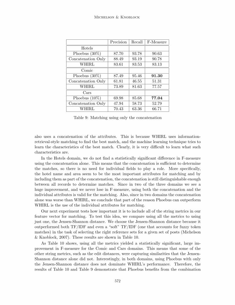
Michelson & Knoblock
Precision Recall F-MeasureHotels
Phoebus (30%) 87.70 93.78 90.63Concatenation Only 88.49 93.19 90.78
WHIRL 83.61 83.53 83.13Comic
Phoebus (30%) 87.49 95.46 91.30Concatenation Only 61.81 46.55 51.31
WHIRL 73.89 81.63 77.57Cars
Phoebus (10%) 69.98 85.68 77.04Concatenation Only 47.94 58.73 52.79
WHIRL 70.43 63.36 66.71
Table 9: Matching using only the concatenation
also uses a concatenation of the attributes. This is because WHIRL uses information-retrieval-style matching to find the best match, and the machine learning technique tries tolearn the characteristics of the best match. Clearly, it is very difficult to learn what suchcharacteristics are.
In the Hotels domain, we do not find a statistically significant difference in F-measureusing the concatenation alone. This means that the concatenation is sufficient to determinethe matches, so there is no need for individual fields to play a role. More specifically,the hotel name and area seem to be the most important attributes for matching and byincluding them as part of the concatenation, the concatenation is still distinguishable enoughbetween all records to determine matches. Since in two of the three domains we see ahuge improvement, and we never lose in F-measure, using both the concatenation and theindividual attributes is valid for the matching. Also, since in two domains the concatenationalone was worse than WHIRL, we conclude that part of the reason Phoebus can outperformWHIRL is the use of the individual attributes for matching.
Our next experiment tests how important it is to include all of the string metrics in ourfeature vector for matching. To test this idea, we compare using all the metrics to usingjust one, the Jensen-Shannon distance. We choose the Jensen-Shannon distance because itoutperformed both TF/IDF and even a “soft” TF/IDF (one that accounts for fuzzy tokenmatches) in the task of selecting the right reference sets for a given set of posts (Michelson& Knoblock, 2007). These results are shown in Table 10.
As Table 10 shows, using all the metrics yielded a statistically significant, large im-provement in F-measure for the Comic and Cars domains. This means that some of theother string metrics, such as the edit distances, were capturing similarities that the Jensen-Shannon distance alone did not. Interestingly, in both domains, using Phoebus with onlythe Jensen-Shannon distance does not dominate WHIRL’s performance. Therefore, theresults of Table 10 and Table 9 demonstrate that Phoebus benefits from the combination
572

Relational Data from Unstructured Data Sources
Precision Recall F-MeasureHotels
Phoebus (30%) 87.70 93.78 90.63Jensen-Shannon Only 89.65 92.28 90.94
WHIRL 83.61 83.53 83.13Comic
Phoebus (30%) 87.49 95.46 91.30Jensen-Shannon Only 65.36 69.96 67.58
WHIRL 73.89 81.63 77.57Cars
Phoebus (10%) 69.98 85.68 77.04Jensen-Shannon Only 72.87 59.43 67.94
WHIRL 70.43 63.36 66.71
Table 10: Using all string metrics versus using only the Jensen-Shannon distance
of many, varied similarity metrics along with the use of individual attributes for field levelsimilarities, and both of these aspects contribute to Phoebus outperforming WHIRL.
In the case of the Hotels data, there is not a statistically significant difference in thematching results, so in this case the other metrics do not provide relevant information formatching. Therefore, all the matches missed by the Jensen-Shannon only method are alsomissed when we include all of the metrics. Hence, either these missed matches are verydifficult to discover, or we do not have a string metric in our method yet that can capturethe similarity. For example, when the post has a token “DT” and the reference set record itshould match has a hotel area of “Downtown,” then an abbreviation metric could capturethis relationship. However, Phoebus does not include an abbreviation similarity measure.
Since none of the techniques in isolation consistently outperforms WHIRL, we concludethat Phoebus outperforms WHIRL because it combines multiple string metrics, it uses bothindividual attributes and the concatenation, and, as stated in Section 2.2, the SVM classifieris well suited for our record linkage task. These results also justify our inclusion of manymetrics and the individual attributes, along with our use of SVM as our classifier.
Our last matching experiment justifies our binary rescoring mechanism. Table 11 showsthe results of performing the binary rescoring for record linkage versus not performing thisbinary recoring. We hypothesize earlier in this paper that the binary rescoring will allowthe classifier to more accurately make match decisions because the rescoring separates outthe best candidate as much as possible. Table 11 shows this to be the case, as across alldomains when we perform the binary rescoring we gain a statistically significant amountin the F-measure. This shows that the record linkage is more easily able to identify thetrue matches from the possible candidates when the only difference in the record linkagealgorithm is the use of binary rescoring.
573
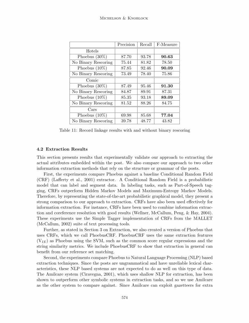
Michelson & Knoblock
Precision Recall F-MeasureHotels
Phoebus (30%) 87.70 93.78 90.63No Binary Rescoring 75.44 81.82 78.50
Phoebus (10%) 87.85 92.46 90.09No Binary Rescoring 73.49 78.40 75.86
ComicPhoebus (30%) 87.49 95.46 91.30
No Binary Rescoring 84.87 89.91 87.31Phoebus (10%) 85.35 93.18 89.09
No Binary Rescoring 81.52 88.26 84.75Cars
Phoebus (10%) 69.98 85.68 77.04No Binary Rescoring 39.78 48.77 43.82
Table 11: Record linkage results with and without binary rescoring
4.2 Extraction Results
This section presents results that experimentally validate our approach to extracting theactual attributes embedded within the post. We also compare our approach to two otherinformation extraction methods that rely on the structure or grammar of the posts.
First, the experiments compare Phoebus against a baseline Conditional Random Field(CRF) (Lafferty et al., 2001) extractor. A Conditional Random Field is a probabilisticmodel that can label and segment data. In labeling tasks, such as Part-of-Speech tag-ging, CRFs outperform Hidden Markov Models and Maximum-Entropy Markov Models.Therefore, by representing the state-of-the-art probabilistic graphical model, they present astrong comparison to our approach to extraction. CRFs have also been used effectively forinformation extraction. For instance, CRFs have been used to combine information extrac-tion and coreference resolution with good results (Wellner, McCallum, Peng, & Hay, 2004).These experiments use the Simple Tagger implementation of CRFs from the MALLET(McCallum, 2002) suite of text processing tools.
Further, as stated in Section 3 on Extraction, we also created a version of Phoebus thatuses CRFs, which we call PhoebusCRF. PhoebusCRF uses the same extraction features(VIE) as Phoebus using the SVM, such as the common score regular expressions and thestring similarity metrics. We include PhoebusCRF to show that extraction in general canbenefit from our reference set matching.
Second, the experiments compare Phoebus to Natural Language Processing (NLP) basedextraction techniques. Since the posts are ungrammatical and have unreliable lexical char-acteristics, these NLP based systems are not expected to do as well on this type of data.The Amilcare system (Ciravegna, 2001), which uses shallow NLP for extraction, has beenshown to outperform other symbolic systems in extraction tasks, and so we use Amilcareas the other system to compare against. Since Amilcare can exploit gazetteers for extra
574
Relational Data from Unstructured Data Sources
information, for our experiments Amilcare receives the reference data as a gazetteer to aidthe extraction. Both Simple Tagger and Amilcare are used with default settings.
Lastly, we compare Phoebus trained using 30% of the data for training to Phoebustrained using 10% of the data. (We do this for PhoebusCRF as well.) In our experimentalresults, the amount of training data is put in parentheses.
One component of the extraction vector VIE is the vector common scores, which includesuser defined functions, such as regular expressions. Since these are the only domain specificfunctions used in the algorithm, the common scores for each domain must be specified.For the Hotels domain, the common scores includes the functions matchPriceRegex andmatchDateRegex. Each of these functions gives a positive score if a token matches a price ordate regular expression, and 0 otherwise. For the Comic domain, common scores containsthe functions matchPriceRegex and matchYearRegex, which also give positive scores when atoken matches the regular expression. In the Cars domain, common scores uses the functionmatchPriceRegex (since year is an attribute of the reference set, we do not use a commonscore to capture its form).
For the cars data set, not all of the posts were labeled for training and testing theextraction. For this domain, we only labeled 702 of the posts for extraction, and use thesefor training and testing the extraction algorithm. Note, however, that Phoebus does performthe extraction on all of the posts, it just is not able to report results for those. In fact, arunning demo of Phoebus, in the Cars domain is live.15
The extraction results are presented using Precision, Recall and F-Measure. Note thatthese extraction results are “field level” results. This means that an extraction is countedas correct only if all tokens that compromise that field in the post are correctly labeled.Although this is a much stricter rubric of correctness, it more accurately models how usefulan extraction system would be. Tables 12, 13 and 14 show the results of correctly labelingthe tokens within the posts with the correct attribute label for the Hotel, Comic and Carsdomains, respectively. Attributes in italics are attributes that exist in the reference set.The column Freq shows the average number of fields in the test set that have the associatedlabel. Also, observe that a * means that results between the highest Phoebus score (Phoebusor PhoebusCRF) and the highest baseline (Amilcare or Simple Tagger CRF) F-Measure arenot statistically significant using a two-tailed paired t-test with α=0.05.
Phoebus and PhoebusCRF outperform the other systems on almost all attributes (13 of16), as shown in Table 15. In fact, there was only one attribute where the baseline systemwas the best: using Amilcare to extract the Date attribute in the Hotels domain. For thisattribute, Phoebus and PhoebusCRF both use the common-score regular-expression as themain identifying feature. Since this regular expression is user supplied, we propose that abetter regular expression could make Phoebus/PhoebusCRF extract these dates even moreaccurately, overcoming this baseline. Since both systems perform well using the referenceset data to aid the extraction, these results show that using reference sets can greatly aidextraction. This is especially evident when we compare PhoebusCRF to the Simple TaggerCRF, since the difference between these two extraction methods is the reference set attributesimilarity scores and the common scores.
15. http://www.isi.edu/integration/Phoebus/demos.html This demo uses an extraction model trained onthe 702 labeled extraction examples, and has been running live for months as of the writing of thisarticle.
575

Michelson & Knoblock
HotelRecall Precision F-Measure Frequency
Area Phoebus (30%) 83.73 84.76 84.23 ~580Phoebus (10%) 77.80 83.58 80.52PhoebusCRF (30%) 85.13 86.93 86.02PhoebusCRF (10%) 80.71 83.38 82.01Simple Tagger CRF (30%) 78.62 79.38 79.00Amilcare (30%) 64.78 71.59 68.01
Date Phoebus (30%) 85.41 87.02 86.21 ~700Phoebus (10%) 82.13 83.06 82.59PhoebusCRF (30%) 87.20 87.11 87.15PhoebusCRF (10%) 84.39 84.48 84.43Simple Tagger CRF (30%) 63.60 63.25 63.42Amilcare (30%) 86.18 94.10 89.97
Name Phoebus (30%) 77.27 75.18 76.21 ~750Phoebus (10%) 75.59 74.25 74.92PhoebusCRF (30%) 85.70 85.07 85.38PhoebusCRF (10%) 81.46 81.69 81.57Simple Tagger CRF (30%) 74.43 84.86 79.29Amilcare (30%) 58.96 67.44 62.91
Price Phoebus (30%) 93.06 98.38 95.65 ~720Phoebus (10%) 93.12 98.46 95.72PhoebusCRF(30%) 92.56 94.90 93.71PhoebusCRF (10%) 90.34 92.60 91.46Simple Tagger CRF (30%) 71.68 73.45 72.55Amilcare (30%) 88.04 91.10 89.54
Star Phoebus (30%) 97.39 97.01 97.20 ~730Phoebus (10%) 96.94 96.90 96.92PhoebusCRF (30%) 96.83 98.06 97.44PhoebusCRF (10%) 96.17 96.74 96.45Simple Tagger CRF (30%) 97.16 96.55 96.85Amilcare (30%) 95.58 97.35 96.46
Table 12: Field level extraction results: Hotels domain
576
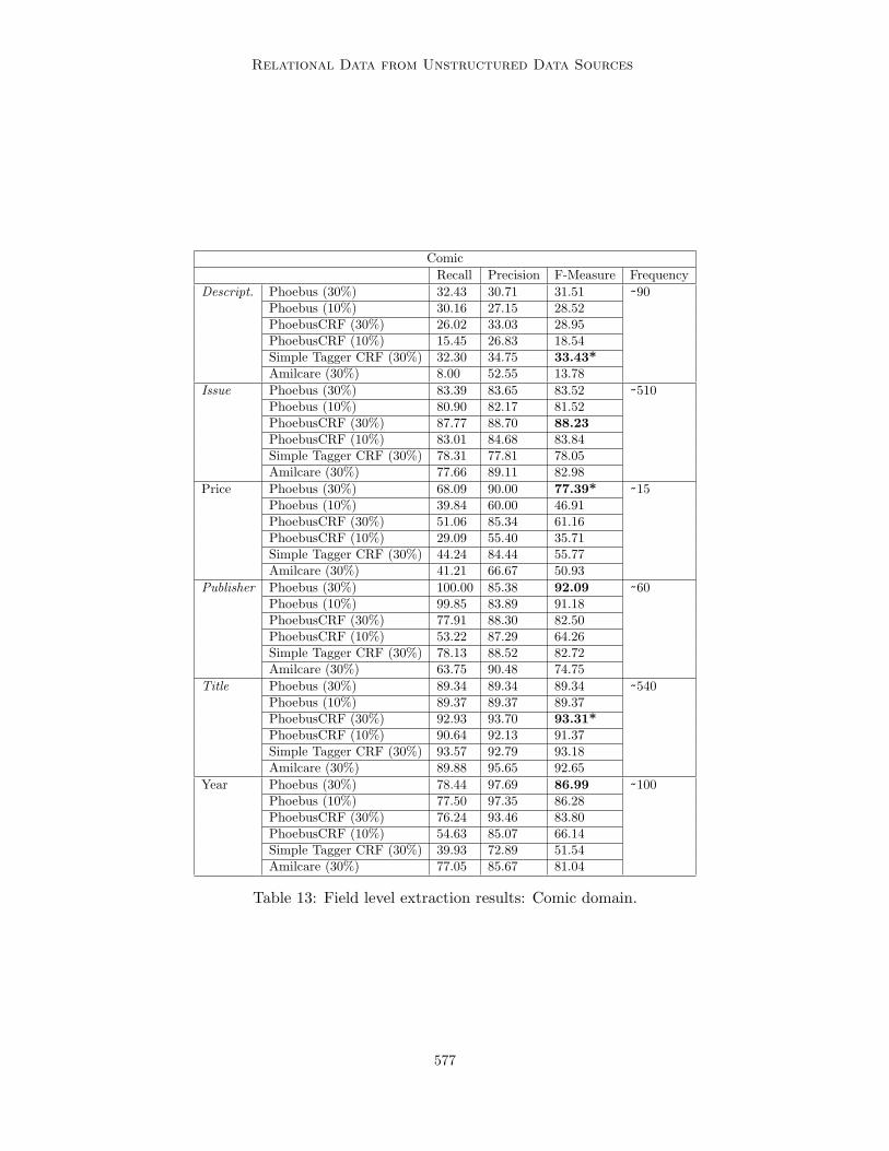
Relational Data from Unstructured Data Sources
ComicRecall Precision F-Measure Frequency
Descript. Phoebus (30%) 32.43 30.71 31.51 ~90Phoebus (10%) 30.16 27.15 28.52PhoebusCRF (30%) 26.02 33.03 28.95PhoebusCRF (10%) 15.45 26.83 18.54Simple Tagger CRF (30%) 32.30 34.75 33.43*Amilcare (30%) 8.00 52.55 13.78
Issue Phoebus (30%) 83.39 83.65 83.52 ~510Phoebus (10%) 80.90 82.17 81.52PhoebusCRF (30%) 87.77 88.70 88.23PhoebusCRF (10%) 83.01 84.68 83.84Simple Tagger CRF (30%) 78.31 77.81 78.05Amilcare (30%) 77.66 89.11 82.98
Price Phoebus (30%) 68.09 90.00 77.39* ~15Phoebus (10%) 39.84 60.00 46.91PhoebusCRF (30%) 51.06 85.34 61.16PhoebusCRF (10%) 29.09 55.40 35.71Simple Tagger CRF (30%) 44.24 84.44 55.77Amilcare (30%) 41.21 66.67 50.93
Publisher Phoebus (30%) 100.00 85.38 92.09 ~60Phoebus (10%) 99.85 83.89 91.18PhoebusCRF (30%) 77.91 88.30 82.50PhoebusCRF (10%) 53.22 87.29 64.26Simple Tagger CRF (30%) 78.13 88.52 82.72Amilcare (30%) 63.75 90.48 74.75
Title Phoebus (30%) 89.34 89.34 89.34 ~540Phoebus (10%) 89.37 89.37 89.37PhoebusCRF (30%) 92.93 93.70 93.31*PhoebusCRF (10%) 90.64 92.13 91.37Simple Tagger CRF (30%) 93.57 92.79 93.18Amilcare (30%) 89.88 95.65 92.65
Year Phoebus (30%) 78.44 97.69 86.99 ~100Phoebus (10%) 77.50 97.35 86.28PhoebusCRF (30%) 76.24 93.46 83.80PhoebusCRF (10%) 54.63 85.07 66.14Simple Tagger CRF (30%) 39.93 72.89 51.54Amilcare (30%) 77.05 85.67 81.04
Table 13: Field level extraction results: Comic domain.
577

Michelson & Knoblock
CarsRecall Precision F-Measure Frequency
Make Phoebus (10%) 98.21 99.93 99.06 ~580PhoebusCRF (10%) 90.73 96.71 93.36Simple Tagger CRF (10%) 85.68 95.69 90.39Amilcare (10%) 97.58 91.76 94.57
Model Phoebus (10%) 92.61 96.67 94.59 ~620PhoebusCRF (10%) 84.58 94.10 88.79Simple Tagger CRF (10%) 78.76 91.21 84.52Amilcare (10%) 78.44 84.31 81.24
Price Phoebus (10%) 97.17 95.91 96.53 ~580PhoebusCRF (10%) 93.59 92.59 93.09Simple Tagger CRF (10%) 83.66 98.16 90.33Amilcare (10%) 90.06 91.27 90.28
Trim Phoebus (10%) 63.11 70.15 66.43 ~375PhoebusCRF (10%) 55.61 64.95 59.28Simple Tagger CRF (10%) 55.94 66.49 60.57Amilcare (10%) 27.21 53.99 35.94
Year Phoebus (10%) 88.48 98.23 93.08 ~600PhoebusCRF (10%) 85.54 96.44 90.59Simple Tagger CRF (10%) 91.12 76.78 83.31Amilcare (10%) 86.32 91.92 88.97
Table 14: Field level extraction results: Cars domain.
Num. of Max. F-MeasuresDomainPhoebus PhoebusCRF Amilcare Simple Tagger
Total Attributes
Hotel 1 3 1 0 5Comic 2 1 0 0 6Cars 5 0 0 0 5All 8 4 1 0 16
Table 15: Summary results for extraction showing the number of times each system hadstatistically significant highest F-Measure for an attribute.
578

Relational Data from Unstructured Data Sources
Phoebus performs especially well in the Cars domain, where it is the best system onall the attributes. One interesting thing to note about this result is that while the recordlinkage results are not spectacular for the Cars domain, they are good enough to yield veryhigh extraction results. This is because most times when the system is not picking the bestmatch from the reference set, it is still picking one that is close enough such that mostof the reference set attributes are useful for extraction. This is why the trim extractionresults are the lowest, because that is often the attribute that determines a match from anon-match. The record linkage step likely selects a car that is close, but differs in the trim,so the match is incorrect and the trim will most likely not be extracted correctly, but therest of the attributes can be extracted using the reference set member.
A couple of other interesting notes come from these results. One of the most intriguingaspects of these results is that they allow us to estimate some level of structure for differentattributes within a domain. Since CRFs rely more on the structure of the tokens withina post than the structured SVM method, we hypothesize that in the domains with morestructure, PhoebusCRF should perform best and in the domains with the least structure,Phoebus should perform best. Table 15 shows this to be the case. PhoebusCRF dominatesthe Hotels domain, where, for example, many posts have a structure where the star ratingcomes before the hotel name. So using such structure should allow the extractor to getthe hotel name more accurately than not using this information. Therefore we see thatoverall there is structure within the Hotels domain because PhoebusCRF is the methodthat performs best, not Phoebus. Contrast this with the Cars domain, which is highlyunstructured, where Phoebus performs the best across all attributes. In this domain thereare many missing tokens and the order of attributes is more varied. The Comic domain isvaried with both some attributes that exhibit structure and some that do not, and as Table15 shows, so are the cases where Phoebus or PhoebusCRF dominates. However, althoughthe Hotels data exhibits some structure, the important aspect of this research is that usingPhoebus allows one to perform extraction without assuming any structure in the data.
Also, a result worth noting is that the price attribute in the Comic domain is a bitmisleading. In fact, none of the systems were statistically significant with respect to eachother because there were so few prices to extract that the F-Measures were all over for allthe systems.
Another aspect that came to light with statistical significance is the generalization of thealgorithm. For the Hotels and Comic domains, where we were able to use both 30% and 10%of the data for training, there are not many cases with a statistically significant differencein the F-Measures for the extracted attributes using Phoebus. In the Hotels domain thename, the area and date had statistically significant F-Measures between training on 30%and 10% of the data, and in the Comic domain only the difference in F-Measure between theissue and description attributes were significant (though the description was borderline).This means of the 11 attributes in both domains, roughly half of them were insignificant.Therefore there is little difference in extraction whether we use 10% of the data for trainingor 30%, so the extraction algorithm generalizes very well. This is important since labelingdata for extraction is very time consuming and expensive.
One interesting result to note is that except for the comic price (which was insignificantfor all systems) and the hotel date (which was close), Phoebus, using either 10% or 30%training data, outperformed all of the other systems on the attributes that were not included
579

Michelson & Knoblock
in the reference set. This lends credibility to our claim earlier in the section that by trainingthe system to extract all of the attributes, even those in the reference set, we can moreaccurately extract attributes not in the reference set because we are training the system toidentify what something is not.
The overall performance of Phoebus validates this approach to semantic annotation. Byinfusing information extraction with the outside knowledge of reference sets, Phoebus isable to perform well across three different domains, each representative of a different typeof source of posts: the auction sites, Internet classifieds and forum/bulletin boards.
5. Discussion
The goal of this research is to produce relational data from unstructured and ungrammaticaldata sources so that they can be accurately queried and integrated with other sources. Byrepresenting the attributes embedded within a post with the standardized values from thereference set, we can support structural queries and integration. For instance, we canperform aggregate queries because we can treat the data source as a relational databasenow. Furthermore, we have standardized values for performing joins across data sources,a key for integration of multiple sources. These standardized values also aid in the caseswhere the post actually does not contain the attribute. For instance, in Table 1, two ofthe listings do not include the make “Honda.” However, once matched to the reference set,they contain a standardized value for this attribute which can then be used for querying andintegrating these posts. This is especially powerful since the posts never explicitly statedthese attribute values. The reference set attributes also provide a solution for the caseswhere the extraction is extremely difficult. For example, none of the systems extractedthe description attribute of the Comic domain well. However, if one instead considersthe description attribute from the reference set, which is quantified by the record linkageresults for the Comic domain, this yields an improvement of over 50% in the F-Measure foridentifying the description for a post.
It may seem that using the reference set attributes for annotation is enough since thevalues are already cleaned, and that extraction is unnecessary. However, this is not the case.For one thing, one may want to see the actual values entered for different attributes. Forinstance, a user might want to discover the most common spelling mistake or abbreviationfor a attribute. Also, there are cases when the extraction results outperform the recordlinkage results. This happens because even if a post is matched to an incorrect member ofthe reference set, that incorrect member is most likely very close to the correct match, andso it can be used to correctly extract much of the information. For a strong example of this,consider the Cars domain. The F-measure for the record linkage results are not as good asthose for the extraction results in this domain. This means most matches that were chosenwhere probably incorrect because they differ from the correct match by something small.For example, a true match could have the trim as “2 Door” while the incorrectly chosenmatch might have the trim “4 Door,” but there would still be enough information, such asthe rest of the trim tokens, the year, the make and the model to correctly extract thosedifferent attributes from the post itself. By performing the extraction for the values fromthe post itself, we can overcome the mistakes of the record linkage step because we can stillexploit most of the information in the incorrectly chosen reference set member.
580

Relational Data from Unstructured Data Sources
Extraction on all of the attributes also helps our system classify (and ignore) “junk”tokens. Labeling something as junk is much more descriptive if it is labeled junk out ofmany possible class labels that could share lexical characteristics. This helps improve theextraction results on items that are not in the reference set, such as prices and dates.
On the topic of reference sets, it is important to note that the algorithm is not tied toa single reference set. The algorithm extends to include multiple reference sets by iteratingthe process for each reference set used.
Consider the following two cases. First, suppose a user wants to extract conferencenames and cities and she has individual lists of each. If the approach is confined to usingone reference set, that would require constructing a reference set that contains the power setof cities crossed with conference names. This approach would not scale for many attributesfrom distinct sources. However, if these lists are used as two reference sets, one for eachattribute, the algorithm can run once with the conference name data, and once with areference set of cities. This iterative exploitation of the reference sets allows for n referenceset attributes to be added without a combinatorial explosion.
The next interesting case is when a post contains more than one of the same attribute.For example, a user needs to extract two cities from some post. If one reference set is used,then it includes the cross product of all cities. However, using a single reference set of citynames can be done by slightly modifying the algorithm. The new algorithm makes a firstpass with the city reference set. During this pass, the record linkage match will either beone of the cities that matches best, or a tie between them. In the case of a tie, choose thefirst match. Using this reference city, our system can then extract the city from the post,and remove it from the post. Then our system simply runs the process again, which willcatch the second city, using the same, single reference set. This could be repeated as manytimes as needed.
One issue that arises with reference sets is the discrepancy between user’s knowledgeand the domain experts who generally create the reference sets. In the Cars domain, forinstance, users will interchangeably use the attribute values “hatchback,” “liftback,” and“wagon.” The reference set never includes the term “liftback” which suggests it is a synonymfor hatchback used in common speech, but not in Edmund’s automobile jargon. The term“wagon” is used by Edmunds, but it is not used for some of the cars that users describeas “hatchbacks.” This implies a slight difference in meaning between the two, according tothe reference set authors.
Two issues arise from these discrepancies. The first is the users interchanging the wordscan cause some problems for the extraction and for the record linkage, but this can beovercome by incorporating some sort of thesaurus into the algorithm. During record linkage,a thesaurus could expand certain attribute values used for matching, for example including“hatchback” and “liftback” when the reference set attribute includes the term “wagon.”However, there are more subtle issues here. It is mostly not the case that a “hatchback” iscalled a “wagon” but it does happen that a “wagon” is called a “hatchback.” The frequencyof replacement must be taken into consideration so that errant matches are not created.How to automate this is a line of future research. The other issue arises from trustingthe correctness of the Edmunds source. We assume Edmunds is right to define one caras a “wagon” which has a different meaning from classifying it as a “hatchback.” In fact,
581
Michelson & Knoblock
Edmunds classifies the Mazda Protege5 as a “wagon,” while Kelly Blue Book16 classifies itas a “hatchback.” This seems to invalidate the idea that “wagon” is different in meaningfrom “hatchback.” They appear to be simple synonyms, but this would remain unknownwithout the outside knowledge of Kelly Blue Book. More generally, one assumes that thereference set is a correct set of standardized values, but this is not an absolute truth. That iswhy the most meaningful reference sets are those that can be constructed from agreed-uponontologies from the Semantic Web. For instance, a reference set derived from an ontologyfor cars created by all of the biggest automotive businesses should alleviate many of theissues in meaning, and a thesaurus scheme could work out the discrepancies introduced bythe users, rather than the reference sets.
6. Related Work
Our research is driven by the principal that the cost of annotating documents for theSemantic Web should be free, that is, automatic and invisible to users (Hendler, 2001).Many researchers have followed this path, attempting to automatically mark up documentsfor the Semantic Web, as proposed here (Cimiano, Handschuh, & Staab, 2004; Dingli,Ciravegna, & Wilks, 2003; Handschuh, Staab, & Ciravegna, 2002; Vargas-Vera, Motta,Domingue, Lanzoni, Stutt, & Ciravegna, 2002). However, these systems rely on lexicalinformation, such as part-of-speech tagging or shallow Natural Language Processing to dotheir extraction/annotation (e.g., Amilcare, Ciravegna, 2001). This is not an option whenthe data is ungrammatical, like the post data. In a similar vein, there are systems such asADEL (Lerman, Gazen, Minton, & Knoblock, 2004) which rely on the structure to identifyand annotate records in Web pages. Again, the failure of the posts to exhibit structuremakes this approach inappropriate. So, while there is a fair amount of work in automaticlabeling, there is little emphasis on techniques that could label text that is both unstructuredand ungrammatical.
Although the idea of record linkage is not new (Fellegi & Sunter, 1969) and is well studiedeven now (Bilenko & Mooney, 2003) most current research focuses on matching one set ofrecords to another set of records based on their decomposed attributes. There is little workon matching data sets where one record is a single string composed of the other data set’sattributes to match on, as in the case with posts and reference sets. The WHIRL system(Cohen, 2000) allows for record linkage without decomposed attributes, but as shown inSection 4.1 Phoebus outperforms WHIRL, since WHIRL relies solely on the vector-basedcosine similarity between the attributes, while Phoebus exploits a larger set of features torepresent both field and record level similarity. We note with interest the EROCS system(Chakaravarthy, Gupta, Roy, & Mohania, 2006) where the authors tackle the problem oflinking full text documents with relational databases. The technique involves filtering outall non-nouns from the text, and then finding the matches in the database. This is anintriguing approach; interesting future work would involve performing a similar filtering forlarger documents and then applying the Phoebus algorithm to match the remaining nounsto reference sets.
Using the reference set’s attributes as normalized values is similar to the idea of datacleaning. However, most data cleaning algorithms assume tuple-to-tuple transformations
16. www.kbb.com
582

Relational Data from Unstructured Data Sources
(Lee et al., 1999; Chaudhuri et al., 2003). That is, some function maps the attributes ofone tuple to the attributes of another. This approach would not work on ungrammaticaland unstructured data, where all attributes are embedded within the post, which maps toa set of attributes from the reference set.
Although our work describes a technique for information extraction, many methods,such as Conditional Random Fields (CRF), assume at least some structure in the extractedattributes to do the extraction. As our extraction experiments show, Phoebus outper-forms such methods, such as the Simple Tagger implementation of Conditional RandomFields (McCallum, 2002). Other IE approaches, such as Datamold (Borkar, Deshmukh, &Sarawagi, 2001) and CRAM (Agichtein & Ganti, 2004), segment whole records (like bib-liographies) into attributes, with little structural assumption. In fact, CRAM even usesreference sets to aid its extraction. However, both systems require that every token of arecord receive a label, which is not possible with posts that are filled with irrelevant, “junk”tokens. Along the lines of CRAM and Datamold, the work of Bellare and McCallum (2007)uses a reference set to train a CRF to extract data, which is similar to our PhoebusCRFimplementation. However, there are two differences between PhoebusCRF and their work(Bellare & McCallum, 2007). First, the work of Bellare and McCallum (2007) mentionsthat reference set records are matched using simple heuristics, but it is unclear how this isdone. In our work, matching is done explicitly and accurately through record linkage. Sec-ond, their work only uses the records from the reference set to label tokens for training anextraction module, while PhoebusCRF uses the actual values from the matching referenceset record to produce useful features for extraction and annotation.
Another IE approach similar to ours performs named entity recognition using “Semi-CRFs” with a dictionary component (Cohen & Sarawagi, 2004), which functions like areference set. However, in their work the dictionaries are defined as lists of single attributeentities, so finding an entity in the dictionary is a look-up task. Our reference sets arerelational data, so finding the match becomes a record linkage task. Further, their work onSemi-CRFs (Cohen & Sarawagi, 2004) focuses on the task of labeling segments of tokenswith a uniform label, which is especially useful for named entity recognition. In the caseof posts, however, Phoebus needs to relax such a restriction because in some cases suchsegments will be interrupted, as the case of a hotel name with the area in the middle ofthe hotel name segment. So, unlike their work, Phoebus makes no assumptions about thestructure of posts. Recently, Semi-CRFs have been extended to use database records in thetask of integrating unstructured data with relational databases (Mansuri & Sarawagi, 2006).This work is similar to ours in that it links unstructured data, such as paper citations, withrelational databases, such as reference sets of authors and venues. The difference is that weview this as a record linkage task, namely finding the right reference set tuple to match. Intheir paper, even though they use matches from the database to aid extraction, they viewthe linkage task as an extraction procedure followed by a matching task. Lastly, we arenot the first to consider structured SVMs for information extraction. Previous work usedstructured SVMs to perform Named Entity Recognition (Tsochantaridis et al., 2005) buttheir extraction task does not use reference sets.
Our method of aiding information extraction with outside information (in the form ofreference sets) is similar to the work on ontology-based information extraction (Embley,Campbell, Jiang, Liddle, Ng, Quass, & Smith, 1999). Later versions of their work even talk
583
Michelson & Knoblock
about using ontology-based information extraction as a means to semantically annotate un-structured data such as car classifieds (Ding, Embley, & Liddle, 2006). However, in contrastto our work, the information extraction is performed by a keyword-lookup into the ontologyalong with structural and contextual rules to aid the labeling. The ontology itself containskeyword misspellings and abbreviations, so that the look-up can be performed in the pres-ence of noisy data. We believe the ontology-based extraction approach is less scalable thana record linkage type matching task because creating and maintaining the ontology requiresextensive data engineering in order to encompass all possible common spelling mistakes andabbreviations. Further, if new data is added to the ontology, additional data engineeringmust be performed. In our work, we can simply add new tuples to our reference set. Lastly,in contrast to our work, this ontology based work assumes contextual and structural ruleswill apply, making an assumption about the data to extract from. In our work, we makeno such assumptions about the structure of the text we are extracting from.
Yet another interesting approach to information extraction using ontologies is the Text-presso system which extracts data from biological text (Muller & Sternberg, 2004). Thissystem uses a regular expression based keyword look-up to label tokens in some text basedon the ontology. Once all tokens are labeled, Textpresso can perform “fact extraction”by extracting sequences of labeled tokens that fit a particular pattern, such as gene-allelereference associations. Although this system again uses a reference set for extraction, itdiffers in that it does a keyword look-up into the lexicon.
In recent work on learning efficient blocking schemes Bilenko et al., (2006) developed asystem for learning disjunctive normal form blocking schemes. However, they learn theirschemes using a graphical set covering algorithm, while we use a version of the SequentialCovering Algorithm (SCA). There are also similarities between our BSL algorithm and workon mining association rules from transaction data (Agrawal, Imielinski, & Swami, 1993).Both algorithms discover propositional rules. Further, both algorithms use multiple passesover a data set to discover their rules. However despite these similarities, the techniquesreally solve different problems. BSL generates a set of candidate matches with a minimalnumber of false positives. To do this, BSL learns conjunctions that are maximally specific(eliminating many false positives) and unions them together as a single disjunctive rule (tocover the different true positives). Since the conjunctions are maximally specific, BSL usesSCA underneath, which learns rules in a depth-first, general to specific manner (Mitchell,1997). On the other hand, the work of mining association rules (Agrawal et al., 1993) looksfor actual patterns in the data that represent some internal relationships. There may bemany such relationships in the data that could be discovered, so this approach covers thedata in a breadth-first fashion, selecting the set of rules at each iteration and extendingthem by appending to each a new possible item.
7. Conclusion
This article presents an algorithm for semantically annotating text that is ungrammaticaland unstructured. Unstructured, ungrammatical sources contain much information, butcannot support structured queries. Our technique allows for more informative use of thesources. Using our approach, eBay agents could monitor the auctions looking for the bestdeals, or a user could find the average price of a four-star hotel in San Diego. Such semantic
584

Relational Data from Unstructured Data Sources
annotation is necessary as society transitions into the Semantic Web, where informationrequires annotation to be useful for agents, but users are unwilling to do the extra work toprovide the required annotation.
In the future, our technique could link with a mediator framework (Thakkar, Ambite, &Knoblock, 2004) for automatically acquiring reference sets. This is similar to automaticallyincorporating secondary sources for record linkage (Michalowski, Thakkar, & Knoblock,2005). The automatic formulation of queries to retrieve the correct domain reference setis a direction of future research. With a mediator framework in place, Phoebus couldincorporate as many reference sets as needed for full coverage of possible attribute valuesand attribute types.
Unsupervised approaches to record linkage and extraction are also topics of future re-search. By including unsupervised record linkage and extraction with a mediator compo-nent, the approach would be entirely self-contained, making semantic annotation of postsa more automatic process. Also, the current implementation only gives one class label pertoken. Ideally Phoebus would give a token all possible labels, and then remove the ex-traneous tokens when the systems cleans the attributes, as described in Section 3. Thisdisambiguation should lead to much higher accuracy during extraction.
Future work could investigate the inclusion of thesauri for terms in the attributes, withthe frequency of replacement of the terms taken into consideration. Also, exploring tech-nologies that automatically construct the reference sets (and eventually thesauri) from thenumerous ontologies on the Semantic Web is an intriguing research path.
The long term goal for annotation and extraction from unstructured, ungrammaticalsources involves automating the entire process. If the record linkage and extraction methodscould become unsupervised, then our approach could automatically generate and incorpo-rate the reference sets, and then apply them to automatically annotate the data source.This would be an ideal approach for making the Semantic Web more useful – with no userinvolvement.
Acknowledgments
This research is based upon work supported in part by the National Science Foundation un-der award number IIS-0324955, in part by the Air Force Office of Scientific Research undergrant number FA9550-07-1-0416, and in part by the Defense Advanced Research ProjectsAgency (DARPA), through the Department of the Interior, NBC, Acquisition Services Di-vision, under Contract No. NBCHD030010.
The U.S.Government is authorized to reproduce and distribute reports for Governmen-tal purposes notwithstanding any copyright annotation thereon. The views and conclusionscontained herein are those of the authors and should not be interpreted as necessarily rep-resenting the official policies or endorsements, either expressed or implied, of any of theabove organizations or any person connected with them.
585

Michelson & Knoblock
References
Agichtein, E., & Ganti, V. (2004). Mining reference tables for automatic text segmentation.In the Proceedings of the 10th ACM Conference on Knowledge Discovery and DataMining, pp. 20 – 29. ACM Press.
Agrawal, R., Imielinski, T., & Swami, A. (1993). Mining association rules between sets ofitems in large databases. In Proceedings of the ACM SIGMOD International Confer-ence on Management of Data, pp. 207–216. ACM Press.
Baxter, R., Christen, P., & Churches, T. (2003). A comparison of fast blocking methods forrecord linkage. In Proceedings of the 9th ACM SIGKDD Workshop on Data Cleaning,Record Linkage, and Object Identification, pp. 25–27.
Bellare, K., & McCallum, A. (2007). Learning extractors from unlabeled text using relevantdatabases. In Proceedings of the AAAI Workshop on Information Integration on theWeb, pp. 10–16.
Bilenko, M., Kamath, B., & Mooney, R. J. (2006). Adaptive blocking: Learning to scale uprecord linkage and clustering. In Proceedings of the 6th IEEE International Conferenceon Data Mining, pp. 87–96.
Bilenko, M., & Mooney, R. J. (2003). Adaptive duplicate detection using learnable stringsimilarity measures. In Proceedings of the 9th ACM International Conference onKnowledge Discovery and Data Mining, pp. 39–48. ACM Press.
Borkar, V., Deshmukh, K., & Sarawagi, S. (2001). Automatic segmentation of text intostructured records. In Proceedings of the ACM SIGMOD International Conference onManagement of Data, pp. 175–186. ACM Press.
Califf, M. E., & Mooney, R. J. (1999). Relational learning of pattern-match rules forinformation extraction. In Proceedings of the 16th National Conference on ArtificialIntelligence, pp. 328–334.
Chakaravarthy, V. T., Gupta, H., Roy, P., & Mohania, M. (2006). Efficiently linking textdocuments with relevant structured information. In Proceedings of the InternationalConference on Very Large Data Bases, pp. 667–678. VLDB Endowment.
Chaudhuri, S., Ganjam, K., Ganti, V., & Motwani, R. (2003). Robust and efficient fuzzymatch for online data cleaning. In Proceedings of ACM SIGMOD International Con-ference on Management of Data, pp. 313–324. ACM Press.
Cimiano, P., Handschuh, S., & Staab, S. (2004). Towards the self-annotating web. InProceedings of the 13th International Conference on World Wide Web, pp. 462–471.ACM Press.
Ciravegna, F. (2001). Adaptive information extraction from text by rule induction andgeneralisation.. In Proceedings of the 17th International Joint Conference on ArtificialIntelligence, pp. 1251–1256.
586
Relational Data from Unstructured Data Sources
Cohen, W., & Sarawagi, S. (2004). Exploiting dictionaries in named entity extraction: com-bining semi-markov extraction processes and data integration methods. In Proceedingsof the 10th ACM International Conference on Knowledge Discovery and Data Mining,pp. 89–98, Seattle, Washington. ACM Press.
Cohen, W. W. (2000). Data integration using similarity joins and a word-based informationrepresentation language. ACM Transactions on Information Systems, 18 (3), 288–321.
Cohen, W. W., Ravikumar, P., & Feinberg, S. E. (2003). A comparison of string metricsfor matching names and records. In Proceedings of the ACM SIGKDD Workshop onData Cleaning, Record Linkage, and Object Consoliation, pp. 13–18.
Crescenzi, V., Mecca, G., & Merialdo, P. (2001). Roadrunner: Towards automatic dataextraction from large web sites. In Proceedings of 27th International Conference onVery Large Data Bases, pp. 109–118. VLDB Endowment.
Ding, Y., Embley, D. W., & Liddle, S. W. (2006). Automatic creation and simplified query-ing of semantic web content: An approach based on information-extraction ontologies.In Proceedings of the Asian Semantic Web Conference, pp. 400–414.
Dingli, A., Ciravegna, F., & Wilks, Y. (2003). Automatic semantic annotation using unsu-pervised information extraction and integration. In Proceedings of the K-CAP Work-shop on Knowledge Markup and Semantic Annotation.
Elfeky, M. G., Verykios, V. S., & Elmagarmid, A. K. (2002). TAILOR: A record linkagetoolbox. In Proceedings of 18th International Conference on Data Engineering, pp.17–28.
Embley, D. W., Campbell, D. M., Jiang, Y. S., Liddle, S. W., Ng, Y.-K., Quass, D., &Smith, R. D. (1999). Conceptual-model-based data extraction from multiple-recordweb pages. Data Knowledge Engineering, 31 (3), 227–251.
Fellegi, I. P., & Sunter, A. B. (1969). A theory for record linkage. Journal of the AmericanStatistical Association, 64, 1183–1210.
Handschuh, S., Staab, S., & Ciravegna, F. (2002). S-cream - semi-automatic creation ofmetadata. In Proceedings of the 13th International Conference on Knowledge Engi-neering and Knowledge Management, pp. 165–184. Springer Verlag.
Hendler, J. (2001). Agents and the semantic web. IEEE Intelligent Systems, 16 (2), 30–37.
Hernandez, M. A., & Stolfo, S. J. (1998). Real-world data is dirty: Data cleansing and themerge/purge problem. Data Mining and Knowledge Discovery, 2 (1), 9–37.
Jaro, M. A. (1989). Advances in record-linkage methodology as applied to matching the1985 census of tampa, florida. Journal of the American Statistical Association, 89,414–420.
Joachims, T. (1999). Advances in Kernel Methods - Support Vector Learning, chap. 11:Making large-Scale SVM Learning Practical. MIT-Press.
587

Michelson & Knoblock
Lafferty, J., McCallum, A., & Pereira, F. (2001). Conditional random fields: Probabilis-tic models for segmenting and labeling sequence data. In Proceedings of the 18thInternational Conference on Machine Learning, pp. 282–289. Morgan Kaufmann.
Lee, M.-L., Ling, T. W., Lu, H., & Ko, Y. T. (1999). Cleansing data for mining andwarehousing. In Proceedings of the 10th International Conference on Database andExpert Systems Applications, pp. 751–760. Springer-Verlag.
Lerman, K., Gazen, C., Minton, S., & Knoblock, C. A. (2004). Populating the semantic web.In Proceedings of the AAAI Workshop on Advances in Text Extraction and Mining.
Levenshtein, V. I. (1966). Binary codes capable of correcting deletions, insertions, andreversals. English translation in Soviet Physics Doklady, 10 (8), 707–710.
Mansuri, I. R., & Sarawagi, S. (2006). Integrating unstructured data into relationaldatabases. In Proceedings of the International Conference on Data Engineering, p. 29.IEEE Computer Society.
McCallum, A. (2002). Mallet: A machine learning for language toolkit.http://mallet.cs.umass.edu.
McCallum, A., Nigam, K., & Ungar, L. H. (2000). Efficient clustering of high-dimensionaldata sets with application to reference matching. In Proceedings of the 6th ACMSIGKDD, pp. 169–178.
Michalowski, M., Thakkar, S., & Knoblock, C. A. (2005). Automatically utilizing secondarysources to align information across sources. In AI Magazine, Special Issue on SemanticIntegration, Vol. 26, pp. 33–45.
Michelson, M., & Knoblock, C. A. (2005). Semantic annotation of unstructured and ungram-matical text. In Proceedings of the 19th International Joint Conference on ArtificialIntelligence, pp. 1091–1098.
Michelson, M., & Knoblock, C. A. (2006). Learning blocking schemes for record linkage. InProceedings of the 21st National Conference on Artificial Intelligence.
Michelson, M., & Knoblock, C. A. (2007). Unsupervised information extraction from un-structured, ungrammatical data sources on the world wide web. International Journalof Document Analysis and Recognition (IJDAR), Special Issue on Noisy Text Analyt-ics.
Mitchell, T. M. (1997). Machine Learning. McGraw-Hill, New York.
Muller, H.-M., & Sternberg, E. E. K. P. W. (2004). Textpresso: An ontology-based infor-mation retrieval and extraction system for biological literature. PLoS Biology, 2 (11).
Muslea, I., Minton, S., & Knoblock, C. A. (2001). Hierarchical wrapper induction forsemistructured information sources. Autonomous Agents and Multi-Agent Systems,4 (1/2), 93–114.
588

Relational Data from Unstructured Data Sources
Newcombe, H. B. (1967). Record linkage: The design of efficient systems for linking recordsinto individual and family histories. American Journal of Human Genetics, 19 (3),335–359.
Porter, M. F. (1980). An algorithm for suffix stripping. Program, 14 (3), 130–137.
Smith, T. F., & Waterman, M. S. (1981). Identification of common molecular subsequences.Journal of Molecular Biology, 147, 195–197.
Soderland, S. (1999). Learning information extraction rules for semi-structured and freetext. Machine Learning, 34 (1-3), 233–272.
Thakkar, S., Ambite, J. L., & Knoblock, C. A. (2004). A data integration approach toautomatically composing and optimizing web services. In Proceedings of the ICAPSWorkshop on Planning and Scheduling for Web and Grid Services.
Tsochantaridis, I., Hofmann, T., Joachims, T., & Altun, Y. (2004). Support vector machinelearning for interdependent and structured output spaces. In Proceedings of the 21stInternational Conference on Machine Learning, p. 104. ACM Press.
Tsochantaridis, I., Joachims, T., Hofmann, T., & Altun, Y. (2005). Large margin methodsfor structured and interdependent output variables. Journal of Machine LearningResearch, 6, 1453–1484.
Vargas-Vera, M., Motta, E., Domingue, J., Lanzoni, M., Stutt, A., & Ciravegna, F. (2002).MnM: Ontology driven semi-automatic and automatic support for semantic markup.In Proceedings of the 13th International Conference on Knowledge Engineering andManagement, pp. 213–221.
Wellner, B., McCallum, A., Peng, F., & Hay, M. (2004). An integrated, conditional modelof information extraction and coreference with application to citation matching. InProceedings of the 20th Conference on Uncertainty in Artificial Intelligence, pp. 593–601.
Winkler, W. E., & Thibaudeau, Y. (1991). An application of the fellegi-sunter model ofrecord linkage to the 1990 U.S. Decennial Census. Tech. rep., Statistical ResearchReport Series RR91/09 U.S. Bureau of the Census.
Zhai, C., & Lafferty, J. (2001). A study of smoothing methods for language models appliedto ad hoc information retrieval. In Proceedings of the 24th ACM SIGIR Conferenceon Research and Development in Information Retrieval, pp. 334–342. ACM Press.
589