creating digital environments for multi-agent simulation
TRANSCRIPT

Calhoun: The NPS Institutional Archive
Theses and Dissertations Thesis and Dissertation Collection
2003-12
Creating digital environments for multi-agent simulation
Tanner, Mark B.
Monterey, California. Naval Postgraduate School
http://hdl.handle.net/10945/6129

MONTEREY, CALIFORNIA
THESIS CREATING DIGITAL ENVIRONMENTS FOR MULTI-AGENT
SIMULATION
by
Mark B. Tanner
December 2003
Thesis Advisor: Wolfgang Baer Thesis Co-Advisor: David W. Laflam
This thesis done in cooperation with the MOVES institute.
Approved for public release; distribution is unlimited.

REPORT DOCUMENTATION PAGE Form Approved OMB No. 0704-0188
Public reporting burden for this collection of information is estimated to average 1 hour per response, including the time for reviewing instruction, searching existing data sources, gathering and maintaining the data needed, and completing and reviewing the collection of information. Send comments regarding this burden estimate or any other aspect of this collection of information, including suggestions for reducing this burden, to Washington headquarters Services, Directorate for Information Operations and Reports, 1215 Jefferson Davis Highway, Suite 1204, Arlington, VA 22202-4302, and to the Office of Management and Budget, Paperwork Reduction Project (0704-0188) Washington DC 20503. 1. AGENCY USE ONLY (Leave blank)
2. REPORT DATE December 2003
3. REPORT TYPE AND DATES COVERED Master’s Thesis
4. TITLE AND SUBTITLE Creating Di l Environments for Multi-Agent Simulation gita
5. FUNDING NUMBERS
6. AUTHOR Mark B. Tanner 7. PERFORMING ORGANIZATION NAME(S) AND ADDRESS(ES) Naval Postgraduate School Monterey, CA 93943-5000
8. PERFORMING ORGANIZATION REPORT NUMBER
9. SPONSORING / MONITORING AGENCY NAME(S) AND ADDRESS(ES) 10. SPONSORING / MONITORING AGENCY REPORT NUMBER
11. SUPPLEMENTARY NOTES The views expressed in this thesis are those of the author and do not reflect the official policy or position of the Department of Defense or the U.S. Government. 12a. DISTRIBUTION / AVAILABILITY STATEMENT Approved for public release; distribution is unlimited.
12b. DISTRIBUTION CODE
13. ABSTRACT (maximum 200 words) There are few tools available for military and civilian simulation developers to quickly and efficiently develop high-fidelity
digital environments capable of supporting high-resolution, agent-based simulation. In this work, the author has tried to lay a solid
foundation for further understanding the digital terrain support available to simulation developers.
This thesis explores numerous digital terrain data representations and tools available to create digital environments. The work
explores the specific problem of terrain database generation for agent-based ground combat simulation. To accomplish this, the author
explores the more general problem of where to find the data, what tools are available, and how to put the pieces together to create a
registered digital environment on a state-of-the-art computer. The author envisions this methodology to be the first step in the design
of an automated planning tool capable of importing real world digital terrain data and quickly generating agent-based military combat
scenarios for any location on earth.
This work provides a logical construct and design methodology for an analyst to create high fidelity terrain data sets. It
functions as a “how to” manual to help analysts understand which information and tools are available to use for different types of
simulation projects. 14. SUBJECT TERMS Synthetic Natural Environment, Terrain Data Representation, Terrain Data Format, Agent Based Modeling, Multi-Agent Systems, Complex Adaptive Systems
15. NUMBER OF PAGES 95
16. PRICE CODE 17. SECURITY CLASSIFICATION OF REPORT Unclassified
18. SECURITY CLASSIFICATION OF THIS PAGE Unclassified
19. SECURITY CLASSIFI- CATION OF ABSTRACT Unclassified
20. LIMITATION OF ABSTRACT UL
NSN 7540-01-280-5500 Standard Form 298 (Rev. 2-89) Prescribed by ANSI Std. 239-18
i

THIS PAGE INTENTIONALLY LEFT BLANK
ii
Approved for public release; distribution is unlimited
CREATING DIGITAL ENVIRONMENTS FOR MULTI-AGENT SIMULATION
Mark B. Tanner Major, United States Army
B.S., University of Arizona, 1988 M.S., Chapman University, 1992
Submitted in partial fulfillment of the requirements for the degree of
MASTER OF SCIENCE IN MODELING, VIRTUAL ENVIRONMENTS, AND SIMULATION
from the
NAVAL POSTGRADUATE SCHOOL
December 2003
Author:
Mark B. Tanner
Approved by: Wolfgang Baer Thesis Advisor
David W. Laflam Thesis Co-Advisor
Dr. Rudolph P. Darken MOVES Academic Committee Chair
iii

THIS PAGE INTENTIONALLY LEFT BLANK
iv

ABSTRACT
There are few tools available for military and civilian simulation developers to
quickly and efficiently develop high-fidelity digital environments capable of supporting
high-resolution, agent-based simulation. In this work, the author has tried to lay a solid
foundation for further understanding the digital terrain support available to simulation
developers.
This thesis explores numerous digital terrain data representations and tools
available to create digital environments. The work explores the specific problem of
terrain database generation for agent-based ground combat simulation. To accomplish
this, the author explores the more general problem of where to find the data, what tools
are available, and how to put the pieces together to create a registered digital environment
on a state-of-the-art computer. The author envisions this methodology to be the first step
in the design of an automated planning tool capable of importing real world digital terrain
data and quickly generating agent-based military combat scenarios for any location on
earth.
This work provides a logical construct and design methodology for an analyst to
create high fidelity terrain data sets. It functions as a “how to” manual to help analysts
understand which information and tools are available to use for different types of
simulation projects.
v

THIS PAGE INTENTIONALLY LEFT BLANK
vi

TABLE OF CONTENTS
I. INTRODUCTION .......................................................................................... 1 A. THESIS STATEMENT .............................................................................. 1 B. MOTIVATION........................................................................................... 1 C. GOALS ....................................................................................................... 1 D. ORGANIZATION ...................................................................................... 2
II. BACKGROUND AND RELATED WORK .................................................. 5 A. PARTS OF A GROUND COMBAT SIMULATION................................ 5 B. DATA INTEROPERABILITY .................................................................. 7 C. ADAPTIVE AND AUTONOMOUS MULTI-AGENT SYSTEMS.......... 8 D. IRREDUCIBLE SEMI-AUTONOMOUS ADAPTIVE COMBAT………9
III. DATA REPRESENTATIONS .................................................................... 15 A. INTRODUCTION .................................................................................... 15 B. TERRAIN REPRESENTATIONS ........................................................... 15
1. Gridded Representations....................................................................... 15 a. Digital Terrain Elevation Data (DTED)........................................... 16 b. Digital Elevation Model (DEM) ....................................................... 17
2. Raster Representations.......................................................................... 18 a. ARC Digitized Raster Graphics (ADRG).......................................... 19 b. Compressed ARC Digitized Raster Graphics (CADRG) .................. 20
3. Vector Representations ......................................................................... 21 4. Imagery Representations....................................................................... 22 5. Other Popular Representations ............................................................. 23
a. Global 30-Arc-Second Elevation Data Set (GTOPO30) ................. 23 b. Triangular Irregular Network (TIN) Data........................................ 24
6. Data Representation Analysis .............................................................. 25 7. Ordering Common Terrain Products .................................................... 26
C. DATA FORMATS.................................................................................... 27 1. Vector Product Format (VPF)............................................................... 27 2. Raster Product Format (RPF)................................................................ 28 3. National Imagery Transmission Format Standard (NITFS) ................. 29
D. DEVELOPMENT OF COMMON DATA MODELS.............................. 29 1. Environmental Database Integrated Product Team (EDBIPT)............. 30 2. SEDRIS................................................................................................. 31
IV. TERRAIN MANIPULATION TOOLS....................................................... 35 A. INTRODUCTION .................................................................................... 35 B. ANALYTICAL METHOD....................................................................... 35
1. Cost ....................................................................................................... 35 2. Manufacturer......................................................................................... 35 3. System Requirements............................................................................ 36 4. Data In................................................................................................... 36 5. Data Out ................................................................................................ 36 6. System Description ............................................................................... 36 7. Integration with Other Tools................................................................. 36
vii8. What Does it do Better Than Other Tools ............................................ 36

9. Time to Learn........................................................................................ 37 10. Potential Uses ....................................................................................... 37 11. Where to Get a Demo Version ............................................................. 37
C. PRODUCT ANALYSIS ........................................................................... 37 1. SOCETSet – Digital Photogrammetric Software ................................. 37 2. SOCETSim ........................................................................................... 38 3. Falcon View.......................................................................................... 39 4. EdgeViewer........................................................................................... 41 5. TerraTools............................................................................................. 42 6. Sitebuilder 3D ....................................................................................... 43 7. PVNT .................................................................................................... 45 8. ArcGIS .................................................................................................. 46 9. Additional Products .............................................................................. 47
a. Joint Mapping Toolkit (JMTK) ......................................................... 47 b. ArcExplorer....................................................................................... 47 c. OpenMap........................................................................................... 48 d. MapInfo ProViewer .......................................................................... 48 e. ERDAS ViewFinder .......................................................................... 48 f. Geomedia Viewer.............................................................................. 48 g. DLGV32 ............................................................................................ 48 h. MicroDEM / TerraBase II ................................................................ 48
D. FINAL ANALYSIS.................................................................................. 49 E. CONCLUSION......................................................................................... 49
V. APPLIED SUMMARY ................................................................................ 51 VI. FUTURE WORK......................................................................................... 57 VII. CONCLUSION............................................................................................ 59 LIST OF REFERENCES...................................................................................... 61 INITIAL DISTRIBUTION LIST ......................................................................... 65
viii

LIST OF FIGURES
Figure 2-1. Thesis Focus.....................................................................................................7 Figure 2-2. Screen Capture of the ISAAC Simulation .....................................................11 Figure 2-3. Sample Penalty Calculation ...........................................................................12 Figure 2-4. Multi-Agent System Testbed .........................................................................13 Figure 3-1. DTED Level 0-5 Post Spacing.......................................................................16 Figure 3-2. ADRG Chart Coverage ..................................................................................19 Figure 3-3. Inserting Points Into a Triangulated Irregular Network.................................25 Figure 3-4. Data Representation Quick Reference Guide ................................................26 Figure 3-5. VPF Data Structure ........................................................................................28 Figure 3-6. Representation of RPF Directory and File Structure .....................................29 Figure 3-7. Data Representation Types ............................................................................33 Figure 3-8. Data Representation Scale and Resolution ....................................................34 Figure 4-1. Tools Analysis................................................................................................50 Figure 5-1. Data Flow Diagram Example.........................................................................54
ix

THIS PAGE INTENTIONALLY LEFT BLANK
x

LIST OF ACRONYMS
ACT - Advanced Concepts and Technology
ACTD - Advanced Concept Technology Demonstration
ADRG - ARC Digitized Raster Graphics
ADS - Advanced Distributed Simulation
ALSP - Aggregate Level Simulation Protocol
AMSEC - Army Model and Simulation Executive Council
AMSO - Army Modeling and Simulation Office
ANSI - American National Standards Institute
API - Application Programmer Interface
ASCII - American Standard Code for Information Interchange
ASNE - Air and Space Natural Environment
AWACS - Airborne Warning and Control System
BIIF - Binary Imagery Interchange Format
BV - Battlefield Visualization
C3I - Command, Control, Communications, and Intelligence
C4I - Command, Control, Communications, Computers, and Intelligence
C4ISR - C4I Surveillance and Reconnaissance
CADRG - Compressed ARC Digitized Raster Graphics
CAS - Complex Adaptive System
CBS - Corps Battle Simulation
CIB - Controlled Image Base
CIG - Computer Image Generator
xi

CGF - Computer Generated Forces
CMMS - Conceptual Model of the Mission Space
COTS - Commercial Off-The-Shelf
CT - Coordinate Transformation
CTDB - Compact Terrain Data Base
DARPA - Defense Advanced Research Projects Agency
DBGS - Data Base Generation System
DCHUM - Digital Chart Update Manual
DCW - Digital Chart of the World
DEM - Digital Elevation Model
DFAD - Digital Feature Analysis Data
DFDD - Data Format Design Document
DIF - Data Interchange Format
DIGEST - DIgital Geographic information Exchange STandard
DII/COE - Defense Information Infrastructure/Common Operating Env.
DIS - Distributed Interactive Simulation
DMA - Defense Mapping Agency (see NIMA)
DMAFF - DMA Feature File
DMSO - Defense Modeling and Simulation Office
DoD - Department of Defense
DOI - Digital Orthorectified Imagery
DRM - Data Representation Model
DTAD - Digital Terrain Analysis Data
xii

DTED - Digital Terrain Elevation Data
DTM - Digital Terrain Model
EDBIPT - Environmental Database Integrated Product Team
EDCS - Environmental Data Coding Specification
EXCIMS - EXecutive Council In Modeling and Simulation
FACC - Feature Attribute Coding Catalogue
FACS - Feature Attribute Coding Standard
FAQ - Frequently Asked Questions
FGDC - Federal Geographic Data Committee
FID - Feature IDentifier
FMI - Feature Model Instance
FTP - File Transfer Protocol
FOV - Field of View or Vision
GCC - GeoCentric Coordinate System
GCI - Geocentric Celestial Inertial coordinate system
GCS - Global Coordinate System
GDC - GeoDetic Coordinate system
GEI - Geocentric Equatorial Inertial coordinate system
GIS - Geographic Information System
GLIS - Global Land Information System
GM - GeoMagnetic coordinate system
GMI - Geometry Model Instance
GPS - Global Positioning System
xiii

GRIB - GRIdded Binary format
GTDB - Generic Transformed Data Base
HLA - High Level Architecture
IG - Image Generator
I/ITSEC - Interservice/Industry Training, Simulation, and Education Conf.
IMS - EOSDIS Information Management System
ISAAC - Irreducible Semi-Autonomous Adaptive Combat
ISAACA - ISAAC Agents
ISO - International Standards Organization
JSIMS - Joint SIMulation System
JTA - Joint Technical Architecture
JTASC - Joint Training, Analysis, and Simulation Center
JWARS - Joint WARfare System
LandSat MSI - Land Resources Satellite Multispectral Imaging
LOD - Level of Detail
M&S - Modeling and Simulation
MARVEDS - MARitime Virtual Environment Data Specification
MAS - Multi-Agent Systems
MCCDC - Marine Corps Combat Development Command
MCG&I - Mapping, Charting, Geodesy, and Imagery
MEL - Master Environmental Library
METOC - METeorology and Oceanography
MIL-STD - U.S. Military Standard
xiv

ModSAF - Modular Semi-Automated Forces
MOVES - Modeling, Virtual Environments, and Simulation
MRTDB - Model Reference Terrain Data Base
MSRR - Modeling and Simulation Resource Repository
NASM - National Air and Space (warfare) Model
NBC - Nuclear, Biological, and Chemical
NIMA - National Imagery and Mapping Agency
NITF - National Imagery Transmission Format
PC - Personal Computer
ONC - Operational Navigation Chart
PCS - Projected Coordinate System
RPF - Raster Product Format
SAF - Semi-Automated Forces
SDTS - Spatial Data Transfer Standard
SEDRIS - Synthetic Environment Data Representation and Interchange Spec.
SIMNET - SIMulation NETwork
SLF - Standard Linear Format
SM - Solar Magnetic coordinate system
SNE - Synthetic Natural Environment
SRM - Spatial Reference Model
STF - SEDRIS Transmittal Format
STOW - Synthetic Theater Of War
STRICOM - Simulation, TRaining, and Instrumentation COMmand
xv

SWM - Solar Wind Magnetospheric coordinate system
TDB - Terrain Data Base
TEC - Topographic Engineering Center
TIFF - Tagged-Image File Format
TIN - Triangulated Irregular Network
TM - Transverse Mercator PCS
TROPO - TROPOsphere scatter
UCDM - USIGS Conceptual Data Model
UFAC - User-defined Feature Attribute Codes
USGS - U.S. Geological Survey
USIGS - United States Imagery and Geospatial System
UTM - Universal Transverse Mercator
VCS - Vertical Coordinate System
VMAP - Vector Map
VPF - Vector Product Format
VRF - Vector Relational Format (DIGEST VPF)
VRML - Virtual Reality Modeling Language
V&V - Verification and Validation
WARSIM - WARfighters SIMulation
WGS-84 - World Geodetic System - 1984
WMO - World Meteorological Organization
xvi

DEFINITION OF KEY TERMS
Aggregation A relationship between objects in the data representation model where one object
contains other objects. Aggregator
An object that is comprised of other objects (components). A 'has-a' relationship exists between the aggregator object and its component (see component) objects. For example, a polygon is an aggregator for its vertex objects (components). Synonym: container. Application Programmer's Interface (API)
An encapsulation of functionalities common to many applications into reusable modules. This encapsulation provides consistency among applications, as well as a reduction in complexity for access of data. Areal Feature
A geographic entity that encloses a region. For example, a lake, administrative area, or state. Association
A relationship between two or more objects in a data representation model. This is the weakest relationship, and can include multiplicity of objects at either end of the relationship. Atmospheric Representation
The depiction of the atmosphere environment which includes data on the location and characteristics of the zone from the earth's surface to the upper boundary of the troposphere, and includes: (a) particulate and aerosol data on haze, dust, and smoke (to include nuclear, biological, and chemical effects), and (b) data on fog, clouds, precipitation, wind, condensation (humidity), obscurants, contaminants, radiated energy, temperature, and illumination. Attribute
A quantifiable property of an object. For example, the color of a building or the width of a road. Base
1: the 'world' encompassed by an environment. Boundaries are specified to define the extent of the Base. 2: the root of an environment object hierarchy of objects with fixed positions in the world.
xvii

Component An object that is a part of an aggregator object. For example, vertex objects are
components of their aggregator polygon. See aggregator. Computer Generated Forces (CGF)
A generic term used to refer to computer representations of forces in simulations that attempt to model human behavior sufficiently, so that the forces will take some actions automatically (without requiring man-in-the-loop interaction). Also referred to as semi-automated forces (SAF). Constructive Simulation
Models and simulations that involve simulated people operating simulated systems. Real people stimulate (make inputs to) such simulations, but are not involved in determining the outcomes. Coordinate System
An organized system for describing 2- or 3-dimensional locations. Correlated Initial Environment
The convergent representation of the same physical environment in two or more separate environments prior to their use in a combined exercise. Correlated Levels of Detail (LOD)
The equal representation of environmental objects at comparable levels of presentation (i.e., the same object seen or detected at a distance of 10 meters). Correlation
A convergent relationship between parallel representations of the same data. Datum
A mathematical approximation to all or part of the earth's surface. Defining a datum requires the definition of an ellipsoid, its location and orientation, as well as the area for which the datum is valid. Data Derivation
The calculation or interpolation of information not present in the original data. Data Dictionary
A table or set of records whose values define the allowable content and meaning of attributes. Data Loss
The loss of original information through multiple conversions or transformations of data.
xviii

Data Representation Model 1: a description of the organization of data in a manner that reflects the
information structure of an enterprise. 2: a description of the logical relationships between data elements. Each major data element with important or explicit relationships is captured to show its logical relationship to other data elements. Data Pre-distribution Interchange
The complete exchange of environmental data prior to the start of an exercise. Data Representation
A variety of forms used to describe the terrain surface itself, the features placed on the terrain, the dynamic objects with special 3-D model attributes and characteristics, the atmospheric and oceanographic features, and many other forms of data. Edge
A one dimensional primitive used to represent the location of a linear feature and/or the border of faces. Elevation
The vertical component in a 3-dimensional measurement system. Elevation is measured in reference to a fixed datum. Environmental Database
An integrated set of data elements, each describing some aspect of the same geographical region and the elements or events expected there. Environmental Domain
The physical or abstract space in which the entities and processes operate. The domain can be land, sea, air, space, undersea, a combination of any of the above (including permanent or semi-permanent man-made features), or an abstract domain, such as an n-dimensional mathematics space, or economic or psychological domains. Environmental Representation
An authoritative representation of all or part of the natural environment, including permanent or semi-permanent man-made features. Face
A region enclosed by an edge or set of edges. Faces are topologically linked to their surrounding edges, as well as to the other faces that surround them. Faces are always non-overlapping, exhausting the area of a plane. Fair Fight
A simulation or exercise conducted such that differences in the simulator or training system technology do not unduly result in one force or entity having an advantage over another.
xix

Feature 1: a model of a real world entity. 2: a static element of the environment which
exists but does not actively participate in environmental interactions. Fidelity
1: the accuracy of the representation when compared to the real world. 2: (a) the similarity, both physical and functional, between the simulation and that which it simulates, (b) a measure of the realism of a simulation, or (c) the degree to which the representation within a simulation is similar to a real world object, feature, or condition in a measurable or perceivable manner. Geocoding
An image is geocoded if a precise algorithm for determining the earth-location of each point in the image is defined. GeoDetic Coordinate System (GDC)
A measurement system that relates earth-centered angular latitude and longitude (and optionally height) to an actual point near or on the earth’s surface. GeoKey
In GeoTIFF, a GeoKey is equivalent in function to a TIFF tag, but uses a different storage mechanism. Geographic Coordinate System
A Geographic CS consists of a well-defined ellipsoidal datum, a Prime Meridian, and an angular unit, allowing the assignment of a Latitude-Longitude (and optionally, geodetic height) vector to a location on earth. GCS Cell
Each cell covers one degree of latitude by one degree of longitude. Geometry
A very abstract class, encapsulating both the concepts of traditional geometry as well as other classes containing measured data, and organizational methods used to organize these traditional geometry and other 'real' data classes within an environment. Georeferencing
An image is georeferenced if the location of its pixels in some model space is defined, but the transformation tying model space to the earth is not known. GeoTIFF
A standard for storing georeference and geocoding information in a TIFF 6.0 compliant raster file. Grid
xxA coordinate mesh upon which pixels are placed.

Ground Truth The actual facts of a situation, without errors introduced by sensors or human
perception and judgment. For example, the actual location, orientation, and engine and gun state of an M1 tank in a live simulation at a certain point in time is the ground truth that could be used to check the same quantities in a corresponding virtual simulation. Or the actual direct and diffuse solar irradiance at a terrain point is the ground truth that could be used to check the same quantity in a corresponding virtual simulation. Inheritance
An object-oriented programming concept where a child class also has the features (attributes and methods) of its parent class. One of the types of relationships between objects in the data representation model. Interoperability
1: enables distributed heterogeneous simulation systems to be interactive so that a meaningful exercise may be conducted. 2: the ability of a model or simulation to provide services to and accept services from other models and simulations, and to use the services so exchanged to enable them to operate effectively together. 3: two training systems interoperating to present a single training exercise in the same simulated space to a geographically dispersed audience. Library
A complete list of unique item(s) of a certain type (whatever type the library contains) which can be referenced within the environment. Linear Network
A geographic entity that defines a linear (one-dimensional) structure. For example, a river, a road, or a state boundary. Littoral Region
1: defined as (a) seaward - the area from the open oceans to the shore that must be controlled to support operations ashore, and (b) landward - the area inland from the shore that can be supported and defended directly from the sea. 2: the area from the ten-fathom curve shoreward to the most inland point of the shoreline. Live Simulation
A simulation involving real personnel operating real systems. Location 3-D Vertex
A coordinate in 3-dimensional space. Meridian
Arc of constant longitude, passing through the poles.
xxi

Model A physical, mathematical, or otherwise logical representation of a system, entity,
phenomenon, or process. Model Space
A flat geometrical space used to model a portion of the earth. Natural Environment
An earth-based environment modeled by an environment. Node
A zero-dimensional primitive used to store a significant location. Oceanographic Representation
The depiction of the ocean environment which includes data on the location and characteristics of the ocean bottom (e.g., depth curves, bottom contours, sediment types), as well as the representation of processes required to describe the natural and man-made static and dynamic surface and sub-surface ocean conditions (e.g., temperature, salinity gradients, acoustic phenomena). Original Data
The source data utilized by a resource provider to construct their initial environmental representation. Parallel
Lines of constant latitude, parallel to the equator. Pixel
A dimensionless point-measurement, stored in a raster file. Point Feature
A geographic entity that defines a zero-dimensional location. For example, a well or a building. Polygon
Thematically homogenous areas composed of one or more faces. Positional Accuracy
Positional accuracy refers to the root mean square error (RMSE) of the coordinates relative to the position of the real world entity being modeled. Positional accuracy shall be specified without relation to scale and shall contain all errors introduced by source documents, data capture, and data processing.
xxii

Projected Coordinate System (PCS) An instantiation of a coordinate transformation. A planar, right-handed cartesian
coordinate set which, for a specific map projection, has a single and unambiguous transformation to a geodetic coordinate system. Property
A characteristic of an object. Projected Coordinate System
The result of the application of a projection transformation of a Geographic coordinate system Raster Space
A continuous planar space in which pixel values are visually realized. Rational
In TIFF format, a Rational value is a fractional value represented by the ratio of two unsigned 4-byte integers. Representational Polymorphism
Multiple representations of the same data to serve the needs of different users. Resolution
The degree of detail and precision used in the representation of real-world aspects in a model or simulation. Granularity. SDTS
The USGS Spatial Data Transmission Standard. Scalability
The ability of a distributed simulation to maintain time and spatial consistency, as the number of entities and accompanying interactions increase. SEDRIS
An infrastructure technology that enables information technology applications to express, understand, share, and reuse environmental data. SEDRIS Transmittal Format (STF)
Provides users of SEDRIS, both data consumers and data providers, with a means of cross-platform interchange by supplying a universally specified external storage format. Semantics
The implied meaning of data. Used to define what entities mean with respect to their roles in a system.
xxiii

Sensor Model A model of a sensing system (sensor) other than a direct human eye visual model.
It may and usually does include a sensor signature model, a sensor atmospheric model, and a sensor effects model. Examples of sensor models include radar system models, sonar system models, and FLIR (forward looking infrared) imager models. Space Representation (including ionosphere)
The depiction of the space environment which includes data on the location and characteristics of regions beyond the upper boundary of the troposphere, and including neutral and charged atomic and molecular particles and their optical properties. Terrain Representation
The depiction of the terrain environment, which includes data on the location and characteristics of the configuration and composition of the surface of the earth, including its relief, natural features, permanent or semi-permanent man-made features, and related processes. It includes seasonal and diurnal variation, such as grasses and snow, foliage coverage, tree type, and shadow. Tag
In TIFF format, a tag is packet of numerical or ASCII values, which have a numerical "Tag" ID indicating the information content. Textures
Application of surface detail to a polygon by mapping an image to the polygon (i.e., to show foliage on a polygon to represent a tree). Tile
A spatial partition of a coverage that shares the same set of feature classes with the same definitions as the coverage. Topology
Any relationship between connected geometric primitives that is not altered by continuous transformation. Tagged Image File Format (TIFF)
A platform-independent, extensive specification for storing raster data and ancillary information in a single file. Universal Transverse Mercator (UTM)
An ellipsoidal transverse mercator projection to which specific parameters, such as central meridians, have been applied. The earth, between latitudes 84.0 degrees North and 80.0 degrees South, is divided into 60 zones, each generally 6 degrees wide in longitude.
xxiv

Vertical Positional Accuracy Vertical positional accuracy is based upon the use of USGS source quadrangles
which are compiled to meet National Map Accuracy Standards (NMAS). NMAS vertical accuracy requires that at least 90 percent of well defined points tested be within one half contour interval of the correct value. Comparison to the graphic source is used as control to assess digital positional accuracy. Vertices Vertices are the intersecting points of lines. These points define either unique locations which represent end points of a line feature, or corners of a polygon or area feature. Virtual Simulation
A simulation involving real personnel operating simulated systems. World Geodetic System 1972 (WGS 72) The definition of DMA DEMs, as presently stored in the USGS database, references the WGS 72 datum. WGS 72 is an Earth-centered datum. The WGS 72 datum was the result of an extensive three-year effort to collect selected satellite, surface gravity, and astrogeodetic data available throughout 1972. These data were combined using a unified WGS solution (a large-scale least squares adjustment). World Geodetic System 1984 (WGS 84)
Defines the current U.S. DoD standard horizontal and vertical reference datums for a geodetic coordinate system, collected and standardized in 1984. The WGS 84 datum was developed as a replacement for WGS 72 by the military mapping community as a result of new and more accurate instrumentation and a more comprehensive control network of ground stations. The newly developed satellite radar altimeter was used to deduce geoid heights from oceanic regions between 70 degrees north and south latitude. Worldwide Reference System (WRS)
The WRS is a global indexing scheme designed for the Landsat program based on nominal scene centers defined by path and row coordinates. Zenith
The point on the celestial sphere vertically above a given position or observer.
xxv

THIS PAGE INTENTIONALLY LEFT BLANK
xxvi

ACKNOWLEDGEMENTS
I would like to thank my family and friends who have supported me during this
long arduous journey. I would like to express my sincere gratitude to my classmates and
instructors for their friendship and support. I would like to express my sincere thanks to
Professor Wolfgang Baer and MAJ Dave Laflam for their guidance, patience, and
motivation. Thank you for pushing me and keeping my eye on the ball. Thank you to the
TRADOC Analysis Center – Monterey for your friendship and support.
To Jovilin, my wife, my rock, my North Star, thank you for your patience and
long hours editing this project. I love you.
xxvii

THIS PAGE INTENTIONALLY LEFT BLANK
xxviii

I. INTRODUCTION
A. THESIS STATEMENT
My thesis requirement is to conduct a survey of the digital terrain data
representations and tools available to create a digital environment capable of supporting
multi-agent simulation using a state-of-the-art desktop personal computer.
B. MOTIVATION
There are few tools available to quickly and efficiently develop a digital
environment capable of supporting a high-resolution, agent-based simulation. An
accurate model of any location on earth can take up to six months to develop. The author
believes it is possible to create an accurate terrain representation on a state-of-the-art
personal computer (PC) or laptop in half a day. The author’s far-reaching goal is to build
a tool to quickly and efficiently create a situated military simulation allowing planners to
emplace any collection of weapons systems onto any terrain on earth. To do this a user
must be able to create an accurate terrain representation derived from numerous terrain
data sources. The sources may include but are not limited to Digital Terrain Elevation
Data (DTED), Digital Feature Analysis Data (DFAD), digitized raster graphics and
imagery.
C. GOALS
The author will explore the specific problem of terrain database generation for a
Java-written, agent-based ground combat simulation similar to Ilachinski’s Irreducible
Semi-Autonomous Adaptive Combat (ISAAC) model (See Chapter 2). To accomplish
this, the author will review the more general problem of where to find the data, what tools
are available, and how to put the pieces together to create a registered digital environment
on a state-of-the-art computer. The author envisions this methodology to be the first step
in the design of an automated planning tool capable of importing real world digital terrain
data and quickly generating agent-based military combat scenarios for any place on earth.
The author will execute this research by analyzing alternatives of the most commonly
used digital terrain manipulation and visualization packages.
1

The author will leverage current commercial off-the-shelf (COTS) techniques in
this effort. The author’s long-term vision is to be able to create a complete high-fidelity
simulation in less than four hours. The digital environment is the most difficult and
complex aspect of this effort. An automated planning tool could be developed to
leverage existing technologies and research and integrate these tools into a unique model
capable of running on a desktop PC.
The process would include dynamically integrating gridded data and raster
graphics to create both a graphically and physically correct model of elevation,
vegetation, trafficability, and man-made features. This will create a baseline from which
we can develop a finished product. From this point, the analyst takes real-time imagery
and manually updates the model. Two tools are implied: the first is a tool to
automatically read gridded data and lay raster graphics over the top. The second is an
authoring tool allowing us to quickly update an area based on digital imagery. The good
news is that both tools exist today. The bad news is that they are not powerful or fast
enough to provide the fidelity needed to make military decisions that may risk U.S.
soldiers’ lives.
In summary, this work will provide both a tool and design methodology for an
analyst to create high fidelity terrain data sets. It will function as a “how to” manual to
help analysts understand which information and tools are available to use for different
types of projects. This work will directly contribute to the further development of high-
resolution terrain generation for simulation analysis and the integration of real terrain into
on-going agent-based MOVES simulation research.
D. ORGANIZATION
This thesis is organized into the following chapters:
- Chapter I: Introduction. Identifies the purpose and motivation for conducting
this research. Establishes the goals and objectives for this thesis.
- Chapter II: Background and Related Work. Discusses basic digital topology
concepts, describes the parts of basic ground combat simulation and describes previous
research in the field of adaptive multi-agent systems and agent-based modeling.
2

- Chapter III: Data Representations. Describes the mainstream data
representations and formats available to the military and civilian developer. Discusses
ease of use and availability of each data representation. Describes the organizations
involved in developing common terrain data formats. Recommends the best data
representations for developing agent-based simulation tools.
- Chapter IV: Terrain Manipulation Tools. Discusses and analyzes the different
terrain manipulation tools available to the developer. This includes cost, system
requirements, data inputs and outputs, and potential uses of the product. Recommends
the tools best suited to for creating digital terrain representations for agent-based ground
combat simulation tools.
- Chapter V. Applied Summary. Summarizes the work completed in Chapters I-
IV and offers a step-by-step approach to assist in defining and refining terrain space for
use in multi-agent system simulation tools.
- Chapter VI: Future Work. Discusses follow on work and more advanced topics
in the field of multi-agent system simulation applications.
- Chapter VII: Conclusion.
3

THIS PAGE INTENTIONALLY LEFT BLANK
4

II. BACKGROUND AND RELATED WORK
A. PARTS OF A GROUND COMBAT SIMULATION
Simulation modeling techniques have come a long way in the last three decades,
however, the ability to quickly create accurate, high fidelity digital environments to
support simulation and Command, Control, Communications, Computers and
Intelligence (C4I) activities is still a very difficult problem. High fidelity synthetic
natural environment data is often hard to come by and difficult to use once the data is
correctly formatted. Environmental data sets are extremely large and complex processes
are often necessary to change and manipulate the data. Computing power was once a
major problem in managing and storing environmental data sets. In the past decade, CPU
speeds, hard drive space and RAM have reached a point where the creation of large
environmental data sets are no longer a problem for a normal desktop PC or laptop.
Unfortunately, the environment is only the first step in the creation of a high fidelity
combat simulation.
Three critical components of accurate military simulations include the
environment, interactions, and physics. The environment may be the most challenging of
the three conjoined parts. The digital environment is the area in which all agent
interactions and physics take place. Numerous theories and methods exist to define and
register a digital environment. If the terrain and physical objects are not accurately
registered within the environment, the physical interactions between agents (and their
environment) will be inaccurate. Critical aspects of combat simulation such as line of
sight and ballistics will return erroneous results if the environment is not properly
constructed.
It is key to understand that a computer tracks the digital environment in three
separate coordinate systems. These coordinate systems are the world (user) coordinate
system, the database coordinate system, and the pixel coordinate system. The world
coordinate system is the area in which the user and human interface will interact. This
could include tracking entities via Universal Transverse Mercator (UTM) and latitude-
longitude coordinate systems. A database coordinate system uses a local x-y-z (0,0,0)
5

scale to track local situated objects. The computer uses the image coordinate system to
make physics calculations for physical interactions within the simulation. The computer
uses the pixel coordinate system to actually draw the entities and synthetic environment
on the screen for the human eye to process.
When developing Synthetic Natural Environments (SNE), it is important to
integrate different data representations to create graphically and physically correct
models of elevation, vegetation, trafficability, and man-made features. Real-time
imagery could be used to further update the model. Two tools are implied. The first is a
tool to automatically read terrain representations into our tool. The second is an
authoring tool allowing us to quickly fill in or change features based on updated digital
imagery. The author proposes Commercial Off the Shelf (COTS) techniques be modified
and/or leveraged wherever possible.
The author envisions this work created in three steps. First, identify and explore
the availability, ease of use, and flexibility of various data representations. Second,
conduct an analysis of alternatives of the COTS tools available to create a situated
registered environment. Finally, conduct a proof of concept for this methodology by
creating a situated digital environment capable of being registered into multi-agent
applications. This thesis will specifically focus on the first two steps (See Figure 2-1).
6

ChooseData
ChooseTool
RawTerrain
TerrainTool
CreateEnviron.
DefineAgent Tool
RunAgent Tool
UpdateFeatures
CreateAgents
DefineInterAction
DataRepresentations
DefineRequirement
CombineProducts
The highlighted area representsthe focus of this material
Figure 2-1. Thesis Focus
B. DATA INTEROPERABILITY
To obtain a basic understanding of this subject, one must understand the uses of
digital terrain, the available types of terrain data, and where to find this data. Digital
terrain models (DTM) are used in many applications including earth sciences,
environmental studies, engineering and modeling & simulation. The U.S. military is the
leading consumer of digital terrain models, and was once the leading producer of digital
terrain products. Military operation planning greatly depends on having a reliable and
accurate understanding of the terrain. This includes detailed modeling of elevation,
slope, and aspect, as well as the minute features contained therein. The military uses
DTMs for visualization, inter-visibility analysis, virtual displays and line of site analysis.
A major challenge in the civilian and Department of Defense (DoD) simulation
community’s is the definition of a common environmental format. This includes
activities like interoperability, data interchange, common formats and common data
representations. There are numerous activities and organizations in DoD addressing
these problems. Interoperability and interchange are often assumed to be synonymous 7

concepts. People often inaccurately equate the ability to share data between two systems
to interoperability between those systems. This is analogous to expecting French and
Russian speakers to understand each other based solely on the premise that they possess
the capability for speech. Robust interchange mechanisms are critical to system
interoperability. Good interchange means using a mechanism that minimizes noise in the
medium, employs clear, unambiguous syntax and semantics, and does not resort to
cumbersome or unwieldy formats.
Clear and robust interchange does not guarantee interoperability. If two people
speak the same language, are not impeded by noisy mediums, and use understandable
words and phrases to form clear sentences, they still may not understand each other. One
may be speaking about a subject that requires considerable background and context to be
understood by the other. We recognize that with poor interchange mechanisms such
exchanges would be even more difficult to comprehend. Good interchange is about
clearly understanding data. Interoperability is about understanding the information that
such data carries, and being able to act on it. Therefore, a good interchange mechanism
becomes a pre-condition and a critical step to interoperability. We will discuss common
data representations and data formats in Chapter III.
C. ADAPTIVE AND AUTONOMOUS MULTI-AGENT SYSTEMS
If patterns of ones and zeroes were ‘like’ patterns of human lives and deaths, if everything about an individual could be represented in a
computer record by a long string of ones and zeroes, then what kind of creature could be represented by a long string of lives and deaths?
Thomas Pynchon, Vineland
Previous work in the extension of Irreducible Semi-Autonomous Adaptive
Combat (ISAAC) was one of the driving factors in leading the author to choose this
thesis topic. Multi-Agent Systems (MAS) distinguish themselves from traditional
modeling techniques by emphasizing communications, interactions and adaptability
between system elements [Ferber, 1999]. Agents are the primary elements used to
represent a digital MAS world. Ferber provides the following set of descriptive
8

characteristics that make up interactive agents [Ferber, 1999]: agents act within an
environment given a set of resources; agent actions are driven by a function of their
propensities; agents sense their environment within a prescribed set of limitations; agents
behave in a way that best satisfies their objectives while self-monitoring resources and
adjusting their goals and intentions based on how they perceive their environment. The
author considers the last characteristic to be autonomous behavior. Agent parameters and
characteristics drive the agent to conduct autonomous behaviors.
Ferber describes two methodologies for assigning agent intelligence: cognitive
and reactive [Ferber, 1999]. Cognitive agents possess pre-coded goals and intentions that
drive them to act in concert with their objectives. They possess the necessary rules to
deal with any situation they may confront within their environment. Reactive agents
display behavior by assimilating sensed environmental information. They do not react
based upon pre-conceptions or a set of personal objectives. A well-designed MAS
integrates both reactive and cognitive characteristics.
According to Ferber, agents are but one of the six elements that make up a MAS.
Other MAS elements include: the environment, objects, relations, operations, and laws
[Ferber, 1999]. The author will focus most of his effort on the concept of environment.
Environmental objects are situated and passive. The inability to dynamically
interact separates the environment from agents. Agents are always objects, but objects
are not always agents. Relations serve to describe the synergistic group effects and
describe group interactions. Operations are rules that define agents’ ability to manipulate
objects and other agents. Laws are what Ferber defines as the portrayal of the MAS
world reactions to attempted modifications of the overall system. Ferber’s explicit and
concise definitions of these elements clarify the process by which a MAS and adaptive,
agent-based simulation could be used as a baseline to create a flexible, situated ground
combat simulation.
D. IRREDUCIBLE SEMI-AUTONOMOUS ADAPTIVE COMBAT (ISAAC)
ISAAC is an agent-driven model developed to explore individual ground combat
as a Complex Adaptive System (CAS). Dr. Andrew Ilachinski developed ISAAC for the
Marine Corps Combat Development Command (MCCDC) in 1997. This research was 9

commissioned by the U.S. Marine Corps to attempt to capture new concepts of land
warfare [Ilachinski, 1997].
Most U.S. ground combat models are derived from Lanchester Equations
[Lanchester, 1914]. These equations are based on relative combat power and
mathematically derive the winner and loser of combat outcomes based on relative
deterministic combat scores. Ilachinski hypothesized ground combat as a Complex
Adaptive System. He viewed ground combat as a dynamic, non-linear system made up
of many semi-autonomous entities interacting in an ever-changing situated environment.
Lanchester attrition algorithms are still applied to modern warfare models even though
minimal correlation exists between Lanchester algorithms and historical combat data.
Ilachinski felt that aggregate Lanchester Equations poorly represented the autonomous
and adaptive tactical operations of intelligent, ever-thinking soldiers on the battlefield.
Ilachinski developed ISAAC for the U.S. Marine Corps to assist their analysts in the
study of small-unit combat by illuminating specific aspects of emergent ground combat
phenomena resulting from the collective, nonlinear actions of ground combat agents
[Ilachinski, 1997]. Ilichinski uses a bottom-up approach to the modeling of ground
combat, vice the more traditional top-down, aggregate approach. His work was an initial
step toward developing a complex adaptive system capable of identifying, exploring, and
exploiting emergent collective ground combat behaviors.
Ilachinski uses ISAAC Agents (ISAACAs) to represent combatant entities in his
simulation. These agents adapt to their environment and react to the local information
presented to them. Agent decision-making is decentralized and driven by the individual
propensities for each ISAACA. ISAACA movement is nonlinear, adaptive and based
solely on an agent’s attempt to satisfy its own goals and intentions (See Figure 2-3 for
additional movement information). Figure 2-2 is a screen-capture of the ISAAC
simulation interface.
10

Figure 2-2. Screen-capture of the ISAAC Simulation (From: www.cna.org/isaac/sampscrn.htm)
The ISAAC situated environment is a flat, two-dimensional battlespace. Red and
blue ISAACA’s are placed at random around their friendly flag. Only one ISAACA may
occupy any grid position at any one time. The goal of the simulation is to explore how
the red and blue units interact while trying to capture the enemy’s flag. A winner is
determined when one side captures the enemy’s flag or destroys all enemy ISAACAs.
ISAACAs can be injured or killed by enemy fire. Diminished health levels (injured
ISAACAs) affect agents’ ability to sense, shoot, move, and communicate. Diminished
ranges can have significant effects on what and how information is sensed and perceived
by the ISAACAs. [Ilachinski, 1997].
ISAAC implements dynamic personality vectors to drive individual ISAACA
behaviors. These personality propensities drive the movement and actions of each
ISAACA. The vectors consist of six character traits: alive friendly, alive enemy, injured
friendly, injured enemy, red flag, or blue flag. Movement is driven by their overriding
personality trait. Alive friendly means the ISAACA will move toward a friendly agent.
Red flag means the ISAACA will move toward the red flag. The user can adjust these
personality attributes to explore different simulation adaptation patterns [Ilachinski,
1997].
11

ISAACA movement is initiated via the agent personality vector and calculated by
a movement algorithm called the penalty function. The penalty function is a
mathematical algorithm that calculates the next movement step based on the ISAACA’s
overriding personality trait. At each ISAACA turn, the simulation calculates the penalty
function for each possible movement location (See Figure 2-3). The ISAACA moves to
the grid location with the smallest penalty function value not already occupied by another
ISAACA. This location best satisfies the ISAACA’s goals and personality vector.
Figure 2-3 is an example of a single ISAACA movement step. The 7 x 7 grid is
the ISAACA sensing area. The ISAACA has nine movement choices (shaded area of
Figure 2-3). It can move into one of eight grid squares or remain in its current location.
The penalty function takes into consideration the agent’s overriding personality vector
and the data sensed about nearby agents, agent statuses, and distances to both flags. The
penalty function calculates a value for each of the nine movement choices. The grid
square with the lowest penalty function value is selected for the next move.
Figure 2-3. Sample Penalty Calculation (From: Ilachinski, 1997)
12

In 1999, the author extended the ISAAC work with three other NPS graduate
students. The group created a similar simulation with two simple rules: move towards
the enemy flag; if there is an enemy within sensing range, attack the enemy. The group
discovered organized military movement patterns evolved out of these simple behaviors
[Tanner, 1999]. These movement patterns were not explicitly coded into the simulation
(See Figure 2-4, Multi-Agent System Testbed).
Figure 2-4. Multi-Agent System Testbed (From: Tanner, 1999)
Over the past 4 years, numerous students at the Naval Postgraduate School have
extended Dr. Ilachinski’s modeling methods. NPS research in agent decision-making has
been tremendous. Student research in MAS’s has contributed to the development of
automated route planning algorithms, leadership algorithms, reconnaissance algorithms,
helicopter planning research, and ground combat tactics research. Most of the prior NPS
research projects have used student-built (made-up) gridded terrain models to conduct
their analysis. Without using real terrain models, analysis is difficult to apply to real
world application. The significance of engaging the MAS Testbed on real, digital terrain
is critical, as it quickly transitions theoretical agent work into real world application.
13

THIS PAGE INTENTIONALLY LEFT BLANK
14

III. DATA REPRESENTATIONS
A. INTRODUCTION
This chapter describes the mainstream data representations and formats available
to the military and civilian developer. A tremendous number of terrain data
representations exist for a myriad of uses. This chapter discusses common data
representations, the availability and ease of use of each data representation type, and the
organizations involved in developing the mainstream common terrain data formats. The
most common terrain data representations are: gridded, raster (dumb data), vector (smart
data) and imagery. This chapter will discuss each type and provide recommendations on
specific data representations.
B. TERRAIN REPRESENTATIONS
Digital terrain data representations are produced by a variety of government and
private institutions. National Imagery and Mapping Agency (NIMA) and U.S.
Geological Survey (USGS) are two of the most prominent suppliers of terrain data for the
government developer. It is often a very difficult task to identify and obtain the most
appropriate representation for the terrain information desired. Very often, the success of
a simulation tool depends on the accuracy and fidelity of the data used. Terrain data is
available in many common representations with each having its own pros, cons and uses.
Data representations include: gridded, raster, vector, or imagery (this list is not inclusive).
These representations are discussed in this chapter.
1. Gridded Representations
Gridded representations are a rectangular grid of evenly spaced elevation values
and are probably the most commonly used digital terrain modeling structures. This is a
popular representation because data is structured similarly to the manner in which data is
stored on the hard drive of a computer. Elevations are normally stored as a two-
dimensional array, and every elevation point is assigned a row and column location. Due
to the similarity of data structures, each data point is recorded implicitly with no special
15

encoding of data. This makes data retrieval very simple. The most common types of
gridded representations are Digital Terrain Elevation Data (DTED) and Digital Elevation
Models (DEM).
a. Digital Terrain Elevation Data (DTED)
Digital Terrain Elevation Data is a gridded representation produced by
NIMA. DTED data graphically defines terrain elevation, slope, or surface information.
DTED is proposed in 5 levels (See Figure 3-1). Only DTED0 and DTED1 are available
for all areas of the world. DTED2 is available for limited areas and is no longer being
produced. SRT-2 (Shuttle data) is 30-meter resolution data now being developed in lieu
of DTED2. DTED data is photo derived, SRT-2 data is radar derived. The SRT-2 data
will eventually become the 30-meter benchmark data standard for M&S and other uses.
Certain areas (e.g. canopy forests) may not be accurately captured using the SRT-2 data
and accuracy modifications may need to be made. SRT-2 data is still being evaluated as
to its accuracy and ease of use for application development. North and South America
are being produced first (available summer 03) followed by the other continents.
DTED Level Post Spacing/ Ground Distance
Data Points (for one degree by one
degree cell)
Storage Space
DTED Level 0 30 arc seconds (~1 kilometer)
150 Thousand data points 500 KB
DTED Level 1 3.0 arc seconds (~100 meters)
1.5 Million data points 5 MB
DTED Level 2 1.0 arc seconds (~30 meters)
13 Million data points 54 MB
DTED Level 3 0.3333 arc seconds (~10 meters)
144 Million data points 583 MB
DTED Level 4 0.1111 arc seconds (~3 meters)
1.3 Billion data points 6,297 MB
DTED Level 5 0.0370 arc seconds (~1 meter)
11.6 Billion data points 68,000 MB
Figure 3-1. DTED Level 0-5 Post Spacing
16

Figure 3-1 estimates the data points and hard drive space necessary to
store a one-degree cell (60 square nautical miles at the equator) of DTED data.
DTED1 is a medium resolution elevation source for all systems that
require landform, slope, location and terrain roughness. DTED1 is made up of terrain
elevation values with a post spacing of 3 arc seconds (approximately 100 meters). The
graphic resolution is approximately equal to the contour information represented on a 1 to
250,000-scale paper map.
DTED2 is a high-resolution elevation source for military activities and
systems. DTED2 has a post spacing of 1 arc second (approximately 30 meters). The
graphic resolution is approximately equal to the contour information represented on a 1 to
50,000-scale paper map.
DTED levels 3-5 are proposed by NIMA, but are not currently being
produced. All DTED is Limited Distribution for government and contractors.
NIMA has ever-increasing demands for higher terrain data resolutions.
Faster processors and increased storage capacity is prompting users to demand higher
fidelity digital terrain data. DTED1 and DTED2 data is available on CD and can be
ordered by government users directly from NIMA. Expect a two-three week turn-around
time when ordering terrain CD’s from NIMA. NIMA will also entertain requests for
higher-level resolution data if the user is willing to pay NIMA to produce the data.
b. Digital Elevation Model (DEM)
DEMs are a gridded representation produced by the U.S. Geological
Survey (USGS) as part of the National Mapping Program. DEMs are sold in 7.5-minute
(30 x 30 m data spacing), 1-degree units (3 x 3-arc-second data spacing), and 30-minute
DEMs (also known as 2-arc-second data spacing). The 7.5 minute DEMs are included in
the large-scale category, the 2-arc-second DEMs fall within the intermediate scale
category and 1-degree DEMs fall within the small-scale category. The DEMs come in
sample spacing of three arc seconds (70-90 meters).
17

DEM's are available from USGS on 9-track, 8mm, and 3480 cartridge
tape. 1-degree DEM's can be downloaded for free via FTP (File Transfer Protocol). The
7.5-minute and 2-arc-second DEM's are available over the Internet via FTP. For more
information about current pricing and distribution contact any Earth Science
Information Center or call 1-888-ASK-USGS. You may aso purchase a two CD-ROM
set of 1- by 1-degree DEM's of the United States for $45.00 from
http://www.geodatas.com/.
The USGS plans to convert all DEM products to the Spatial Data Transfer
Standard (SDTS) format and offer data free over the Internet. SDTS is the transfer
mechanism for all Federal agencies and provides automatic transfer of data between
dissimilar computer systems. More information about the SDTS and the Federal
Processing Standard 173 can be found on the SDTS Home Page.
2. Raster Representations
Raster data consists of spatially coherent, digital numeric data, derived from
numerous sources including sensors, scanners, and other mediums. Spatial features can
be modeled with grids or pixels. Raster files store only one attribute, which is in the form
of a “z” value or color value. ARC Digitized Raster Graphics (ADRG) is a digital image
created by scanning a flat lithographic paper map or chart. NIMA produces ADRG
datasets by scanning maps and geometrically re-sampling them into an equirectangular
projection, so that they may be indexed with WGS84 geographic coordinates. The scale
for one map is 0.2 degrees per pixel horizontally, 0.1 degrees per pixel vertically. The
data is normally stored and described in the standard Tagged-Image File Format (TIFF)
specification. The Geographic-TIFF (GeoTIFF) representation was an effort by over 160
different cartographic and surveying organizations to establish a TIFF based interchange
representation for geo-referenced raster imagery. Raster data values are organized into
two-dimensional arrays; the indices of the arrays are used as coordinates. There may be
additional indices for multi-spectral data.
18

a. ARC Digitized Raster Graphics (ADRG)
A common NIMA raster representation is ADRG. It can support Mission
Planning Systems, Moving Map Displays, Command and Control Information Systems
and Situational Background displays.
The original source graphics for ADRG data were scanned at a 100 micron
(µ) pixel resolution (254 pixels per inch) in both East-West and North-South directions,
and then warped from the datum of the original paper map or chart to the ARC projection
using the WGS-84 ellipsoid. To digitally replicate the hard copy source graphic three
raster images are created of red, green, and blue pixels that when combined produce a
multicolored graphic of up to 16 million different color combinations.
Currently, all ADRGs are created at NIMA St Louis with the current
production being about 6,700 ADRG CD ROMs. Figure 3-2 lists the number of map
sheets that fit on a CD-ROM along with approximate coverage of a particular series.
ADRG Chart Type Scale Media Coverage Global Navigation Chart (GNC) 1:5,000,000 1 per CD ROM World Coverage
Jet Navigation Chart (JNC) 1:2,000,000 1 per CD ROM World Coverage Operational Navigational Chart (ONC) 1:1,000,000 1 per CD ROM 80% Landmass
Tactical Pilotage Chart (TPC) 1:500,000 1 per CD ROM 80% Landmass Joint Operations Graphic (JOG) 1:250,000 4 per CD ROM 20% Landmass* Topographic Line Map (TLM) 1:50,000 1-6 per CD ROM 5% Landmass Topographic Line Map (TLM) 1:100,000 1-9 per CD ROM 5% Landmass
City Graphic (CG) varies 1 per CD ROM 1% Landmass Hydrographic (ACO) varies varies per CD ROM 1% Ocean
Figure 3-2. ADRG Chart Coverage
*The paper coverage of the JOG series is much more extensive than the ADRG coverage. Consult the Digital Data Products Quarterly Bulletin for the latest listings (NSN# 7643-01-429-6984) – (From: www.nima.mil/publications/vepgdb/vep1.html)
Today, the main purpose for ADRG is to support Compressed ADRG
(CADRG) production. There is a more detailed description of CADRG in the next
paragraph. ADRG data can be used to support both operational and logistical military
problem sets. Previous uses of the product include: Air Force Mission Planning using 19

the FalconView application, a Moving Map Display in the E3 Airborne Warning and
Control System (AWACS) and Land Resources Satellite Multispectral Imaging (LandSat
MSI) registration by Army Terrain Teams.
ADRG is often a difficult data representation to work with. It is very high
quality and very dense. Quality might be mitigated due to the difficulty to use. ADRG
data sets are designed to be seamless; unfortunately, gaps often exist because of datum
differences between source graphics and missing source material. There may also be
overlaps in border areas as a result of multiple datums in use in the same area. ADRG
features often look distorted. This occurs in the conversion process from the source map
projection to the rectangular Arc-Second Raster Chart (ARC) projection. In each non-
polar zone (-80 degrees South to +80 degrees North) distortion occurs when moving in an
East-West direction as you move away from the center parallel that is used for the
baseline projection. As much as 18.03% stretching can occur as you move poleward;
conversely, 18.03% shrinkage can occur as you move equatorward.
The ADRG catalog is organized by scale and purpose. The best way to
find and order ADRG data is using the NIMA ADRG specifications and catalog at
www.nima.mil/ocrn/nima/pub.html.
b. Compressed ARC Digitized Raster Graphics (CADRG)
CADRG is another NIMA raster representation. It is derived by down
sampling, filtering, compressing, and reformatting ADRG to the Raster Product Format
(RPF) Standard. It is designed to be a seamless library. The edges of contiguous source
maps are normally indistinguishable, except by color variations in the original source
graphics. Some gaps in coverage still exist, primarily where source coverage does not
exist over oceans, nonexistent charts and datum errors. CADRG is National Imagery
Transmission Format (NITF) compliant.
CADRG is a 55:1 reduction in size compared to source ADRG. When
complete, the CADRG dataset will consists of approximately 250 CDs. A good portion
of the CADRG data was designed to support the Air Force and Navy NAVPLAN
(approximately 50 CDs). The data contains a configuration control mechanism that
20

supports updating with Digital Chart Update Manual (DCHUM) data. CADRG offers
distinct operational, logistical, and supportability benefits to many users of digitized
map/chart and imagery data.
3. Vector Representations
Vector data represents points (no dimensions); lines or arcs (1 dimension); and
areas or polygons (2 or 3 dimensions). Points are used to describe lines and lines are
used to describe polygons. Each point, line and polygon is an individual feature with its
own attributes.
Vector Map (VMap) data comes in levels 0 through 2. VMAP0 is a 1:1,000,000
scale vector base-map of the world. VMAP0, previously named Digital Chart of the
World (DCW®), provides worldwide coverage of vector-based geo-spatial data. The
primary source for the database is the 1:1,000,000 scale Operational Navigation Chart
(ONC) series co-produced by the military mapping authorities of Australia, Canada,
United Kingdom, and the United States. The database is organized into 10 thematic
layers. These layers include major road and rail networks, hydrologic drainage systems,
utility networks (cross-country pipelines and communication lines), major airports,
elevation contours, coastlines, international boundaries and populated places. VMap is
used in many geographic information system (GIS) applications.
VMAP1 is a very popular product. VMAP1 graphic resolution is approximately
equal to the contour information represented on a 1 to 250,000-scale paper map. VMAP2
provides very limited coverage. VMAP2 graphic resolution is approximately equal to the
contour information represented on a 1 to 50,000-scale paper map. VMap Level 0's
world coverage is divided into four libraries based on geographic areas. The geographic
areas and library names, by disk, are: Disc 1 - North America (NOAMER); Disc 2 -
Europe and North Asia (EURNASIA); Disc 3 - South America, Africa, and Antarctica
(SOAMAFR); and Disc 4 - South Asia and Australia (SASAUS). The data structure is
Vector Product Format (VPF) to US Military Standard (MIL-STD-2407), which is
compliant with the international standard, Digital Geographic Information Exchange
Standard (DIGEST) Annex C. The VMap Level 0 feature and attribute content is defined
in the US Military Specification for VMap Level 0 (MIL-V-89039). Application 21

software (VPFVIEW V2.1) to view VMAP data can be downloaded from the NIMA
website (http://www.nima.mil). There are many other vector products out available for
use. Only the widely used formats have been mentioned here.
4. Imagery Representations
Imagery representations are normally created using aerial photographs that have
been rectified to have the scale and geometry of a map. Seamless orthophoto datasets can
be made from rectified grayscale aerial images. These datasets can support various
weapon systems, Command, Control, Communications and Intelligence (C3I) Systems,
mission planning systems, digital moving map displays, terrain analysis, simulation, and
intelligence systems.
Digital Orthorectified Imagery 10-meter (DOI 10) data are derived from digital
images that are compressed and reformatted to conform to the Raster Product Format
(RPF) Standard. This data consists of unclassified seamless orthophotos, made from
rectified grayscale aerial images. DOI 10 files are physically formatted per the National
Imagery Transmission Format (NITF). The DOI 10 may be derived from a grayscale
image, from one band of a multispectral product, or from an arithmetic combination of
several multispectral bands.
Controlled Image Base (CIB) is an orthorectified, panchromatic (single color)
imagery format published by NIMA to allow the distribution of large areas of tiled
imagery. CIB data is structured using the NIMA RPF. CIB comes in a number of
resolutions including CIB-5 and CIB-10, which are standard 5-meter and 10-meter
resolution. Higher resolutions can be developed based on customer demand. CIB is
NIMA's primary mechanism for distributing satellite imagery.
CIB images are gray-scale (monochromatic), although the input for CIB can be
multispectral. The CIB may be derived from a gray-scale image, from one band of a
multispectral product, or from an arithmetic combination of several multispectral bands.
Processing involves projecting the image data into the Equal Arc-second Raster
Chart/map (ARC) system, grouping pixels into frames and sub-frames of constant size
and vector quantization image compression.
22

CIB has been used for C4I systems and image exploitation, rapid analysis of areas
of operation, as a map substitute for emergencies and crises, as a metric foundation for
anchoring other data, for texturing images in terrain visualization, and as an image
background for mission planning and rehearsal. It is capable of supporting C3I systems,
mission planning, terrain analysis, simulation, and intelligence analysis.
5. Other Popular Representations
a. Global 30-Arc-Second Elevation Data Set (GTOPO30)
Global 30-Arc-Second Elevation Data Set (GTOPO30) was completed in
1997 after 3 years of work at the U.S. Geological Survey's EROS Data Center in Sioux
Falls, South Dakota. GTOPO30 DEM was derived from eight data sources. The primary
data source is DTED level 1, but gaps in the DTED data are filled with data from other
sources. Often Digital Chart of the World (DCW) contour data is used to fill in these
gaps. GTOPO30 is 1000 meter post spacing, thus has limited utility to high fidelity
combat modeling.
The GTOPO30 global data set covers latitude from 90 degrees South to 90
degrees North and longitude from 180 degrees West to 180 degrees East. The horizontal
grid spacing is 30-arc seconds (0.008333 degrees), resulting in a DEM dimension of
21,600 rows by 43,200 columns. The horizontal coordinate system is decimal degrees of
latitude and longitude referenced to WGS84. The vertical units represent elevation in
meters above mean sea level. The elevation values range from -407 to 8,752 meters. In
the DEM, ocean areas have been described as no data areas and are thus assigned a value
of -9999. This is to ensure that low-lying coastal areas with an elevation of at least 1
meter will be maintained. For simplicity and to better support the raster structure, small
islands in the oceans less than 1 square kilometer are not represented.
GTOPO30 is been divided into 33 segments called tiles. The area from 60
degrees South latitude to 90 degrees North latitude and from 180 degrees West longitude
to 180 degrees East longitude is made up of 27 tiles. Each tile covers 50 degrees of
latitude and 40 degrees of longitude. There is no tile overlap thus; by abutting adjacent
tiles a complete global data set may be assembled.
23

The GTOPO30 data has been used for many applications, including
climate modeling, continental-scale land cover mapping, extraction of drainage features
for hydrologic modeling, and geometric and atmospheric correction of medium and
coarse-resolution satellite image data. GTOPO30 uses the Global Land Information
System (GLIS) and the EOSDIS Information Management System (IMS) for interactive
query and visualization. Data can be ordered on 8MM tape, CD, DVD or via FTP from
the USGS website at http://edcdaac.usgs.gov/gtopo30/form.html. Data sizes come in one
Global granule per 8MM tape, pre-defined tiles on CD, all global granules on one DVD
and pre-defined tiles via FTP. Costs are $15 per 8MM tape, $10 per CD, $25 per DVD
and no charge for FTP. To search for a specific CD number for the tile you are interested
in, use the GTOPO30 Index Map located at http://edcdaac.usgs.gov/gtopo30/gifs/cds.gif.
b. Triangular Irregular Network (TIN) Data
TINs are one of the more common data representations used for Modeling
& Simulation (M&S) analysis because the CPU cycle savings in graphic depiction helps
create better throughput for simulation runs. The triangular irregular network model
consists of a network of interconnected triangles with irregular spaced nodes or
observation points. The model stores coordinate information using x, y, and z locations.
The desirable feature of this data structure is its ability to store more information in areas
of complex relief. It tends to reduce the amount of redundant data for areas of simple
relief. The downside is that algorithm development is very complex because of the
random positioning of each of the data points creating complex interpolation.
Computer cartography has a problem of how to store and quickly retrieve
terrain elevation postings. An obvious method is to create an array of heights for each
grid location. This often takes a tremendous amount of space. One optimization
technique involves approximating the surface structures with a TIN. 1) Initially, one
approximates the map using a square with 2 triangles, 4 points, and 5 edges. 2) We then
find the most deviant point in either triangle and split that triangle into 3 triangles by
inserting a new point and 3 edges. 3) One then checks all quadrilaterals composed by the
24

new triangle and the old triangle to see if the diagonal should be swapped. 4) Finally, we
find the new most deviant point. 5) Repeat.
Figure 3-3. Inserting Points Into a Triangulated Irregular Network
Although a popular and easy to use M&S technique, there are accuracy concerns
using tinning techniques. Different tinning algorithms may give different representations
of the same landscape. Developers must be careful in how these algorithms are used and
what applications they are used for. The Army M&S community should look carefully at
this problem.
6. Data Representation Analysis
Figure 3-4 provides an analysis of the pros and cons of using gridded, raster and
vector data representations. Not all representation types are the same. This quick
reference guide is simply to provide the developer a general set of guidelines in choosing
the correct data representation to match the problem set.
25

PROs CONs GRIDDED • Stored like computer
• Simple data structure • Easy to acquire • Fairly easy to put into an M&S
tool • Close to global coverage
• Data/CPU intensive • Missing or sparse data difficult to
fill-in • Standard visualization algorithms
often fail when there are missing data points
RASTER • Very high quality data (dense) • Can be very good for
visualization • Good for complex analysis • Common data structure for
imagery • Good for overlay use
• Large datasets • Difficult to make line of sight and
physics calculations in M&S • Can become distorted when
moving away from equator (18% stretching)
• Can be difficult to work with • Gaps and overlaps exist in
coverage VECTOR • Smart data
• Good for spatial analysis and land representation
• Thematic layers include road and rail, hydrologic, utility networks, international boundaries and built-up areas
• Compact data storage
• Complex structure • Lacking coverage • Can be difficult to use in M&S • Polygon errors may give false
impression of accuracy • Overlay building difficult
Figure 3-4. Data Representation Quick Reference Guide
The author’s recommendation for a baseline data representation used for
developing an agent-based M&S environment is gridded data. Gridded data is an
excellent baseline data for developing a ground-combat M&S environment. The data is
stored in an array or a matrix, very similar to the way the computer stores data. The
simple storage structure makes the gridded data much easier to use than raster or vector
data. There is nearly global coverage for 30-meter terrain. This makes it a good choice
for developing M&S analysis tools for nearly any place on earth.
7. Ordering Common Terrain Products
The Department of the Interior, U.S. Geological Survey (USGS) is the distributor
of public sale NIMA topographic maps, publications and digital products. To order,
contact:
USGS Branch of Information Services Map and Book Sales Federal Center, Building 810
26

P.O. Box 25826 Denver, CO 80225 Phone: (888) ASK-USGS or (303) 202-4700 Internet: www.usgs.gov
C. DATA FORMATS
1. Vector Product Format (VPF)
The Vector Product Format (VPF) allows software applications to read data
directly without prior conversion to an intermediate form. VPF uses tables and indices to
allow direct access to spatial location and thematic content. VPF defines data object
format and the georelational data model defines the data organization how the application
can interact with VPF data objects. A Product Specification defines the contents of the
feature tables and their relationships in the database. VPF data is compatible with a wide
range of applications and products.
The Vector Product Format, MIL-STD-2407 specifies how the structure for
directories, tables, table columns, table join relationships, and media exchange
conventions is defined for all VPF data. VPF is made up of three data structures:
Directories, Tables, and Indices. These are organized into several hierarchical
directories. The directories consist of ASCII or binary tables. Feature, attribution,
location, geometry, and topology information are stored in specific VPF tables. Indices
are special kinds of tables consisting of pointers to other tables and records.
VPF data is made up of location, geometry, and topology of an area, line, point,
and text features that describe an area. Data are stored in the lowest level VPF structure,
to facilitate faster access to primitive data. Most VPF products are tiled, meaning the
library is divided into equal sized areas. The VPF structure is a relational structure.
Relationships and pointers are defined in various tables where attributions of geospatial
features of the topology are located. Without relational structures, the data would contain
only a simple geometry of the features, not the topology. The topology feature makes
VPF products attractive to developers and users of Geographic Information Systems
(GIS) where spatial analysis is important.
27

Figure 3-4. VPF Data Structure
There are several types of VPF products of different levels of fidelity. Military
Standard, Vector Product Format, MIL-STD-2407 describes the structure and format
conventions which must be met for a dataset to be considered VPF data. The "Product
Specification defines the specific contents which make up a particular VPF product. This
includes which features, attributes, and attribute values will be included, as well as how
the features will be grouped into coverages and what tiling scheme will be used.
Several VPF products are being produced by NIMA, commercial VPF providers,
and mapping agencies in several countries throughout the World. For more information
about the current suite of VPF products, the Geospatial Standards and Specifications web
page contains a list of many NIMA product specifications, with downloadable
specifications.
2. Raster Product Format (RPF)
RPF is the standard exchange format for CADRG and ADRG representations.
28

RPF Directory
[table ofcontents file] sub-level
[framedirectory]
[frame file]s more …[frame file]s
(Optional)
[overviewimage]s
[framedirectory]s
Figure 3-5. Representation of RPF Directory and File Structure
3. National Imagery Transmission Format Standard (NITFS)
The National Imagery Transmission Format Standard (NITFS) is the standard
format for the exchange of digital imagery and imagery related products for the DoD
Intelligence Community. DoD uses this interoperability standard for formatting,
transmitting, receiving, exchanging and processing imagery–related information. The
NITSF has evolved over time to meet the needs of user systems.
D. DEVELOPMENT OF COMMON DATA MODELS
Much work is done every year to create high fidelity environmental models.
Unfortunately, most of this work is proprietary and unusable for other modeling and
simulation activities. A tremendous amount of work is undertaken every year to create
unique conversions between specific simulation systems to share environmental data.
The simulation community is still a long ways from creating common standards planners
and programmers can use to describe physical environments across different
programming and design platforms. This section discusses two groups addressing
interoperability problems between and C4I and M&S communities.
29

1. Environmental Database Integrated Product Team (EDBIPT)
EDBIPT is an Army Modeling and Simulation Office (AMSO) sponsored
organization chartered to identify terrain and environment standards the Army must
develop to generate, maintain, use and re-use accurate and realistic Synthetic Natural
Environments. These solutions must be cost effective and support a wide variety of
warfighter applications. This includes synthetic environmental support to M&S and C4I
Systems.
Focus areas of the EDBIPT include:
- Interoperability of environmental databases (EDB) and associated algorithms (e.g., effects of weather and soil content on trafficability).
- Interoperability between M&S systems and C4I systems.
- Rapid and inexpensive processes for data and model development and reuse.
- Development of an EDB repository and efficient check-in/out procedures.
- Development of dynamic, multi-resolution, and interoperable pre-simulation and runtime editors to allow on-demand updates of the battlespace environment.
- Identification of Research and Development (R&D) investment areas to solve key technical challenges.
- Integrated activities with NIMA, TEC, AMSO, DMSO, industry, and other key stakeholders.
The EDPIPT goals and objectives include (but are not limited to):
- Promote dynamic, multi-resolution, and interoperable digital environments for Army M&S and C4I systems.
- Develop a common set of Joint environmental requirements based on common authoritative data (i.e., NIMA, NMOC, AFCCC, TEC. Etc.).
- Establish a standardized set of data processing procedures and tools.
30

- Coordinate with the providers of authoritative data to develop and promote rapid and inexpensive procedures to generate EDBs to support M&S and C4I systems.
- Establish production, co-production and re-use standards for EDBs and models.
- Develop a repository to capture and catalog newly developed environmental data, algorithms, and models including the documentation and associated metadata.
- Promote the development of common dynamic environmental representations and low-cost HLA compliant mechanisms to support M&S and C4I systems.
- Coordinate with the Simulation to C4I Interface (SIMCI) IPT to assure both groups are pursuing synergistic efforts to best serve the Army’s M&S and C4I communities.
- Pursue cost effective Commercial Off the Shelf (COTS) applications to promote evolving.
The EDBIPT is responsible for Department of the Army (DA) level
recommendations to the Army Model and Simulation Executive Council (AMSEC) for
all terrain and environment standardization initiatives. These initiatives drive the policies
and action plans needed to meet the Chief of Staff of the Army (CSA) guidance on
developing accurate, cost-effective environment data in support of training and
operational requirements.
2. SEDRIS
The Synthetic Environment Data Representation and Interchange Specification
(SEDRIS) project was developed to create an all-encompassing data model that
articulates terrain, ocean, and atmospheric data in a common interchange format.
SEDRIS is an infrastructure designed to enable applications to express, understand, share,
and reuse environmental data. SEDRIS was spawned by the need of the modeling and
simulation community to find a common set of data standards to meet the interoperability
needs of both the M&S and C4I communities. SEDRIS specifications are applicable
across the analysis, training, and acquisition communities. 31

In the 1980’s, Project 2851 and the Defense Advanced Research Projects Agency
(DARPA) Simulation Network (SIMNET) program highlighted the need for a solution to
the long-standing and complex environmental representation problem. Project 2851, a
joint service program lead by the Air Force, was primarily concerned with virtual
database development. The SIMNET program had an additional requirement of
integrating networked simulation with both visual and non-visual environmental
applications.
SEDRIS was sanctioned in 1994 by the Simulation, Training, and Instrumentation
Command (STRICOM) and DARPA to tackle the complex problem of environmental
representation and data interchange. Initially, the SEDRIS group focuses their efforts on
the following specific requirements: an environmental framework, an open exchange
mechanism to support distributed simulation processes, a means of integrating the
different views of air, land, sea, space, and coordinate systems. The natural evolution of
these requirements was the need for a common data representation model for everyone.
This could only be accomplished through collaborative efforts between academia,
government, and industry. The Defense Modeling and Simulation Office (DMSO)
became the sponsoring organization.
The greatest challenge for SEDRIS is how to represent and share environmental
data that is both efficient in practical use and also specific enough to address the needs of
a myriad of applications. One of its biggest challenges is to find common definitions and
semantics between the services, the metrological and oceanographic communities, the
simulation communities (both military and commercial), the GIS (or more broadly the
environmental information systems) community, and the C4I community and others who
needed to communicate environmental data.
A question implicit to this process was how SEDRIS can break down barriers
between the stovepipe views of the environment, and provide a mechanism allowing for
integrated environmental data to be represented.
32
A one-week SEDRIS conference each year brings together all of the government
and civilian institutions to evaluate where they are at and discuss the road ahead for the
upcoming year. This is a great data interchange between many organizations that have
digital terrain and environmental requirements.

The following two figures (Figure 3-6 and 3-7) offers two quick reference guides.
Figure 3-6 is a data representation key. This chart shows the more common data
representation types and their abbreviations. Figure 3-7 is a quick reference guide
showing the more common data representations scale and fidelity.
Raster
Representations
Compressed ARC Digitized Raster Graphics CADRG 10 Meter Controlled Image Base CIB10 5 Meter Controlled Image Base CIB5 1 Meter Controlled Image Base CIB1 National Imagery Transmission Format NITF 2.0 ARC Digitized Raster Graphics ADRG Geo-Tiff TIF Vector
Representations
Digital Chart of the World DCW World Vector Shoreline Plus WVSPLUS Vector Smart Map Level 0 Vmap0 Vector Smart Map Level 1 Vmap1 Vector Smart Map Level 2 Vmap2 Urban Vector Smart Map UVMap Digital Nautical Chart DNC Littoral Warfare Data LWD Tactical Ocean Data TOD Vector Interim Terrain Data VITD Feature Foundation Data FFD ESRI Shape Files Shp
Elevation Models Digital Terrain Elevation Data DTED Digital Bathymetric Database – Variable DBDBV Text
Digital Aeronautical Flight Information File DAFIF Airfield Data AAFIF Geographic Names database GeoNames
Figure 3-6. Data Representation Types
33

DATA TYPE
DATA REPRESENTATION
DATA RESOLUTION
MAP SCALE (Approx.)
GRIDDED DTED
DTED0 1000 meters 1:1,000,000
DTED1 100 meters 1:250,000
DTED2 30 meters 1:50,000
DEM
30 minute 90 meters 1:250,000
7.5 minute 30 meters 1:100,000
RASTER ADRG
JNC 2500 meters 1:2,000,000
ONC 1000 meters 1:1,000,000
JOG 100 meters 1:250,000
TLM 30 meters 1:50,000
VECTOR VMAP
VMAP0 1000 meters 1:1,000,000
VMAP1 100 meters 1:250,000
VMAP2 30 meters 1:50,000
IMAGERY CIB
CIB 10 10 meters 1:25,000
CIB 5 5 meters 1:10,000
DOI 10 10 meters 1:25,000
Figure 3-7. Data Representation Scale and Resolution
34

IV. TERRAIN MANIPULATION TOOLS
A. INTRODUCTION
The intent of this chapter is to investigate the utility and potential of various
terrain manipulation tools currently available to military modeling and simulation
developers and analysts.
The tools explored were:
SOCETSet
SOCETSim
Falcon View
EdgeViewer
TerraTools
Sitebuilder 3D
PVNT
ARCGIS
Other Tools: Joint Mapping Toolkit, ArcExplorer, OpenMap, MapInfo
ProViewer, ERDAS ViewFinder, Geomedia Viewer, MicroDEM / TerraBase II
B. ANALYTICAL METHOD
The following criteria were used to evaluate each tool:
1. Cost
Estimated cost to purchase the product for a government or educational
institution.
2. Manufacturer
Company responsible for the development, upgrade, maintenance and sale of the
product.
35

3. System Requirements
Specifications of the computing requirements necessary to adequately run the
product. This includes processor speed, operating system options, hard drive space,
RAM requirements, and any other software needed to run in support of the application.
The author is including recommended system specification and the minimum system
specification necessary to successfully support the product.
4. Data In
Data formats the product/application can import and understand.
5. Data Out
Data formats the product/application can export to other products.
6. System Description
Detailed description of what the application is designed to do. This includes what
the system manufacturers claim it does better than its competition or what it can do that
other applications cannot.
7. Integration with Other Tools
Lists what other tools the application can easily interact with, share data back and
forth with or work with in an integrated fashion.
8. What Does it do Better Than Other Tools
Describes the most desirable product/application attributes and what the
application does better than other similar tools.
36

9. Time to Learn
The author’s opinion on the necessary learning curve to become adequately
capable of leveraging product attributes.
10. Potential Uses
Describes how the product/application may be leveraged to support military,
government, and civilian applications.
11. Where to Get a Demo Version
Lists points of contact to send for a demo or evaluation version of the product/
application; also lists sources for additional information about the product/application.
C. PRODUCT ANALYSIS
1. SOCETSet – Digital Photogrammetric Software
a. Cost: $20,000 – 30,000.
b. Manufacturer: BAE Systems.
c. System requirements: PC: Dual Pentium (or single 2 Ghz), 512
MB RAM, 20GB HD
d. Data in: All standard classified and unclassified Imagery sources
(TIFF, SUNRASTER, NITF, Plain Raster, Targa, VITEC, TIFF-JPEG, BIL) including
SPOT, LandSAT, JERS and IRS. Spectral sources include: IR, EO, RADAR, HSI and
MSI. Other sources include: DTED, USGS (DEM and DOQ), ASCII DTM, GeoTIFF,
DXF AutoCAD Vector, and ArcInfo GIS.
e. Data out: OpenFlight, OpenInventor, ArcInfo ESRI, DTED,
USGS DEM, Feature ASCII, AutoCAD DXF Vector, Microstation DGN Export,
ArcGrid, ArcCoverage, Terrain Contours, SDE, and Triangulation Data; Image exports:
Image map, USGS DOQ, GeoTiff, NITF, Anaglyph Stereo, Multi-Spectral Sharpening,
Layer Mosaicking, Image Balancing, MPEG Videos, Photo-realistic video.
37

f. System description: Photogrammetric image exploitation
software. Imagery can be input from reconnaissance or cartographic cameras, SPOT,
IKONOS, other satellites, and softcopy sources. SOCETSet can be used with
monoscopic or stereo hardware configurations. Platforms include Windows, NT, SGI-
NT, SGI-IRIX and Sun.
g. Integration with other tools: SOCETSim
h. What does it do better than other tools: Simultaneously registers
images from multiple data sources. Provides automatic texture capability for 3D models.
i. Time to learn: A two-week training course will provide users
sufficient knowledge to execute the basic functionality of the software.
j. Potential uses: 3D Visualization, map-making, photo-
interpretation.
k. Where to get a demo version: Mark Oldknow, (703) 668-4179.
2. SOCETSim
a. Cost: $8,000 - 10,000.
b. Manufacturer: BAE Systems.
c. System requirements: Dual Pentium (or single 2 Ghz), 512 MB
RAM, 20GB HD.
d. Data in: USGS, DEM, DTED, ASCII DTM, Shape files, pre-
triangulated stereo imagery (classified and unclassified), LiDAR.
e. Data out: OpenFlight and ASCII DTM files.
f. System description: A photogrammetric product used for
visualization and simulation. Users can quickly create three-dimensional databases of
buildings and terrain from stereo imagery. SOCETSim uses the shape and position of
terrain feature data in three dimensions using latitude, longitude and elevation. This
gives the user control over X, Y and Z dimensions. SOCETSim has an automatic
texturing function that allows a user to place photo-realistic texture on features. The
database can be easily imported into commercial visualization and simulation
applications using an OpenFlight export function.
38

g. Integration with other tools: SOCETSet, and many other
mainstream 3D visualization tools.
h. What does it do better than other tools: Automatic texture
capability for 3D models. Ability to generate textured 3D models from 2D shape files
and LiDAR.
i. Time to learn: A three-day training course will provide users the
basic functionality and sufficient knowledge of the software.
j. Potential uses: Mout mission planning, route planning and
training.
k. Where to get a demo version: Mark Oldknow, (703) 668-4179.
3. Falcon View
a. Cost: Free to DoD Employees
b. Manufacturer: Georgia Tech Research Institute (Funded by U.S.
Air Force, USSOCOM, U.S. Navy, U.S. Army).
c. System requirements: Windows NT, 2000, or XP; Pentium 200 or
higher, 800x600 16bit graphics card, 1GB hard drive space (for map data).
d. Data in:
(1) Maps and imagery. NIMA raster map data (CADRG), NIMA
imagery data (CIB 1,5, 10), NIMA elevation data (DTED 1, 2), NIMA Vector maps
(VMAP 0,1 and DNC), GeoTIFF (includes USGS, DRG and 1-meter Digital Orthophoto
Quadrangle (DOQ) imagery as well as most commercial imagery).
(2) Overlay data. Aeronautical planning information (NIMA
DAFIF), Vector Vertical Obstruction Display (VVOD), and ESRI "shape" files.
(3) Intelligence data. Near real time broadcast data: USMTF
Messages (TACELINT, SENSOREP), TDIMF, TAB37, MIL-STD overlays: import from
TAIS messages, ASAS messages, MCS (JCDB) and MCS-Light (XML) (new in version
3.4).
e. Data out: Graphic depiction of terrain including a variety of
hardcopy output formats.
39

f. System description: FalconView is a Windows based mapping
system that displays various types of maps and geographically referenced overlays. It
supports many types of maps including aeronautical charts, satellite images and elevation
maps. FalconView supports a large number of overlay types that can be displayed over
any mapping background. The overlay set is targeted toward military mission planners,
aviators and aviation support personnel. FalconView is an integral part of the Personal
Flight Planning Software (PFPS). This software suite includes FalconView, Combat
Flight Planning Software (CFPS), Combat Weapon Delivery Software (CWDS), Combat
Air Drop Planning Software (CAPS) and several other software packages built by various
software contractors.
FalconView is used by U.S. Air Force mission planners and the U.S. Special
Operations Command. The initial version was used almost exclusively by U.S. Air Force
F-16 pilots. Later versions were quickly adopted by other fighters as well as the airlift,
bomber, and tanker communities. FalconView is currently in use by all branches of the
military: Air Force, Navy/Marine (air), Army Aviation, and US Special Operations
Forces. There are several European nations also using a special version of FalconView
that has been approved for export.
g. Integration with other tools: None.
h. What does it do better than other tools: FalconView’s windows
interface has some powerful data management features that allow users to manage map
and other data without the need to understand NIMA file types. FalconView is very
lightweight. It was originally designed to run on a 100MHz Pentium, and is extremely
fast for displaying maps and overlays.
i. Time to learn: Most users find that they can be productive with
FalconView with less than a day of training. The system support Facility at Hill AFB
gives 1-week courses that cover FalconView as well as the rest of the PFPS suite of
Mission Planning tools.
j. Potential uses: Display map data, mission planning, onboard map
display, intelligence fusion.
k. Where to get a demo version: Write or email:
40Mission Planning System Support Facility

OO-ALC/LIRMHill AFB UTDSN 777-6538 Commercial 1-800-SSF-SSFX (1-800-773-7739) e-mail: [email protected]
4. EdgeViewer
a. Cost: Anyone with a '.gov' or '.mil' email address is approved to
have EDGEViewer free of charge via an enterprise purchase through NIMA.
b. Manufacturer: Boeing-Autometric.
c. System requirements: 750MHZ, 256 MB RAM, 64MB on
Graphics Card, 500MB hard drive space. Supports Win 2000/NT, Unix Solaris 2.6 and
2.7, Sun Irix 6.5.5 (www.nima.mil/edgeviewer/EDGEViewerSystemRequirement.htm).
d. Data in: CADRG, CIB, DTED Level 1 and DTED Level 2, VPF
data and ESRI Shape files, ArcView Shape files, DXF, SVF and VRML, DBDBV,
GeoTIFF and NITF2.0.
e. Data out: ARCVIEW RASTER, ATIF, BMP, ERDAS LAN,
GEOTIFF, JPG, MAPINFO, NITF2.0 and TIFF.
f. System description: EdgeViewer is a map and imagery data-
viewing package developed by Boeing, Autometric of Springfield, Virginia.
EdgeViewer® is a flexible 2D and 3D data visualization tool. EdgeViewer® 1.4 was
fielded as a replacement for NIMA’s legacy NIMAMUSE software. A built in
Simulation Clock controls the execution of simulation events within EdgeViewer such as
solar position. EdgeViewer includes capability for multiple time steps and simulation
speeds, as well as real time mode control. NIMA entered into a contract with Boeing
Autometric to provide NIMA customers with free licenses throughout FY 02.
g. Integration with other tools: None.
h. What does it do better than other tools: Free viewer of NIMA
products.
i. Time to learn: A day or two of self-paced training. EdgeViewer
software includes a computer based training application covering each module
j. Potential uses: 2D and 3D terrain visualization.
41

k. Where to get a demo version: As mentioned above in item a,
anyone with a '.gov' or '.mil' email address is covered under the NIMA EDGEViewer
Enterprise Purchase. You may also contact Rob Frucella, 703-923-4408
5. TerraTools
a. Cost: $2300 (single, stand-alone copy) to $23,000 (with GIS and
SOCETSet Plug-ins); product training is $1500-$3000.
b. Manufacturer: TerraSim.
c. System requirements: Pentium III (500 MHZ or higher), 512 MB
RAM (256 minimum), OPEN GL supported graphics card with 64MB RAM (128 MB
recommended), 384 MB hard drive space. Operating System: Windows NT 4.0, SP4+,
Windows 2000 Professional, and Windows XP Professional. Can also be used with IRIX
6.5.x.
d. Data in: USGS DEM, DLG, SDTS, NIMA DNC®, DTED®,
DFAD, ITD/TTD, VPF, DTOP, CIB®, CADRG, VMAP, MSDS, CDBW, CHRTR
(DBDB-V), TDF2.0 (TOWAN), & YXZ Bathymetry, ArcView® Shape, Shape 3D,
AutoCAD® DXF, Bentley MicroStatation® DGN, GRIDASCII, MOSS, GeoTIFF, XML,
AutoCAD® (.dxf), 3D Studio Max® (.3ds), MultiGen OpenFlight® (.flt), and Designers
Workbench® (.dwb).
e. Data out: MultiGen® OpenFlight® 14.2, 15.4, ArcView® Shape,
Shape 3D, VRML, TIFF, SEDRIS 3.0.x, TSG (Tiled Scene Graph) format, S1000,
ADDWAMS, GRIDASCII, and MOSS.
f. System description: TerraTools is a high fidelity, rapid generation
3D simulation database builder. TerraTools provides a comprehensive set of integrated
terrain generation tools, including heterogeneous data import, rapid and incremental
database construction, realistic and accurate geometry construction, detailed feature
attribution, paging support, high levels of automation, and detailed diagnostics in a
flexible stand-alone package. It automatically transforms raw digital cartographic,
imagery and GIS source data into complex 3D visualizations suitable for real-time
42

flyovers, walk or drive through. TerraTools has an easy-to-use interface and enables
users to rapidly construct complex geospecific virtual worlds with little or no manual
modeling.
TerraTools supports the ingestion of national source data such as imagery, terrain
digital elevation models - DEMs, terrain cultural features, high resolution out sources
from GIS, land use, photogrammetry and remote sensing tools. It supports the import of
CAD models, design and architectural models, producing highly accurate 3D
environments for urban, suburban, and natural environments. It is capable of displaying
underground building structures, utility services and bridge abutments. Terratools has
excellent support for bathymetric source data, and builds databases that allow seamlessly
control across the shoreline through the littoral zone. It is a popular tool in the Joint
Community.
g. Integration with other tools: Can be used as a plug in for
SocetSet.
h. What does it do better than other tools: Building cost effective
urban environments leveraging existing GIS source data. Their unique flow graph
interface allows users to encapsulate their process and make changes to source GIS rather
than editing database geometry.
i. Time to learn: One to three months of schooling and experience.
j. Potential uses: Current client applications include aerospace,
defense and intelligence, homeland security, safety planning and evacuation rehearsal,
law enforcement, training, transportation, AEC-Architecture Engineering Construction,
facilities management, urban planning and education.
k. Where to get a demo version: Request a Demo CD from
www.TerraSim.com (Craig Ramsdell, 781-461-0478).
6. Sitebuilder 3D
a. Cost: $1995.
b. Manufacturer: MultiGen Paradigm, a Computer Associates
Company.
43

c. System requirements: Pentium III (500 MHZ or higher), 512 MB
RAM (256 minimum), OPEN GL supported graphics card with 64MB RAM (32
minimum), OS: Windows NT 4.0, SP4+, Windows 2000 Professional, Windows XP
Professional, ARCView GIS 3.x or higher (Spatial Analyst v2.x and 3D Analyst v1.x are
recommended).
d. Data in: DTED, DFAD, CAD, ARCView shape files, ESRI TIN,
ESRI GRID, GeoTIFF, OpenFlight, most popular image texture formats or any ArcView
2D product.
e. Data out: Export any real-time 3D scene created in SiteBuilder
3D to MultiGen Creator, Vega or other programs that support MultiGen-Paradigm's real-
time 3D OpenFlight file format.
f. System description: SiteBuilder 3D can automatically generate a
3D scene from an ArcView GIS 2D product. Quickly generates correlated 3D scenes
directly from an ArcView GIS product. 3D Viewer allows users to navigate freely (fly-
throughs) through the resultant 3D scene, change environmental effects, measure
distances and export still images, movie files and OpenFlight files. SiteBuilder 3D is an
ArcView® GIS software extension. The 3D scene generation is done from inside
ArcView GIS and is transparent to the user.
g. Integration with other tools: Any tools that can accept
OpenFlight format including ArcView, ModelBuilder 3D, MultiGen Creator, Vega and
Vega Prime.
h. What does it do better than other tools: Quickly creates a fully
interactive OpenFlight 3D environment of your 2D ArcView products and allows for real
time rapid visualization.
i. Time to learn: 1-2 weeks.
j. Potential uses: Mission planning, facilities planning, and mission
rehearsals.
k. Where to get a demo version: Demo version can be downloaded
from: www.multigen-paradigm.com. Additional information on SiteBuilder 3D and
ModelBuilder 3D can be accessed from same.
44

7. PVNT
a. Cost: Free.
b. Manufacturer: Naval Postgraduate School (currently maintained
by Nascent Systems Inc).
c. System requirements: Quad Pentium IV (700 MHZ or higher),
512 MB RAM (256 minimum), OPEN GL supported graphics card with 64MB RAM (32
minimum), OS: Windows NT 4.0, Windows 2000 Professional.
d. Data in: DTED, ortho-photo data.
e. Data out: Gridded representations.
f. System description: PVNT addresses data generation and data
utilization issues involved in creating high-fidelity real time databases. It provides
support for producing metrically accurate representations of the battle space. It is
designed to operate in an environment where the live and virtual reality worlds come
together. This system provides the capability to generate 1-meter fidelity terrain
databases and 1-cm target view databases for use in weapon substitution, command and
control applications, and after action test review in force-on-force operational field tests.
g. Integration with other tools: None.
h. What does it do better than other tools: Has the ability to quickly
create higher fidelity databases than any other tool looked at in this author’s analysis.
The problem is finding the high fidelity data sets to support the users work.
i. Time to learn: 1 week.
j. Potential uses: Weapon substitution analysis, command and
control applications, and after action test review in force-on-force operational field tests.
k. Where to get a demo version: A demo version and sample 1-
meter terrain data are available on CDROM from Dr. Wolfgang Baer at NPS. Please go
to http://www.cs.nps.navy.mil/people/faculty/baer/pegasus.html for more information on
PVNT.
45

8. ArcGIS
a. Cost: $1500.
b. Manufacturer: ESRI.
c. System requirements: Pentium 3 or higher; Minimum: 450 Mhz
with 128 MB RAM; Recommended 650 Mhz or higher with 256 MB RAM or better;
Windows NT, Windows 2000 or XP.
d. Data in: TIFF, BIL, SunRaster, USGS DEM, SDTS, and DTED.
e. Data out: Export any TIFF, BIL, SunRaster, USGS DEM, SDTS,
and DTED format.
f. System description: ArcView is an integrated system for
geographic geospatial data creation, management, integration, and analysis. Known as
ArcGIS. The ArcGIS family consists of ArcView, ArcEditor, ArcInfo, and the ArcGIS
servers ArcSDE and ArcIMS. ArcGIS is a modular system where each member can be
used independently or simultaneously. This allows for scalability found in few geospatial
terrain products. ArcView is a family of products used for terrain visualization and
analysis. The core products of the ArcView family are ArcMap, ArcCatalog, and
ArcToolbox. ArcMap’s primary function is to be the workhorse for mapping, editing,
and analysis. ArcCatalog’s primary function is to create, organize, manage, and browse
geographic and tabular data. ArcToolbox’s primary function is data conversion and data
management. ArcToolbox for ArcView and ArcEditor contains the ArcView most
commonly used tools and extensions. ArcEditor is a new function to version 8.1 and
allows a user to create and edit features in a multi-user environment. ArcInfo’s function
is to provide advanced geoprocessing capabilities. ArcSDE is the database service
provider of the ArcGIS family. ArcIMS enables Internet services.
g. Integration with other tools: Arc GIS Family of products.
h. What does it do better than other tools: Quickly creates a fully
interactive OpenFlight 3D environment of your 2D ArcView products, allowing for real
time rapid visualization via an integrated family of terrain tools and services.
i. Time to learn: 1-4 weeks.
j. Potential uses: Terrain visualization and analysis.
46

k. Where to get a demo version: You can request a free 60-day trial
version from http://www.esri.com/.
9. Additional Products
NIMA discontinued its support for NIMAMUSE 2.1 and VPFView 2.1. on 1
January 2002. Here are some additional products that are capable of providing similar
functionality as NIMAMUSE 2.1 and VPFView 2.1. These products can be used to
import, view and manipulate NIMA data.
a. Joint Mapping Toolkit (JMTK)
Collection of Application Programmer Interfaces (APIs) designed to
support the military Mapping, Charting, Geodesy, and Imagery (MCG&I) requirements.
Specifically, these APIs enable mission applications to interface with the COE MCG&I
component. Capabilities within JMTK are organized into five major domains: The
Spatial Data Base Module (SDBM) provides capabilities to import, manage, query,
retrieve, and export standard NIMA data products and user or mission application created
data sets: The Analysis Module is a collection of terrain analysis algorithms applied to
geospatial information retrieved from the SDBM: The Visualization Module is designed
to render NIMA standard products and results obtained from the Analysis Module on
standard workstation platforms: The Imagery Toolkit (IMTK) is a set of software tools
designed to provide standard image exploitation: The Utilities Module is a library of
platform independent capabilities to perform fundamental geodetic computations such as
unit of measure conversions, datum transformation and coordinate conversions.
b. ArcExplorer
ArcExplorer (http://www.esri.com/software/arcexplorer/index.html) is
a lightweight GIS data viewer developed by ESRI (See ARCGIS above). This software
performs basic GIS functions. ArcExplorer supports a wide variety of standard data
sources and can be used for various display, query, and data manipulation applications. It
can be used with local data sets, or as a client to Internet data and map servers.
47
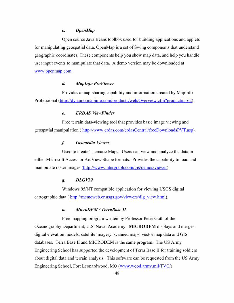
c. OpenMap
Open source Java Beans toolbox used for building applications and applets
for manipulating geospatial data. OpenMap is a set of Swing components that understand
geographic coordinates. These components help you show map data, and help you handle
user input events to manipulate that data. A demo version may be downloaded at
www.openmap.com.
d. MapInfo ProViewer
Provides a map-sharing capability and information created by MapInfo
Professional (http://dynamo.mapinfo.com/products/web/Overview.cfm?productid=62).
e. ERDAS ViewFinder
Free terrain data-viewing tool that provides basic image viewing and
geospatial manipulation ( http://www.erdas.com/erdasCentral/freeDownloadsPVT.asp).
f. Geomedia Viewer
Used to create Thematic Maps. Users can view and analyze the data in
either Microsoft Access or ArcView Shape formats. Provides the capability to load and
manipulate raster images (http://www.intergraph.com/gis/demos/viewer).
g. DLGV32
Windows 95/NT compatible application for viewing USGS digital
cartographic data ( http://mcmcweb.er.usgs.gov/viewers/dlg_view.html).
h. MicroDEM / TerraBase II
Free mapping program written by Professor Peter Guth of the
Oceanography Department, U.S. Naval Academy. MICRODEM displays and merges
digital elevation models, satellite imagery, scanned maps, vector map data and GIS
databases. Terra Base II and MICRODEM is the same program. The US Army
Engineering School has supported the development of Terra Base II for training soldiers
about digital data and terrain analysis. This software can be requested from the US Army
Engineering School, Fort Leonardwood, MO (www.wood.army.mil/TVC/) 48

D. FINAL ANALYSIS
After investigating numerous terrain data tools, the author has come to the
conclusion that there is not one single tool that can solve all data problems (See Figure 4-
1). The choice of the tool depends on its intended use and the users end-state. The
author has identified six tools under $2500 and three that are free of charge to DoD
employees. The most robust capability is achieved through using multiple tools in a
synergistic manner. If resources and time to learn are unconstrained, the best suite of
tools analyzed in this effort are the SOCETSet, SOCETSim and Terratools (plug-in)
family of terrain applications.
Data is also a key element in using any of these applications. If a user does not
have the right data representation in the correct format, the chosen tool may not ever get
the user to their desired end-state.
E. CONCLUSION
In this chapter, the author has explored a variety of mainstream terrain data
manipulation tools available to the government modeling and simulation developer. Each
tool is aimed at filling a particular need in the M&S community. Developers need
different tools to tackle different types of jobs. Different requirements are often driven
by the type of data needed to answer specific questions and are often constrained by the
type of accurate terrain data the developer has available (See Figure 4-1). The list of
applications assessed here is by no means an all-inclusive list of the tools available to
government and civilian developers.
OpenEnviro
49

COST TRAINING KEY FUNTIONALITY DATA SOURCES
SOCETSet $20-30 K 2 Week Course Photogrammetric image exploitation can be output
to OpenFlight and other 3D formats.
Most imagery sources, DTED, USGS
DEM, GeoTIFF, ASCII DTM,
ARCView shape files
SOCETSim $8-10 K 3 Day Course 3D database generation from 2D terrain and
stereo imagery.
DTED, USGS DEM, ASCII DTM,
many stereo imagery sources
Falcon View Free to DOD
Members
One Week
Course
Easy viewing and integration of NIMA products. DTED, CADRG, VMAP, GeoTIFF,
DOQ, many commercial imagery
sources
EdgeViewer Free to DOD
Members
2 Days CBT 2D and 3D visualization tool. Primarily to view
NIMA products.
DTED, CADRG, VPF, ERSI shape
files, ARCView shape files, GeoTIFF,
VRML
TerraTools $2300 (Single) to
$23K (w/GIS &
SOCETSet Plug-ins)
3 Week Course 3D simulation database generation. DTED, DFAD, CADRG, VMAP,
USGS DEM, VPF, ARCView shape
files, AutoCAD, GeoTIFF, XML
Sitebuilder 3D $1,995 1-2 Weeks
Formal & CBT
Builds interactive 3D OpenFlight environment from
2D ARCView products.
DTED, DFAD, ESRI TIN, ESRI GRID,
CAD, GeoTIFF
PVNT Free to DOD
Members
One Week
Formal Training
Builds very high fidelity and accurate terrain
databases for use in analysis.
DTED, many orthophoto and stereo
imagery sources
ARCGIS $1,500 2-4 Weeks of
Formal Training
Builds interactive 3D OpenFlight environment for
terrain visualization and analysis.
DTED, USGS DEM, GeoTIFF, SDTS,
SunRaster
Figure 4-1. Tools Analysis
50

V. APPLIED SUMMARY
Based upon the above exploration of available data formats and representations,
the author has compiled the following guidelines to apply the previous information and
build a basic simulation tool. This step-by-step approach is offered to provide assistance
to those defining and refining terrain space for use in multi-agent system simulation tools.
Initially, developers must define the overall problem set to be solved via the
simulation (See Figure 5-1). The user must then define the terrain space/environment
associated with the problem. This is arguably the hardest step in the development
process. Developers must identify the terrain data representations they wish to use and
the terrain data tools available to manipulate and work with the particular representations.
Unfortunately, the cart often ends up in front of the horse, meaning a developer starts
with a particular terrain data tool, then tries to find an environmental data set that meets
his needs. This is a common approach, but this author does not recommend it. Ideally,
the terrain representation is chosen based on the output desired, then the terrain tool
(ARCVIEW, EdgeViewer etc…) is applied to add-in or pare down the features needed
for the problem set.
The problem in utilizing “the right technique” is that many of the mainstream
terrain manipulation tools are very expensive and time consuming to learn. This is why
the simulation community often takes the “hammer looking for a nail” approach.
Developers often try to force the wrong data and tools into incongruent problem sets.
During problem definition, the developer should begin to consider available
terrain representation data sources. For ground combat agent-based simulation
development, the author recommends DTED as a solid starting point, and notes that it is
the easiest available terrain representation to work with for most developers. Once a
DTED baseline is established, a developer can then use more complex or specialized data
formats such as VPF for refinement.
Based upon the final data-types needed and available, the developer then must
consider available data manipulation tools. It may be necessary to combine multiple
types of data, reduce the data scope, or combine data sets to achieve the desired result.
51

As documented above, data manipulation tools each have positive and negative aspects,
and there is no one “perfect” catchall tool. Due to this fact, the most important factor
becomes the terrain representation and the data formats against which each tool can most
appropriately be applied. In most cases, this problem is addressed by what a developer
knows, not what is the best tool for the job. Learning curves are very steep with many
commercially available tools. The author will now provide a theoretical example
applying this process (See Figure 5-1). This example is completely fictional. Any
similarities to any other systems analysis are completely coincidental.
Step One is to Define the Requirement. In this example the author is building an
Intelligence, Surveillance and Reconnaissance (ISR) analysis tool. The author is
primarily concerned about elevation values (aspect and slope) and vegetation. The author
also needs to build an environment that will provide 2D and 3D visualization inside the
simulation tool. The goal for the project is to understand (analyze) where the dead space
and blind spots are for Airborne and Space surveillance and reconnaissance systems. The
author needs terrain data for Fort Hunter Liggett, California, where much of the actual
system testing will occur. The double boxes in figure 5-1 represent the final products that
will be taken forward into the next step.
Step Two is to Choose the Data Representation that will best suit this
requirement. The author believes that a gridded representation is the best data to use as a
baseline for this project, and has chosen DTED2 as the gridded baseline data
representation. The fidelity of DTED2 is 30-meter terrain postings. The author would
like to use higher fidelity data, but this testing and analysis must be unclassified. If we
use higher fidelity gridded data, the testing environment will likely need to be classified.
The author will first apply the DTED2 data to create a baseline representation. The
author will use raster and stereo imagery data to further refine the terrain set.
52
Step Three is to Choose the Data Manipulation Tool(s) that can work with the
chosen data representations. For this project we need a tool to work with DTED, raster
and stereo imagery. The author chose the SOCETSet/SOCETSim family of tools for this
effort. The SOCET family of tools is an excellent toolkit to create OpenFlight
environments and generate 3D visualization databases from 2D terrain and stereo
imagery. The author will first apply the DTED2 and raster data using SOCETSet. The

author will then apply stereo imagery using SOCETSim. The raster data is very useful
for visualization and complex analysis. The stereo imagery will provide increased
fidelity for a 3D OpenFlight environment. Finally, the author will use SOCETSim to
create a 3D OpenFlight image.
Step Four is to Create the Environment. The author created an OpenFlight 3D
environment of Fort Hunter Liggett in Step Three using the SOCET family. The author
must now define how the autonomous software agents will interact with the environment.
For this application the author will create a two-dimensional array to store the DTED Z
values (terrain postings). DTED data can quickly be converted into a 2D array using a
XML script [Neushul, 2002]. This 2D array will be used to execute agent line of site
calculations for the ISR analysis.
In Step Five, the author will apply this environment and 3D terrain database to the
Multi-Agent System Testbed [Tanner, 1999]. To do this, the author must set up / create
the software agents and place them on the terrain set, either dynamically or deliberately,
give them goals or objectives, and define their interactions with other agents. The author
will set up a placement box where the computer dynamically places the agents in random
starting positions within the defined area. Prior to placing the agents on the terrain, the
developer must create the agents and define their interaction with the terrain and most
importantly with each other. For this ISR analysis requirement, the author will create 50-
100 ground agents in random places in the “play-box”. Their goals are to seek the best
cover and concealment while maintaining maximum visual coverage of the terrain around
them (fields of fire). The author will also create 2 or 3 ISR collection system agents that
will fly the terrain and assess how many ground agents are visible at any given time. The
ISR agents will fly pre-defined search patterns based on specific specifications about how
far and wide an area their sensors can cover. This is a very simple problem set.
Step Six is to Execute the Simulation Runs. Once the simulation database is
created, the developer will execute their simulation runs. The developer will execute as
many simulation runs as necessary to meet the analysis requirement. The author would
expect to collect and analyze the data on 50-100 runs to have a good statistical baseline
for this example.
53

ChooseData
ChooseTool
DTED2 Representation
SOCETSet/SOCETSim
Multi-Agent Testbed
ApplyRaster
CreateAgents
Define Agent InterAction
Fort Hunter Liggett Terrain
ISR Analysis Tool
Apply Imagery
Apply Terrain Set
Convert DTED into2D Array
Place Agentson Terrain
Simulation Database
DTED Baseline
Updated 2D Terrain
Set
OpenFlight Environment
Execute Agent Sim
Runs
Figure 5-1. Data Flow Diagram Example
Once a robust environment has been defined and created, developing a great
simulation is often the easy part. Simulation developers across the globe are very good at
creating complex, dynamic simulation tools. Far too often, developers are weighed down
by the community’s inability to quickly create the right terrain sets in the right format and
the right fidelity. Too often, simulation tools are run on available terrain sets, not on
terrain where the developer envisioned the tool being used. NIMA and other resources
are out there working similar tough terrain problems everyday. Unfortunately, they are
not resourced to do much more than meet real-world requirements.
54
The US Pacific Command is currently developing a notional continent in the
middle of the Pacific Ocean to support multinational simulation exercises in the Pacific
Theater of Operations. The primarily reason for creating this notional continent is to
alleviate the concerns voiced by US allies’ neighbors during multinational training

exercises conducted via simulation. The Exercise Simulation Center – Pacific is in
charge of this effort with strong support from NIMA and the Joint Warfighting Center.
Every agent-based ground combat simulation is a complex, symbiotic system that
should be uniquely based upon the specifications of the developer. The author’s goal has
been to give the reader a grasp of the multitude of issues to be considered while
developing useful combat simulation. Simulation tools have evolved dramatically in the
past decade. The author believes that new simulation techniques, like multi-agent
simulation systems, will grow dramatically in the decades to come. Only high fidelity,
easy-to-create environments will facilitate the evolution of newer techniques to the
forefront of the modeling and simulation of complex joint combat.
55

THIS PAGE INTENTIONALLY LEFT BLANK
56

VI. FUTURE WORK
The author pointed out early in this work that the terrain/environment is only the
first part of creating accurate agent-based ground combat simulation. As the military
moves toward studying how to fight and win battles in urban environments, there will be
an ever-increasing need for higher and higher fidelity simulations. The author envisions
agent-based planning tools will be leveraged to tackle these complex problem sets.
An accurate, physics-based, agent-based simulation could allow trained analysts
to explore the non-tangible types of combat effects. Military modeling and simulations
solutions of the past have accurately modeled the physics, ballistics and line-of-sight of
modern battlefields and weapons systems. There are not, however, standards in place to
model the intangible combat effects of battle, or combat multipliers. How does one
model leadership? How does one model fear? How does one model the psychological
aspects of the battlefield? How do simulation developers address issues such as unit
sustainability, mental health or sleep deprivation? Statistics can help us in this regard by
studying the psychological effects of past battles. Unfortunately, data in these areas is
very scarce or hard to substantiate.
The author believes that the key to incorporating various human factors into
combat simulations, yielding more realistic training and analysis, lies in the opportunities
presented by agent-based systems. Computer scientists in the 1970’s hypothesized that
rule-based artificial intelligence (AI) would be the antecedent to our complex human
behavior representation issues. They were wrong. Scholars and researchers have proven
beyond a reasonable doubt that the complexity of these rule-based models grows too fast
to be useful in our training and analytical simulation tools. They remain, however, very
useful resolving problems of limited scope. Unfortunately these techniques do not scale.
Multi-agent systems are not the solution to all of our military modeling and
simulation problems. These concepts allow a simulation developer to create very
complex systems and systems of systems that are much easier for a simulation developer
to get their head around. These techniques have shown great promise in modeling the
57

complex behavior systems of the contemporary battlefield using relatively simple rule
sets.
58

VII. CONCLUSION
Work in this area will never be complete. The more fidelity given to the
simulation audience, the more fidelity the audience will ask for. Modeling the
environment is a key first step in the development of a mature set of military en route
planning tools.
In this work, the author has tried to lay a solid foundation for further
understanding the digital terrain support available to simulation developers. In chapter 2,
the author presented some background work to provide the reader the requisite
knowledge to understand combat simulation and agent based modeling techniques. The
author proposed a generic formula to create a digital environment to support multi-agent
system simulations. The author discussed previous work on multi-agent systems
conducted by Dr. Andy Ilachinski and related work conducted at the Naval Postgraduate
School.
Chapter III explored the mainstream data representations available to the military
and civilian simulation developer. The author provided a description and conducted an
analysis of many common data representations used in the simulation community.
Additionally, the author discussed some of the organizations involved in the development
of common data formats and standards.
Chapter IV addressed many of the mainstream terrain data manipulation tools
available and provided a brief analysis of each. Many terrain data development
applications are addressed in this work. Each tool has its desirable attributes and specific
utility. Unfortunately, there is not one all-inclusive terrain application to address every
simulation problem set. A good developer must understand the tools available and take
the time to learn the strengths and shortcomings of each application. Data is also a key
ingredient in this process. If a developer does not have the right data set in the right
representation or format, s/he will find great difficulty creating accurate, high fidelity
data sets for agent-based simulations. A quick reference matrix is provided in the final
pages of Chapter IV.
59

Chapter V is an applied summary of Chapters II-IV. The author walks the reader
through the development of a terrain set and multi-agent system tool to analyze Airborne
and Space ISR collection platforms. The author discussed this example from requirement
to data collection and analysis. The author makes some assumptions about this fictional
scenario to walk the reader through some of the choices a developer has to make as they
journey from requirements development to applied autonomous multi-agent simulation
runs.
Chapter VI briefly discusses some advanced concepts and areas of future work.
The Army’s modeling and simulation community has struggled with the development of
reusable terrain data. The Army’s Training, Analytical, and Acquisition simulation
communities have a requirement to develop low, medium and high fidelity terrain sets to
create accurate simulation environments. It is very rare that these terrain sets are shared
between communities. The author will not discuss the details of this disjoint in this work.
He is simply making the point that a tremendous amount of work on terrain sets every
year is completed, but much of this work is never captured or shared with others who
might leverage it.
The author's intent is not to throw stones from inside one’s own glass house, but
to raise awareness about a simulation issue that currently lacks an adequate solution.
Many such issues must be addressed, and good solutions approached, before our current
simulation models mature, evolve, and improve to the point that we can claim to have
accurately modeled the contemporary environment and battlefields of the future.
60

LIST OF REFERENCES
Bailey, Christopher. “PFPS 3.2.” [http://www.falconview.org/]. February 2002. BBN Technologies. “OpenMap™ Open Systems Mapping Technology.” [http://openmap.bbn.com/]. November 2002. Department of Defense, Mandatory Procedures for Major Defense Acquisition Programs and Major Automated Information Systems (DoD 5000.2-R), Washington, DC: U.S. Government Printing Office, 1996. Environmental Systems Research Institute. “ArcView 8.x.” [http://www.esri.com/software/arcgis/arcview/index.html]. October 2002.
Fatale, Louis. “Impact of Digital Terrain Elevation Data (DTED) Resolution on Army Applications: Simulation vs. Reality.” [http://wwwsgi.ursus.maine.edu/gisweb/spatdb/acsm/ac94100.html]. 1994. Federation of American Scientists. “Digital Terrain Elevation Data (DTED).” [http://www.fas.org/irp/program/core/dted.htm]. January 2000. Ferber, J., Multi-Agent Systems: An Introduction to Distributed Artificial Intelligence, London: Addison-Wesley, 1999. Gortler, Steven J. “The 2D Image Domain.” [http://www.eecs.harvard.edu/graphics/chapters/img.pdf]. September 2002.
Headquarters, Department of the Army, Infantry-Based Opposing Force (Field Manual 100-63), Washington, DC: U.S. Government Printing Office, 1996. Holland, J. H., Hidden Order: How Adaptation Builds Complexity, Reading, MA: Addison-Wesley, 1995. Ilachinski, A., Center for Naval Analyses, ISAAC Irreducible Semi-Autonomous Adaptive Combat: An Artificial-Life Approach to Land Warfare, http://www.cna.org/isaac/, 24 July 00. Ilachinski, Andy. “EINSTein: Enhanced ISAAC (Irreducible Semi-Autonomous Adaptive Combat) Neural Simulation Tool.” [http://www.cna.org/isaac/einstein_splash.htm]. February 2000. Ilachinski, A., Irreducible Semi-Autonomous Adaptive Combat (ISAAC): An Artificial-Life Approach to Land Warfare (U), (Center for Naval Analyses Research Memorandum CRM 97-61.10), Alexandria, VA: Center for Naval Analyses, 1997.
61

Mentor Software, Inc. “Geographic Information System (GIS) Tips – Archives.” [http://www.mentorsoftwareinc.com/cc/gistips/TIPSarch.HTM]. June 2002. MultiGen-Paradigm. “SiteBuilder 3D.” [http://www.multigen.com/products/3d_gis/sitebuilder/index.shtml]. 2002. National Imagery and Mapping Agency. “Autometric Viewer: NIMA Purchases Edgeviewer® Software for its Customers.” [http://www.nima.mil/edge_viewer/Edge_Viewer.htm]. February 2002. National Imagery and Mapping Agency. “Military Specification: Compressed ARC Digitized Raster Graphics (CADRG).” [http://164.214.2.59/publications/specs/printed/CADRG/cadrg.html]. February 1996. National Imagery and Mapping Agency. “NIMAMUSE 2.1.” [http://www.nima.mil/geospatial/SW_TOOLS/NIMAMUSE/]. February 2002. National Imagery and Mapping Agency. “Vector Product Format Overview.” [http://www.nima.mil/vpfproto/]. April 2002. Neushul, J., Worldwide Terrain Server, Master’s Thesis, Naval Postgraduate School, Monterey, CA, 2003. Northrop Grumman. “Joint Mapping Toolkit.” [http://www.jmtk.org/]. September 2002. Oregon Department of Forestry Geographic Information Systems. “List of Common GIS Related Acronyms.” [http://www.odf.state.or.us/DIVISIONS/administrative_services/services/gis/acronyms.html]. September 2001. Resnick, M., Turtles, Termites, and Traffic Jams: Explorations in Massively Parallel Microworlds, Cambridge, MA: MIT Press, 1997. SEDRIS™. “The Source for Environmental Representation and Interchange.” [http://www.sedris.org/]. December 2002. Stine, J., Representing Tactical Land Navigation Expertise, Master’s Thesis, Naval Postgraduate School, Monterey, CA, 2000. Tanner, M., Attrition Algorithms Versus Agent-Driven Simulation Models: Richer Simulations Through a Joint paradigm, Interservice/Industry Training, Education and Simulation Conference (I/ITSEC), Orlando, FL, 1999. Tenet Defence. “MapLink Pro Studio – Data Formats.” [http://www.tenetdefence.com/product/maplink/data.htm]. January 2002.
62
TerraSim. “TerraSim Sample Visualizations.” [http://www.terrasim.com/] Texas Natural Resources Information System. “GIS Tools: Map Viewers and Free GIS.” [http://www.tnris.state.tx.us/gistools/mapviewers.htm]. October 2002. U.S. Army Model and Simulation Office. “Environmental Database Integrated Product Team (EDB IPT) Documents.” [http://www.amso.army.mil/terrain/library/documents.htm]. July 2002. U.S. Army Training and Doctrine Command Analysis Center (TRAC), JANUS version 7.06D, [Computer Software], White Sands Missile Range, NM, 1999. United States Geographic Society. “National Mapping Program Standards.” [http://mapping.usgs.gov/standards/]. March 2000. United States Geological Survey. “Geographical Data Download.” [http://edc.usgs.gov/geodata/]. August 2002. United States Geological Survey. “Global 30-Arc-Second Elevation Data Set.” [http://edcwww.cr.usgs.gov/Webglis/glisbin/guide.pl/glis/hyper/guide/gtopo_30]. May 1997. United States Naval Academy, GEODUC Book. “Raster Products.” [http://www.usna.edu/Users/oceano/pguth/website/so432web/e-text/GEODUC_book/Raster%20Products_Ch_6.doc]. November 2001.
63

THIS PAGE INTENTIONALLY LEFT BLANK
64

INITIAL DISTRIBUTION LIST
1. Defense Technical Information Center Ft. Belvoir, Virginia 2. Dudley Knox Library Naval Postgraduate School Monterey, California 3. Dr. Wolfgang Baer Computer Science Department Naval Postgraduate School Monterey, California 4. Curtis Blais Institute for Joint Warfare Analysis Naval Postgraduate School Monterey, California 5. Don Brutzman MOVES Academic Group Naval Postgraduate School Monterey, California
6. Dr. Rudolph P. Darken MOVES Academic Group Naval Postgraduate School Monterey, California
7. MAJ Theodore Dugone Army Modeling and Simulation Office Washington, DC
8. Jack Jackson TRADOC Analysis Center - Monterey Naval Postgraduate School Monterey, California
9. MAJ David W. Laflam Sanbornton, New Hampshire
10. MAJ James D. Neushul Naval Postgraduate School Monterey, California
65

11. MAJ Mark B. Tanner Honolulu, Hawaii
12. Dr. Michael Zyda MOVES Academic Group Naval Postgraduate School Monterey, California
66