CREATING COLOUR The Chemistry of Dyes

Alex Thow

1

Section 1 Introduction

To truly understand the chemistry of dyes we first must consider their colour. Colour has fascinated

humans for thousands of years, from Aristotle believing it was sent from heaven, to Newton separating

light into its colours with a prism. Our curiosity with colour comes from a young age, asking our parents

why the grass is green and the sky blue.

To start this exploration of colour we will look at some basic quantum mechanics to study the behaviour

of light and particles. These ideas can be applied to give an accurate picture of how electrons behave in

atoms and molecules. From this, a description of bonding and delocalisation in organic molecules can

be built up and used to explain how certain molecules can absorb visible light, giving them colour.

The focus of the text will then shift to a more general look at dyes. A glance over the importance of

dyes in human history and their development will be covered before moving into the organic

composition of dyes. We will then look at the structure of some materials and how they can be dyed

and bleached. To finish off our discussions we will consider some specific examples that display how

an understanding of the chemistry of dyes can explain different physical and biological phenomena.

Section 2 Quantum Mechanics

2.1 A Brief History

2.1.1 Blackbody Radiation

In 1900, Max Planck began a scientific revolution. At the time there was a problem, known as the

ultraviolet catastrophe, with something called blackbody radiation. This is the radiation of

electromagnetic waves from an object that absorbs and emits all frequencies of light. A law can be

derived from classical physics, Rayleigh-Jeans’ law, that links the intensity, 𝐵, of radiation to the

frequency, 𝜈.

𝐵(𝜈) =2𝜈2𝑘𝑏𝑇

𝑐2

In this equation, 𝑘𝑏 is the Boltzmann constant, 𝑐 the speed of light in a vacuum and 𝑇 the temperature

of the black body. This law worked for low frequencies but as the frequency increased, it diverged from

the observed spectrum. What Planck did was to assume that the emissions of radiation did not take a

continuous range of energies but had discrete energies proportional to integer multiples of their

frequency.

𝐸 ∝ 𝑛𝜈, 𝑛 = 1, 2, 3 …

He called the constant of proportionality Planck’s constant, ℎ, and used his assumption to create a new

law for blackbody radiation, Planck’s law.

𝐵(𝜈) =2ℎ𝜈3

𝑐2 (𝑒ℎ𝜈

𝑘𝑏𝑇 − 1)

2

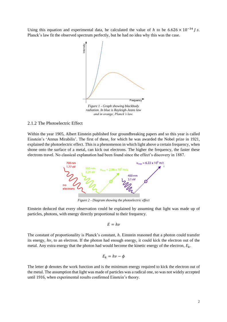
Using this equation and experimental data, he calculated the value of ℎ to be 6.626 × 10−34 𝐽 𝑠.

Planck’s law fit the observed spectrum perfectly, but he had no idea why this was the case.

2.1.2 The Photoelectric Effect

Within the year 1905, Albert Einstein published four groundbreaking papers and so this year is called

Einstein’s ‘Annus Mirabilis’. The first of these, for which he was awarded the Nobel prize in 1921,

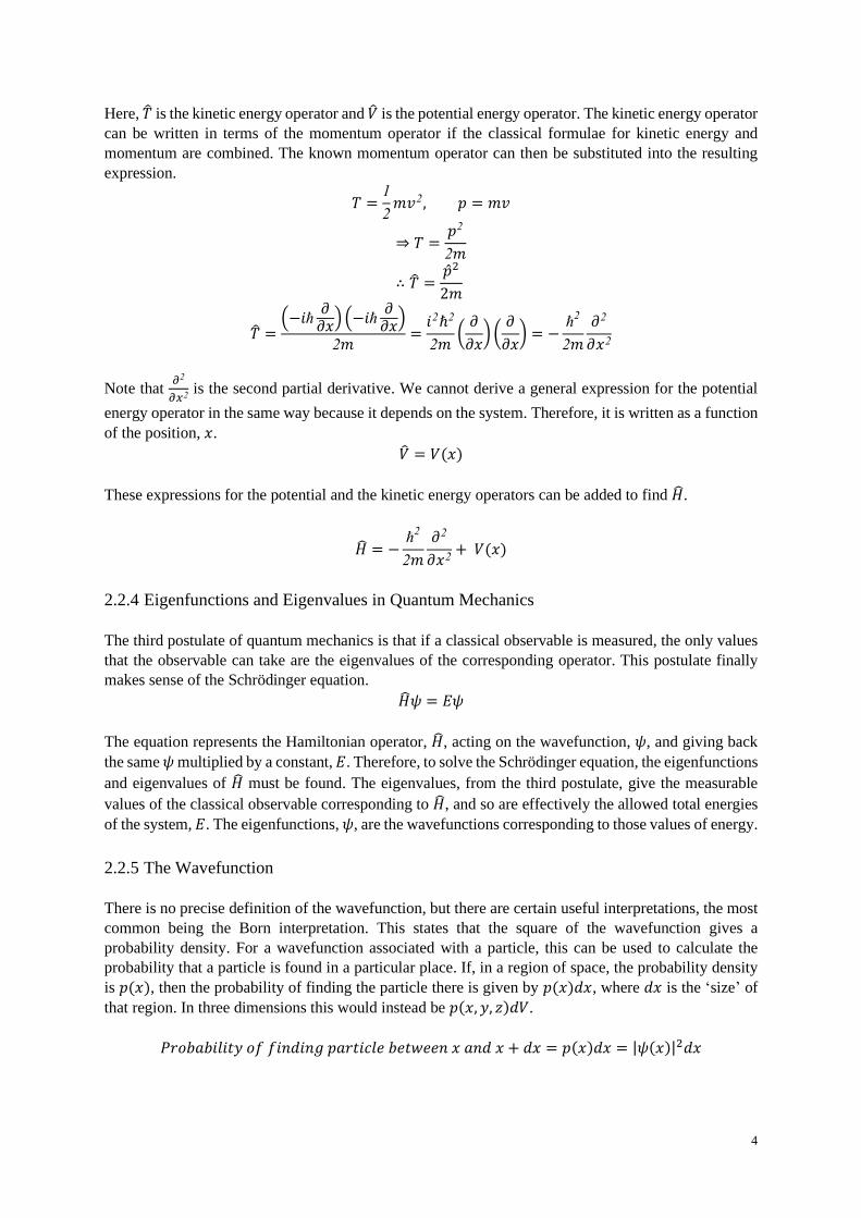
explained the photoelectric effect. This is a phenomenon in which light above a certain frequency, when

shone onto the surface of a metal, can kick out electrons. The higher the frequency, the faster these

electrons travel. No classical explanation had been found since the effect’s discovery in 1887.

Einstein deduced that every observation could be explained by assuming that light was made up of

particles, photons, with energy directly proportional to their frequency.

𝐸 = ℎ𝜈

The constant of proportionality is Planck’s constant, ℎ. Einstein reasoned that a photon could transfer

its energy, ℎ𝜈, to an electron. If the photon had enough energy, it could kick the electron out of the

metal. Any extra energy that the photon had would become the kinetic energy of the electron, 𝐸𝑘.

𝐸𝑘 = ℎ𝜈 − 𝜙

The letter 𝜙 denotes the work function and is the minimum energy required to kick the electron out of

the metal. The assumption that light was made of particles was a radical one, so was not widely accepted

until 1916, when experimental results confirmed Einstein’s theory.

Figure 2 - Diagram showing the photoelectric effect

Figure 1 - Graph showing blackbody

radiation. In blue is Rayleigh-Jeans law

and in orange, Planck’s law.

3

2.2 The Schrödinger Equation

2.2.1 An Introduction

Over the years, quantum theory developed as more rigorous mathematical descriptions were formulated.

Perhaps the most well-known is the Schrödinger equation, which describes something called the

wavefunction of a system, denoted by the Greek letter, 𝜓. The first postulate of quantum mechanics is

that the state of a quantum system is completely specified by the wavefunction. A classical parallel

would be a set containing the positions and momenta of all the particles in a system. Schrödinger’s

equation does have time-dependence, but for the systems we will be covering, a time-independent

equation can be used.

�̂�𝜓 = 𝐸𝜓

2.2.2 Operators, Eigenfunctions and Eigenvalues

The first term of the time-independent Schrödinger equation is �̂�. The hat symbolises that this is an

operator, which is a mathematical object that turns a function into another function. They can take a

wide variety of forms. For example, the operator �̂� = 𝑥 simply multiplies the original function by 𝑥,

whereas the operator �̂� =𝑑

𝑑𝑥 differentiates it with respect to 𝑥.

�̂� sin(𝑘𝑥) = 𝑥 × sin(𝑘𝑥) = 𝑥 sin(𝑘𝑥)

�̂� sin(𝑘𝑥) =𝑑

𝑑𝑥sin(𝑘𝑥) = 𝑘 cos(𝑘𝑥)

For a given operator, �̂�, if a function, 𝑓(𝑥), gives back the same function multiplied by a constant, 𝜆,

that function is called an eigenfunction of �̂� and 𝜆 is the corresponding eigenvalue.

�̂�𝑓(𝑥) = 𝜆𝑓(𝑥)

2.2.3 Operators in Quantum Mechanics

The second postulate of quantum mechanics is that for every classical observable, there is a linear,

Hermitian operator in quantum mechanics. We will not discuss here what it means for the operator to

linear or Hermitian, but all the operators we will see obey both criteria. An example of the second

postulate is that, corresponding to the classical observable of linear momentum along the 𝑥-axis, there

is a quantum mechanical operator, �̂�𝑥.

�̂�𝑥 = −𝑖ℏ𝜕

𝜕𝑥

Note that 𝑖 = √−1, ℏ =ℎ

2𝜋 (the reduced Planck’s constant) and

𝜕

𝜕𝑥 is the partial derivative with respect

to 𝑥, meaning that any other variable is treated as a constant. A discussion of the origins of this operator

is too in-depth for this text, but it can be taken as an axiom.

The operator in the Schrödinger equation, �̂�, is the Hamiltonian operator. It is the operator

corresponding classically to the total energy of a system. From classical mechanics, the total energy is

the sum of the kinetic energy and potential energy.

�̂� = �̂� + �̂�

4

Here, �̂� is the kinetic energy operator and �̂� is the potential energy operator. The kinetic energy operator

can be written in terms of the momentum operator if the classical formulae for kinetic energy and

momentum are combined. The known momentum operator can then be substituted into the resulting

expression.

𝑇 =1

2𝑚𝑣2, 𝑝 = 𝑚𝑣

⇒ 𝑇 =𝑝2

2𝑚

∴ �̂� =�̂�2

2𝑚

�̂� =(−𝑖ℏ

𝜕𝜕𝑥

) (−𝑖ℏ𝜕

𝜕𝑥)

2𝑚=

𝑖2ℏ2

2𝑚(

𝜕

𝜕𝑥) (

𝜕

𝜕𝑥) = −

ℏ2

2𝑚

𝜕2

𝜕𝑥2

Note that 𝜕2

𝜕𝑥2 is the second partial derivative. We cannot derive a general expression for the potential

energy operator in the same way because it depends on the system. Therefore, it is written as a function

of the position, 𝑥.

�̂� = 𝑉(𝑥)

These expressions for the potential and the kinetic energy operators can be added to find �̂�.

�̂� = −ℏ

2

2𝑚

𝜕2

𝜕𝑥2+ 𝑉(𝑥)

2.2.4 Eigenfunctions and Eigenvalues in Quantum Mechanics

The third postulate of quantum mechanics is that if a classical observable is measured, the only values

that the observable can take are the eigenvalues of the corresponding operator. This postulate finally

makes sense of the Schrödinger equation.

�̂�𝜓 = 𝐸𝜓

The equation represents the Hamiltonian operator, �̂�, acting on the wavefunction, 𝜓, and giving back

the same 𝜓 multiplied by a constant, 𝐸. Therefore, to solve the Schrödinger equation, the eigenfunctions

and eigenvalues of �̂� must be found. The eigenvalues, from the third postulate, give the measurable

values of the classical observable corresponding to �̂�, and so are effectively the allowed total energies

of the system, 𝐸. The eigenfunctions, 𝜓, are the wavefunctions corresponding to those values of energy.

2.2.5 The Wavefunction

There is no precise definition of the wavefunction, but there are certain useful interpretations, the most

common being the Born interpretation. This states that the square of the wavefunction gives a

probability density. For a wavefunction associated with a particle, this can be used to calculate the

probability that a particle is found in a particular place. If, in a region of space, the probability density

is 𝑝(𝑥), then the probability of finding the particle there is given by 𝑝(𝑥)𝑑𝑥, where 𝑑𝑥 is the ‘size’ of

that region. In three dimensions this would instead be 𝑝(𝑥, 𝑦, 𝑧)𝑑𝑉.

𝑃𝑟𝑜𝑏𝑎𝑏𝑖𝑙𝑖𝑡𝑦 𝑜𝑓 𝑓𝑖𝑛𝑑𝑖𝑛𝑔 𝑝𝑎𝑟𝑡𝑖𝑐𝑙𝑒 𝑏𝑒𝑡𝑤𝑒𝑒𝑛 𝑥 𝑎𝑛𝑑 𝑥 + 𝑑𝑥 = 𝑝(𝑥)𝑑𝑥 = |𝜓(𝑥)|2𝑑𝑥

5

The total probability of finding the particle anywhere in space is 1, so the sum of the probabilities at

every point in space must equal 1. This is represented mathematically as an integral.

∫ |𝜓(𝑥)|2𝑑𝑥∞

−∞

= 1

A wavefunction that obeys this is said to be normalised, and any wavefunction can be normalised by

multiplying it by some normalisation constant, 𝑁.

∫ 𝑁2|𝜓(𝑥)|2𝑑𝑥∞

−∞

= 1

The Born interpretation imposes some restrictions on the wavefunction:

• The wavefunction must be single-valued because it does not make sense for a particle to have

two different probabilities of being somewhere.

• The wavefunction must be continuous because a break in the wavefunction would lead to a

particle effectively having an undefined probability of being somewhere.

• The wavefunction must be able to be normalised, so must have a finite integral over all space.

Figure 3 - A multi-valued

function. This could not be a

wavefunction.

Figure 4 - A discontinuous

function. This could not be a

wavefunction.

Figure 5 - A function with an

infinite integral. This could not be

a wavefunction.

6

2.2.6 Solving the Schrödinger Equation

The Schrödinger equation can be solved for several systems, including the harmonic oscillator and rigid

rotor. The system we are going to solve it for is called ‘particle in a box’ which consists of a particle

travelling in one dimension between 𝑥 = 0 and 𝑥 = 𝐿. In this region, the potential energy is zero and

outside this region, the potential energy is infinite. This means that the particle cannot leave this region

so perhaps a more suitable name would be ‘particle in an endless hell from which it can never escape’.

As the particle always experiences zero potential energy, the Hamiltonian operator is equal to the kinetic

energy operator.

�̂� = −ℏ2

2𝑚

𝜕2

𝜕𝑥2

Using this, the Schrödinger equation for the system can be written.

−ℏ2

2𝑚

𝜕2

𝜕𝑥2𝜓(𝑥) = 𝐸𝜓(𝑥)

We are looking for a function whose second derivative is itself multiplied by a constant. Luckily, this

has been solved many times before, so we can take a very well-informed guess at the solution.

𝜓(𝑥) = 𝐴 cos(𝑘𝑥) + 𝐵 sin(𝑘𝑥)

The constants 𝐴, 𝐵, and 𝑘 are to be determined. We can now differentiate this function twice.

𝜕

𝜕𝑥(𝐴 cos(𝑘𝑥) + 𝐵 sin(𝑘𝑥)) = −𝑘𝐴 sin(𝑘𝑥) + 𝑘𝐵 cos(𝑘𝑥)

𝜕2

𝜕𝑥2(𝐴 cos(𝑘𝑥) + 𝐵 sin(𝑘𝑥)) =

𝜕

𝜕𝑥(−𝑘𝐴 sin(𝑘𝑥) + 𝑘𝐵 cos(𝑘𝑥)) = −𝑘2𝐴 cos(𝑘𝑥) − 𝑘2𝐵 sin(𝑘𝑥)

∴𝜕2

𝜕𝑥2𝜓(𝑥) = −𝑘2𝜓(𝑥)

This can now be substituted into the Schrödinger equation.

−ℏ2

2𝑚(−𝑘2𝜓(𝑥)) = 𝐸𝜓(𝑥) ⇒

ℏ2𝑘2

2𝑚𝜓(𝑥) = 𝐸𝜓(𝑥) ⇒ 𝐸 =

ℏ2𝑘2

2𝑚

We have derived an expression for the allowed energy levels, which depends on the constant, 𝑘.

Applying boundary conditions, outside the interval [0, 𝐿] there is no probability of finding the particle,

so the wavefunction must be zero at 𝑥 = 0 and 𝑥 = 𝐿.

𝜓(0) = 0 ⇒ 𝐴 cos(0) + 𝐵 sin(0) = 0 ⇒ 𝐴 = 0

𝜓(𝐿) = 0 ⇒ 𝐵 sin(𝑘𝐿) = 0

The constant 𝐵 cannot be zero or the wavefunction would be zero everywhere so sin(𝑘𝐿) must equal

zero. For sin 𝑥 to equal zero, 𝑥 must be an integer multiple of 𝜋.

𝑘𝐿 = 𝑛𝜋 ⇒ 𝑘 =𝑛𝜋

𝐿, 𝑛 = 0, ±1, ±2, ±3, ±4 …

7

This expression for 𝑘 can be inserted into the expressions for the wavefunction and the allowed energy

levels.

𝜓𝑛(𝑥) = 𝐵 sin (𝑛𝜋𝑥

𝐿)

𝐸𝑛 =ℏ2𝑛2𝜋2

2𝑚𝐿2

If 𝑛 = 0, then the wavefunction is simply is zero everywhere so this value is disallowed. If 𝑛 is negative,

the wavefunctions are the positive wavefunctions multiplied by −1. The square of the wavefunction is,

therefore, the same and so these values can also be ignored.

Our final solution to the Schrödinger equation can now be written.

𝜓𝑛(𝑥) = 𝐵 sin (𝑛𝜋𝑥

𝐿) , 𝐸𝑛 =

ℏ2𝑛2𝜋2

2𝑚𝐿2, 𝑛 = 1, 2, 3 …

There is still an undetermined constant, 𝐵, which can be worked out by normalising the wavefunction.

This process will not be covered here as the important result is the allowed energy levels, but the result

is that 𝐵 = √2

𝐿.

Section 3 Atomic and Molecular Orbitals

3.1 A History of Atomic Structure

3.1.1 The Discovery of The Electron

In the late 19th century, there was great interest in cathode rays, which were created when a large

potential difference was applied across a vacuum tube. In 1897, J. J. Thompson directed a stream of

these rays between two charged plates and they deflected towards the positively charged plate. He

concluded that the rays were made of negatively charged particles, electrons. From the magnitude of

the deflection of the rays in electric and in magnetic fields, Thompson calculated the mass of the

electron as only 1

1836 the mass of a proton.

Thompson then suggested a model for the atom called the plum pudding model. This was based on the

knowledge that atoms contained electrons but must also contain positive charge for the overall atom to

be neutral. It consists of electrons distributed within a positively charged medium.

Figure 6 - The plum pudding model of the atom.

8

3.1.2 The Discovery of the Nucleus

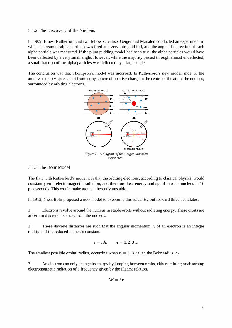
In 1909, Ernest Rutherford and two fellow scientists Geiger and Marsden conducted an experiment in

which a stream of alpha particles was fired at a very thin gold foil, and the angle of deflection of each

alpha particle was measured. If the plum pudding model had been true, the alpha particles would have

been deflected by a very small angle. However, while the majority passed through almost undeflected,

a small fraction of the alpha particles was deflected by a large angle.

The conclusion was that Thompson’s model was incorrect. In Rutherford’s new model, most of the

atom was empty space apart from a tiny sphere of positive charge in the centre of the atom, the nucleus,

surrounded by orbiting electrons.

3.1.3 The Bohr Model

The flaw with Rutherford’s model was that the orbiting electrons, according to classical physics, would

constantly emit electromagnetic radiation, and therefore lose energy and spiral into the nucleus in 16

picoseconds. This would make atoms inherently unstable.

In 1913, Niels Bohr proposed a new model to overcome this issue. He put forward three postulates:

1. Electrons revolve around the nucleus in stable orbits without radiating energy. These orbits are

at certain discrete distances from the nucleus.

2. These discrete distances are such that the angular momentum, 𝑙, of an electron is an integer

multiple of the reduced Planck’s constant.

𝑙 = 𝑛ℏ, 𝑛 = 1, 2, 3 …

The smallest possible orbital radius, occurring when 𝑛 = 1, is called the Bohr radius, 𝑎0.

3. An electron can only change its energy by jumping between orbits, either emitting or absorbing

electromagnetic radiation of a frequency given by the Planck relation.

Δ𝐸 = ℎ𝜈

Figure 7 - A diagram of the Geiger-Marsden

experiment.

9

This model of the atom quantises the energy levels of the electrons and can accurately predict the

frequency of the lines in the emission spectrum of hydrogen. But just like the other models, it eventually

was replaced by the modern theory of atomic orbitals.

3.2 Atomic Orbitals

3.2.1 An Introduction to Orbitals

In Bohr’s model, we know the electron’s exact distance from the nucleus and its momentum. This

violates Werner Heisenberg’s uncertainty principle. We will not derive this, but it means we can never

know both the position and momentum of any particle with complete accuracy. The product of their

uncertainties must be greater than or equal to half of the reduced Planck’s constant.

𝜎𝑥𝜎𝑝 ≥ℏ

2

To solve this issue, the electrons must be described by wavefunctions. This means only knowing the

probability of an electron being somewhere, not exactly where it is, no longer violating the uncertainty

principle. These wavefunctions are atomic orbitals.

3.2.2 A Mathematical Description of Orbitals

The Schrödinger equation can be used to find mathematical expressions for the atomic orbitals.

Unfortunately, it can only be solved exactly for single-electron systems as with multiple electrons there

are too many interactions to deal with. However, these solutions do provide a good description of atomic

orbitals in general.

For atomic orbitals, it is much easier to use polar coordinates than Cartesian coordinates. Cartesian

coordinates use the variables 𝑥, 𝑦 and 𝑧. Polar coordinates use the distance from the origin 𝑟, and two

angles, 𝜃 and 𝜙.

Figure 8 - Diagram showing an electron

losing energy via emission of a photon.

Figure 9 - Diagram showing polar

coordinates.

10

When the Schrödinger equation is solved for a hydrogen atom, each wavefunction is characterised by

three quantum numbers, similar to how the particle in a box wavefunction was characterised by 𝑛:

1. The principal quantum number, 𝑛, takes values 1, 2, 3 …

2. The angular momentum quantum number, 𝑙, takes values 0, 1, 2 … , 𝑛 − 1

3. The magnetic quantum number, 𝑚𝑙, takes values −𝑙 … , −1, 0, +1 … , +𝑙.

The principal quantum number determines the shell the electron is in and can completely determine the

energy of a hydrogen orbital.

𝐸𝑛 = −𝑍2𝑅𝐻

𝑛2

The nuclear charge, 𝑍, is simply 1 for hydrogen and the Rydberg constant, 𝑅𝐻, has a value of

2.180 × 10−18 𝐽. The energy is negative because a free electron is said to have zero energy and when

bound by a nucleus it has less energy.

The principal and angular momentum quantum numbers determine the subshell an electron is in. For

each value of 𝑙 there is a corresponding letter, 𝑙 = 0 is 𝑠, 𝑙 = 1 is 𝑝, 𝑙 = 2 is 𝑑 and 𝑙 = 3 is 𝑓. The

possible values of 𝑙 mean that in the first shell there is only an 𝑠 subshell, in the second only 𝑠 and 𝑝

subshells and so on.

The principal, angular momentum and magnetic quantum numbers determine the orbital the electron is

in. For the 𝑠 subshells, 𝑚𝑙 can only be 0 so there is one 𝑠 orbital per subshell. For the 𝑝 subshells, 𝑚𝑙

can be −1, 0, or 1, so there are three 𝑝 orbitals per subshell. In the same way, there are five 𝑑 and seven

𝑓 orbitals per subshell. The orbitals are distinguished by a subscript. For example, 2𝑝𝑥 , 2𝑝𝑦 and 2𝑝𝑧 are

the three 𝑝 orbitals in the second shell.

The wavefunctions of hydrogen can be written as the product of a radial part, 𝑅, and an angular part, 𝑌.

𝜓𝑛,𝑙,𝑚𝑙(𝑟, 𝜃, 𝜙) = 𝑅𝑛,𝑙(𝑟) × 𝑌𝑙,𝑚𝑙

(𝜃, 𝜙)

The probability of an electron being found at a certain distance, 𝑟, from the nucleus can be calculated

by multiplying the probability density of a point at that distance from the nucleus, 𝑝(𝑟), by the surface

area of a sphere of that radius.

𝑆𝑢𝑟𝑓𝑎𝑐𝑒 𝑎𝑟𝑒𝑎 𝑜𝑓 𝑠𝑝ℎ𝑒𝑟𝑒 = 4𝜋𝑟2

𝑃𝑟𝑜𝑏𝑎𝑏𝑖𝑙𝑖𝑡𝑦 𝑑𝑒𝑛𝑠𝑖𝑡𝑦 𝑜𝑓 𝑒𝑙𝑒𝑐𝑡𝑟𝑜𝑛 𝑎𝑡 𝑟𝑎𝑑𝑖𝑢𝑠 𝑟 = 4𝜋𝑟2𝑝(𝑟)

From the Bohr interpretation, the probability density, 𝑝(𝑟), is the square of the wavefunction. This

defines the radial distribution function, 𝑃(𝑟), which is effectively a measure of the electron densities at

different radii.

𝑃(𝑟) = 4𝜋𝑟2|𝜓(𝑟)|2

3.2.3 A Closer Look at the 𝑠 Orbitals

The simplest orbital is the 1𝑠 orbital, whose wavefunction we will consider now.

𝜓1𝑠 = 𝑁1𝑠𝑒−

𝑟𝑎0

11

𝑁1𝑠 is a normalisation constant whose value is not important and 𝑎0 is the Bohr radius. The value of the

wavefunction only depends on the distance from the nucleus, so the orbital has spherical symmetry.

The wavefunction has a maximum in the centre of the nucleus and decays exponentially outwards. The

radial distribution function has a maximum at 𝑟 = 𝑎0, so the electron density is highest at this radius.

The issue with depicting orbitals on paper is that there are not enough dimensions. There are several

ways of overcoming this, but each has its flaws. The one we are going to use is created by taking a

cross-section through the orbital and plotting large numbers of dots based on the value of the

wavefunction. The denser the dots, the higher the value of the wavefunction.

The wavefunction of the 2𝑠 orbital is slightly more complex than that of the 1𝑠.

𝜓2𝑠 = 𝑁2𝑠 (2 −𝑟

𝑎0) (𝑒

−𝑟

2𝑎0)

Just like the 1𝑠, this orbital is spherically symmetric. To compare the 2𝑠 orbital to the 1𝑠 their radial

distribution functions can be plotted on the same graph.

Figure 10 - Graph of the 1s wavefunction, blue, and radial

distribution function, orange.

Figure 11 - Dot representation

of the 1s orbital.

Figure 12 - Graphs of the radial distribution functions of the 1s, blue, and

2s, orange.

12

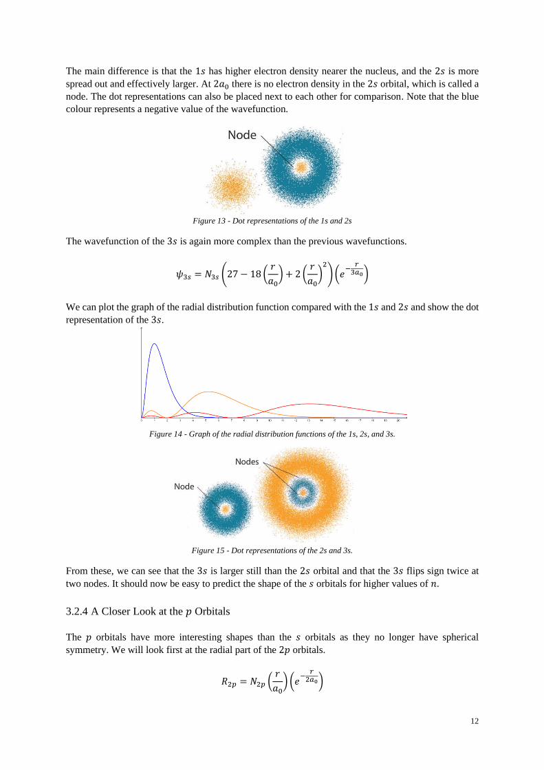
The main difference is that the 1𝑠 has higher electron density nearer the nucleus, and the 2𝑠 is more

spread out and effectively larger. At 2𝑎0 there is no electron density in the 2𝑠 orbital, which is called a

node. The dot representations can also be placed next to each other for comparison. Note that the blue

colour represents a negative value of the wavefunction.

The wavefunction of the 3𝑠 is again more complex than the previous wavefunctions.

𝜓3𝑠 = 𝑁3𝑠 (27 − 18 (𝑟

𝑎0) + 2 (

𝑟

𝑎0)

2

) (𝑒−

𝑟3𝑎0)

We can plot the graph of the radial distribution function compared with the 1𝑠 and 2𝑠 and show the dot

representation of the 3𝑠.

From these, we can see that the 3𝑠 is larger still than the 2𝑠 orbital and that the 3𝑠 flips sign twice at

two nodes. It should now be easy to predict the shape of the 𝑠 orbitals for higher values of 𝑛.

3.2.4 A Closer Look at the 𝑝 Orbitals

The 𝑝 orbitals have more interesting shapes than the 𝑠 orbitals as they no longer have spherical

symmetry. We will look first at the radial part of the 2𝑝 orbitals.

𝑅2𝑝 = 𝑁2𝑝 (𝑟

𝑎0) (𝑒

−𝑟

2𝑎0)

Figure 13 - Dot representations of the 1s and 2s

Figure 14 - Graph of the radial distribution functions of the 1s, 2s, and 3s.

Figure 15 - Dot representations of the 2s and 3s.

13

To understand this, we can plot the radial distribution function of the 2𝑝 orbitals compared with the 1𝑠

and 2𝑠.

It is a similar size to the 2𝑠 orbital, which should not be surprising as it has the same energy. It has no

radial nodes, but it does have another type of node not seen in the radial part. The angular part depends

on the particular 𝑝 orbital.

𝑌𝑝𝑧= cos(𝜃) , 𝑌𝑝𝑥

= sin(𝜃) cos(𝜙) , 𝑌𝑝𝑦= sin(𝜃) sin(𝜙)

Explaining what these mean mathematically can get confusing, so we will simply look at the result

using the dot representation.

Each orbital has a nodal plane, shown in the diagram by a dotted line. Each side of this dotted line the

wavefunction has the opposite sign. It turns out that each orbital has cylindrical symmetry, meaning it

is symmetrical by rotation about a certain axis. The 2𝑝𝑧 lies along the 𝑧-axis and so on. Going into

detail discussing any more orbitals is unnecessary for our future discussions so they will be left here.

3.2.5 Multi-Electron Atoms

For more complex atoms, we are adding electrons and increasing the nuclear charge. It is impossible to

solve the Schrödinger equation analytically for these systems, so approximations and numerical

methods are used to find the wavefunctions.

The way electrons occupy the orbitals is governed by their energy and the Pauli exclusion principle. An

electron in hydrogen will usually occupy the lowest energy orbital, the 1𝑠, but in multi-electron atoms,

the electrons start to occupy different orbitals. This is because the Pauli exclusion principle prevents

two electrons from having identical quantum numbers. There is a quantum number that we have not

Figure 16 - Graph of the radial distribution functions of the 1s, blue, 2s,

orange, and 2p, red.

Figure 17 - Dot

representation of the

2pz.

14

mentioned yet, spin. Electrons can either have a spin of +1

2 (spin-up) or −

1

2 (spin-down). The result is

that at most two electrons can occupy any orbital, as long as they have opposite spin. Therefore,

electrons fill up the orbitals two at a time from lowest energy to highest energy.

The energies of the orbitals change in multi-electron atoms such that those with the same 𝑛 no longer

need have the same energy. We will not go into a detailed discussion as to why this is, but we will show

a graph of the energies of some of the orbitals as you increase the atomic number.

The unit of electron volts, 𝑒𝑉, makes the numbers easier to deal with as 1 𝑒𝑉 = 1.60 × 10−19 𝐽. When

the 1𝑠 orbital is full, the electrons then go into the 2𝑠 as this is actually lower in energy than the 2𝑝.

Then they go into the 2𝑝, then the 3𝑠, and so on. The results can be summarised in an electron

configuration. For fluorine, it would be 1𝑠22𝑠22𝑝5. This shows that there are two electrons in both the

1𝑠 and 2𝑠 subshells, and five in the 2𝑝 subshell.

3.3 Diatomic Molecular Orbitals

3.3.1 The Simple Case – H2+

Due to the presence of only one electron in H2+, it is possible to solve the Schrödinger equation and the

result is a molecular orbital (MO). MOs are filled up by electrons in order of increasing energy, just

like atomic orbitals (AOs). For molecules with multiple electrons, some rules can be used to guess the

form of the MOs and their relative energies, all of which can be derived from quantum mechanics.

One simple approach is called the linear combination of atomic orbitals, LCAO. This takes the algebraic

sum of the AOs at every point in space to construct the MO.

𝑀𝑂 = 𝑐1(𝐴𝑂1) + 𝑐2(𝐴𝑂2)

The constants, 𝑐1 and 𝑐2, are orbital coefficients which can be determined through detailed quantum

mechanical calculations. In the H2+ molecule, it would make sense for the lowest energy MO to be

constructed from a combination of the two 1𝑠 orbitals. It turns out that there are two MOs formed from

the combination of these AOs. For the first, 𝑐1 = 𝑐2 = 1 and for the second, 𝑐1 = 1, 𝑐2 = −1.

𝑀𝑂1 = 𝑁1(1𝑠 𝑜𝑓 𝑓𝑖𝑟𝑠𝑡 𝑎𝑡𝑜𝑚 + 1𝑠 𝑜𝑓 𝑠𝑒𝑐𝑜𝑛𝑑 𝑎𝑡𝑜𝑚)

𝑀𝑂2 = 𝑁2(1𝑠 𝑜𝑓 𝑓𝑖𝑟𝑠𝑡 𝑎𝑡𝑜𝑚 − 1𝑠 𝑜𝑓 𝑠𝑒𝑐𝑜𝑛𝑑 𝑎𝑡𝑜𝑚)

-140

-120

-100

-80

-60

-40

-20

0H H

e

Li Be

B C N O F Ne

Na

Mg

Al

Si P S Cl

Ar

Ener

gy/e

V

1s

2s

2p

3s

3p

Figure 18 - Graph of the energy of orbitals in the first 18 atoms.

15

Again, 𝑁1 and 𝑁2 are normalisation constants. When the atoms are far apart, the MOs will effectively

be identical in shape to the AOs. At shorter distances, MO1 will contain a region between the nuclei

where the AOs are adding together and producing high electron density, called constructive overlap.

For MO2, the AOs are subtracting and producing low electron density, called destructive overlap.

Halfway between the nuclei, there will be a node of zero electron density.

In H2+, the lowest energy MO turns out to be MO1, so the electron occupies this orbital. This creates

high electron density between the nuclei and pulls them towards each other until the attraction balances

the repulsion of the nuclei. This is a chemical bond and so MO1 is described as a bonding orbital. If the

electron were for some reason to be MO2, then the low electron density between the nuclei means that

the repulsive force is strong, and the electron density either side of the nuclei pulls them apart. For this

reason, MO2 is described as an antibonding orbital.

Molecular orbitals can be classified using symmetry. In H2+, the orbitals are symmetric by rotation about

the internuclear axis, and so are called 𝜎 orbitals. The only other type of orbital we will meet is one

where rotation by 180° about the internuclear axis flips the sign of the wavefunction. This is called a 𝜋

orbital. Bonds formed by these orbitals are called 𝜎 and 𝜋 bonds, respectively. Antibonding orbitals are

given an asterisk, for example 𝜎∗.

The energies of MOs can be represented on a MO diagram. The horizontal lines represent orbitals, with

those at the sides being the original AOs, and those in the centre being the MOs. At large separation,

the lines are the same level as the MOs are equivalent to the AOs. As the atoms get closer, the bonding

MO lowers in energy and the antibonding MO increases in energy.

3.3.2 More Complex Cases – H2, He2+, and He2

The MOs can be filled in a similar way to how AOs are filled. Two electrons are placed in each orbital

with opposite spin, starting with the lowest energy orbital. For the simple case of two 1𝑠 orbitals

forming a 𝜎 and a 𝜎∗ orbital, it can be seen that the first two electrons fill the 𝜎 and the next goes into

the 𝜎∗. This can be represented using MO diagrams.

Figure 19 – H2+ molecular orbitals.

Figure 20 - MO diagrams for overlap of 1s orbitals at large

(left) and small (right) separation.

Figure 21 - Molecular orbital diagrams of

H2+ (left), H2 (centre) and He2

+ (right).

16

If we were to add another electron it would go into the 𝜎∗ orbital. It turns out that the 𝜎∗ orbital is

slightly more raised in energy than the 𝜎 is lowered. This would mean that going from two He atoms to

an He2 molecule would lead to a net increase in energy, showing why helium does not form diatomic

molecules.

3.3.3 Rules of Forming Molecular Orbitals

We will not cover how these rules are derived but they are very useful for constructing MOs from AOs.

1. If 𝑛 AOs are combined, 𝑛 MOs are formed.

2. AOs can only combine if they have the correct symmetry.

3. AOs that are closer in energy have a larger interaction when forming MOs.

4. AOs which are closer in energy to an MO contribute more to it.

5. AOs can only interact strongly if their sizes are compatible.

The first of these is quite simple to understand. If we pull apart a molecule, the MOs will steadily

become AOs. Since this must be a continuous process, the number of orbitals cannot change.

To understand the second, we will cover a disallowed interaction. If we try to combine a 2𝑠 and a 2𝑝𝑥

orbital, taking the internuclear axis to be the 𝑧-axis, then one lobe of the 2𝑝𝑥 orbital will constructively

overlap with the 2𝑠 and the other will destructively overlap with it. The overlaps will be equal and

opposite and so the total overlap will be zero, so these AOs do not form an MO. For a 2𝑠 and 2𝑝𝑧, this

is not a problem and so an MO can be formed.

The third rule can be easily explained with MO diagrams.

It can be seen that as the difference in energy between the AOs increases, the MOs become closer in

energy to the original AOs, so the interaction decreases. The fourth rule is self-explanatory and simply

means that the higher energy AO contributes more to the antibonding MO and vice versa.

Figure 22 - Diagram showing the disallowed

overlap between 2s and 2px (left) and allowed

overlap between 2s and 2pz (right).

Figure 23 - MO diagrams showing how AOs

of the same energy (left) combine compared

to AOs of different energies (right).

17

The fifth rule is also a result of the overlap as, if the two orbitals differ greatly in size, then the overlap

will not be effective, and the AOs will not interact strongly.

3.3.4 Combining Different Atomic Orbitals

When 2𝑠 orbitals are combined the result is simple and we end up with another 𝜎 and 𝜎∗ of higher

energy than with a combination of 1𝑠 orbitals. When 2𝑝𝑧 orbitals are combined, as these lie on the

internuclear axis, we get another 𝜎 and 𝜎∗, which are higher in energy still. They are, however, slightly

different from the 𝜎 MOs created from 𝑠 orbitals.

When 2𝑝𝑥 and 2𝑝𝑦 orbitals are combined, the resulting MOs are 𝜋 and 𝜋∗. These do not have cylindrical

symmetry and so look more complex than the 𝜎 orbitals.

With this knowledge, we can draw an MO diagram displaying the bonding between many different

atoms. As an example, we will draw one for the nitrogen molecule. For simplicity, we will assume that

only interactions between identical orbitals can occur, although in reality the 𝑠 and 𝑝 orbitals can

interact.

The 1𝑠 interactions have been ignored as they are much lower in energy. The most important

interactions are those of the 𝑝 orbitals, and the order of energy of their MOs is 𝜎, 𝜋, 𝜋∗, 𝜎∗. The electrons

shown fill four bonding MOs and one antibonding, giving N2 an overall triple bond.

Figure 24 - Diagram showing the bonding (top) and antibonding (bottom) MOs

created from two 2pz orbitals.

Figure 25 - Diagram showing the bonding (top) and antibonding

(bottom) MOs created from two 2px or 2py orbitals.

Figure 26 - MO diagram for the N2 molecule.

18

Section 4 Bonding in Organic Molecules and Colour

4.1 Hybridisation

4.1.1 An Introduction to Hybrid Orbitals

When describing bonding in organic molecules, using the molecular orbitals described in the last section

would be almost impossible. For more than a few atoms there are too many interactions to deal with,

and the molecular orbitals become very difficult to interpret. Hybridisation is a different approach that

helps solve this issue.

Hybridisation is the mixing of AOs to creating hybrid atomic orbitals (HAOs). These HAOs often

combine to form much more simple MOs. For example, with methane, the issue with using the full MO

approach is that the AOs do not point directly towards the four hydrogen atoms. The 2𝑠 points equally

in all directions and the 2𝑝 orbitals point at right-angles, not at the tetrahedral angle of 109.5°. The

hybrid approach allows for four simple HAOs that point directly to each hydrogen, creating simple

MOs.

4.1.2 Different HAOs – 𝑠𝑝3, 𝑠𝑝2, and 𝑠𝑝

In organic molecules, we are usually considering bonding to carbon atoms. If the carbon atom is bonded

to four other atoms, four different HAOs need to be formed just like in methane. The way this is done

is by directly combining the single 2𝑠 orbital with the three 2𝑝 orbitals. The new orbitals are 𝑠𝑝3

hybridised. Each of these are identical and are separated by 109.5°.

The energy of this hybrid orbital is between the energy of the 2𝑠 and 2𝑝 orbitals and turns out to be

similar in energy to the 1𝑠 orbital of a hydrogen atom. We can draw an MO diagram for the combination

of an 𝑠𝑝3 HAO with a hydrogen 1𝑠 AO. There is one electron contributed from each orbital and so both

go into the bonding MO, forming a C-H bond.

Figure 27 - Diagram showing the

HAOs of methane.

Figure 28 - MO diagrams showing the creation of sp3

HAOs (left) and the creation of a C-H bond (right).

19

When a carbon is double bonded to an atom, we must use a different hybridisation. The required HAOs

should be at 120° to each other and in the same plane. This can be done by combining the 2𝑠 orbital

with only two of the 2𝑝 orbitals. This creates three 𝑠𝑝2 hybridised orbitals and a leftover 2𝑝 orbital. In

the case of ethene, C2H4, each carbon has two 𝜎 bonds to hydrogens created by a combination of the

hydrogen 1𝑠 and an 𝑠𝑝2 HAO from the carbon. There is also a 𝜎 bond between the two carbons created

by the head-on overlap of two 𝑠𝑝2 HAOs. Finally, the double bond is a 𝜋 bond formed by the overlap

of the leftover 2𝑝 orbitals.

Finally, when a carbon has a triple bond, it must be 𝑠𝑝 hybridised. This leaves two 2𝑝 orbitals that can

generate two 𝜋 bonds in addition to the 𝜎 bond, creating a triple bond. This can be used to describe the

bonding in ethyne, C2H2.

4.2 Delocalisation and Conjugation

4.2.1 Delocalised Bonding

So far, we have covered localised bonding, meaning that the bonding occurs between two atoms. This

gives an accurate picture in most circumstances, but there are notable exceptions where this fails to

explain certain properties of a molecule, giving rise to delocalised bonding.

One well-known example is benzene, a molecule with the molecular formula C6H6. In 1865, August

Kekulé proposed a structure for benzene.

Figure 29 - Diagram showing the 𝜎 and 𝜋

interactions in ethene.

Figure 30 - Diagrams to show the interactions in

ethyne. One helps show the 𝜎 bond (left) and one

the 𝜋 bonds (right).

Figure 31 - Kekulé

structure of benzene.

20

A double bond is stronger and therefore shorter than a single bond, so we would expect benzene to have

alternating long and short bonds. However, it turns out that each bond length is identical and

approximately halfway between that of a single bond and a double bond. This suggests that each bond

is effectively one and a half bonds. This is because the electrons in the 𝑝 orbitals of benzene are

delocalised over all six carbon atoms equally, and so instead of alternating double and single bonds, a

circle is drawn.

To represent delocalisation, multiple structures can be drawn with a double-headed arrow between

them. This means that the molecule is somewhere between these two forms. The curly arrows here do

not represent a reaction but simply that the electrons are delocalised around the ring.

As benzene chooses to adopt this delocalised form, we can conclude that delocalisation is a stabilising

effect.

4.2.2 Delocalisation in Carbon Chains

Delocalisation is not confined to rings but shows up in many different organic molecules. For example,

trans-hexatriene.

There are two main issues with a localised bonding description of this molecule. One is that the

molecule should rotate freely about the single bonds, but it turns out to be planar. The other is that the

single bonds are shorter than they should be and the double bonds slightly longer.

If we carry over the idea from benzene that the 𝑝 orbitals can delocalise over the whole molecule, then

we can understand why it is planar. If the molecule were not planar, the 𝑝 orbitals would not overlap

effectively. It adopts a planar form to maximise delocalisation and its stabilising effect.

Figure 32 - Delocalised

structure of benzene.

Figure 33 - Diagram showing the delocalisation in

benzene.

Figure 34 - Trans-hexatriene.

Figure 35 - Diagram showing why trans-hexatriene is planar.

21

Conjugation is the presence of alternating double and single bonds and it allows for 𝑝 orbital

delocalisation. Note that if two single bonds separate the double bonds, the 𝑝 orbitals are too far away

to overlap and if there are two double bonds directly next to each other, the 𝑝 orbitals lie perpendicular

to each other and cannot overlap. A clear example of an extended conjugated system is in 𝛽-carotene,

the molecule that gives carrots their orange colour.

4.2.3 Other Examples of Delocalisation

Delocalisation does not just occur over carbon atoms. A good example is in propenal.

There are two double bonds separated by a single bond, so this molecule is conjugated. The presence

of an oxygen changes the energies of the 𝑝 orbitals, but they still overlap. The resultant MO covering

the whole molecule is not symmetric, but there is still delocalisation.

Charge on a molecule can create delocalisation where otherwise it would not be seen. An example is

the allyl anion.

There is only one double bond, but the rightmost carbon is 𝑠𝑝2 hybridised with a leftover 𝑝 orbital, in

which there are two electrons. This 𝑝 orbital can delocalise with the 𝑝 orbitals of the double bond. This

delocalisation makes the anion symmetric.

4.2.4 The Molecular Orbitals of Conjugated Systems

Now we can discuss the form of the MOs that the overlapping 𝑝 orbitals create. To do this we will

consider how the 𝜋 and 𝜋∗ MOs combine. One of the simplest examples is 1,3-butadiene.

Figure 36 – The clear conjugated system in 𝛽-carotene.

Figure 37 - Propenal.

Figure 38 - Allyl

anion.

Figure 39 - Diagram showing how delocalisation makes

the allyl anion symmetric.

Figure 40 - 1,3-butadiene.

22

We are combining two 𝜋 and two 𝜋∗ localised MOs, so we will create a total of four new delocalised

MOs. The lowest energy combination will be when the two 𝜋 MOs combine in phase (constructively),

so there are no nodes. The next highest will be when the two 𝜋 MOs combine out of phase

(destructively), creating a node through the central bond. Then we combine the two 𝜋∗ MOs in phase,

creating two nodes. The highest energy orbital will be when the two 𝜋∗ MOs combine out of phase.

This can be represented on an MO diagram. Notation is to label the new MOs 𝜓1, 𝜓2, 𝜓3, and 𝜓4 in

order of increasing energy.

The diagram has been filled with four electrons, two from each 𝜋 orbital, and the total effect is a slight

lowering of energy. The highest energy orbital with electrons in it is called the HOMO (highest energy

occupied molecular orbital), and the lowest energy orbital without electrons in it is called the LUMO

(lowest energy unoccupied molecular orbital).

4.3 Colour of Conjugated Systems

4.3.1 Modelling Conjugated Systems with Particle in a Box

We can now explain the absorbance of visible light by conjugated systems. When light is shone on a

molecule with a conjugated system, an electron can absorb a photon of the right frequency to jump from

the HOMO of that conjugated system to the LUMO. The frequency of the light depends on the energy

difference between the HOMO and LUMO via the Planck relation ∆𝐸 = ℎ𝜈.

Figure 41 - Diagrams depicting how the 𝜋 and 𝜋∗

MOs combine.

Figure 42 - MO diagram showing the energies of the

MOs in butadiene.

23

To energies of the HOMO and LUMO can be estimated using particle in a box. An electron moving

through a conjugated system can be thought of as a particle moving from one end of the conjugated

system to the other as the electron is effectively trapped within the molecule. For simplicity, we will

deal only with conjugated systems in simple carbon chains.

4.3.2 Calculating the Colour of Molecules

We have already derived the energy levels for particle in a box.

𝐸𝑛 =ℏ2𝑛2𝜋2

2𝑚𝐿2

We can turn this into a formula depending on the number of double bonds in a straight-chain conjugated

system, 𝑘. The length of the system, 𝐿, can be approximated by taking the average bond length, 𝑅,

which is approximately the mean of the C=C and C-C average bond lengths, and multiplying it by the

total number of bonds in the chain, which is 2𝑘 − 1.

𝐿 ≈ (2𝑘 − 1)𝑅

To work out the difference in energy between the HOMO and the LUMO, we must write 𝑛, the energy

level, in terms of 𝑘. Each double bond contributes two electrons to the conjugated system, but there are

two electrons per energy level and so for the HOMO, 𝑛 = 𝑘. The energy level of the LUMO is therefore

𝑛 = 𝑘 + 1.

∆𝐸 = 𝐸𝐿𝑈𝑀𝑂 − 𝐸𝐻𝑂𝑀𝑂 =ℏ2(𝑘 + 1)2𝜋2

2𝑚𝐿2−

ℏ2𝑘2𝜋2

2𝑚𝐿2=

ℏ2𝜋2

2𝑚𝐿2((𝑘 + 1)2 − 𝑘2) =

ℏ2𝜋2

2𝑚𝐿2(2𝑘 + 1)

Into this, we can substitute the Planck relation, ∆𝐸 = ℎ𝜈 =ℎ𝑐

𝜆.

∆𝐸 =ℎ𝑐

𝜆=

ℏ2𝜋2

2𝑚𝐿2(2𝑘 + 1) ⟹ 𝜆 =

2𝑚𝐿2ℎ𝑐

ℏ2𝜋2(2𝑘 + 1) =

8𝑚𝑐

ℎ(

𝐿2

2𝑘 + 1)

∴ 𝜆 =8𝑚𝑐

ℎ(

𝑅2(2𝑘 − 1)2

2𝑘 + 1)

In this equation, 𝑚, the mass of an electron, ℎ, 𝑐, and 𝑅 are all constants. Given the number of double

bonds, we have an equation that gives us the absorbed wavelength of light. The colour that the molecule

appears will be the complementary colour to the absorbed colour.

Figure 43 - A colour wheel can be used to

easily work the colour of a molecule given

the wavelength it absorbs.

24

Let us calculate values for the absorbed wavelength for 𝑘 = 1 − 5.

Past this, the calculated wavelength diverges from the actual value as this method is just an

approximation. However, we are shown the very important point that a molecule must have a conjugated

system of a reasonable length, at least five or six double bonds, to absorb in the visible spectrum. These

extended conjugated systems turn out to be what give dyes their colour.

Section 5 Terminology and History of Dyes

5.1 Some Simple Terminology

To avoid confusion in our later discussions of dyes, there are a few terms that should be defined.

• Dye – A water-soluble organic substance that is coloured and can impart colour to an object,

e.g., betanin (found in beetroot).

• Pigment – A water-insoluble, coloured, inorganic substance, e.g., hematite (Fe2O3).

• Fastness – The resistance of a dye to being removed from a material by washing or by exposure

to light or heat.

5.2 History of Dyes

5.2.1 Ancient History

Dyes have a very long history. The first appearance of dyes is debated but prehistoric rock paintings,

done using pigments, dating back to thousands of years BC are believed to depict coloured garments.

One of the oldest dyes is indigo, used in denim. The oldest example of an indigo-dyed fabric is from

6000 years ago. The earliest written reference to dyeing is from China in 2600 BC.

In ancient civilisations, dyes were often seen as a luxury. Tyrian Purple was worth more than its weight

in gold. It was extracted from sea snails and it is estimated that for 1g of the dye, about 8,500 snails

must be used. Alexander the Great is said to have found old purple robes when he conquered Susa,

Persia’s capital, which are suspected to have had a value equivalent to $6 million.

No. Double Bonds Absorbed Wavelength/nm

1 23

2 123

3 244

4 372

5 503

Figure 44 - Table showing the calculated absorbed wavelengths for 1-5 double bonds.

Figure 45 - Depiction of Justinian I

wearing Tyrian Purple robes.

25

5.2.2 Pre-Synthetic Dyes

Before the 19th century, dyes were found purely from natural sources. In the 15th century, insects were

often used as a source. For example, the dye carmine comes from the insect cochineal. In the 1600s,

dyeing ‘in the wood’ was introduced which involved extracting dyes from wood chippings. Logwood

and fustic dyes are examples.

Prior to the 18th century, bleaching was done using alkaline or acid baths, but this often took months.

In 1774, Carl Scheele discovered a yellow-green gas that removed colour from certain objects, chlorine.

Claude Berthollet was the first to suggest its use in bleaching fabrics. He also discovered sodium

hypochlorite, the first commercial bleach. Since then, many bleaching chemicals have been discovered

such as hydrogen peroxide.

5.2.3 Synthetic Dyes

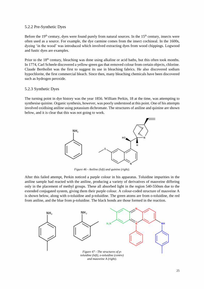
The turning point in dye history was the year 1856. William Perkin, 18 at the time, was attempting to

synthesise quinine. Organic synthesis, however, was poorly understood at this point. One of his attempts

involved oxidising aniline using potassium dichromate. The structures of aniline and quinine are shown

below, and it is clear that this was not going to work.

After this failed attempt, Perkin noticed a purple colour in his apparatus. Toluidine impurities in the

aniline sample had reacted with the aniline, producing a variety of derivatives of mauveine differing

only in the placement of methyl groups. These all absorbed light in the region 540-550nm due to the

extended conjugated system, giving them their purple colour. A colour-coded structure of mauveine A

is shown below, along with o-toluidine and p-toluidine. The green atoms are from o-toluidine, the red

from aniline, and the blue from p-toluidine. The black bonds are those formed in the reaction.

Figure 46 - Aniline (left) and quinine (right).

Figure 47 - The structures of p-

toluidine (left), o-toluidine (centre)

and mauveine A (right).

26

Perkin began mass-producing mauveine under the name aniline purple. From that point, discoveries in

dye chemistry were being made frequently. In 1858, Peter Griess discovered the processes called

diazotisation and coupling, reactions important in the synthesis of azo dyes. Ten years later, Graebe and

Liebermann produced alizarin, the first natural dye to be produced synthetically. The first azo dye was

successfully synthesised in 1880 by two English scientists, Thomas and Holliday. These are just a few

of many discoveries made in the 19th and 20th centuries concerning the chemistry of dyes.

Section 6 Structure of Dyes

6.1 Chromophores and Auxochromes

6.1.1 Basic Structure

Graebe and Liebermann, in 1868, put forward the idea of dyes containing conjugated systems. In 1876

another German, Otto Witt, suggested a general structure of dyes consisting of a conjugated system of

benzene rings with certain groups attached such as -NO2, -C=O, or -N=N-, called the chromophore, and

a polar group such as -OH or -NH2, called the auxochrome. The chromophore imparts colour to the dye

and the auxochrome deepens that colour (shifts the absorption to a longer wavelength). A couple of

examples are shown below with the chromophores coloured blue and the auxochromes red.

6.1.2 Chromophores

Dyes are often built around a central chromophore, so certain groups in the chromophore can be used

to classify the dye. Witt’s idea of the chromophore, while generally correct, took a slightly restricted

view of the possible structures it can take.

Azo dyes contain an -N=N- group in their chromophore. The groups attached to these nitrogens are

often aryl groups. With the right substituents, they can absorb a wide range of wavelengths, but are

mostly used for red, orange, and yellow dyes. Many azo dyes contain an -SO3H group as an

auxochrome. This is mostly present as -SO3- in neutral conditions so azo dyes are often produced as

salts, with the organic body of the dye being the anion.

Figure 48 – The structures of Sudan I (left) and Acridine

Orange (right).

Figure 49 - The structure of Trypan Blue, an azo dye.

27

Arylmethane dyes are divided into two main subgroups, diarylmethane dyes and triarylmethane dyes.

The backbones of these two groups are shown below.

Auramine O is currently the only commonly used diarylmethane dye. Methyl violet dyes are

triarylmethane dyes with -N(CH3)2 groups at the para position of at least two of the aryl groups.

Fuchsine dyes can have primary or secondary amines at these positions. A final example is phenol dyes,

where at least two aryl groups have -OH groups at their para positions. These phenol dyes often change

colour with pH, for example, phenolphthalein. Many of these dyes, due to their amine groups, are basic

and are often produced as salts with the organic body as the cation.

Anthraquinone dyes are built around an anthraquinone chromophore.

Anthraquinone is colourless and so auxochromes such as -OH are needed. Alizarin contains two -OH

groups on the same aryl group. This structure allows alizarin to act as a pH indicator.

Figure 50 - Diarylmethane (left) and

triarylmethane (right) general structure.

Figure 51 - The structures of Auramine O (left) and

Methyl Violet 6B (right).

Figure 52 - Anthraquinone.

Figure 53 - The structure of alizarin.

28

Xanthene-based dyes contain heterocycles, which in organic chemistry are rings containing elements

other than carbon. Xanthene itself is not particularly useful, but when it is slightly altered it becomes a

good chromophore.

The main classes of xanthene-based dyes involve substitutions of R1 and R2.

R1 R2 Dye Class

-CH= -S- Thiopyronine

-CH= -O- Pyronine

-CH= -NH-, -NMe- Acridine

-N= -S- Thiazine

-N= -O- Oxazine

-N= -NH-, -NMe- Azine Figure 55 - Table showing the dye classes in relation to the R groups.

These derivatives all have different uses. Oxazines and thiazines fade quickly in light on silks but are

useful for dyeing acrylics. Mauve, the first synthetic dye, was an azine. Fluorescein is a type of

fluorescent xanthene-based dye.

The phthalocyanines were first developed in the 20th century, more recently than the other classes. They

are the synthetic analogues of chlorophyll and haemoglobin. Phthalocyanine itself is similar in structure

to the common organic molecule, porphyrin.

Figure 54 - The structures of xanthene (left)

and a general xanthene derivative (right).

Figure 56 - The structure of fluorescein.

Figure 57 - The structures of porphyrin

(left) and phthalocyanine (right).

29

Some of the carbons of phthalocyanine can be substituted for nitrogen, and some of the outer hydrogens

for auxochromes such as -OH or -NH2 groups. This allows the colour of the dye to be finetuned.

Phthalocyanines are often produced as metal complexes, with the most common metal ion being copper.

For example, the dye Monastral Fast Blue G is simply phthalocyanine as its copper complex.

6.1.3 Auxochromes

Auxochromes usually contain a polar group with a lone pair. For example, -OH, -NH2 and -SH. These

donate electrons into the conjugated system and lengthen it, decreasing the energy difference between

the HOMO and the LUMO, causing an absorbance shift to a longer wavelength known as a

bathochromic shift.

There are certain examples which can cause a shift to a shorter wavelength, a hypsochromic shift. This

is often due to the presence of carbonyl groups next to heteroatoms. However, we will not cover the

details of how this works here.

Auxochromes can be divided into two groups, acidic and basic. This division mainly affects how a dye

is applied. Nitrogen-based auxochromes are generally basic, and oxygen and sulphur-based

auxochromes are generally acidic.

Section 7 Application and Bleaching

7.1 Application of Dyes

7.1.1 Material Structure

To understand how dyes are applied we must cover the chemical structure of certain materials.

Many fabrics, such as cotton, are made of plant fibres which are composed mainly of cellulose.

Cellulose is a polymer of glucose and the repeat unit of cellulose is shown below. The chains are stacked

on top of each other and attract each other via hydrogen bonds.

Figure 58 - The structure of

Monastral Fast Blue G.

Figure 59 - The repeat unit of cellulose.

30

In all plant-based fibres, there are substances other than cellulose present such as lignin and pectin. This

is not important, however, as the cellulose is abundant enough for a deep colour to be achieved anyway.

For example, cotton is usually 94% cellulose and most plant fibres contain at least 60%. Rayon is a type

of synthetic cellulose, and acetate rayon replaces some of the -OH groups with -OAc groups. Both of

these are commonly used in the clothing industry.

Silk, and other animal fibres such as hair, wool and leather, are mainly composed of proteins. These are

chains of amino acids joined by peptide bonds. For example, the main protein in silk is fibroin, generally

consisting of the recurring sequence of amino acids Gly-Ser-Gly-Ala-Gly-Ala.

In hair and wool, the main protein is keratin and in leather, it is collagen. Different proteins have

different amino acid sequences. The amino acids often contain acidic, basic, and polar groups which

serve as useful points for interacting with dyes molecules.

Synthetic fibres are usually polymers of some sort. Nylon, for example, is similar in structure to

proteins, with amide groups separated by carbon chains of certain lengths. The polar amide groups serve

as sites for interaction with dyes. Acrylics in their purest form are chains of hydrocarbons bearing nitrile

groups. To improve dyeability, they are often polymerised in the presence of other molecules which

add groups such as -OH. The structures of nylon-6 and a general acrylic polymer are shown below.

Some synthetic materials are difficult to dye. PET accounts for 50% of worldwide synthetic fibre

production, and while it does contain polar groups that would serve as reasonable dyeing sites, the

polymer chains are packed too close together for effective dyeing.

Tight chain packing leads to poor dyeability because dyeable fibres must be porous so that dye

molecules can enter the fibre through pores and fix themselves to the chains. If these pores are too small,

like in PET, then very few dye molecules can enter the material and the material is not easily dyed.

Figure 60 - Recurring sequence of amino acids in the protein fibroin.

Figure 61 - The repeat unit of nylon-6 (left) and an

acrylic polymer (right).

Figure 62 - The repeat unit of PET.

31

7.1.2 Dyeing Methods

There are multiple ways in which dyes can bond to fibres. These depend on both the material and the

type of dye being used.

Direct dyes are applied simply by placing the material in a hot, aqueous solution of the dye. The

temperature improves dye solubility, and direct dyes must be water-soluble. For this reason, they

usually contain ionic or polar groups. Direct dyes can be applied to most fabrics, except tightly packed

ones such as PET. The main bonding interactions are between ionic or polar groups of the fibre and the

dye. Direct dyes are often large, resulting in strong intermolecular forces of attraction (dispersion

forces) between the dye and the fibre, further strengthening its attachment.

For dyeing tightly packed synthetic fibres such as PET and acetate rayon, disperse dyes are required.

They are insoluble in water and the dyeing process involves the material being placed in a very fine,

hot suspension of the dye with a chemical called a carrier. The carrier, an example being benzyl alcohol,

transports the dye into the fibre when hot as the pores have expanded. Then, upon cooling, the dye

becomes trapped. As the dye is insoluble and the fibre tightly packed, this dyeing method creates

materials with excellent wash-fastness. Disperse dyes must be relatively small to enter the fibre.

Figure 63 - Example of an ionic interaction between an arbitrary protein and the dye Direct Blue 1.

Figure 64 - The structure of Disperse Blue 6.

32

Vat dyeing is used to apply insoluble dyes to fibres. First, a reduced form of the dye that is itself soluble

in water is applied to the material. Then, the dye is oxidised within the fibre, usually in air, into its

original, insoluble form. Because of the insolubility of vat dyes, they often have very good wash-

fastness. Indigo is a common example of a vat dye. Indigo itself is insoluble in water, but the reduced

form, indigo white, is soluble.

Reactive dyes react with the fibre and so attach themselves via covalent bonds. They are usually used

to dye plant-based fibres as they can react with the -OH groups of cellulose. The most common reactive

dyes are those based on haloheterocycles, heterocycles with attached halogens, and vinyl sulfones,

sulfonyl groups next to double bonds. The haloheterocycles are reacted with cellulose in basic

conditions. A deprotonated -OH group from cellulose attacks the heterocycle in a nucleophilic aromatic

substitution. The vinyl sulfones are formed by elimination and go on to react with cellulose in basic

conditions. A deprotonated -OH group from cellulose attacks the end carbon in a mechanism called

Michael addition.

Azo dyes are synthesised by reacting a diazonium salt with a coupling component. To apply azo dyes,

a material can be treated with a solution of the coupling component and then placed in a solution of the

diazonium salt, forming the dye on the fabric, or vice versa.

Figure 65 - The structures of Indigo White (left) and

Indigo Dye (right).

Figure 66 - Example reactions of a haloheterocycle (top) and vinyl sulfone (bottom) with cellulose, denoted Cell.

Figure 67 - Example of an azo coupling reaction.

33

7.1.3 Mordants

It is often the case that the dye alone cannot form strong enough interactions with the fibre and so has

poor fastness. This is often the case with direct dyes. To solve this issue mordants can be used. A

mordant is a substance that helps fix a dye to a material, and dyes that require mordants are called

mordant dyes.

Mordants are usually inorganic metal salts containing a metal ion with an oxidation state of at least +2,

often aluminium or iron (III). A common example is alum, KAl(SO4)2·12H2O. The metal ion can attach

to the dye via both a covalent and a coordinate bond in a process known as chelation.

When a mordant dye and metal ion chelate together, the complex formed is called a lake. Generally,

the covalent bond is to an -OH oxygen and the coordinate bond to a -C=O oxygen.

The metal can attach to more than dye molecule, and this does happen. However, not all of the metal

ions form complete complexes with the dye, as some of them form a complex with the fibre too. In this

way the dye is attached to the fibre through the metal ion.

Mordants can also alter the colours of dyes due to the presence of the metal in the conjugated system.

This is because the orbitals on the metal can affect the energy difference between the HOMO and the

LUMO.

Cellulose-based materials do not bond well to mordant dyes as they are unable to form chelations with

the metal ions. Mordant dyes are normally used to dye protein-based substances. In proteins, there are

often many hydroxyl and carboxyl groups available, with which the metal can chelate, creating a dye-

metal-fibre complex.

7.2 Bleaching

7.2.1 Bleaching Mechanism

Bleaching a material is done by destroying the chromophore of the dye. Chemical bleaches react with

the chromophore and either remove double bonds from it or break it apart completely. This interrupts

the conjugated system, meaning the dye can no longer absorb visible light, making it colourless.

Most bleaches are strong oxidising agents which can break bonds in several different ways. Some are

reducing agents which can convert double bonds into single bonds. It is also possible to cleave bonds

simply using energy, so heat and light of high enough energy such as UV light, can bleach materials.

As a result of their ability to cleave bonds and destroy certain molecules, bleaches are highly effective

at denaturing proteins. This makes them dangerous to humans, but also makes them very good

disinfectants as they can easily kill bacteria.

Figure 68 - Two examples

of metal-dye lakes.

34

7.2.2 Common Bleaches

Some of the most common bleaching agents are those based on chlorine. The first chemical bleach was

chlorine gas and since then several other bleaches containing chlorine have been discovered. Chlorine

itself is mostly used for disinfecting water but can be used to bleach wood pulp. Sodium hypochlorite,

NaClO, is often simply called bleach and is generally used in households. A mixture of calcium

hypochlorite, Ca(ClO)2, calcium hydroxide, Ca(OH)2, and calcium chloride, CaCl2, creates bleaching

powder, which has many of the same uses as sodium hypochlorite.

An example of sodium hypochlorite acting as a bleach is its reaction with an alkene. The chlorine atom

in the ClO- ion has a partial positive charge and can act as an electrophile. The double bond attacks this

atom, forming a three-membered ring as an intermediate, which is then attacked by the solvent, water,

forming a halohydrin, which can undergo further reactions. The result is that the double bond has been

broken.

The other most common bleaches are those based on peroxides. These are characterised by an O-O

peroxide bond which is easily broken, producing highly reactive species. Hydrogen peroxide, H2O2, is

used to bleach wood pulp and hair and can be used to prepare other bleaching agents. Sodium

percarbonate, Na2CO6, and sodium perborate, Na2H4B2O8, are other examples of peroxide bleaches and

have a wide range of uses.

Section 8 Specific Examples

8.1 Important Examples in Living Organisms

8.1.1 Chlorophyll

Chlorophyll is the green pigment found in plants, algae, and any other living organism that

photosynthesises. Its function is as a photoreceptor, meaning it traps light. This light then catalyses the

production of glucose via photosynthesis. The ability of chlorophyll to absorb light is very closely

related to the theory of dyes we have covered.

Chlorophyll, like any other dye, contains a large conjugated system. The chromophore is a substituted

porphyrin ring chelated with a central metal ion of magnesium. The structures of the two main types

of chlorophyll, A and B, are shown below. The only difference is that in chlorophyll A, the R group is

-CH3, and in chlorophyll B, it is -CHO.

Figure 69 - Reaction of sodium hypochlorite with an alkene.

Figure 70 - The structure of chlorophyll.

35

The extended conjugated system is clear, stretching over the porphyrin and some of the attached groups.

The wavelength of light absorbed is further altered by the magnesium, whose orbitals can interact with

those of the conjugated system.

Chlorophyll A and B work together in plants to absorb a large range of the visible spectrum, allowing

sunlight to be used as a source of energy. Wavelengths that one type fails to absorb are often made up

for by the other. However, there is still a gap in the absorbance spectrum from 500nm to 600nm, which

corresponds to green light, causing the green colour of chlorophyll.

In photosynthesis, energy from sunlight is absorbed by the conjugated system, leading to the excitation

of an electron in chlorophyll. This electron can now be easily transferred to other molecules and a long

chain of electron transfers leads to the transfer of an electron to a CO2 molecule, reducing it, and the

removal of an electron from H2O molecule. Chlorophyll is bound to the back of a large, complex protein

which positions it perfectly to react with any nearby water and carbon dioxide quickly and efficiently.

As chlorophyll has such a strong absorbance in the visible spectrum, it masks the colours of other

molecules present in leaves. This can be seen in autumn when the chlorophyll decays, allowing the

oranges and reds of carotenoids to be seen. Also, when leaves are cooked, they become slightly more

yellow as the magnesium is removed from the chlorophyll molecules.

8.1.2 Retinal

Retinal is found in the eye and is a molecule that allows humans to see. It undergoes a cycle of chemical

changes, together with the protein opsin, called the visual cycle. The retinal molecule contains an

extended conjugated system. The structure of this conjugated system is why we see the wavelengths of

light that we do, and not, for example, ultraviolet light.

Retinal is very similar in structure to β-carotene. As humans cannot synthesise retinal, we must ingest

β-carotene through foods such as carrots, which can then be cleaved to give vitamin A (retinol) and

through oxidation, retinal.

Figure 71 - The structure of all-trans-retinal.

Figure 72 - A summary of the conversion of 𝛽-carotene to all-trans-retinal.

36

At a certain point in the visual cycle, a molecule of 11-cis-retinal binds to the protein opsin via a lysine

residue. This new retinal-opsin molecule is called rhodopsin and has a strong absorbance in the region

of 400 𝑛𝑚 − 700 𝑛𝑚, depending on the type of opsin. When a photon of the right wavelength is

absorbed by the rhodopsin, the energy goes converts the double bond between the 11th and 12th carbon

into a single bond, meaning it is free to rotate. When it has rotated through 180°, the double bond

reforms, now in a trans configuration. The retinal is now all-trans-retinal, which does not fit the opsin

binding site well, so the link between the retinal and the opsin weakens, and several fast reactions occur

before they detach completely. This sudden movement is transferred through the protein to the

membrane it is attached to, and eventually is picked up by nerve cells in the optic nerve which send a

signal to the brain. The brain detects these and so we can see. The all-trans-retinal can undergo a series

of enzyme-catalysed changes to reform 11-cis-retinal and the cycle repeats.

There are three types of rhodopsin, each with a slightly different structure, that absorb at different

wavelengths. The three are responsible for light in the red, green, and blue portions of the visible

spectrum and all three working together results in our ability to see the colours that we do.

8.2 pH Indicators

8.2.1 General Mechanism

Certain chemicals appear different colours in acidic and basic conditions and can, therefore, be used as

pH indicators. The pH of a solution is defined as the negative logarithm, base ten, of the concentration

of H3O+ ions.

𝑝𝐻 = − log10[𝐻3𝑂+]

The colour change is usually caused by the dissociation of an H+ ion from the indicator. The neutral,

𝐻𝐼𝑛, and deprotonated, 𝐼𝑛−, forms of the indicator are in equilibrium with each other.

𝐻𝐼𝑛 + 𝐻2𝑂 ⇌ 𝐼𝑛− + 𝐻3𝑂+

The equilibrium constant for this reaction is called the acid dissociation constant, Ka. Another constant,

the pKa, is defined as the negative logarithm, base ten, of the acid dissociation constant. The pKa values

of different indicators can be found in data books.

𝐾𝑎 =[𝐻3𝑂+][𝐼𝑛−]

[𝐻𝐼𝑛], 𝑝𝐾𝑎 = − log10 𝐾𝑎

Figure 73 - A simplified diagram of the visual cycle. 11-cis-retinal (top left) is converted into rhodopsin (top right), then

straightened (bottom right), then cleaved to all-trans-retinal (bottom left) and then converted back into 11-cis retinal.

37

There is an equation linking the concentration of 𝐻𝐼𝑛 and 𝐼𝑛−, the pH of the solution and the pKa of

the indicator (the pKIn) called the Henderson-Hasselbalch equation. It can be derived by taking

logarithms of both sides of the Ka equation.

𝑝𝐻 = 𝑝𝐾𝑎 + log10

[𝐼𝑛−]

[𝐻𝐼𝑛]

From this equation, it can be deduced that if the pH is equal to pKIn, the concentration of 𝐼𝑛− is equal

to the concentration of 𝐻𝐼𝑛. If the pH is below pKIn, the concentration of 𝐼𝑛− is less than that of 𝐻𝐼𝑛.

If the pH is above pKIn, the concentration of 𝐼𝑛− is greater than that of 𝐻𝐼𝑛.

For a weak acid indicator where 𝐻𝐼𝑛 has a colour, say red, and 𝐼𝑛− a different colour, say blue, then

the colour changes can be estimated. At a pH equal to pKIn, the concentrations of 𝐻𝐼𝑛 and 𝐼𝑛− are

equal, so the solution is purple. At a lower pH, the concentration of 𝐼𝑛− is smaller than the concentration

of 𝐻𝐼𝑛. As the pH scale is logarithmic, after about one unit of pH, the concentration of 𝐻𝐼𝑛 is already

about ten times larger than that of 𝐼𝑛−, so the solution is red. At a higher pH than pKIn, the concentration

of 𝐻𝐼𝑛 is smaller than the concentration of 𝐼𝑛−, so the solution is blue.

For any pH indicator, there is a pKIn and a range either side of this in which the solution is undergoing

a colour change. The best indicators have a clear colour change and a small range over which the colour

is changing.

8.2.2 Common Examples and Acid-Base Titrations

A universal indicator gives an approximate measure of pH by having a wide range of colours in different

pH values. Universal indicators are composed of a mixture of several indicators, each specifically

selected for their pKIn and colour change. When the correct indicators are mixed, a solution can be

created that steadily changes through multiple different colours as the pH is altered, which is very useful

for qualitative analysis.

The most common universal indicator is composed of a mixture of thymol blue, methyl orange, methyl

red, bromothymol blue and phenolphthalein. This mixture results in a colour change from red in strong

acid to violet in strong alkali, following the visible spectrum.

Indicators are often used in acid-base titrations, and the two most common indicators for this are

phenolphthalein and methyl orange. Phenolphthalein loses two protons between pH 8.2 and 10.0, going

from the colourless 𝐻2𝐼𝑛 to the bright pink 𝐼𝑛2− in this range. Methyl orange changes between pH 3.2

and pH 4.4 from the red zwitterion, 𝐻𝐼𝑛, to the yellow 𝐼𝑛−.

Figure 74 - The structures of phenolphthalein below pH 8.2 (left) and above pH 10.0

(right).

38

When choosing an indicator for a titration, it must change colour at a pH near the equivalence point,

the point where the two substances have been mixed in equal proportions. The shape of the titration

curve allows for a large variation in pH from the equivalence point with minimal loss of accuracy. For

this reason, both phenolphthalein and methyl orange change colour close enough to pH 7 that they can

be used for strong acid-strong base titrations. But for weak acid-strong base titrations, the equivalence

point is at a higher pH, so methyl orange is no longer a valid indicator to use. The opposite is true for

strong acid-weak base titrations, so phenolphthalein is not valid. For weak acid-weak base titrations,

the shape of the titration curve is such that neither of these indicators are useful.

Section 9 Concluding Remarks

This exploration of the chemistry of dyes has taken us through many branches of chemistry from

quantum mechanics and atomic and molecular orbitals to biochemistry and acid-base indicators. It is

clear that the study of dyes is a rich field full of interest and that there is a lot to be gained from studying

them.

Dyes not only hold an important place in chemistry but also our lives. All the clothes we wear every

day have most likely been dyed or bleached in some way. Then there is the fabric on the furniture, the

food dyes in the cupboard, the list goes on. Even outside, away from man-made objects, the landscape

is filled with the vibrant colours of plant life. It is impossible to escape the importance of dyes in our

daily lives.

Section 10 Bibliography

10.1 Section 2 Quantum Mechanics

Branson, J. (2013). Black Body Radiation. [online] Available at:

https://quantummechanics.ucsd.edu/ph130a/130_notes/node48.html [Accessed 23 Apr. 2020].

Sherrill, D. (2006). The Ultraviolet Catastrophe. [online] Available at:

http://vergil.chemistry.gatech.edu/notes/quantrev/node3.html [Accessed 23 Apr. 2020].

(2005). Annus Mirabilis Papers. [online] Available at:

https://en.wikipedia.org/wiki/Annus_Mirabilis_papers [Accessed 23 Apr. 2020].

Calbreath, D. and Baxter, W. (2013). Photoelectric Effect. [online] Available at:

https://courses.lumenlearning.com/cheminter/chapter/photoelectric-effect/ [Accessed 23 Apr. 2020].

The Editors of Encyclopaedia Britannica. (2018). Photoelectric Effect. [online] Available at:

https://www.britannica.com/science/photoelectric-effect [Accessed 23 Apr. 2020].

Keeler, J. and Wothers, P. (2008). Chemical Structure and Reactivity. ed. 2. Oxford: Oxford

University Press, pp. 37-38, 663-678.

Figure 75 - The structures of methyl orange below pH 3.2 (left) and above pH 4.4 (right).

39

Sherrill, D. (2003). Postulates of Quantum Mechanics. [online] Available at:

http://vergil.chemistry.gatech.edu/notes/intro_estruc/node4.html [Accessed 24 Apr. 2020].

(2005). Momentum Operator. [online] Available at:

https://en.wikipedia.org/wiki/Momentum_operator [Accessed 24 Apr. 2020].

10.2 Section 3 Atomic and Molecular Orbitals

Trefil, J and Bertsch, G. (20120). Atom. [online] Available at:

https://www.britannica.com/science/atom [Accessed 24 Apr. 2020].

(2003). Geiger-Marsden Experiment. [online] Available at:

https://en.wikipedia.org/wiki/Geiger%E2%80%93Marsden_experiment [Accessed 24 Apr. 2020].

Knott, T. (2001). Bohr Model. [online] Available at: https://en.wikipedia.org/wiki/Bohr_model

[Accessed 24 Apr. 2020].

Keeler, J. and Wothers, P. (2008). Chemical Structure and Reactivity. ed. 2. Oxford: Oxford

University Press, pp. 36-68, 100-122, 132-136.

(2001). Uncertainty Principle. [online] Available at:

https://en.wikipedia.org/wiki/Uncertainty_principle [Accessed 24 Apr. 2020].

Hopkins, B. (2001). Spherical Coordinate System. [online] Available at:

https://en.wikipedia.org/wiki/Spherical_coordinate_system [Accessed 24 Apr. 2020].

Hanson, D and Harvey, E and Sweeney, R and Zielinski, T. (2020). The Schrödinger Wave Equation

for the Hydrogen Atom. [online] Available at:

https://chem.libretexts.org/Bookshelves/Physical_and_Theoretical_Chemistry_Textbook_Maps/Map

%3A_Physical_Chemistry_for_the_Biosciences_(Chang)/11%3A_Quantum_Mechanics_and_Atomic

_Structure/11.10%3A_The_Schr%C3%B6dinger_Wave_Equation_for_the_Hydrogen_Atom

[Accessed 24 Apr. 2020].

(2001). Molecular Orbitals. [online] Available at:

https://wps.prenhall.com/wps/media/objects/3081/3155729/blb0907.html [Accessed 15 Jun. 2020].

(2015). Molecular Orbital Theory. [online] Available at: https://opentextbc.ca/chemistry/chapter/8-4-

molecular-orbital-theory/ [Accessed 15 Jun. 2020].

10.3 Section 4 Bonding in Organic Molecules and Colour

Keeler, J. and Wothers, P. (2008). Chemical Structure and Reactivity. ed. 2. Oxford: Oxford

University Press, pp. 149-158, 167-177.

Clayden, J. and Greeves, N. and Warren, S. (2001). Organic Chemistry. ed. 2. Oxford: Oxford

University Press, pp. 143-149.

Cruzan, J. (2019). Hybrid Orbitals. [online] Available at:

https://xaktly.com/OrbitalHybridization.html [Accessed 16 Jun. 2020].

40

Reusch, W. (2013). Visible and Ultraviolet Spectroscopy. [online] Available at:

https://www2.chemistry.msu.edu/faculty/reusch/VirtTxtJml/Spectrpy/UV-Vis/spectrum.htm

[Accessed 16 Jun. 2020].

Chieh, C. (2020). Bond Lengths and Energies. [online] Available at:

https://chem.libretexts.org/Bookshelves/Physical_and_Theoretical_Chemistry_Textbook_Maps/Suppl

emental_Modules_(Physical_and_Theoretical_Chemistry)/Chemical_Bonding/Fundamentals_of_Che

mical_Bonding/Chemical_Bonds/Bond_Lengths_and_Energies [Accessed 5 May 2020].

10.4 Section 5 Terminology and History of Dyes

(2002). Indigo Dye. [online] Available at: https://en.wikipedia.org/wiki/Indigo_dye [Accessed 7 May

2020].

(2002). Tyrian Purple. [online] Available at: https://en.wikipedia.org/wiki/Tyrian_purple [Accessed 7

May 2020].

Driessen, K. Early Use of Natural Dyes in Textiles. [online] Available at:

http://www.quilthistory.com/dye.htm [Accessed 7 May 2020].

(2014). Justinian I. [online] Available at: https://www.ancient.eu/image/3341/justinian-i/ [Accessed 7

May 2020].

(2005). Betanin. [online] Available at: https://en.wikipedia.org/wiki/Betanin [Accessed 7 May 2020].

Jones, M. (2016). The History and Chemistry of Dyes. YouTube video added by Adams State

University. [online] Available at:

https://www.youtube.com/watch?v=DiXnBOA3Mag&list=WL&index=68&t=0s [Accessed 7 May

2020].

Manske, M. (2001). Carl Wilhelm Scheele. [online] Available at:

https://en.wikipedia.org/wiki/Carl_Wilhelm_Scheele [Accessed 7 May 2020].

(2004). Bleach. [online] Available at: https://en.wikipedia.org/wiki/Bleach [Accessed 7 May 2020].

(2001). Quinine. [online] Available at: https://en.wikipedia.org/wiki/Quinine [Accessed 7 May 2020].

(2003). Aniline. [online] Available at: https://en.wikipedia.org/wiki/Aniline [Accessed 7 May 2020].

Cova, T. and Alberto, A. and Seixas de Melo, J. (2017). Reconstructing the Historical Synthesis of

Mauveine from Perkin and Caro: Procedure and Details. [online] Available at:

https://www.nature.com/articles/s41598-017-07239-z [Accessed 7 May 2020].

(2003). Mauveine. [online] Available at: https://en.wikipedia.org/wiki/Mauveine [Accessed 7 May

2020].

(2016). The Evolution of Textile Dyes: History and Development. [online] Available at:

http://www.keycolour.net/blog/the-evolution-of-textile-dyes-history-and-development/ [Accessed 7

May 2020].

41

Druding, S. (1982). Dye History from 2600 BC to the 20th Century. [online] Available at:

http://www.straw.com/sig/dyehist.html [Accessed 7 May 2020].

(2007). Peter Griess. [online] Available at: https://en.wikipedia.org/wiki/Peter_Griess [Accessed 7

May 2020].

Kiron, M. (2020). What is Colour Fastness? [online] Available at:

https://textilelearner.blogspot.com/2011/12/what-is-color-fastness-classification.html [Accessed 12

May 2020].

10.5 Section 6 Structure of Dyes

Abrahart, E. and Stothers, J. (2020). Dye. [online] Available at:

https://www.britannica.com/technology/dye [Accessed 9 May 2020].

(2005). Sudan I. [online] Available at: https://en.wikipedia.org/wiki/Sudan_I [Accessed 9 May 2020].

(2006). Acridine Orange. [online] Available at: https://en.wikipedia.org/wiki/Acridine_orange

[Accessed 9 May 2020].

Bathochromic Shift. [online] Available at:

http://www.chem.ucla.edu/~harding/IGOC/B/bathochromic_shift [Accessed 9 May 2020].

(2005). Azo Dye. [online] Available at: https://en.wikipedia.org/wiki/Azo_dye [Accessed 9 May

2020].

Lillie, R. (2019). Arylmethane Dyes. [online] Available at:

http://stainsfile.info/dyes/class/clsarylm.htm [Accessed 10 May 2020].

(2007). Triarylmethane Dye. [online] Available at: https://en.wikipedia.org/wiki/Triarylmethane_dye

[Accessed 9 May 2020].

(2003). Methyl Violet. [online] Available at: https://en.wikipedia.org/wiki/Methyl_violet [Accessed 11

May 2020].

(2005). Auramine O. [online] Available at: https://en.wikipedia.org/wiki/Auramine_O [Accessed 10

May 2020].

(2005). Fuchsine. [online] Available at: https://en.wikipedia.org/wiki/Fuchsine [Accessed 11 May

2020].

(2003). Alizarin. [online] Available at: https://en.wikipedia.org/wiki/Alizarin [Accessed 12 May

2020].

(2010). Anthraquinone Dyes. [online] Available at: https://en.wikipedia.org/wiki/Anthraquinone_dyes

[Accessed 9 May 2020].

(2004). Fluorescein. [online] Available at: https://en.wikipedia.org/wiki/Fluorescein [Accessed 12

May 2020].

42

(2005). Xanthene. [online] Available at: https://en.wikipedia.org/wiki/Xanthene [Accessed 9 May

2020].

(2004). Phthalocyanine. [online] Available at: https://en.wikipedia.org/wiki/Phthalocyanine

[Accessed 11 May 2020].

(2015). How do Auxochrome Groups Work? [online] Available at:

https://chemistry.stackexchange.com/questions/29453/how-do-auxochrome-groups-work [Accessed 9

May 2020].

10.6 Section 7 Application and Bleaching

Abrahart, E. and Stothers, J. (2020). Dye. [online] Available at:

https://www.britannica.com/technology/dye [Accessed 13 May 2020].

Stevens, M. and Preston, J. (2016). Major Industrial Polymers. [online] Available at:

https://www.britannica.com/topic/industrial-polymers-468698/Phenol-formaldehyde#ref76470

[Accessed 13 May 2020].

(2009). Cellulose Fibre. [online] Available at: https://en.wikipedia.org/wiki/Cellulose_fiber

[Accessed 13 May 2020].

Das, A. (2020). Structure of Cotton Fibre. [online] Available at:

https://textilelearner.blogspot.com/2013/04/structure-of-cotton-fiber.html [Accessed 13 May 2020].

(2007). Fibroin. [online] Available at: https://en.wikipedia.org/wiki/Fibroin [Accessed 13 May 2020].

(2009). Direct Blue 1. [online] Available at: https://en.wikipedia.org/wiki/Direct_Blue_1 [Accessed

14 May 2020].

(2016). Dyes and Dyeing. [online] Available at:

https://www.flinnsci.com/api/library/Download/c46ad9cfbff64e9cae7caf3aed645692 [Accessed 14

May 2020].

Kiron, M. (2020). Introduction of Direct Dyes. [online] Available at:

https://textilelearner.blogspot.com/2011/02/defination-classification-application_2111.html [Accessed

14 May 2020].

Kiron, M. (2020). Disperse Dye. [online] Available at:

https://textilelearner.blogspot.com/2012/01/disperse-dye-history-of-disperse-dye.html [Accessed 14

May 2020].

Kiron, M. (2020). Different Types of Dyes with Chemical Structure. [online] Available at:

https://textilelearner.blogspot.com/2015/01/differentK-types-of-dyes-with-chemical.html [Accessed

14 May 2020].

(2002). Indigo Dye. [online] Available at: https://en.wikipedia.org/wiki/Indigo_dye [Accessed 12 May

2020].

43

(2015). Vat Dye. [online] Available at: https://www.britannica.com/science/vat-dye [Accessed 8 Jun.

2020].

(2020). Reactive Dye. [online] Available at: https://www.britannica.com/technology/reactive-dye

[Accessed 8 Jun. 2020].

(2005). Reactive Dye. [online] Available at: https://en.wikipedia.org/wiki/Reactive_dye [Accessed 8

Jun. 2020].

Kiron, M. (2020). Classification of Reactive Dyes. [online] Available at:

https://textilelearner.blogspot.com/2012/01/classification-of-reactive-dyes.html [Accessed 8 Jun.

2020].

(2019). Vinyl Sulfone Dyes. [online] Available at: https://en.wikipedia.org/wiki/Vinyl_sulfone_dyes

[Accessed 8 Jun. 2020].

(2019). Mordants. [online] Available at: http://stainsfile.info/theory/mordant.htm [Accessed 9 Jun.

2020].

(2020). How Does Bleach Whiten Clothes and Why Does it Ruin Clothes if Too Much is Applied?

[online] Available at: http://scienceline.ucsb.edu/getkey.php?key=551 [Accessed 8 Jun. 2020].

Ashenhurst, J. (2020). Conjugation and Colour (+How Bleach Works). [online] Available at:

https://www.masterorganicchemistry.com/2016/09/08/conjugation_and_color/ [Accessed 9 Jun.

2020].

(2004). Bleach. [online] Available at: https://en.wikipedia.org/wiki/Bleach [Accessed 9 Jun. 2020].

10.7 Section 8 Specific Examples

May, P. Chlorophyll. [online] Available at:

http://www.chm.bris.ac.uk/motm/chlorophyll/chlorophyll_h.htm [Accessed 11 Jun. 2020].

Biggs, T. and McPhail, S. and Nassau, K. Green Plants and Chlorophyll. [online] Available at:

http://www.webexhibits.org/causesofcolor/7A.html [Accessed 11 Jun. 2020].

Retinal. [online] Available at: https://www.ch.ic.ac.uk/vchemlib/mim/bristol/retinal/retinal_text.htm

[Accessed 12 Jun. 2020].

(2003). Rhodopsin and the Eye. [online] Available at:

http://www.chm.bris.ac.uk/webprojects2003/rogers/998/Rhoeye.htm [Accessed 12 Jun. 2020].

(2001). Acid-Base Indicators and Titrations. [online] Available at:

https://www.ch.ic.ac.uk/vchemlib/course/indi/ [Accessed 12 Jun. 2020].

How Do pH Indicators Work? [online] Available at:

https://scilearn.sydney.edu.au/fychemistry/demonstrations/worksheets/5.8_answers.pdf [Accessed 12

Jun. 2020].

44

(2005). Universal Indicator. [online] Available at: https://en.wikipedia.org/wiki/Universal_indicator

[Accessed 12 Jun. 2020].

Clark, J. (2002). Acid-Base Indicators. [online] Available at:

https://www.chemguide.co.uk/physical/acidbaseeqia/indicators.html [Accessed 12 Jun. 2020].

(2003). Phenolphthalein. [online] Available at: https://en.wikipedia.org/wiki/Phenolphthalein

[Accessed 12 Jun. 2020].

(2004). Methyl Orange. [online] Available at: https://en.wikipedia.org/wiki/Methyl_orange [Accessed

12 Jun. 2020].