creating a test validated structural dynamic finite ... · the ground vibration test-validated...
TRANSCRIPT

1American Institute of Aeronautics and Astronautics
Creating a Test Validated Structural Dynamic Finite Element Model of the X-56A Aircraft
Chan-gi Pak1 and Samson Truong2
NASA Armstrong Flight Research Center, Edwards, CA 93523-0273
Small modeling errors in the finite element model will eventually induce errors in the structural flexibility and mass, thus propagating into unpredictable errors in the unsteady aerodynamics and the control law design. One of the primary objectives of the Multi Utility Technology Test-bed, X-56A aircraft, is the flight demonstration of active flutter suppression, and therefore in this study, the identification of the primary and secondary modes for the structural model tuning based on the flutter analysis of the X-56A aircraft.The ground vibration test-validated structural dynamic finite element model of the X-56A aircraft is created in this study. The structural dynamic finite element model of the X-56A aircraft is improved using a model tuning tool. In this study, two different weight configurations of the X-56A aircraft have been improved in a single optimization run.Frequency and the cross-orthogonality (mode shape) matrix were the primary focus for improvement, while other properties such as center of gravity location, total weight, and off-diagonal terms of the mass orthogonality matrix were used as constraints. The end result was a more improved and desirable structural dynamic finite element model configuration for the X-56A aircraft. Improved frequencies and mode shapes in this study increased average flutter speeds of the X-56A aircraft by 7.6% compared to the baseline model.
NomenclatureA = area of bar cross sectionABFF = anti-symmetric body freedom flutterAFRC = Armstrong Flight Research CenterAFRL = Air Force Research LaboratoryAMLGFA = anti-symmetric main landing gear forward and aftAMLGL = anti-symmetric main landing gear lateralARMD = Aeronautics Research Mission DirectorateAW1B = anti-symmetric wing first bendingAW1T = anti-symmetric wing first torsionAW2B = anti-symmetric wing second bendingAW2T = anti-symmetric wing second torsionAW3B = anti-symmetric wing third bendingAWBTF = anti-symmetric wing bending torsion flutterAWFA = anti-symmetric wing forward and aftAWL = anti-symmetric winglet BoomH = boom horizontalBoomV = boom verticalCG = center of gravityDOT = design optimization toolsE = Young’s modulusEFEW = Empty Fuel Empty Water
1Research Manager, Aerospace Engineer, Aerostructures Branch, P.O. Box 273 Edwards, California/Mailstop 48201A, Senior Member AIAA.2Aerospace Engineer, Aerostructures Branch, P.O. Box 273 Edwards, California/Mailstop 48201A, Member AIAA.
https://ntrs.nasa.gov/search.jsp?R=20140010281 2020-05-30T23:38:53+00:00Z

2American Institute of Aeronautics and Astronautics
FE = finite elementFFFW = Full Fuel Full Waterf = frequencyG = Shear modulusGVT = ground vibration testI1 = area moment of inertia of bar with respect to plane 2I2 = area moment of inertia of bar with respect to plane 1J = objective functionJk = performance indicesK2 = spring constant in direction 2K3 = spring constant in direction 3K4 = spring constant in direction 4LMSW = Lockheed Martin Skunk Works�� = analytical mass matrix obtained from Nastran�� = Orthogonal matrixMAC = modal assurance criteriam = number of modes to be use in system equivalent reduction expansion processNASA = National Aeronautics and Space AdministrationNLGFA = nose landing gear forward and aftNLGL = nose landing gear lateraln = number of modes for model tuningnAD = number of A-set degrees of freedom nMD = number of measured (or master) degrees of freedomO3 = Object-Oriented OptimizationPOH = previous optimization history�� = cross-orthogonality matrixSBFF = symmetric body freedom flutterSMLGFA = symmetric main landing gear forward and aftSMLGL = symmetric main landing gear lateralSWL = symmetric winglet SW1B = symmetric wing first bendingSW1T = symmetric wing first torsionSW2B = symmetric wing second bendingSW2T = symmetric wing second torsionSW3B = symmetric wing third bendingSWBTF = symmetric wing bending torsion flutterSWFA = symmetric wing forward and aftV = velocity����� = eigen matrix obtained from Nastran modal analysis� = intermediate matrix to compute ���� = eigen matrix, corresponds to master degrees of freedom�� = eigen matrix, corresponds to slave degrees of freedom
I. IntroductionNE of the major goals of the Fundamental Aeronautics program under the National Aeronautics and Space Administration (NASA) Aeronautics Research Mission Directorate (ARMD) is to develop a cutting-edge
technology for higher performance lighter weight aircraft. Higher performance includes energy efficiency andoperability technologies that enable advanced airframe and engine systems. Removing weight from an aircraft usually results in reduced stiffness; and therefore, increased flexibility. The increased flexibility creates an aircraft that is more susceptible to aeroelastic phenomena such as flutter, divergence, buzz, buffet, and gust response. Therefore, structural weight reduction is constrained by these adverse aeroelastic phenomena.
The ability for flexible motion control, such as gust load alleviation and active flutter suppression, will help in opening the new design space for lighter weight aircraft, which will increase fuel efficiency and help with noise reduction. Many active aeroelastic controller designs have been developed and proven analytically. In some cases wind-tunnel tests have been performed to demonstrate these designed active controllers. Based on the maturation of
O

3American Institute of Aeronautics and Astronautics
active aeroelastic controls, it is time to perform an actual flight demonstration of these active controllers. However, there has been limited testing on active flutter suppression technology due to the high risk of vehicle loss.
An open, non-propriety, unmanned aerial vehicle (UAV) called the Multi Utility Technology Test-bed (X-56A),as shown in Fig. 1, has been developed by the Air Force Research Laboratory (AFRL) (Wright-Patterson Air Force Base, Ohio) for relatively high risk aeroelastic flight demonstrations and future research. If a flight goes beyond flutter boundaries and a wing fails, then the X-56A aircraft is fitted with a center body mounted ballistic parachute recovery system. Sharing the same goal to design a lighter weight aircraft by suppressing associated aeroelastic instabilities using an active control, has led to a joint collaboration between NASA and the AFRL. The AFRL will provide the X-56A aircraft, ground control stations, analytical models, as well as ground and flight-test data to NASA. After the first flight test with flexible wings, the valuable AFRL’s assets, two reusable center bodies, one rigid wing, three flexible wings, and ground control stations, will stay at NASA Armstrong Flight Research Center (AFRC) (Edwards, California) for future technology demonstrations, such as the NASA designed lighter weight wing with curvilinear spars and ribs, the Northrop Grumman (Falls Church, Virginia) designed flying wing, and/or the Boeing (Chicago, Illinois) designed joined wing, as shown in Fig 2. Furthermore, Lockheed Martin Skunk Works (LMSW) in Palmdale, California will provide NASA the finite element models and the ground vibration test data for this research project.
The X-56A aircraft has a wing span of 28 ft and a weight between 200–480 lb, depending on its configuration.1This aircraft is powered by twin JetCat P400 turbojet engines (JetCat USA, Tehachapi, California) and configured for easy wing replacement. The design also includes a hard point on the center upper deck of the aft fuselage that can either be adapted to house a third engine or the boom for a joined wing, thereby enabling testing of more advanced aerodynamic concepts. A ground vibration test was completed on December 17, 2012, and test data has been provided to NASA for model validations.
Modern aircraft make extensive use of composite materials in order to reduce weight. Aircraft aeroservoelastic models have significant levels of model parameter uncertainty due to the composite manufacturing process. In an attempt to mitigate this, ground vibration test (GVT) data can be used to tune a model and help to improve its accuracy over a wider range of operating environments. This tuning and adaption procedure has become an accepted and necessary step in making models more reliable; however, it cannot handle or eliminate all uncertainties in afinite element (FE) model. In order to minimize the uncertainties in aeroelastic as well as aeroservoelastic response computations, the structural dynamic model, the unsteady aerodynamic model, and the actuator model should be validated with respect to the corresponding test data.2,3 Small modeling errors in a FE model will eventually induce errors in the structural flexibility and mass, thus propagating into unpredictable errors in the unsteady aerodynamics and the control law design. Tuning a FE model using measured data to minimize the modeling uncertainties is a challenging task in the area of structural dynamics.
Supporting the ARMD guidelines, NASA AFRC has developed a computer code for FE model tuning2,4 using the Object-Oriented Optimization (O3) tool5 together with Nastran (MSC Software Corporation, Newport Beach, California),6 a FE analysis computer software program. Three optimizer algorithms have been incorporated into the O3 tool: design optimization tools (DOT)7 based on a gradient-based algorithm, the genetic algorithm (GA),8 which is a class of stochastic and global optimization, and big-bang big-crunch algorithms.9-12 This O3 tool, as shown in Fig. 3, was crucial in the development of a multidisciplinary design, analysis, and optimization (MDAO) tool13 and an unsteady aerodynamic model tuning tool.3
The primary objective of this study is to obtain the GVT-validated structural dynamic finite element model of the X-56A aircraft. Based on the validated model, flutter boundaries will be computed again and compared with results obtained from the non-validated model. The secondary objective of this study is to improve and extend the previously developed structural dynamic finite element model tuning tool2 and demonstrate this tool using the X-56A aircraft as a sample case.
II. Optimization Theoretical BackgroundIn the FE model tuning tool, the user will choose an optimization algorithm, define the continuous as well as the
discrete design variables with side constraints, starting values, and scaling factors; and provide script and data file names for each performance index. Communication between the O3 tool and each analysis sub-module will be performed through the use of design variables and performance indices. Once the O3 tool is executed, design variables will be created and saved in an external data file. This data file cannot be shared with other analysis sub-modules; and therefore, a script command will make a copy of this data file first. Script commands for each performance index will perform the following tasks:
� prepare data for analysis program (pre-processor module);

4American Institute of Aeronautics and Astronautics
� submit analysis job (analyzer module); and� read result files, compute the required performance index value, and save it (post-processor module).
Analysis sub-modules of the extended model tuning tool are explained in this section. Blocks in Fig. 3 can be categorized into three modules: the pre-processor, the analyzer, and the post-processor modules. The pre-processor module (Update Nastran input deck block) in Fig. 3 is used to create and update input files based on the design variable values provided by the O3 tool before executing the analyzer module. The analyzer module (Nastran modal analysis block) in Fig. 3 can be a commercial and/or the in-house codes for a specific discipline. The script commands will execute the analyzer module automatically. The postprocessor module is used to post-process the Nastran output file, which is computed from the analyzer module, and it automatically computes the performance indices. Several sub-modules were developed for the structural dynamic FE model tuning.
A. Weight Sub-module A weight generator in Nastran code and measured test data are used to compute the maximum ten performance
indices associated with the total weight, center of gravity (CG) locations, and the moment of inertias. Note that the G in the subscripts for the following variables displayed represents the test-measured data value as shown in Eqs. (1)–(10):
J = ������� ��(Total weight) (1)
J� = ������� ��(x CG location) (2)
J� = ������� ��(y CG location) (3)
J� = ������� ��(z CG location) (4)
J� = ������������� ��(Ixx at CG) (5)
J� = ������������� ��(Iyy at CG) (6)
J = ��!!��!!��!!� ��(Izz at CG) (7)
J" = ������������� ��(Ixy at CG) (8)
J# = ���!���!���!� ��(Iyz at CG) (9)
J $ = ��!���!���!�� ��(Izx at CG) (10)
B. Mass Orthogonality Sub-moduleThis sub-module computes each off-diagonal term of the orthogonality matrix using Eq. (11):
�� = ��%���& ���%��� (order = n × n) (11)
In Eq. (11), the order of a reduced order mass matrix, ��, is based on the A-set degrees of freedom6 and computed using the System Equivalent Reduction Expansion Process (SEREP) shown in Eqs. (12) and (13),14

5American Institute of Aeronautics and Astronautics
�� = ��&� (order = nAD × nAD) (12)
� = '����& ����(� ����& (order = m × nAD) (13)
where the matrix, ���� (order = nAD × m), is an eigen matrix obtained from Nastran modal analysis, and m and nADare the number of modes to be use in the SEREP and the number of A-set degrees of freedom, respectively.Expanded GVT mode shape, �%��� , is also computed using SEREP as follows:
Reorder the matrix, ���� , then ���� ) *���� + and the matrix, �%��� (order = nAD × n), will become Eq. (14),
�%��� = ,��'��& ��(� ��&
�-'��& ��(� ��&
.�/ %� (14)
where matrices, �� (order = nMD × m) and �� (order = (nAD - nMD) × m), are the master and slave eigen matrices.The nMD and n are the measured (or master) degrees of freedom and the number of modes for model tuning,respectively; and �/ %� (nMD × n) is the measured eigen matrix obtained from GVT.
The number of performance indices (off-diagonal term square of matrix �� ),
J0 = �� 12� 4 5 6 4 & 6 = 1, 2, … , n (15)
computed in this sub-module is
L� = ;<�;� (16)
where k = 11, … , 10 + L�. In the previous version of model tuning tool, only one performance index,
J = > > �� ?@AB@C?DEB?CE (17)
was defined for mass orthogonality. The extended version of the model tuning tool required a significant number of performance indices, since each
individual off-diagonal term, as shown in Eqs. (15) and (16), were performance indices instead of using a single norm value of off-diagonal terms as in Eq. (17), which was used in the previous version of the model tuning tool.2,4
With the extended version, it was much easier to improve each off-diagonal term element as opposed to the previous version.
C. Frequency Sub-modulePerformance indices associated with the i-th frequency error are computed from Eq. (18),
J0 = �FG�FG�FG� ��k= 11+LH, … , 10+ L�+m (18)
where f1 and�f1% �are the i-th numerical and measured frequencies. The m performance indices (number of modes to be matched) are computed in this sub-module. Similarly, the previous version of the model tuning tool had only one performance index for frequency error and was defined as Eq. (19):
J = > �FG�FG�FG� ��;1C (19)

6American Institute of Aeronautics and Astronautics
D. Mode Shape Sub-moduleIn the previous version of the model tuning tool, numerical mode shapes were improved to minimize mode shape
error at sensor locations using a single performance index. In the extended version, each off-diagonal term of the cross-orthogonality matrix is computed using Eq. (20):
�� = ��%���& ������ (20)
The number of performance indices (off-diagonal term square of matrix �� ) in Eq. (21),
J0 = ��12� 4 5 6 4 & 6 = 1, 2, … , n (21)
computed in this sub-module is shown in Eq. (22),
L� = I� K I (22)
where, n is the order of the cross-orthogonality mass matrix �� and k = 11+ L�+m, … , 10+ L�+m+L�.
E. Modal Assurance Criteria Sub-module In this sub-module, a modal assurance criteria (MAC) matrix, MACij, defined as Eq. (23),
�MN12 = �> �OG�P �OQROST �<�> �OG�P �OG�ROST ��> �OQP �OQROST � (23)
is used to compute the corresponding performance indices. The diagonal terms of the matrix, MACij, are selected as m performance indices shown in Eq. (24),
J0 = �MN11 (24)
where i=1, … , m and k=11+ L�+m+L�, … , 10+ L�+2m+L�.The optimization problem statement can be written as
Minimize J = V W1X11
(performance index 4 selected for objective functions)(25)such that J0 [ \0 (performance index ] selected for constraint functions)
A constrained optimization problem in Eq. (25) can be solved using the O3 tool. In Eq. (25), \k and wi are small values that can be adjusted according to the upper limit values of constraints and the i-th weighting factor of the performance index, Ji, respectively. The following three tuning steps2,4 are used to improve the rigid body mass properties, the mass orthogonality, and the frequencies and mode shapes:
Step 1) Tuning Mass Properties: Total mass, the C.G. location, and mass moment of inertias will be matched in this first step.
Step 2) Tuning Mass Matrix: System mass matrix will be orthonormalized in this second step.Step 3) Tuning Frequencies and Mode Shapes: Finally, natural frequencies and mode shapes will be matched
in this last step.
III. Ground Vibration TestsThe GVT of the X-56A aircraft with a flexible wing configuration was completed by ATA Engineering, Inc.
(San Diego, California), under the supervision of LMSW, on December 17, 2012. The free-free boundary condition with a soft suspension system, as shown in Fig. 4 was used in this test. The assembled X-56A aircraft with flexible wing was tested in two weight configurations: 1) Empty Fuel Empty Water (EFEW) and 2) Full Fuel Full Water (FFFW).1 It should be noted that during ground vibration and flight testing, water was used to simulate fuel weight in the wings. Non-dimensional frequency results are summarized in Table 1. All the frequencies in this paper werenon-dimensionalized with respect to the first measured frequency obtained from GVT with the FFFW configuration.

7American Institute of Aeronautics and Astronautics
A total of 120 degrees of freedom have been measured during the GVT. This measured mode shape information was expanded to the total of 1477 A-set degrees of freedom using Eq. (14), and mode shape information was computed from Nastran modal analysis of the LMSW’s final design model and baseline model with both the EFEW and FFFW configurations. A total of the first 30 modes including the six rigid body modes were used in this mode shape fitting.In this study, the final design model and the baseline model are defined as the non-validated and the test-validated FE models, respectively. The test-validated FE model in Table 1 for the EFEW and the FFFW configurations werecreated by LMSW. The baseline model will be the starting configuration of the model tuning procedure. Figure 5 shows how the models are defined in this study.
IV. Pre-Tuning AnalysisThe GVTs of the X-56A aircraft were performed for the verification of the FE model. The following modal
survey requirements are observed in MIL-STD-1540C15 and NASA-STD-5002:16
1) Military standard15
� Analytical model frequencies are to be within 3% of test frequencies.� Using a cross-orthogonality matrix formed from the analytical mass matrix, and the analytical and test
modes; corresponding modes are to exhibit at least 95% correlation, and dissimilar modes are to be orthogonal to within 10%.
2) NASA standard16
� Agreement between test and analysis natural frequencies shall, as a goal, be within 5% for the significant modes.
� Accurate mass representation of the test article shall be demonstrated with orthogonality checks using the analytical mass matrix, M, and the test mode shapes, ��G. The orthogonality matrix is computed as �G
TM�G. As a goal, the off-diagonal terms of the orthogonality matrix should be less than 0.1 for significant modes based on the diagonal terms normalized to 1.0.
� Mode shape comparisons shall be required via cross-orthogonality checks using the test modes, �G, the analytical modes, �A; and the analytical mass matrix, M. The cross-orthogonality matrix is computed as �G
TM�A. As a goal, the absolute value of the cross-orthogonality between corresponding test and analytical mode shapes should be greater than 0.9, and all other terms of the matrix should be less than 0.1 for all significant modes. Additionally, qualitative comparisons between test modes and analytical modes using mode shape animation and/or deflection plots shall be performed.
Modal analyses of the X-56A aircraft with the EFEW and FFFW weight configurations are performed and summarized in the following sections.
A. Modal AnalysisFor the structural dynamic FE model tuning, the EFEW and FFFW weight configurations are selected in this
study. A structural dynamic FE model of the X-56A aircraft, with a total of 8262 nodes, for Nastran modal analysis is shown in Fig. 6. The most important frequencies of the X-56A aircraft are summarized in Table 1 as well asFigs. 7 and 8. Mode shapes of the first five flexible modes with the EFEW configuration are shown in Fig. 9.
The symmetric and anti-symmetric engine lateral modes were not captured numerically in this modal analysiswith the final design model due to the fact that the engines are connected to the center body through the use of the rigid bar elements in MSC/Nastran. It should be noted that surprisingly large frequency errors are observed with the final design model as shown in Table 1. Frequency errors for the final design model were drastically improved when LMSW performed their model tuning. As shown in Table 1, frequency errors of both the EFEW and FFFW configurations decreased drastically after LMSW’s model tuning, except for a few modes. Frequency errors of mode numbers 11 and 14 for the EFEW and FFFW configurations and 28 for the EFEW configuration are still larger than 5% and 10%, respectively.
The MAC matrices of the baseline X-56A model with the EFEW and FFFW configurations are shown in Table 2. In general diagonal terms of the MAC matrices are pretty good, except mode number 14, the symmetric main landing gear lateral (SMLGL) mode, for the FFFW configuration.
The orthogonality and cross-orthogonality matrices of the baseline model with the EFEW and FFFW configurations are given in Tables 3 and 4. Most of the off-diagonal terms of orthogonality and cross-orthogonalitymatrices were less than 10%; however, a few off-diagonal terms were still larger than 10%. From these observations with Tables 1 through 4, it was concluded that LMSW’s baseline model still needs to be updated further in order to have an improvement in accuracy.

8American Institute of Aeronautics and Astronautics
B. Identification of the Primary and Secondary ModesOne of the primary objectives of the X-56A aircraft is the flight demonstration of an active flutter suppression
system. In this study, the primary and secondary modes for model tuning were identified through the use of modal participation factors obtained from a flutter analysis of the X-56A aircraft. An unsteady aerodynamic model for the flutter analysis using ZAERO code (Zona Technology Inc., Scottsdale, Arizona)18 is shown in Fig. 10. This aerodynamic model has 2196 surface elements over the center body, the wings, and the winglets. The matched flutter analyses were performed at four Mach numbers of 0.130, 0.160, 0.195, and 0.284. The speed versus damping,V-g, and speed versus frequency, V-f, curves of the baseline model with the EFEW configuration at Mach number of 0.160 from the matched flutter analyses are given in Fig. 11. For comparison, the V-g and V-f curves of the final design model with the EFEW configuration are also presented in Fig. 12. The structural damping used for the flutter speed computations was 1%. The flutter speeds and frequencies are summarized in Table 5 and Fig. 13. It should be noted in Fig. 13 that the first flutter mode is a symmetric body freedom flutter (SBFF) (dashed line), the second flutter mode is a symmetric wing flutter (dashed single dot line), and the third flutter mode is an anti-symmetric wing flutter (dashed double dot line).
Flutter mode shapes at Mach numbers of 0.130 and 0.284 are shown in Fig. 14. In Fig. 14, huge center body longitudinal motions together with the outboard wing bending motion can be observed in the first SBFF motion.These outboard wing bending motions are more of a divergence type of motion or wash in motion. On the other hand, small center body pitch and wing bending in addition to torsion motions are noticed in the first symmetric flutter mode. Small center body roll and outboard wing wash out bending and torsion motion can be seen in the case of the first anti-symmetric flutter mode. An anti-symmetric body freedom flutter mode is captured with a Mach number of 0.284, open diamond marker in Fig. 13, and the corresponding mode shape is also given in Fig. 14.
Modal participation factors are summarized in Table 6. In the case of the final design model, modal participation of mode numbers 7, 8, 9, and 11 together with rigid body modes are 89.0% to 96.5% for all three Mach number cases as shown in Table 6. Therefore, these modes were the primary modes for the final design model. However, in the case of the baseline model, modal participation of the same modes was reduced to 84.7% to 93.0% for the SBFF mode, 76.3% to 89.5% for the symmetric flutter mode, and 33.6% to 68.3% for the anti-symmetric flutter mode. Therefore, mode numbers 12, 13, and 14 for the EFEW configuration and the same mode numbers for the FFFW configuration were added to the previous primary mode to have modal participation of 93.3% to 98.9%. It should be noted that mode number 14, the symmetric main landing gear lateral mode, involves an average of 7.4% and 8.4% for the symmetric wing bending torsion flutter in the case of the EFEW, and for the anti-symmetric wing bending torsion flutter in the case of the FFFW, respectively. Other than these two cases, this mode contributes less than 2.6% of the symmetric body freedom flutter mode.
V. Structural Dynamic Model TuningIn general, the major objective of a GVT is the modal validation of the structural dynamic FE model. Based on
the results of the test and analysis correlation, if these correlation results violate the military and NASA standards,15,16 then the FE model will probably need to be adjusted to match the test data.
In this study, based on the data shown in Tables 1 through 4, the baseline model developed by LMSW is further updated to have improved correlation with test data. The four model tuning procedures performed in this study used the DOT algorithm in order to save computation time. A summary of target objective functions to be improved for each model tuning procedure are shown in Fig. 15.
A. The First Model Tuning ProcedureFrequency errors of the primary mode numbers 11 and 14 for the EFEW and FFFW configurations, with
frequency errors of -5.3%, 6.3%, -5.4%, and 7.4% in Table 1, are selected as an objective function. The two modes, mode number 14 for the EFEW and FFFW configurations, are mainly related to the main landing gear. Therefore, one lumped mass value and nine sectional properties of the main landing gear, together with the corresponding Young’s Modulus (E) and Shear Modulus (G) were selected as design variables. It was assumed to have symmetric structural properties, and therefore, design variable linking was used for these design variables. In this study, lumped mass values of the GVT sensor cables, eight pounds in total, are also selected as design variables.
Differences in the total weights (1+1), x-CG locations (1+1), all other frequencies (13+10), the off-diagonal terms of symmetric orthogonality matrices (21+21) in Eq. (13), and the off-diagonal terms of cross-orthogonalitymatrices (42+42) in Eq. (14) were used as inequality constraints. Numbers in parenthesis designate that the first and second numbers are the number of inequality constraints obtained from the EFEW and FFFW configurations, respectively. Therefore, the total number of 12 design variables as well as 153 inequality constraints
9American Institute of Aeronautics and Astronautics
(2+2+23+42+84) was used in this first optimization procedure. In this study, MAC values were not used for the constraint functions. Plus and minus 20% of the starting design variable values are selected as the upper and lower bounds for design variables (i.e. side constraints), respectively.
Continuous design variables were assumed, and model tuning was based on the DOT algorithm in the O3 tool.Updated frequency results and the MAC matrix are shown in Tables 7 and 8, respectively. Orthogonality and cross-orthogonality matrices for the EFEW and FFFW configurations after the first model tuning procedure are given in Tables 9 and 10. After the first model tuning, four frequencies related to the objective function improvedfrom -5.3%, 6.3%, -5.4%, and 7.4% to -3.5%, 5.6%, -3.9%, and 6.7%, respectively. Mode numbers 11 and 14 for the EFEW and FFFW configurations after the first model tuning still violate the military standard for primary modes (3%). However, mode number 11 for these two weight configurations satisfied the NASA standard for primary modes (5%).
In Table 9, small improvements for the off-diagonal terms of the orthogonality matrix were observed, 0.143 and 0.150 became 0.140 and 0.146, respectively. On the other hand, -0.143 for the EFEW case became -0.144, which was mainly because, when upper limit values of the constraint were prepared, these values were rounded up -0.143 to -0.144 to give some buffer value. This off-diagonal term was an active constraint, and therefore the optimizer tried to increase this constraint function during the first optimization procedure.
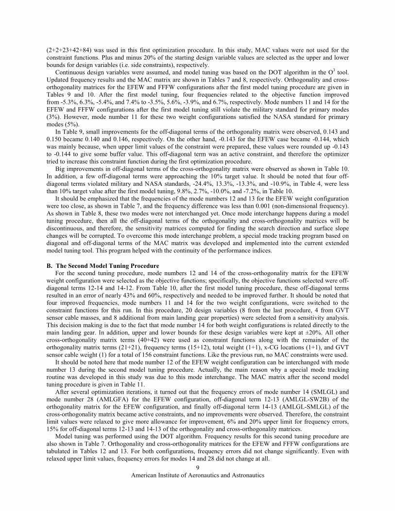
Big improvements in off-diagonal terms of the cross-orthogonality matrix were observed as shown in Table 10.In addition, a few off-diagonal terms were approaching the 10% target value. It should be noted that four off-diagonal terms violated military and NASA standards, -24.4%, 13.3%, -13.3%, and -10.9%, in Table 4, were less than 10% target value after the first model tuning, 9.8%, 2.7%, -10.0%, and -7.2%, in Table 10.
It should be emphasized that the frequencies of the mode numbers 12 and 13 for the EFEW weight configuration were too close, as shown in Table 7, and the frequency difference was less than 0.001 (non-dimensional frequency).As shown in Table 8, these two modes were not interchanged yet. Once mode interchange happens during a model tuning procedure, then all the off-diagonal terms of the orthogonality and cross-orthogonality matrices will be discontinuous, and therefore, the sensitivity matrices computed for finding the search direction and surface slope changes will be corrupted. To overcome this mode interchange problem, a special mode tracking program based on diagonal and off-diagonal terms of the MAC matrix was developed and implemented into the current extended model tuning tool. This program helped with the continuity of the performance indices.
B. The Second Model Tuning ProcedureFor the second tuning procedure, mode numbers 12 and 14 of the cross-orthogonality matrix for the EFEW
weight configuration were selected as the objective functions; specifically, the objective functions selected were off-diagonal terms 12-14 and 14-12. From Table 10, after the first model tuning procedure, these off-diagonal terms resulted in an error of nearly 43% and 60%, respectively and needed to be improved further. It should be noted thatfour improved frequencies, mode numbers 11 and 14 for the two weight configurations, were switched to the constraint functions for this run. In this procedure, 20 design variables (8 from the last procedure, 4 from GVT sensor cable masses, and 8 additional from main landing gear properties) were selected from a sensitivity analysis.This decision making is due to the fact that mode number 14 for both weight configurations is related directly to the main landing gear. In addition, upper and lower bounds for these design variables were kept at ±20%. All other cross-orthogonality matrix terms (40+42) were used as constraint functions along with the remainder of the orthogonality matrix terms (21+21), frequency terms (15+12), total weight (1+1), x-CG locations (1+1), and GVT sensor cable weight (1) for a total of 156 constraint functions. Like the previous run, no MAC constraints were used.
It should be noted here that mode number 12 of the EFEW weight configuration can be interchanged with mode number 13 during the second model tuning procedure. Actually, the main reason why a special mode tracking routine was developed in this study was due to this mode interchange. The MAC matrix after the second model tuning procedure is given in Table 11.
After several optimization iterations, it turned out that the frequency errors of mode number 14 (SMLGL) and mode number 28 (AMLGFA) for the EFEW configuration, off-diagonal term 12-13 (AMLGL-SW2B) of the orthogonality matrix for the EFEW configuration, and finally off-diagonal term 14-13 (AMLGL-SMLGL) of the cross-orthogonality matrix became active constraints, and no improvements were observed. Therefore, the constraint limit values were relaxed to give more allowance for improvement, 6% and 20% upper limit for frequency errors, 15% for off-diagonal terms 12-13 and 14-13 of the orthogonality and cross-orthogonality matrices.
Model tuning was performed using the DOT algorithm. Frequency results for this second tuning procedure are also shown in Table 7. Orthogonality and cross-orthogonality matrices for the EFEW and FFFW configurations are tabulated in Tables 12 and 13. For both configurations, frequency errors did not change significantly. Even with relaxed upper limit values, frequency errors for modes 14 and 28 did not change at all.
10American Institute of Aeronautics and Astronautics
Results for the orthogonality matrices for both weight configurations after the second procedure are shown in Table 12. Note for this procedure, all of the off-diagonal terms for the orthogonality matrices were selected as constraints, not objective functions. Similarly orthogonality matrices for both weight configurations were unchanged during the second optimization run. Off-diagonal term 12-13 was an active constraint, and this term didn’t become better nor worse even with relaxed upper limit value.
Results for the off-diagonal terms of the cross-orthogonality matrix after the second tuning procedure are shown in Table 13. In comparison to the first tuning procedure results in Table 10, some off-diagonal terms, mostly constraints, slightly improved for both configurations. However, the objective functions for this procedure were off-diagonal terms 12-14 and 14-12 for the EFEW configuration and have improved negligibly from -0.604 to -0.600 and from -0.434 to -0.433.
C. The Third Model Tuning ProcedureBased on the results from the second model tuning procedure, there was very minimal improvement in the cross-
orthogonality matrix as shown in Table 13, when compared to the first model tuning run in Table 10. The objective functions and corresponding design variables during the previous model tuning procedure were reviewed prior to conducting this third model tuning procedure. By looking at some of the previous designs, there was a possibility that a better design configuration existed. Just because the output of the previous procedure resulted in miniscule improvement does not imply that the O3 tool program did not find a better optimization configuration in one of its iterations. From the previous optimization history (POH), a better starting configuration was selected. This design configuration was not selected by the DOT since some of the performance indices had violated constraint functions,which were actually acceptable violations. The results from this selected configuration are displayed from Tables 14 through 17 for frequencies, the MAC matrix, the mass orthogonality matrix, and the cross-orthogonality matrix, respectively.
When comparing frequency results in Tables 7 and 14, it can be seen that there was a mode interchange between modes 12 and 13 for both weight configurations as the frequencies were switched. As shown in Tables 7 and 14,frequencies of mode number 14 for the EFEW and FFFW configurations after DOT-02 in Table 7, 5.6 % and 6.7%,were all less than 5% (even smaller than 3%) in Table 14 (under POH). Also, notice that the frequency for mode 28 of the EFEW weight configuration reached the constraint value limit of 20%. In Table 15, the MAC values for mode 14 of the EFEW and FFFW configurations based on the selected POH was 0.97 and 0.61, respectively; these MAC values are far better than the 0.55 and 0.39 from DOT-02 as shown in Table 11. In addition, the mass orthogonality matrices for both weight configurations improved as well, as shown in Table 16; however, for the EFEW, off-diagonal term 12-13 increased when compared to the second model tuning results, while off-diagonal term 12-14improved to 0.107 when compared to 0.140 in Table 12. For the FFFW, off-diagonal term 12-14 also significantly improved from 0.146 to 0.118.
Furthermore, Table 17 displays a drastic improvement in the cross-orthogonality matrices when compared to Table 13 after the second model tuning procedure. After the first model tuning procedure in Table 10, off-diagonal terms 12-13 and 13-12 for the EFEW configuration were constrained to be a maximum value of 10%. After the second model tuning procedure, in Table 13, these two off-diagonal terms satisfied the 10% requirement. Although these two off-diagonal terms in Table 17 violated the 10% requirement; however, compared to Table 13 results, the cross-orthogonality matrix in Table 17 had a more improved configuration when compared to the results in Table 13. Significant improvements were observed for the EFEW off-diagonal terms 12-14 and 14-12, which went from -0.433 to -0.153 and -0.600 to 0.000, respectively. Likewise, the FFFW off-diagonal terms 12-14 and 14-12 (14-13 due to mode interchange) improved magnitude-wise from 0.218 to 0.168 and from 0.362 to 0.296. On the other hand, some mode shape off-diagonal terms did worsen a bit; most significant was the EFEW off-diagonal term 12-13 (12-12 due to mode interchange), which was 0.032 after the second model tuning procedure, but was 0.250 based on POH. Overall, this POH configuration is much better than the results after the second model tuning procedure. By selecting an improved optimization configuration based on the POH as the new starting point for this run, the optimization results for this third model tuning procedure can be improved significantly.
Based on the cross-orthogonality matrix from the POH in Table 17, off-diagonal terms 12-12 (SW2B-AMLGL)of the EFEW configuration and 14-13 (SMLGL-SW2B) of the FFFW configuration were selected as the objective functions for this third model tuning procedure. Same design variables were used like before, but with the addition of four main landing gear design variables for a total of 24 design variables. Constraint functions consisted of all other cross-orthogonality matrix terms (41+41), mass orthogonality matrix terms (21+21), frequency terms (15+12), total weight (1+1), x-CG locations (1+1), and GVT sensor cable weight (1) for a total of 156 constraint functions.Again, the DOT algorithm was used for this optimization procedure. For both weight configurations, constraint value limits of 15% were used for off-diagonal terms 12-13, 12-14, 13-12, and 14-12 of the orthogonality matrices

11American Institute of Aeronautics and Astronautics
and off-diagonal terms 12-12 (mode interchange), 12-14, 13-13 (mode interchange), and 14-13 of the cross-orthogonality matrices. For all other off-diagonal terms, 10% limit values were used.
Table 14 also shows the frequency results for the third model tuning procedure. The MAC matrix after the third model tuning procedure is displayed in Table 18. MAC terms for mode number 14 improved for both weight configurations. Mass orthogonality matrix results are shown in Table 19. Small improvements were observed for the EFEW configuration with the off-diagonal term 12-13 going from -0.150 to -0.142 and the off-diagonal term 12-14reducing from 0.107 to 0.091. Similarly, the off-diagonal term for the FFFW configuration went from 0.118 to 0.105. Cross-orthogonality matrix results are shown in Table 20. Both objective function terms improved with the EFEW mode interchanged off-diagonal term 12-12 improving the most from an initial value of 0.250 to 0.179, whereas the FFFW mode interchanged off-diagonal term 14-13 improving slightly from 0.296 to 0.292.
D. The Fourth Model Tuning ProcedureBased on frequency results after the third model tuning procedure in Table 14, the frequency result for mode
number 28 of the EFEW configuration stood out due to the fact that frequency error was allowed to be at the maximum value of 20%. For this model tuning procedure, the goal was to improve this particular secondary mode frequency and as a result, frequency of the EFEW mode number 28 was selected as the objective function for this run. Similar to the last procedure, identical design variables were used with constraint functions consisting of all other cross-orthogonality matrix terms (42+42), mass orthogonality matrix terms (21+21), frequency terms (14+12), total weight (1+1), x-CG locations (1+1), and GVT sensor cable weight (1) for a total of 157 constraint functions.The DOT algorithm was also used again for this optimization procedure.
Frequency results for the fourth model tuning procedure are tabulated in Table 14. Notice that the frequency for the EFEW mode number 28, which was the objective function for this run, improved from -20% from the previous procedure to -16.7%. MAC results for this procedure are shown in Table 21; a slight improvement was observed for the FFFW weight configuration where mode number 14 went from 0.69 in the last procedure to 0.70 for this run.Table 22 shows the results of the mass orthogonality matrix; only a slight improvement was seen for the off-diagonal term 12-13 for the EFEW configuration. Off-diagonal term 12-14 for the EFEW and FFFW increased from 0.091 to 0.110 and from 0.105 to 0.120, respectively. Cross-orthogonality matrix results are displayed in Table 23. Not much change was observed between the last run and this run, with the exception of the off-diagonal term 12-14 for the FFFW weight configuration which went from a magnitude of 0.153 to 0.143.
The design variable changes of the model tuning procedures are summarized in Table 24, which actually displays the design variable percentage changes between each model tuning procedure. Notice that the percentage change for many of the main landing gear design variables after the fourth model tuning procedure (DOT-04) approached the ±20% side constraint limit. In addition, the smallest MAC value, largest frequency error, largest off-diagonal terms of orthogonality as well as the cross-orthogonality matrices were all related to the main landing gear. Therefore, it can be concluded that the FE model pertaining to the main landing gear was not accurate enough in order to allow significant change or improvement. It was later found that there was an idealization error with the main landing gear. This reasoning for this idealization error is presented in Fig. 16. In Fig. 16, the main landing-gear was originally designed as tapered and curved beam types of structure. When creating the FE model, the tapered and curved regions of the main landing gear was modeled as uniform and straight beams, as opposed to tapered and curved beams, respectively. It was so difficult to improve properties related to the main landing gear since only a single uniform sectional property was used for the whole tapered region.
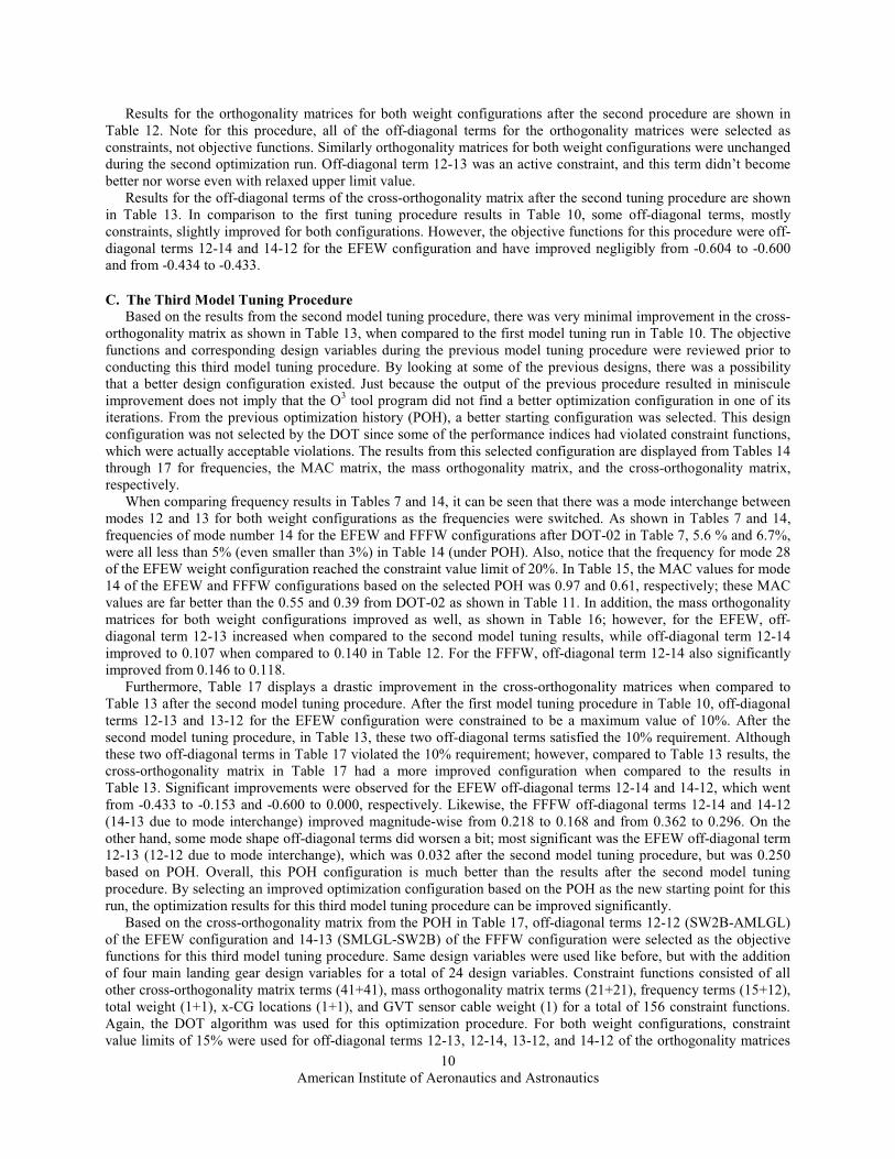
Non-dimensional flutter speeds and frequencies after the fourth model tuning are summarized in Table 5.Corresponding speed versus damping, V-g, and speed versus frequency, V-f, curves of this model with the EFEW configuration at a Mach number of 0.160 from the matched flutter analyses are given in Fig. 17. Improved frequencies and mode shapes in this study increased average flutter speeds by 7.6% compared to the baseline model.
VI. ConclusionFor the X-56A flight-test support, NASA AFRC has undertaken the task of improving the GVT test-validated
structural dynamic finite element model. Using an in-house O3 tool developed by NASA AFRC’s structural dynamics group, along with the Nastran program, structural model tuning is being conducted so as to improve the correlation between numerical and experimental modal data in order to reduce model uncertainties by meeting specified NASA and military standards.
Structural dynamic model tuning of the aircraft was performed in stages, starting with tuning of the frequency, followed by the cross-orthogonality (mode shape) matrix. A total of four structural dynamic model tuning runs were conducted focusing on the improvement in frequency errors and the off-diagonal terms of the cross-orthogonality
12American Institute of Aeronautics and Astronautics
matrices for both the EFEW and the FFFW configurations of the X-56A aircraft in a single optimization run. Other properties such as weight of GVT sensor cables, total weight, CG location, and off-diagonal terms of the orthogonality matrix were primarily used as constraints as the current configurations met the majority of the defined criteria. MAC constraints were not used as objective or constraint functions. However, the MAC values were used in a mode tracking program to overcome mode interchange problems during model tuning procedure.
The first and second model tuning procedures focused on the improvement of frequencies and off-diagonal terms of the cross-orthogonality matrices in order to meet the NASA standard by using main landing gear, Young’s modulus, and Shear modulus design variables. All of the off-diagonal terms violate military and NASA standards,which were subsequently improved after the first two model tuning procedures. An average of 3.8% of improvement was observed in the cross-orthogonality matrices. Slight violation of target frequency values was also observed after the first two model tuning procedures.
Before the third and fourth model tuning procedures, previous optimization histories were reviewed and a much better design configuration was found by change. By selecting an improved optimization configuration based on POH as the new starting point, the optimization results for the third and fourth model tuning procedures were improved significantly. It should be noted that the largest correlation errors were mostly associated with the main landing gear due to the existence of the idealization error related to the main landing gear.
Finally, it should be emphasized that the performance indices based on each individual element of frequency errors and the off-diagonal terms of the orthogonality and cross-orthogonality matrices introduced in this study wereeasier to use than the norm average based model tuning method.2,4 In the case of the norm based approach, the total number of performance indices was a lot smaller than the current method; however, it was not easy to control each individual off-diagonal term when compared to the current approach.
AcknowledgmentsThe work presented in this paper was funded by the Aero Science Project under the ARMD Fundamental
Aeronautics Program. The project managers at NASA AFRC were Mark Davis and Robert Navarro. The authors also thank Jeff Beranek at Lockheed Martin Skunk Works (Palmdale, California) for his support in providing the finite element models and the ground vibration test data during this research. Finally, thanks to Pete Flick at the Air Force Research Laboratory for providing the flight hardware and test data to NASA.

13American Institute of Aeronautics and Astronautics
Tables
Table 1. The measured and computed flexible modes of the X-56A aircraft.
EFEW configurationGVT data Nastran results
Target error (%)Mode
numberMode shape Frequency
Final design Baseline
Frequency Error (%) Mode number Frequency Error (%)
7 SW1B 1.067 1.035 -3.0 7 1.090 2.1 58 AW1B 1.543 1.534 -0.5 8 1.540 -0.2 59 SW1T 3.223 2.781 -13.7 9 3.159 -2.0 511 AW1T 3.839 3.522 -8.3 11 3.636 -5.3 512 SW2B 4.440 4.127 -7.1 12 4.514 1.7 513 AMLGL 4.466 4.262 -4.6 13 4.567 2.3 514 SMLGL 4.666 4.467 -4.3 14 4.961 6.3 515 BoomH 5.273 4.530 -14.1 15 5.223 -0.9 1018 AW2B 6.026 5.404 -10.3 18 6.061 0.6 1019 SWL 6.264 5.815 -7.2 19 6.189 -1.2 1025 SW3B 9.346 9.798 4.8 25 9.416 0.8 1026 AW3B 10.598 9.889 -6.7 27 11.048 4.2 1028 AMLGFA 11.930 10.969 -8.1 26 10.035 -15.9 1030 AW2T 12.405 11.986 -3.4 30 12.811 3.3 10
Total weight 366.7 366.0 -0.18 5x-CG location 165.0 164.7 -0.16 5y-CG location -0.1 0.3 -413.z-CG location N/A 101.9 N/A
FFFW configurationGVT data Nastran results
Target error (%)Mode
numberMode shape Frequency
Final design Baseline
Frequency Error (%) Mode number Frequency Error (%)
7 SW1B 1.000 0.937 -6.3 7 1.001 0.1 58 AW1B 1.411 1.392 -1.3 8 1.398 -0.9 59 SW1T 2.938 2.608 -11.2 9 2.912 -0.9 511 AW1T 3.651 2.932 -19.7 11 3.454 -5.4 512 SW2B 4.346 3.898 -10.3 12 4.285 -1.4 513 AMLGL 4.408 5.393 22.4 13 4.446 0.9 514 SMLGL 4.601 4.159 -9.6 14 4.944 7.4 516 BoomH 5.276 4.476 -15.2 16 5.217 -1.1 1019 SWL 6.144 5.251 -14.5 19 6.018 -2.0 1024 SW3B 8.657 8.161 -5.7 24 8.673 0.2 1025 NLGFA 9.129 9.816 7.5 25 9.186 0.6 1028 AW2T 11.540 10.076 -12.7 30 11.704 1.4 10
Total weight 488.9 489.1 0.04 5x-CG location 165.2 165.3 0.04 5y-CG location 0.4 0.2 -41.5z-CG location N/A 101.4 N/A

14American Institute of Aeronautics and Astronautics
Table 2. MAC matrix of the X-56A baseline model.
EFEW configurationMode shape SW1B AW1B SW1T AW1T SW2B AMLGL SMLGL
Mode shape Mode number 7* 8 9 11 12 13 14SW1B 7** 0.99 0.00 0.00 0.00 0.08 0.00 0.01AW1B 8 0.00 1.00 0.00 0.00 0.00 0.09 0.00SW1T 9 0.01 0.00 0.91 0.00 0.01 0.00 0.01AW1T 11 0.00 0.01 0.00 0.97 0.00 0.16 0.00SW2B 12 0.09 0.00 0.09 0.01 0.95 0.02 0.27
AMLGL 13 0.00 0.06 0.00 0.43 0.03 0.93 0.02SMLGL 14 0.05 0.00 0.07 0.00 0.93 0.00 0.51
FFFW configurationMode shape SW1B AW1B SW1T AW1T SW2B AMLGL SMLGL
Mode shape Mode number 7* 8 9 11 12 13 14SW1B 7** 0.99 0.00 0.02 0.00 0.08 0.00 0.01AW1B 8 0.00 1.00 0.00 0.01 0.00 0.07 0.00SW1T 9 0.04 0.00 0.93 0.00 0.01 0.00 0.02AW1T 11 0.00 0.04 0.00 0.90 0.01 0.09 0.01SW2B 12 0.07 0.00 0.06 0.00 0.99 0.00 0.14
AMLGL 13 0.00 0.04 0.00 0.37 0.01 0.96 0.01SMLGL 14 0.03 0.00 0.04 0.00 0.84 0.02 0.38
*: Nastran mode number**: GVT mode number
Table 3. Orthogonality matrix of the X-56A baseline model with respect to GVT modes.
EFEW configurationMode shape SW1B AW1B SW1T AW1T SW2B AMLGL SMLGL
Mode shape Mode number 7** 8 9 11 12 13 14SW1B 7** 1.000 -0.021 -0.054 -0.011 0.026 0.024 -0.033AW1B 8 -0.021 1.000 0.012 0.002 0.004 0.040 0.002SW1T 9 -0.054 0.012 1.000 0.004 0.035 -0.007 -0.025AW1T 11 -0.011 0.002 0.004 1.000 0.022 -0.093 0.003SW2B 12 0.026 0.004 0.035 0.022 1.000 -0.143 0.143
AMLGL 13 0.024 0.040 -0.007 -0.093 -0.143 1.000 0.006SMLGL 14 -0.033 0.002 -0.025 0.003 0.143 0.006 1.000
FFFW configurationMode shape SW1B AW1B SW1T AW1T SW2B AMLGL SMLGL
Mode shape Mode number 7** 8 9 11 12 13 14SW1B 7** 1.000 0.013 -0.048 0.014 0.019 0.008 -0.066AW1B 8 0.013 1.000 -0.010 0.013 -0.005 -0.062 -0.011SW1T 9 -0.048 -0.010 1.000 -0.019 0.007 -0.013 -0.028AW1T 11 0.014 0.013 -0.019 1.000 -0.026 0.093 0.017SW2B 12 0.019 -0.005 0.007 -0.026 1.000 0.003 0.150
AMLGL 13 0.008 -0.062 -0.013 0.093 0.003 1.000 -0.077SMLGL 14 -0.066 -0.011 -0.028 0.017 0.150 -0.077 1.000
**: GVT mode number
15American Institute of Aeronautics and Astronautics
Table 4. Cross-orthogonality matrix of the X-56A baseline model with respect to GVT modes (check mode shapes).
EFEW configurationMode shape SW1B AW1B SW1T AW1T SW2B AMLGL SMLGL
Mode shape Mode number 7* 8 9 11 12 13 14SW1B 7** -1.000 -0.015 -0.032 0.006 0.026 0.012 -0.074AW1B 8 0.005 1.000 0.004 0.015 0.005 0.031 0.003SW1T 9 0.028 0.007 1.000 -0.021 -0.151 -0.004 -0.024AW1T 11 0.000 0.016 0.003 -1.000 0.010 0.095 -0.002SW2B 12 0.000 0.005 0.162 -0.026 1.000 -0.244 -0.451
AMLGL 13 -0.009 0.013 0.020 0.211 0.133 1.000 -0.004SMLGL 14 -0.011 0.003 0.098 0.006 0.618 -0.076 1.000
FFFW configurationMode shape SW1B AW1B SW1T AW1T SW2B AMLGL SMLGL
Mode shape Mode number 7* 8 9 11 12 13 14SW1B 7** 1.000 -0.007 0.032 0.009 0.033 0.011 0.064AW1B 8 0.003 -1.000 0.008 0.003 -0.004 -0.056 0.012SW1T 9 -0.023 0.004 -1.000 -0.018 -0.133 -0.005 0.016AW1T 11 -0.018 -0.004 0.029 1.000 0.014 -0.109 -0.009SW2B 12 -0.010 0.003 -0.132 -0.003 1.000 -0.052 0.220
AMLGL 13 -0.003 0.008 -0.004 0.208 0.070 1.000 0.003SMLGL 14 -0.013 0.011 -0.049 0.012 0.366 -0.121 -1.000
*: Nastran mode number**: GVT mode number
Table 5. Non-dimensional flutter speeds and frequencies of the X-56A models with EFEW at Mach = 0.16.
Non-dimensional flutter speed
Flutter mode Final design Baseline After fourth tuningSpeed Difference* (%) Speed Difference+ (%)
First 0.981 1.135 15.7 1.190 21.3Second 1.090 1.462 34.1 1.580 44.9Third 1.161 1.809 55.8 1.883 62.2
Non-dimensional flutter frequency
Flutter mode Final design Baseline After fourth tuningFrequency Difference* (%) Frequency Difference+ (%)
First 0.653 0.663 1.6 0.664 1.7Second 2.014 2.415 19.9 2.527 25.5Third 1.390 2.509 80.5 2.755 98.2
*: difference = (baseline-final design)/ final design+: difference = (after tuning-final design)/ final design

16A
mer
ican
Inst
itute
of A
eron
autic
s and
Ast
rona
utic
s
Tab
le 6
. Mod
al p
artic
ipat
ion
fact
ors (
%) o
f the
X-5
6Aai
rcra
ft (1
st:f
irst
flut
ter
mod
e; 2
nd:s
econ
d flu
tter
mod
e; 3
rd:t
hird
flut
ter
mod
e).
EFEW
con
figur
atio
n
GV
T m
ode
num
ber
Mod
e sh
ape
Fina
l des
ign
Bas
elin
e m
odel
M=
0.13
0M
=0.
195
M=
0.28
4M
=0.
130
M=
0.19
5M
=0.
284
1st
2nd
3rd
1st
2nd
3rd
1st
2nd
3rd
1st
2nd
3rd
1st
2nd
3rd
1st
2nd
3rd
Primary modes
1-6
Rig
id31
.630
.740
.327
.532
.633
.025
.034
.325
.233
.733
.342
.827
.935
.740
.524
.639
.040
.27
SW1B
15.0
9.5
0.0
12.1
8.8
0.0
9.7
8.1
0.0
17.0
10.0
0.0
14.9
9.2
0.0
13.0
8.6
0.0
8A
W1B
0.0
0.0
27.3
0.0
0.0
31.1
0.0
0.0
35.1
0.0
0.0
8.3
0.0
0.0
12.5
0.0
0.0
28.1
9SW
1T44
.354
.60.
051
.154
.40.
056
.154
.10.
038
.643
.00.
047
.841
.50.
053
.739
.70.
011
AW
1T0.
00.
027
.30.
00.
031
.10.
00.
035
.11.
92.
80.
01.
82.
50.
01.
72.
20.
012
SW2B
0.0
0.0
0.1
0.0
0.0
0.0
0.0
0.0
0.0
0.0
0.0
42.1
0.0
0.0
40.9
0.0
0.0
28.1
13A
MLG
L1.
51.
30.
01.
30.
90.
01.
20.
70.
00.
00.
04.
50.
00.
04.
20.
00.
02.
514
SMLG
L1.
30.
70.
01.
20.
60.
01.
20.
60.
02.
67.
10.
01.
77.
60.
01.
27.
50.
0T
otal
93.7
96.8
95.0
93.2
97.3
95.2
93.2
97.8
95.4
93.8
96.2
97.7
94.1
96.5
98.1
94.2
97.0
98.9
Secondary modes
15B
oom
H0.
00.
00.
10.
00.
00.
00.
00.
00.
00.
71.
60.
00.
71.
70.
00.
61.
70.
026
AM
LGFA
0.0
0.0
1.6
0.0
0.0
1.6
0.0
0.0
1.7
0.0
0.0
0.4
0.0
0.0
0.4
0.0
0.0
0.4
28SW
2T2.
91.
10.
03.
10.
90.
03.
20.
80.
02.
61.
00.
02.
50.
80.
02.
50.
60.
030
AW
2T0.
00.
01.
60.
00.
01.
90.
00.
01.
91.
80.
50.
01.
70.
40.
01.
70.
30.
0T
otal
2.9
1.1
3.3
3.1
0.9
3.5
3.2
0.8
3.6
4.1
3.1
1.4
4.9
2.9
0.4
4.8
2.6
0.4
FFFW
con
figur
atio
n
GV
T m
ode
num
ber
Mod
e sh
ape
Fina
l des
ign
Bas
elin
e m
odel
M=
0.13
0M
=0.
195
M=
0.28
4M
=0.
130
M=
0.19
5M
=0.
284
1st
2nd
3rd
1st
2nd
3rd
1st
2nd
3rd
1st
2nd
3rd
1st
2nd
3rd
1st
2nd
3rd
Primary modes
1-6
Rig
id42
.432
.344
.738
.536
.238
.434
.840
.539
.042
.129
.235
.336
.832
.034
.432
.636
.032
.47
SW1B
12.9
11.5
0.0
11.8
10.9
0.0
11.1
10.3
0.0
14.9
10.4
0.0
12.8
9.5
0.0
10.7
8.9
0.0
8A
W1B
0.0
0.0
5.2
0.0
0.0
27.2
0.0
0.0
25.0
0.0
0.0
1.6
0.0
0.0
1.3
0.0
0.0
1.2
9SW
1T38
.046
.30.
042
.042
.90.
045
.939
.50.
029
.737
.10.
035
.434
.10.
040
.630
.80.
011
AW
1T0.
00.
044
.00.
00.
027
.20.
00.
025
.00.
70.
80.
00.
70.
70.
00.
80.
70.
012
SW2B
0.1
0.1
0.0
0.1
0.1
0.0
0.1
0.1
0.0
0.0
0.0
50.2
0.0
0.0
50.1
0.0
0.0
50.7
13A
MLG
L0.
00.
02.
50.
00.
01.
30.
00.
01.
47.
620
.30.
08.
221
.90.
08.
622
.20.
014
SMLG
L1.
96.
80.
01.
67.
40.
01.
37.
50.
00.
00.
07.
30.
00.
08.
40.
00.
09.
5T
otal
95.3
97.0
96.4
94.0
97.5
94.1
93.2
97.9
90.4
95.0
97.8
94.4
93.9
98.2
94.2
93.3
98.6
93.8
Secondary modes
16B
oom
H0.
00.
01.
10.
00.
01.
20.
00.
01.
40.
00.
01.
80.
00.
01.
90.
00.
02.
119
SWL
0.5
0.7
0.0
0.7
0.6
0.0
0.8
0.5
0.0
0.0
0.0
2.3
0.0
0.0
2.3
0.0
0.0
2.4
24SW
3B1.
30.
50.
01.
60.
50.
01.
90.
50.
00.
00.
00.
00.
00.
00.
00.
00.
00.
025
NLG
FA2.
00.
90.
02.
50.
70.
02.
90.
60.
03.
11.
20.
03.
80.
90.
04.
30.
80.
030
AW
2T0.
00.
01.
10.
00.
03.
00.
00.
05.
60.
90.
20.
01.
10.
20.
01.
20.
20.
0T
otal
3.8
2.1
2.2
4.8
1.8
4.2
5.6
1.6
7.0
4.0
1.4
4.1
4.9
1.1
4.2
5.5
1.0
4.5

17American Institute of Aeronautics and Astronautics
Table 7. Flexible modes of the X-56A aircraft after the first and second model tuning procedures.
EFEW configurationGVT data Nastran results
Target error (%)Mode
numberMode shape
DOT-01 DOT-02Mode
number Frequency Error (%) Mode number Frequency Error (%)
7 SW1B 7 1.086 1.7 7 1.086 1.7 58 AW1B 8 1.535 -0.5 8 1.535 -0.5 59 SW1T 9 3.193 -0.9 9 3.193 -0.9 511 AW1T 11 3.703 -3.5 11 3.703 -3.5 512 SW2B 12 4.553 2.5 12 4.553 2.5 513 AMLGL 13 4.554 2.0 13 4.554 2.0 514 SMLGL 14 4.927 5.6 14 4.927 5.6 615 BoomH 15 5.223 -0.9 15 5.223 -0.9 1018 AW2B 18 6.064 0.6 18 6.065 0.6 1019 SWL 19 6.197 -1.1 19 6.197 -1.1 1025 SW3B 25 9.413 0.7 25 9.414 0.7 1026 AW3B 27 11.042 4.2 27 11.042 4.2 1028 AMLGFA 26 10.009 -16.1 26 10.009 -16.1 2030 AW2T 30 12.894 3.9 30 12.894 3.9 10
Total weight 366.0 -0.18 366.0 -0.18 5x-CG location 164.7 -0.16 164.7 -0.16 5y-CG location 0.3 -413. 0.3 -413.z-CG location 101.9 101.9
FFFW configurationGVT data Nastran results
Target error (%)Mode
numberMode shape
DOT-01 DOT-02Mode
number Frequency Error (%) Mode number Frequency Error (%)
7 SW1B 7 0.997 -0.3 7 0.997 -0.3 58 AW1B 8 1.394 -1.2 8 1.394 -1.2 59 SW1T 9 2.935 -0.1 9 2.935 -0.1 511 AW1T 11 3.509 -3.9 11 3.510 -3.9 512 SW2B 12 4.336 -0.2 12 4.336 -0.2 513 AMLGL 13 4.446 0.9 13 4.446 0.9 514 SMLGL 14 4.909 6.7 14 4.909 6.7 6.716 BoomH 16 5.217 -1.1 16 5.217 -1.1 1019 SWL 19 6.023 -2.0 19 6.023 -2.0 1024 SW3B 24 8.674 0.2 24 8.674 0.2 1025 NLGFA 25 9.186 0.6 25 9.186 0.6 1028 AW2T 30 11.776 2.0 30 11.776 2.0 10
Total weight 489.1 0.05 489.1 0.05 5x-CG location 165.3 0.04 165.3 0.04 5y-CG location 0.2 -41.5 0.2 -41.5z-CG location 101.4 N/A 101.4 N/A

18American Institute of Aeronautics and Astronautics
Table 8. MAC matrix of the X-56A aircraft after the first model tuning procedure (DOT-01).
EFEW configurationMode shape SW1B AW1B SW1T AW1T SW2B AMLGL SMLGL
Mode shape Mode number 7* 8 9 11 12 13 14SW1B 7** 0.99 0.00 0.00 0.00 0.08 0.00 0.01AW1B 8 0.00 1.00 0.00 0.00 0.00 0.09 0.00SW1T 9 0.01 0.00 0.92 0.00 0.00 0.00 0.01AW1T 11 0.00 0.01 0.00 0.98 0.01 0.17 0.00SW2B 12 0.09 0.00 0.07 0.01 0.98 0.00 0.30
AMLGL 13 0.00 0.06 0.00 0.41 0.00 0.97 0.02SMLGL 14 0.05 0.00 0.06 0.00 0.92 0.03 0.55
FFFW configurationMode shape SW1B AW1B SW1T AW1T SW2B AMLGL SMLGL
Mode shape Mode number 7* 8 9 11 12 13 14SW1B 7** 0.99 0.00 0.02 0.00 0.08 0.00 0.01AW1B 8 0.00 1.00 0.00 0.02 0.00 0.07 0.00SW1T 9 0.04 0.00 0.95 0.00 0.00 0.00 0.02AW1T 11 0.00 0.04 0.00 0.93 0.01 0.10 0.01SW2B 12 0.07 0.00 0.04 0.00 0.99 0.00 0.15
AMLGL 13 0.00 0.04 0.00 0.33 0.01 0.97 0.01SMLGL 14 0.03 0.00 0.03 0.00 0.85 0.02 0.38
*: Nastran mode number**: GVT mode number
Table 9. Orthogonality matrix of the X-56A aircraft after the first model tuning procedure (DOT-01).
EFEW configurationMode shape SW1B AW1B SW1T AW1T SW2B AMLGL SMLGL
Mode shape Mode number 7** 8 9 11 12 13 14SW1B 7** 1.000 -0.021 -0.053 -0.011 0.026 0.024 -0.033AW1B 8 -0.021 1.000 0.012 0.002 0.004 0.039 0.002SW1T 9 -0.053 0.012 1.000 0.004 0.035 -0.007 -0.025AW1T 11 -0.011 0.002 0.004 1.000 0.021 -0.091 0.003SW2B 12 0.026 0.004 0.035 0.021 1.000 -0.144 0.140
AMLGL 13 0.024 0.039 -0.007 -0.091 -0.144 1.000 0.005SMLGL 14 -0.033 0.002 -0.025 0.003 0.140 0.005 1.000
FFFW configurationMode shape SW1B AW1B SW1T AW1T SW2B AMLGL SMLGL
Mode shape Mode number 7** 8 9 11 12 13 14SW1B 7** 1.000 0.013 -0.047 0.014 0.019 0.008 -0.065AW1B 8 0.013 1.000 -0.010 0.013 -0.005 -0.062 -0.011SW1T 9 -0.047 -0.010 1.000 -0.019 0.007 -0.013 -0.026AW1T 11 0.014 0.013 -0.019 1.000 -0.026 0.092 0.017SW2B 12 0.019 -0.005 0.007 -0.026 1.000 0.003 0.146
AMLGL 13 0.008 -0.062 -0.013 0.092 0.003 1.000 -0.076SMLGL 14 -0.065 -0.011 -0.026 0.017 0.146 -0.076 1.000
**: GVT mode number

19American Institute of Aeronautics and Astronautics
Table 10. Cross-orthogonality matrix of the X-56A aircraft after the first model tuning procedure (DOT-01).
EFEW configurationMode shape SW1B AW1B SW1T AW1T SW2B AMLGL SMLGL
Mode shape Mode number 7* 8 9 11 12 13 14SW1B 7** 1.000 0.015 0.033 0.007 -0.023 -0.015 -0.074AW1B 8 -0.006 -1.000 -0.004 0.008 0.000 -0.030 0.003SW1T 9 -0.027 -0.007 -1.000 -0.019 0.110 0.021 -0.024AW1T 11 0.000 -0.010 -0.003 -1.000 0.001 -0.064 -0.002SW2B 12 0.000 -0.004 -0.131 -0.020 -1.000 0.098 -0.434
AMLGL 13 0.010 -0.015 -0.016 0.178 0.027 -1.000 -0.003SMLGL 14 0.012 -0.003 -0.080 0.007 -0.604 -0.011 1.000
FFFW configurationMode shape SW1B AW1B SW1T AW1T SW2B AMLGL SMLGL
Mode shape Mode number 7* 8 9 11 12 13 14SW1B 7** -1.000 -0.007 -0.033 0.011 0.031 0.011 0.064AW1B 8 -0.003 -1.000 -0.007 0.010 -0.004 -0.055 0.012SW1T 9 0.023 0.004 1.000 -0.015 -0.100 -0.006 0.016AW1T 11 0.018 0.000 -0.028 1.000 0.013 -0.072 -0.009SW2B 12 0.009 0.003 0.103 -0.004 1.000 -0.051 0.218
AMLGL 13 0.003 0.009 0.002 0.170 0.069 1.000 0.002SMLGL 14 0.012 0.011 0.038 0.015 0.362 -0.121 -1.000
*: Nastran mode number**: GVT mode number
Table 11. MAC matrix of the X-56A aircraft after the second model tuning procedure (DOT-02).
EFEW configurationMode shape SW1B AW1B SW1T AW1T SW2B AMLGL SMLGL
Mode shape Mode number 7* 8 9 11 12 13 14SW1B 7** 0.99 0.00 0.00 0.00 0.08 0.01 0.01AW1B 8 0.00 1.00 0.00 0.00 0.00 0.08 0.00SW1T 9 0.01 0.00 0.92 0.00 0.00 0.00 0.01AW1T 11 0.00 0.01 0.00 0.98 0.02 0.16 0.00SW2B 12 0.09 0.00 0.07 0.01 0.98 0.01 0.30
AMLGL 13 0.00 0.06 0.00 0.41 0.00 0.95 0.02SMLGL 14 0.05 0.00 0.06 0.00 0.91 0.07 0.55
FFFW configurationMode shape SW1B AW1B SW1T AW1T SW2B AMLGL SMLGL
Mode shape Mode number 7* 8 9 11 12 13 14SW1B 7** 0.99 0.00 0.02 0.00 0.08 0.00 0.01AW1B 8 0.00 1.00 0.00 0.02 0.00 0.07 0.00SW1T 9 0.04 0.00 0.95 0.00 0.00 0.00 0.02AW1T 11 0.00 0.04 0.00 0.93 0.01 0.10 0.01SW2B 12 0.07 0.00 0.04 0.00 0.99 0.00 0.15
AMLGL 13 0.00 0.04 0.00 0.33 0.01 0.97 0.01SMLGL 14 0.03 0.00 0.03 0.00 0.85 0.02 0.39
*: Nastran mode number**: GVT mode number

20American Institute of Aeronautics and Astronautics
Table 12. Orthogonality matrix of the X-56A aircraft after the second model tuning procedure (DOT-02).
EFEW configurationMode shape SW1B AW1B SW1T AW1T SW2B AMLGL SMLGL
Mode shape Mode number 7** 8 9 11 12 13 14SW1B 7** 1.000 -0.021 -0.053 -0.011 0.026 0.024 -0.033AW1B 8 -0.021 1.000 0.012 0.002 0.004 0.039 0.002SW1T 9 -0.053 0.012 1.000 0.004 0.035 -0.007 -0.025AW1T 11 -0.011 0.002 0.004 1.000 0.021 -0.091 0.003SW2B 12 0.026 0.004 0.035 0.021 1.000 -0.144 0.140
AMLGL 13 0.024 0.039 -0.007 -0.091 -0.144 1.000 0.005SMLGL 14 -0.033 0.002 -0.025 0.003 0.140 0.005 1.000
FFFW configurationMode shape SW1B AW1B SW1T AW1T SW2B AMLGL SMLGL
Mode shape Mode number 7** 8 9 11 12 13 14SW1B 7** 1.000 0.013 -0.047 0.014 0.019 0.008 -0.065AW1B 8 0.013 1.000 -0.010 0.013 -0.005 -0.062 -0.011SW1T 9 -0.047 -0.010 1.000 -0.019 0.007 -0.013 -0.026AW1T 11 0.014 0.013 -0.019 1.000 -0.026 0.092 0.017SW2B 12 0.019 -0.005 0.007 -0.026 1.000 0.003 0.146
AMLGL 13 0.008 -0.062 -0.013 0.092 0.003 1.000 -0.076SMLGL 14 -0.065 -0.011 -0.026 0.017 0.146 -0.076 1.000
**: GVT mode number
Table 13. Cross-orthogonality matrix of the X-56A aircraft after the second model tuning procedure (DOT-02).
EFEW configurationMode shape SW1B AW1B SW1T AW1T SW2B AMLGL SMLGL
Mode shape Mode number 7* 8 9 11 12 13 14SW1B 7** -1.000 0.015 0.033 0.007 -0.022 -0.017 -0.074AW1B 8 0.006 -1.000 -0.004 0.008 0.002 -0.030 0.003SW1T 9 0.027 -0.007 -1.000 -0.019 0.108 0.028 -0.024AW1T 11 0.000 -0.010 -0.003 -1.000 0.005 -0.064 -0.002SW2B 12 0.000 -0.004 -0.131 -0.020 -1.000 0.032 -0.433
AMLGL 13 -0.010 -0.015 -0.016 0.179 0.100 -1.000 -0.003SMLGL 14 -0.012 -0.003 -0.080 0.007 -0.600 -0.051 1.000
FFFW configurationMode shape SW1B AW1B SW1T AW1T SW2B AMLGL SMLGL
Mode shape Mode number 7* 8 9 11 12 13 14SW1B 7** -1.000 0.007 -0.033 -0.011 0.031 0.011 0.064AW1B 8 -0.003 1.000 -0.007 -0.010 -0.004 -0.055 0.012SW1T 9 0.023 -0.004 1.000 0.015 -0.100 -0.006 0.016AW1T 11 0.018 0.000 -0.028 -1.000 0.013 -0.071 -0.009SW2B 12 0.009 -0.003 0.103 0.004 1.000 -0.051 0.218
AMLGL 13 0.003 -0.009 0.002 -0.170 0.069 1.000 0.002SMLGL 14 0.012 -0.011 0.039 -0.015 0.362 -0.121 -1.000
*: Nastran mode number**: GVT mode number

21American Institute of Aeronautics and Astronautics
Table 14. Flexible modes of the X-56A aircraft from previous history, and after the third and fourth model tuning procedures.
EFEW configurationGVT data Nastran results Target
errorMode Mode shape
POH DOT-03 DOT-04Mode Freq. Error* Mode Freq. Error Mode Freq. Error
7 SW1B 7 1.086 1.8 7 1.090 2.2 7 1.101 3.1 5(3)8 AW1B 8 1.543 0.0 8 1.549 0.4 8 1.565 1.5 5(3)9 SW1T 9 3.276 1.6 9 3.256 1.0 9 3.294 2.2 5(3)11 AW1T 11 3.823 -0.4 11 3.778 -1.6 11 3.834 -0.1 5(3)12 SW2B 13 4.642 4.6 13 4.611 3.9 13 4.662 5.0 513 AMLGL 12 4.415 -1.2 12 4.401 -1.5 12 4.460 -0.1 5(3)14 SMLGL 14 4.715 1.1 14 4.683 0.4 14 4.738 1.5 5(3)15 BoomH 15 5.217 -1.1 15 5.219 -1.0 15 5.222 -1.0 10(3)18 AW2B 18 6.106 1.3 18 6.105 1.3 18 6.149 2.0 10(3)19 SWL 19 6.242 -0.4 19 6.246 -0.3 19 6.270 0.1 10(3)25 SW3B 25 9.473 1.4 25 9.479 1.4 25 9.539 2.1 10(3)26 AW3B 27 11.01 3.9 27 11.22 -1.4 27 11.59 2.0 10(3)28 AMLGFA 26 9.544 -20.0 26 9.544 -20.0 26 9.938 -16.7 2030 AW2T 30 13.09 5.5 30 13.04 5.1 30 13.14 6.0 10
Total weight 368.1 0.37 367.7 0.28 367.4 0.20 5x-CG location 164.8 -0.14 164.8 -0.14 164.8 -0.15 5y-CG location 0.4 -481. 0.4 -466. 0.4 -462.z-CG location 101.7 N/A 101.8 N/A 101.8 N/A
FFFW configurationGVT data Nastran results Target
errorMode Mode shape
POH DOT-03 DOT-04Mode Freq. Error* Mode Freq. Error Mode Freq. Error
7 SW1B 7 0.999 -0.1 7 1.003 0.3 7 1.011 1.1 5(3)8 AW1B 8 1.402 -0.6 8 1.407 -0.2 8 1.421 0.8 5(3)9 SW1T 9 3.000 2.1 9 2.988 1.7 9 3.021 2.8 5(3)11 AW1T 11 3.615 -1.0 11 3.579 -2.0 11 3.630 -0.6 5(3)12 SW2B 13 4.469 2.8 13 4.427 1.9 13 4.481 3.1 5(3)13 AMLGL 12 4.357 -1.1 12 4.343 -1.5 12 4.401 -0.1 5(3)14 SMLGL 14 4.672 1.5 14 4.641 0.9 14 4.695 2.0 5(3)16 BoomH 16 5.219 -1.1 16 5.219 -1.1 16 5.220 -1.1 10(3)19 SWL 19 6.060 -1.4 19 6.068 -1.2 19 6.090 -0.9 10(3)24 SW3B 24 8.745 1.0 24 8.748 1.1 24 8.808 1.8 10(3)25 NLGFA 25 9.172 0.5 25 9.174 0.5 25 9.183 0.6 10(3)28 AW2T 30 11.93 3.4 30 11.88 3.0 30 11.96 3.6 10(5)
Total weight 491.1 0.46 490.8 0.39 490.5 0.33 5x-CG location 165.3 0.06 165.3 0.05 165.3 0.05 5y-CG location 0.3 -28.7 0.3 -31.5 0.3 -32.19z-CG Location 101.3 N/A 101.3 N/A 101.4 N/A
*: error in %

22American Institute of Aeronautics and Astronautics
Table 15. MAC matrix of the X-56A aircraft from previous history.
EFEW configurationMode shape SW1B AW1B SW1T AW1T SW2B AMLGL SMLGL
Mode shape Mode number 7* 8 9 11 13 12 14SW1B 7** 0.99 0.00 0.00 0.00 0.08 0.00 0.07AW1B 8 0.00 1.00 0.00 0.00 0.00 0.10 0.00SW1T 9 0.01 0.00 0.92 0.00 0.00 0.00 0.01AW1T 11 0.00 0.01 0.00 0.98 0.00 0.29 0.00SW2B 12 0.09 0.00 0.07 0.01 0.95 0.03 0.89
AMLGL 13 0.00 0.06 0.00 0.38 0.03 0.96 0.03SMLGL 14 0.05 0.00 0.06 0.00 0.88 0.00 0.97
FFFW configurationMode shape SW1B AW1B SW1T AW1T SW2B AMLGL SMLGL
Mode shape Mode number 7* 8 9 11 13 12 14SW1B 7** 0.99 0.00 0.02 0.00 0.08 0.00 0.03AW1B 8 0.00 1.00 0.00 0.02 0.00 0.07 0.00SW1T 9 0.04 0.00 0.95 0.00 0.00 0.00 0.02AW1T 11 0.00 0.04 0.00 0.93 0.01 0.16 0.01SW2B 12 0.07 0.00 0.04 0.00 0.99 0.00 0.34
AMLGL 13 0.00 0.04 0.00 0.31 0.01 0.97 0.01SMLGL 14 0.03 0.00 0.02 0.00 0.84 0.03 0.61
*: Nastran mode number**: GVT mode number
Table 16. Orthogonality matrix of the X-56A aircraft from previous history.
EFEW configurationMode shape SW1B AW1B SW1T AW1T SW2B AMLGL SMLGL
Mode shape Mode number 7** 8 9 11 12 13 14SW1B 7** 1.000 -0.022 -0.054 -0.011 0.030 0.025 -0.038AW1B 8 -0.022 1.000 0.013 0.000 0.007 0.034 0.002SW1T 9 -0.054 0.013 1.000 0.004 0.036 -0.009 -0.025AW1T 11 -0.011 0.000 0.004 1.000 0.020 -0.082 0.002SW2B 12 0.030 0.007 0.036 0.020 1.000 -0.150 0.107
AMLGL 13 0.025 0.034 -0.009 -0.082 -0.150 1.000 0.001SMLGL 14 -0.038 0.002 -0.025 0.002 0.107 0.001 1.000
FFFW configurationMode shape SW1B AW1B SW1T AW1T SW2B AMLGL SMLGL
Mode shape Mode number 7** 8 9 11 12 13 14SW1B 7** 1.000 0.014 -0.048 0.015 0.022 0.008 -0.069AW1B 8 0.014 1.000 -0.010 0.013 -0.006 -0.060 -0.011SW1T 9 -0.048 -0.010 1.000 -0.019 0.008 -0.015 -0.026AW1T 11 0.015 0.013 -0.019 1.000 -0.026 0.085 0.018SW2B 12 0.022 -0.006 0.008 -0.026 1.000 -0.002 0.118
AMLGL 13 0.008 -0.060 -0.015 0.085 -0.002 1.000 -0.076SMLGL 14 -0.069 -0.011 -0.026 0.018 0.118 -0.076 1.000
**: GVT mode number

23American Institute of Aeronautics and Astronautics
Table 17. Cross-orthogonality matrix of the X-56A aircraft from previous history.
EFEW configurationMode shape SW1B AW1B SW1T AW1T SW2B AMLGL SMLGL
Mode shape Mode number 7* 8 9 11 13 12 14SW1B 7** -1.000 0.015 -0.035 0.005 -0.063 -0.013 0.049AW1B 8 0.007 -1.000 0.004 0.002 -0.003 -0.038 -0.005SW1T 9 0.027 -0.008 1.000 -0.015 0.070 0.009 0.079AW1T 11 0.000 -0.005 0.008 -1.000 -0.006 0.030 -0.003SW2B 12 0.003 -0.008 0.121 0.001 -1.000 0.250 -0.153
AMLGL 13 -0.010 -0.003 0.014 0.097 -0.118 -1.000 -0.072SMLGL 14 -0.013 -0.004 0.074 0.013 0.000 0.083 -1.000
FFFW configurationMode shape SW1B AW1B SW1T AW1T SW2B AMLGL SMLGL
Mode shape Mode number 7* 8 9 11 13 12 14SW1B 7** -1.000 0.007 -0.034 0.010 0.037 0.008 -0.067AW1B 8 -0.004 1.000 -0.007 0.017 -0.006 -0.068 -0.012SW1T 9 0.023 -0.005 1.000 -0.012 -0.093 -0.007 -0.026AW1T 11 0.017 -0.004 -0.032 1.000 0.015 0.006 0.007SW2B 12 0.010 -0.004 0.096 -0.001 1.000 -0.094 -0.168
AMLGL 13 0.002 -0.002 0.001 0.117 0.106 1.000 0.005SMLGL 14 0.008 -0.012 0.041 0.023 0.296 -0.146 1.000
*: Nastran mode number**: GVT mode number
Table 18. MAC matrix of the X-56A aircraft after the third model tuning procedure (DOT-03).
EFEW configurationMode shape SW1B AW1B SW1T AW1T SW2B AMLGL SMLGL
Mode shape Mode number 7* 8 9 11 13 12 14SW1B 7** 0.99 0.00 0.00 0.00 0.08 0.00 0.07AW1B 8 0.00 1.00 0.00 0.01 0.00 0.09 0.00SW1T 9 0.01 0.00 0.93 0.00 0.00 0.00 0.00AW1T 11 0.00 0.01 0.00 0.99 0.01 0.31 0.01SW2B 12 0.09 0.00 0.06 0.01 0.97 0.01 0.89
AMLGL 13 0.00 0.07 0.00 0.34 0.02 0.98 0.03SMLGL 14 0.05 0.00 0.05 0.00 0.89 0.00 0.98
FFFW configurationMode shape SW1B AW1B SW1T AW1T SW2B AMLGL SMLGL
Mode shape Mode number 7* 8 9 11 13 12 14SW1B 7** 0.99 0.00 0.03 0.00 0.08 0.01 0.03AW1B 8 0.00 1.00 0.00 0.03 0.00 0.06 0.00SW1T 9 0.04 0.00 0.96 0.00 0.00 0.00 0.02AW1T 11 0.00 0.03 0.00 0.95 0.03 0.15 0.02SW2B 12 0.07 0.00 0.03 0.00 0.98 0.05 0.43
AMLGL 13 0.00 0.04 0.00 0.28 0.00 0.96 0.01SMLGL 14 0.03 0.00 0.02 0.00 0.86 0.01 0.69
*: Nastran mode number**: GVT mode number

24American Institute of Aeronautics and Astronautics
Table 19. Orthogonality matrix of the X-56A aircraft after the third model tuning procedure (DOT-03).
EFEW configurationMode shape SW1B AW1B SW1T AW1T SW2B AMLGL SMLGL
Mode shape Mode number 7** 8 9 11 12 13 14SW1B 7** 1.000 -0.016 -0.053 -0.006 0.035 0.022 -0.042AW1B 8 -0.016 1.000 0.005 -0.002 0.003 0.032 0.003SW1T 9 -0.053 0.005 1.000 -0.004 0.033 -0.001 -0.026AW1T 11 -0.006 -0.002 -0.004 1.000 0.007 -0.075 -0.002SW2B 12 0.035 0.003 0.033 0.007 1.000 -0.142 0.091
AMLGL 13 0.022 0.032 -0.001 -0.075 -0.142 1.000 0.005SMLGL 14 -0.042 0.003 -0.026 -0.002 0.091 0.005 1.000
FFFW configurationMode shape SW1B AW1B SW1T AW1T SW2B AMLGL SMLGL
Mode shape Mode number 7** 8 9 11 12 13 14SW1B 7** 1.000 0.008 -0.046 0.009 0.025 0.006 -0.071AW1B 8 0.008 1.000 -0.003 0.012 -0.001 -0.060 -0.011SW1T 9 -0.046 -0.003 1.000 -0.012 0.005 -0.008 -0.026AW1T 11 0.009 0.012 -0.012 1.000 -0.016 0.078 0.019SW2B 12 0.025 -0.001 0.005 -0.016 1.000 0.009 0.105
AMLGL 13 0.006 -0.060 -0.008 0.078 0.009 1.000 -0.072SMLGL 14 -0.071 -0.011 -0.026 0.019 0.105 -0.072 1.000
**: GVT mode number
Table 20. Cross-orthogonality matrix of the X-56A aircraft after the third model tuning procedure (DOT-03).
EFEW configurationMode shape SW1B AW1B SW1T AW1T SW2B AMLGL SMLGL
Mode shape Mode number 7* 8 9 11 13 12 14SW1B 7** 1.000 -0.016 -0.037 0.010 -0.065 -0.014 0.053AW1B 8 0.001 1.000 0.005 -0.005 0.001 -0.040 -0.003SW1T 9 -0.025 -0.002 1.000 -0.045 0.049 0.013 0.068AW1T 11 0.006 -0.001 -0.036 -1.000 -0.024 0.063 -0.017SW2B 12 -0.004 0.007 0.100 0.023 -1.000 0.179 -0.148
AMLGL 13 0.010 -0.002 0.024 0.051 -0.058 -1.000 -0.035SMLGL 14 0.015 0.003 0.065 0.023 0.009 0.038 -1.000
FFFW configurationMode shape SW1B AW1B SW1T AW1T SW2B AMLGL SMLGL
Mode shape Mode number 7* 8 9 11 13 12 14SW1B 7** -1.000 0.008 0.035 0.017 0.037 -0.016 -0.070AW1B 8 0.003 1.000 0.008 0.024 0.011 0.069 -0.011SW1T 9 0.021 0.005 -1.000 -0.032 -0.070 0.024 -0.028AW1T 11 0.023 -0.009 0.001 1.000 -0.012 -0.039 0.004SW2B 12 0.010 -0.001 -0.077 0.013 1.000 -0.146 -0.153
AMLGL 13 0.003 0.001 -0.009 0.076 -0.116 -1.000 0.000SMLGL 14 0.005 -0.011 -0.036 0.032 0.292 0.063 1.000
*: Nastran mode number**: GVT mode number

25American Institute of Aeronautics and Astronautics
Table 21. MAC matrix of the X-56A aircraft after the fourth model tuning procedure (DOT-04).
EFEW configurationMode shape SW1B AW1B SW1T AW1T SW2B AMLGL SMLGL
Mode shape Mode number 7* 8 9 11 13 12 14SW1B 7** 0.99 0.00 0.00 0.00 0.08 0.00 0.06AW1B 8 0.00 1.00 0.00 0.01 0.00 0.09 0.00SW1T 9 0.01 0.00 0.93 0.00 0.00 0.00 0.00AW1T 11 0.00 0.01 0.00 0.99 0.01 0.30 0.01SW2B 12 0.09 0.00 0.05 0.01 0.97 0.01 0.89
AMLGL 13 0.00 0.07 0.00 0.35 0.02 0.98 0.03SMLGL 14 0.05 0.00 0.04 0.00 0.89 0.00 0.98
FFFW configurationMode shape SW1B AW1B SW1T AW1T SW2B AMLGL SMLGL
Mode shape Mode number 7* 8 9 11 13 12 14SW1B 7** 0.99 0.00 0.03 0.00 0.08 0.01 0.03AW1B 8 0.00 1.00 0.00 0.03 0.00 0.06 0.00SW1T 9 0.04 0.00 0.96 0.00 0.00 0.00 0.02AW1T 11 0.00 0.03 0.00 0.95 0.03 0.14 0.02SW2B 12 0.07 0.00 0.02 0.00 0.98 0.05 0.44
AMLGL 13 0.00 0.04 0.00 0.27 0.00 0.96 0.01SMLGL 14 0.03 0.00 0.01 0.00 0.86 0.01 0.70
*: Nastran mode number**: GVT mode number
Table 22. Orthogonality matrix of the X-56A aircraft after the fourth model tuning procedure (DOT-04).
EFEW configurationMode shape SW1B AW1B SW1T AW1T SW2B AMLGL SMLGL
Mode shape Mode number 7** 8 9 11 12 13 14SW1B 7** 1.000 -0.016 -0.052 -0.006 0.035 0.022 -0.040AW1B 8 -0.016 1.000 0.005 -0.001 0.002 0.035 0.002SW1T 9 -0.052 0.005 1.000 -0.003 0.031 -0.001 -0.026AW1T 11 -0.006 -0.001 -0.003 1.000 0.009 -0.077 -0.001SW2B 12 0.035 0.002 0.031 0.009 1.000 -0.141 0.110
AMLGL 13 0.022 0.035 -0.001 -0.077 -0.141 1.000 0.007SMLGL 14 -0.040 0.002 -0.026 -0.001 0.110 0.007 1.000
FFFW configurationMode shape SW1B AW1B SW1T AW1T SW2B AMLGL SMLGL
Mode shape Mode number 7** 8 9 11 12 13 14SW1B 7** 1.000 0.009 -0.046 0.010 0.026 0.006 -0.070AW1B 8 0.009 1.000 -0.003 0.012 -0.001 -0.061 -0.011SW1T 9 -0.046 -0.003 1.000 -0.012 0.005 -0.009 -0.026AW1T 11 0.010 0.012 -0.012 1.000 -0.017 0.080 0.019SW2B 12 0.026 -0.001 0.005 -0.017 1.000 0.010 0.120
AMLGL 13 0.006 -0.061 -0.009 0.080 0.010 1.000 -0.073SMLGL 14 -0.070 -0.011 -0.026 0.019 0.120 -0.073 1.000
**: GVT mode number
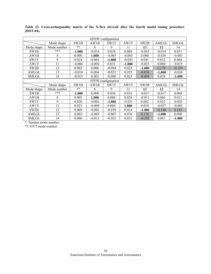
26American Institute of Aeronautics and Astronautics
Table 23. Cross-orthogonality matrix of the X-56A aircraft after the fourth model tuning procedure (DOT-04).
EFEW configurationMode shape SW1B AW1B SW1T AW1T SW2B AMLGL SMLGL
Mode shape Mode number 7* 8 9 11 13 12 14SW1B 7** -1.000 -0.016 0.038 0.009 -0.063 -0.014 0.051AW1B 8 0.000 1.000 -0.005 -0.005 0.000 -0.038 -0.003SW1T 9 0.024 -0.001 -1.000 -0.043 0.041 0.012 0.064AW1T 11 -0.006 -0.002 0.031 -1.000 -0.023 0.060 -0.015SW2B 12 0.002 0.006 -0.094 0.023 -1.000 0.179 -0.150
AMLGL 13 -0.010 0.004 -0.022 0.055 -0.058 -1.000 -0.036SMLGL 14 -0.015 0.003 -0.060 0.023 -0.004 0.038 -1.000
FFFW configurationMode shape SW1B AW1B SW1T AW1T SW2B AMLGL SMLGL
Mode shape Mode number 7* 8 9 11 13 12 14SW1B 7** -1.000 0.008 0.036 0.016 -0.037 -0.017 0.068AW1B 8 0.003 1.000 0.008 0.024 -0.011 0.066 0.011SW1T 9 0.020 0.004 -1.000 -0.031 0.062 0.022 0.028AW1T 11 0.023 -0.009 0.004 1.000 0.010 -0.037 -0.005SW2B 12 0.009 -0.001 -0.070 0.014 -1.000 -0.148 0.143
AMLGL 13 0.003 -0.003 -0.007 0.076 0.118 -1.000 0.000SMLGL 14 0.006 -0.011 -0.033 0.031 -0.292 0.061 -1.000
*: Nastran mode number**: GVT mode number

27American Institute of Aeronautics and Astronautics
Table 24. Design variable changes (%) during model tuning procedures.
Design variable Property Base† DOT1 DOT2 POH‡ DOT3 DOT41 CONM2* 100202 and 100204 Mass 0.0 0.8 0.8 13.4 17.6 7.92 PBAR** 310 I1 0.0 0.0 0.0 0.0 0.2 1.13 PBAR 313 I1 0.0 -1.4 -1.4 -8.5 8.9 11.74 PBAR 314 I1 0.0 -0.6 -0.6 -3.3 -10.4 -20.05 PBAR 308 I1 0.0 -0.5 -0.5 -2.0 -4.7 -12.96 PBAR 310 I2 0.0 0.3 0.3 -0.7 -4.5 -4.67 PBAR 313 I2 0.0 0.4 0.4 0.3 1.9 18.08 PBAR 310 J 0.0 0.0 0.0 0.0 -0.1 -0.19 PBAR 313 J 0.0 0.1 0.1 0.1 2.6 9.210 PBAR 314 J 0.0 0.4 0.4 0.4 6.4 20.011 PBUSH+ 315 and 316 K2 0.0 0.0 0.0 -0.5 -0.1 -1.612 PBUSH 315 and 316 K3 0.0 0.0 0.0 -0.7 -6.7 -4.213 PBUSH 315 and 316 K4 0.0 0.0 0.0 -0.5 -2.3 -4.914 MAT8++ 100 E 0.0 -2.0 -2.0 0.7 1.5 4.815 MAT8 100 G 0.0 6.4 6.4 9.0 13.9 17.916 PBAR 311 A 0.0 0.0 0.0 0.4 1.0 1.117 PBAR 312 A 0.0 0.0 0.0 2.3 9.0 15.318 PBAR 313 A 0.0 0.0 0.0 1.3 9.9 17.119 PBAR 312 I1 0.0 0.0 0.0 -0.1 0.5 1.020 PBAR 309 I1 0.0 0.0 0.0 -1.6 -6.3 -17.221 CONM2 930618 Mass 0.0 0.0 0.0 0.0 -1.9 -2.222 CONM2 9120105 Mass 0.0 0.0 0.0 1.2 -20.0 -20.023 CONM2 930668 Mass 0.0 0.0 0.0 -0.1 2.0 2.524 CONM2 9220105 Mass 0.0 0.0 0.0 -2.2 10.9 8.1†: Baseline configuration (tuned by LMSW)‡: Obtained from previous optimization history*: Concentrated mass element (MSC Nastran terminology)**: Simple beam property (MSC Nastran terminology)+: Generalized spring and damper property (MSC Nastran terminology)++: Shell element orthotropic material property (MSC Nastran terminology)

28American Institute of Aeronautics and Astronautics
Figures
Fig. 1. The X-56A aircraft with ground control stations. (Figure courtesy: AFRL/Lockheed Martin).
Fig. 2. Future research configurations of the X-56A aircraft.

29American Institute of Aeronautics and Astronautics
Fig. 3. Structural dynamic model tuning based on the object-oriented optimization (O3) tool.
Fig. 4. The X-56A aircraft with soft suspension system. (Photo courtesy: AFRL/Lockheed Martin).

30American Institute of Aeronautics and Astronautics
Fig. 5. Different models in this study.
Fig. 6. Finite element model of the X-56A aircraft.
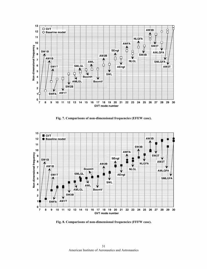
31American Institute of Aeronautics and Astronautics
Fig. 7. Comparisons of non-dimensional frequencies (EFEW case).
Fig. 8. Comparisons of non-dimensional frequencies (FFFW case).
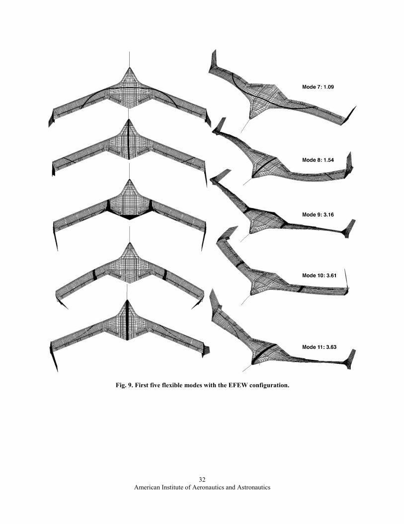
32American Institute of Aeronautics and Astronautics
Fig. 9. First five flexible modes with the EFEW configuration.

33American Institute of Aeronautics and Astronautics
Fig. 10. The unsteady aerodynamic model of the X-56A aircraft.

34American Institute of Aeronautics and Astronautics
Fig. 11. V-g and V-f curves of the X-56A baseline model with the EFEW at Mach = 0.16.

35American Institute of Aeronautics and Astronautics
Fig. 12. V-g and V-f curves of the X-56A final design model with the EFEW at Mach = 0.16.

36American Institute of Aeronautics and Astronautics
Fig. 13. Flutter boundaries and flight envelope of the X-56A aircraft under the EFEW configuration.
Fig. 14. The first three flutter mode shapes of the X-56A baseline model.

37American Institute of Aeronautics and Astronautics
Fig. 15. Summary of objective functions.
Fig. 16. Main landing gear model.

38American Institute of Aeronautics and Astronautics
Fig. 17. V-g and V-f curves of the X-56A aircraft after the fourth model tuning procedure (DOT-04) with the EFEW at Mach = 0.16.

39American Institute of Aeronautics and Astronautics
References
1Beranek, J., Nicolai, L., Buonanno, M., Burnett, E., Atkinson, C., Holm-Hansen, B., and Flick, P., “Conceptual Design of a Multi-utility Aeroelastic Demonstrator,” AIAA-2010-9350, 2010.
2Pak, C.-G. and Lung, S.-F., “Flutter Analysis of the Aerostructures Test Wing with Test Validated Structural Dynamic Model,” AIAA Journal of Aircraft, Vol. 48, No. 4, 2011, pp. 1263-1272.
3Pak, C.-G., “Unsteady Aerodynamic Model Tuning for Precise Flutter Prediction,” AIAA Journal of Aircraft,Vol. 48, No. 6, 2011, pp. 2178-2184.
4Lung, S.-F., and Pak, C.-G., “Updating the Finite Element Model of the Aerostructures Test Wing Using Ground Vibration Test Data,” NASA TM 2009-214646, 2009.
5Pak, C.-G., “Preliminary Development of an Object-Oriented Optimization Tool,” NASA TM 2011-216419, 2011.
6MSC/NASTRAN Quick Reference Guide Version 69, The MacNeal Schwendler Corporation, Newport Beach, California, 1996.
7DOT Design Optimization Tools User’s Manual Version 5.0, Vanderplaats Research and Development, Inc.,Colorado Springs, Colorado, 2001.
8Charbonneau, P., and Knapp, B., A User’s Guide to PIKAIA 1.0, National Center for Atmospheric Research, Boulder, Colorado, 1995.
9Erol, O. K., and Eksin, I., “A New Optimization Method: Big Bang-Big Crunch,” Advances in Engineering Software, Vol. 37, No. 2, 2006, pp. 106–111.
10Camp, C. V., “Design of Space Trusses using Big Bang-Big Crunch Optimization,” Journal of Structural Engineering, ASCE, Vol. 133, No. 7, 2007, pp. 999–1008.
11Kaveh, A., and Talatahari, S., “Size Optimization of Space Trusses Using Big Bang-Big Crunch Algorithm,” Computers and Structures, Vol. 87, No. 17-18, 2009, pp. 1129-1140.
12Tang, H., Zhou, J., Xue, S., and Xie, L., “Big Bang-Big Crunch Optimization for Parameter Estimation in Structural Systems,” Mechanical Systems and Signal Processing, Vol. 24, No. 8, 2010, pp. 2888-2897.
13Pak, C.-G., and Li, W., “Multidisciplinary Design, Analysis, and Optimization Tool Development Using a Genetic Algorithm,” Proceedings of the 26th International Congress of the Aeronautical Sciences, Anchorage, Alaska, 2008.
14O’Callahan, J., Avitabile, P., and Riemer, R., “System Equivalent Reduction Expansion Process,” Proceedings of the 7th International Modal Analysis Conference, Las Vegas, Nevada, 1989, pp. 29-37.
15Military Standard, “Test Requirements for Launch, Upper-stage, and Space Vehicles,” MIL-STD-1540C,Section 6.2.10, September 15, 1994.
16NASA Technical Standard, “Load Analysis of Spacecraft and Payloads,” NASA-STD-5002, Section 4.2.6.d, June 21, 1996.
17ZAERO User’s Manual Version 8.2, ZONA Technology, Inc., Scottsdale, Arizona, 2008.