cpu scheduling outline - ku ittcittc.ku.edu/~kulkarni/teaching/eecs678/slides/chap6.pdfcpu...

1

CPU Scheduling – Outline

What is scheduling in the OS ?

What are common scheduling criteria ?

How to evaluate scheduling algorithms ?

What are common scheduling algorithms ?

How is thread scheduling different from process scheduling ?

What are the issues in multiple-processor scheduling ?

Operating systems case studies.

2

Basic Concepts

Multiprogramming

most processes alternate between CPU bursts and I/O bursts

CPU free and idle during I/O burst

schedule another process on the CPU

maximizes CPU utilization

CPU bound process

spends most of its time in the CPU

at least a few long CPU bursts

I/O bound process

spends most its time performing I/O

several short CPU bursts

3

CPU Scheduler

Responsible for the selection of the next running process

part of the OS dispatcher

selects from among the processes in memory that are ready to execute

based on a particular strategy

When does CPU scheduling happen ?

process switches from running to waiting state

process switches from running to ready state

process switches from waiting to ready state

process terminates

Scheduling under 1 and 4 is nonpreemptive

All other scheduling is preemptive

4

Preemptive Vs. Non-preemptive CPU Scheduling

Non-preemptive scheduling

process voluntarily releases the CPU (conditions 1 and 4)

easy, requires no special hardware

poor response time for interactive and real-time systems

Preemptive scheduling

OS can force a running process involuntarily relinquish the CPU

arrival of a higher priority process

running process exceeds its time-slot

may require special hardware, eg., timer

may require synchronization mechanisms to maintain data consistency

complicates design of the kernel

favored by most OSes

5

Dispatcher

Scheduler is a part of the dispatcher module in the OS

Functions of the dispatcher

get the new process from the scheduler

switch out the context of the current process

give CPU control to the new process

jump to the proper location in the new program to restart that program

Time taken by the dispatcher to stop one process and start another running is called the dispatch latency

6

Scheduling Queues

Job queue: consists of all processes

all jobs (processes), once submitted, are in the job queue

scheduled by the long-term scheduler

Ready queue: consists of processes in memory

processes ready and waiting for execution

scheduled by the short-term or CPU scheduler

Device queue: processes waiting for a device

multiple processes can be blocked for the same device

I/O completion moves process back to ready queue

7

Scheduling Queues (2)

8

Performance Metrics for CPU Scheduling

CPU utilization: percentage of time that the CPU is busy

Throughput: number of processes that complete their execution per time unit

Turnaround time: amount of time to execute a particular process (submission time to completion time)

Waiting time: amount of time a process has been waiting in the ready queue

Response time: amount of time it takes from when a request was submitted until the first response is produced

Scheduling goals

maximize CPU utilization and throughput

minimize turnaround time, waiting time and response time

be fair to all processes and all users

9

Method for Evaluating CPU Scheduling Algorithms

Evaluation criteria

define relative importance of the performance metrics

include other system-specific measures

Deterministic modeling

takes a particular predetermined workload and defines the performance of each algorithm for that workload

simple and fast, gives exact numbers

difficult to generalize results

can recognize algorithm performance trends over several inputs

used for explaining scheduling algorithms

used in the rest of this chapter !

10

Workload Models and Gantt Charts

Workload model:

Gantt charts:

bar chart to illustrate a particular schedule

figure shows batch schedule

Process Arrival Time Burst Time

P1 0 8

P2 1 4

P3 1 10

P4 6 2

P1 P2 P3 P4

0 80 12 22 24

11

Deterministic Modeling Example

Suppose we have processes A, B, and C, submitted at time 0.

We want to know the response time, waiting time, and turnaround time of process A

A B C A B C A C A C Time

response time = 0+ +wait time

turnaround time

12



We want to know the response time, waiting time, and turnaround time of process B.


response time+wait time

turnaround time

13



We want to know the response time, waiting time, and turnaround time of process C


response time+ ++wait time

turnaround time

14

Method for Evaluating CPU Scheduling Algorithms (2)

Queueing models

analytically model the queue behavior (under some assumptions)

involves a lot of complicated math

can only handle a limited number of distributions and algorithms

may not be very accurate because of unrealistic assumptions

Simulations

get a workload information from a system

simulate the scheduling algorithm

compute the performance metrics

time and space intensive

is practically the best evaluation method

15

Simulation Illustration

16

Scheduling Algorithms

First Come, First Served (FCFS)

Shortest Job First (SJF)

Priority Based

Round Robin (RR)

Multilevel Queue Scheduling

Multilevel Feedback Queue Scheduling

17

First Come, First Served Scheduling

Assigns the CPU based on the order of the requests.

Implemented using a FIFO queue.

No preemption

Advantages

straightforward, simple to write and understand

Disadvantages

average waiting time may be too long

huge variation based on when processes arrive

cannot balance CPU-bound and I/O-bound processes

convoy effect, short process behind long process

cannot be used for time-sharing systems

18

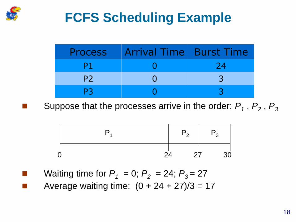
FCFS Scheduling Example

Suppose that the processes arrive in the order: P1 , P2 , P3

Waiting time for P1 = 0; P2 = 24; P3 = 27

Average waiting time: (0 + 24 + 27)/3 = 17

P1 P2 P3

24 27 300


P1 0 24

P2 0 3

P3 0 3

19

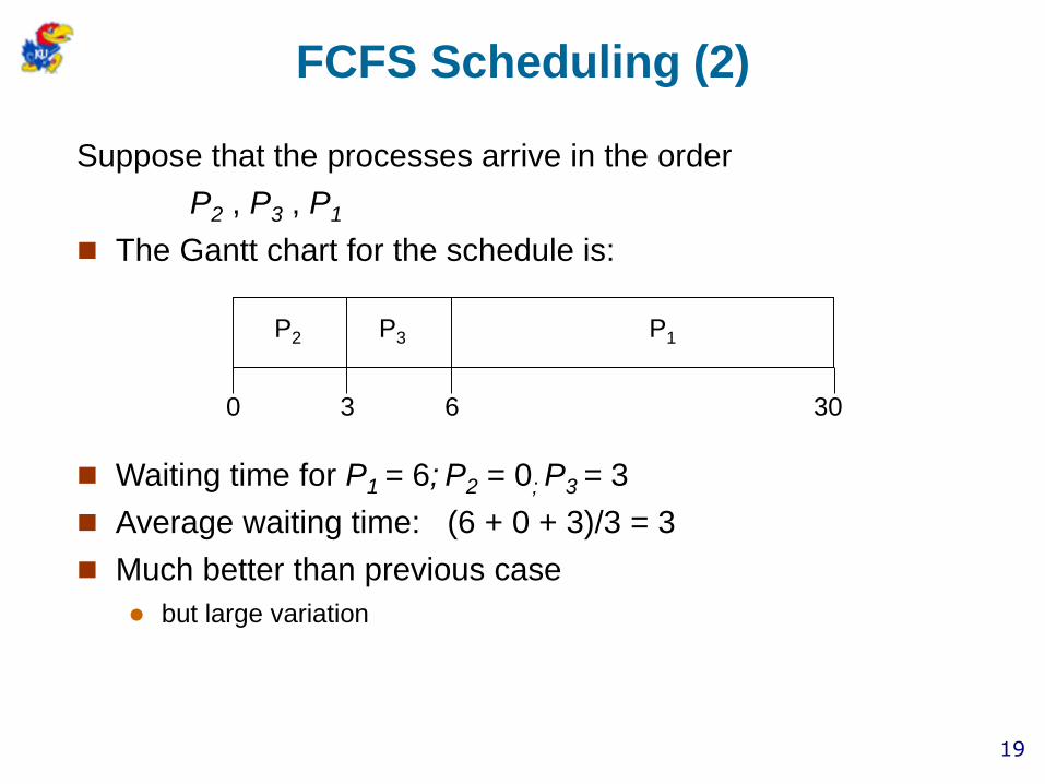
FCFS Scheduling (2)

Suppose that the processes arrive in the order

P2 , P3 , P1

The Gantt chart for the schedule is:

Waiting time for P1 = 6; P2 = 0; P3 = 3

Average waiting time: (6 + 0 + 3)/3 = 3

Much better than previous case

but large variation

P1P3P2

63 300

20

Shortest Job First (SJF) Scheduling

Order each process based on the length of its next CPU burst

Allocate CPU to the process from the front of the list

shortest next CPU burst

Advantages

SJF is optimal

achieves minimum average waiting time for a given set of processes

Disadvantages

difficult to know the length of the next CPU request

can ask the user, who may not know any better !

model-based prediction

can lead to process starvation

21

Example of SJF

SJF scheduling chart

Average waiting time = (3 + 16 + 9 + 0) / 4 = 7

P4P3P1

3 160 9

P2

24


P1 0 6

P2 0 8

P3 0 7

P4 0 3

22

Estimate Length of Next CPU Burst

Can only estimate the length

next CPU burst similar to previous CPU bursts ?

how relevant is the history of previous CPU bursts ?

Calculated as an exponential average of the previous CPU bursts for the process

Formula:

10 , 3.

burst CPUnext for the valuepredicted 2.

burst CPU oflength actual 1.

1

n

th

n nt

nnn t 1 1

23

Estimate Length of the Next CPU Burst (2)

=0

n+1 = n

Recent history does not count

=1

n+1 = tn

Only the actual last CPU burst counts

If we expand the formula, we get:

n+1 = tn+(1 - ) tn -1 + …

+(1 - )j tn -j + …

+(1 - )n +1 0

Since both and (1 - ) are less than or equal to 1, each successive term has less weight than its predecessor

24

Estimate Length of the Next CPU Burst (3)

25

Preemptive SJF Scheduling

New shorter process can preempt longer current running process

Shortest Remaining Time First scheduling chart:

Average waiting time = 6.5


P1 0 8

P2 1 4

P3 2 9

P4 3 5

P1

P2 P4 P1 P3

0 1 5 10 17 26

26

Priority Scheduling

A priority number associated with each process

CPU allocated to the process with the highest priority

equal priority processes scheduled in FCFS order

Internally determined priorities

time limit, memory requirements, etc

SJF uses next CPU burst for its priority (how?)

Externally specified priorities

process importance, user-level, etc

Can be preemptive or non-preemptive

Text uses low numbers for high priorities

27

Priority Scheduling (2)

Advantages

priorities can be made as general as needed

Disadvantage

low priority process may never execute (indefinite blocking or starvation)

Aging

technique to prevent starvation

increase priority of processes with time

28

Round Robin Scheduling (RR)

Round robin algorithm

arrange jobs in FCFS order

allocate CPU to the first job in the queue for one time-slice

preempt job, add it to the end of the queue

allocate CPU to the next job and continue...

One time slice is called a time quantum

Is by definition preemptive

can be considered as FCFS with preemption

Advantages

simple, avoids starvation

Disadvantages

may involve a large context switch overhead

higher average waiting time than SJF

an I/O bound process on a heavily loaded system will run slower

29

Example of RR with Time Quantum = 4

The Gantt scheduling chart is:

Average waiting time = 5.66

P1 P2 P3 P1 P1 P1 P1 P1

0 4 7 10 14 18 22 26 30

Process Burst Times

P1 24

P2 3

P3 3

30

Round Robin Scheduling (2)

Performance

depends on the length of the time quantum

large time quantum → FCFS like behavior

small time quantum → large context switch overhead

Generally,

time quanta range from 10 – 100 milliseconds

context switch time is less than 10 microseconds

RR has larger waiting time, but provides better response time for interactive systems

Turnaround time depends on the size of the time quantum

31

Turnaround Time Varies With The Time Quantum

32

Multilevel Queue

Ready queue is partitioned into separate queues:foreground (interactive)background (batch)

Each queue has its own scheduling algorithm

foreground – RR

background – FCFS

Scheduling must be done between the queues

Fixed priority scheduling; (i.e., serve all from foreground then from background). Possibility of starvation.

Time slice – each queue gets a certain amount of CPU time which it can schedule amongst its processes; i.e., 80% to foreground in RR, 20% to background in FCFS

33

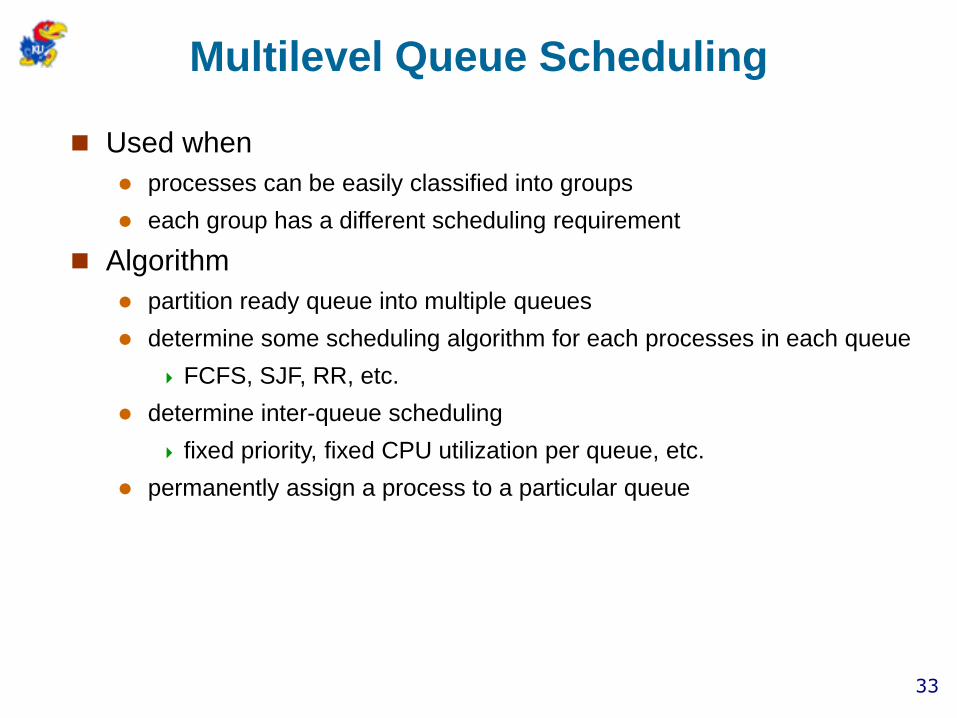
Multilevel Queue Scheduling

Used when

processes can be easily classified into groups

each group has a different scheduling requirement

Algorithm

partition ready queue into multiple queues

determine some scheduling algorithm for each processes in each queue

FCFS, SJF, RR, etc.

determine inter-queue scheduling

fixed priority, fixed CPU utilization per queue, etc.

permanently assign a process to a particular queue

34

Multilevel Queue Scheduling Example

Example: foreground Vs. background processes

foreground are interactive, background are batch processes

foreground have priority over background

intra-queue scheduling

foreground – response time, background – low overhead, no starvation

foreground – RR, background – FCFS

scheduling between the queues

fixed priority scheduling; foreground – higher priority

time slice; 80% to foreground in RR, 20% to background in FCFS

35

Multilevel Queue Scheduling Example (2)

36

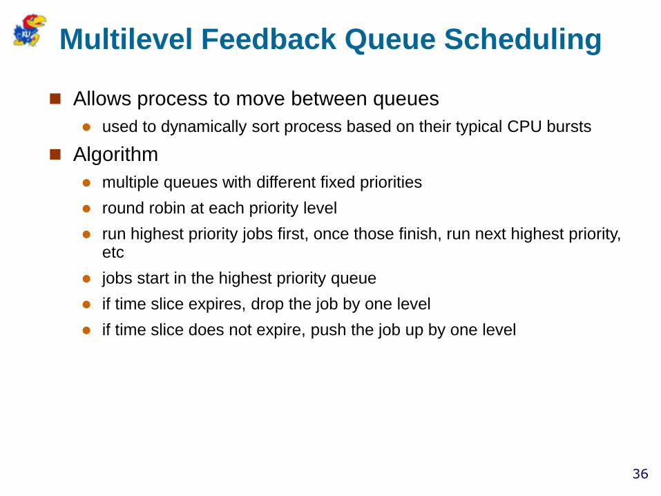
Multilevel Feedback Queue Scheduling

Allows process to move between queues

used to dynamically sort process based on their typical CPU bursts

Algorithm

multiple queues with different fixed priorities

round robin at each priority level

run highest priority jobs first, once those finish, run next highest priority, etc

jobs start in the highest priority queue

if time slice expires, drop the job by one level

if time slice does not expire, push the job up by one level

37

Example of Multilevel Feedback Queues

Priority 0 (time slice = 1):



time = 0

Time

A B C

0 2 5 9

38





time = 1

Time

A

B C

0

0 3 7

A

1

39





time = 2

Time

A B

C

0

0 4

3

A

1

B

40





time = 3

Time

A B C

0 63

A

1

B C

41





time = 3

Time

A B C

0 63

A

1

B C

Suppose A is blocked on I/O

42





time = 3

Time

A

B C

0

52

A

1

B C

Suppose A is blocked on I/O

0

43





time = 5

Time

A

B

C

0

3

A

1

B C

Suppose A now returns from I/O

0

44





time = 6

TimeAB

C

3

A B C

0

45





time = 8

TimeAB

C

3

A B C

0

C

46





time = 9

TimeAB CA B C C

47

Multilevel Feedback Queues

Approximates SRTF

a CPU-bound job drops like a rock

I/O-bound jobs stay near the top

Still unfair for long running jobs

counter-measure: Aging

increase the priority of long running jobs if they are not serviced for a period of time

tricky to tune aging

48

Lottery Scheduling

Adaptive scheduling approach to address the fairness problem

Algorithm

each process owns some tickets

on each time slice, a ticket is randomly picked

on average, the allocated CPU time is proportional to the number of tickets given to each job

To approximate SJF, short jobs get more tickets

To avoid starvation, each job gets at least one ticket

49

Lottery Scheduling Example

Short jobs: 10 tickets each

Long jobs: 1 ticket each

# short jobs/# long jobs

% of CPU for each short job

% of CPU for each long job

1/1 91% 9%

0/2 0% 50%

2/0 50% 0%

10/1 10% 1%

1/10 50% 5%

50

Thread Scheduling

On systems supporting threads

kernel threads are the real scheduling entities

user threads need to be mapped to kernel threads for execution

scheduling attributes may be set at thread creation

Contention-scope

PTHREAD_SCOPE_PROCESS

group user threads to contend for common kernel thread(s)

PTHREAD_SCOPE_SYSTEM

directly assign to kernel thread, contends with other kernel threads

inheritsched

PTHREAD_INHERIT_SCHED

inherit scheduling policy and priority from parent thread

PTHREAD_EXPLICIT_SCHED

explicitly specify scheduling policy and priority of the new thread

51

Thread Scheduling (2)

schedpolicy

SCHED_OTHER

regular non-real-time scheduling

SCHED_RR

real-time round-robin scheduling

SCHED_FIFO

real-time FCFS scheduling

schedparam

set/get the priority of the thread

All parameters only relevant

if thread library supports non-one-to-one user level threads

for real-time scheduling

52

Pthread Scheduling Example

int main(int argc, char *argv[]){

int i;

pthread t tid[5];

pthread attr t attr;

pthread attr init(&attr); /* get the default attributes */

/* set the scheduling algorithm to PROCESS or SYSTEM */

pthread attr setscope(&attr, PTHREAD SCOPE SYSTEM);

/* set the scheduling policy - FIFO, RT, or OTHER */

pthread attr setschedpolicy(&attr, SCHED OTHER);

for (i = 0; i < 5; i++)

pthread create(&tid[i],&attr,runner,NULL);

for (i = 0; i < NUM THREADS; i++)

pthread join(tid[i], NULL);

}

void *runner(void *param){

printf("I am a thread\n");

pthread exit(0);

}

53

Multiple-Processor Scheduling Issues

Multiprocessor Scheduling

asymmetric multiprocessing

only one processor accesses the system data structures

simple

symmetric multiprocessing (SMP)

each processor is self-scheduling

need to maintain scheduler data structures synchronization

Processor affinity

process has affinity for processor on which it is currently running

reduce memory and cache overhead

memory affinity important for NUMA architectures

soft and hard processor affinity

how strictly OS maintains affinity policy

54

NUMA and CPU Scheduling

55

Multiple-Processor Scheduling Issues

Load balancing

keep workload evenly distributed across all CPUs

important if each processor has its own queue of ready processes

push and pull migration

push or pull tasks towards idle processors

Multicore processors

multiple processor cores on same physical chip

uniform memory access, faster intercore communication

may be simultaneously multithreaded (SMT, or hyperthreaded)

instructions from multiple threads simultaneously live in different pipeline stages

OS given a view of one processor per hardware thread

may reduce memory stalls

may increase resource contention

56

Case Studies: Solaris Scheduling

Priority-based scheduling

Six classes

real time, system, fair share, fixed priority, time shar, and interactive

(in order of priority)

different priorities and scheduling algorithms in different classes

The default class is time sharing

uses multilevel feedback queue with variable time slices

inverse relationship between priorities and time slices

good response time for interactive processes and good throughput for CPU-bound processes

see the dispatch table

57

Solaris Dispatch Table

58

Case Studies: Solaris Scheduling (2)

Real-time scheduling class

highest priority, bounded time response

should be careful before putting a process in this class

System scheduling class

reserved for kernel threads (scheduling and paging daemon)

Fixed priority scheduling class

priorities not dynamically adjusted

Fair share scheduling class

based on lottery scheduling

processes grouped into projects; each project assigned some nubmer of lottery tokens

processes within each project share the token fairly

Process class priorities converted to global priorities

59

Map to Global Priorities

60

Case Studies: Linux Scheduling (v2.5)

Linux scheduling (version 2.5)

constant order O(1) scheduling time

support for SMP systems

provide fairness and support for interactive tasks

Priority-based, preemptive, global round-robin scheduling

two priority ranges: time-sharing and real-time

Real-time range from 0 to 99 and nice value from 100 to 140

numerically lower values have higher priorities

higher priority tasks are give longer time slice

Task run-able as long as time left in time slice (active)

If no time left (expired), not run-able until all other tasks use their slices

see mapping figure

61

Priorities and Time-slice length

62


More about Linux scheduling

maintains two arrays: active and expired

tasks linked in arrays according to their priorities

active tasks on expiration of their time quanta move to the expired array

real-time tasks have static priorities

normal tasks have dynamic priorities

63


Even more about Linux scheduling

After the time slice of a process is used up, the process must wait until all ready processes to use up their time slice (or be blocked)

round-robin approach

no starvation problem

for a user process, its priority may + or – 5 depending whether the process is I/O- bound or CPU-bound

I/O bound process is given higher priority

64

Case Studies: Linux Scheduling (v2.6.23+)

Completely Fair Scheduler (CFS)

Scheduling classes, each with specific priority

scheduler picks highest priority task in highest scheduling class

rather than quantum based on fixed time allotments, based on proportion of CPU time

two scheduling classes included (default, real-time), others can be added

Quantum calculated based on nice value from -20 to +19

lower value is higher priority

calculates target latency – interval of time during which task should run at least once

target latency can increase if say number of active tasks increases

CFS scheduler maintains per task virtual run time in variable vruntime

associated with decay factor based on priority of task

lower priority is higher decay rate

normal default priority yields virtual run time = actual run time

task with lowest virtual run time runs next

65

Case Studies: Linux Scheduling (v2.6.23+)

66

Case Studies: Summary

Basic idea for schedule user processes is the same for all systems

lower priority for CPU bound process

increase priority for I/O bound process

The scheduling in Solaris / Linux is more concerned about fairness

more popular as the OSes for servers

The scheduling in Window XP is more concerned about user perceived performance

more popular as the OS for personal computers

cpu scheduling outline - ku ittcittc.ku.edu/~kulkarni/teaching/eecs678/slides/chap6.pdfcpu...

Documents