cpu scheduling - operating system design mosig 1
TRANSCRIPT

CPU SchedulingOperating System Design – MOSIG 1
Instructor: Arnaud LegrandClass Assistants: Benjamin Negrevergne, Sascha Hunold
November 16, 2010
A. Legrand CPU Scheduling — 1 / 45

CPU Scheduling
I The scheduling problem:I Have K jobs ready to runI Have N ≥ 1 CPUsI Which jobs to assign to which CPU(s)
I When do we make decision?
A. Legrand CPU Scheduling — 2 / 45

CPU Scheduling
I Scheduling decisions may take place when a process:1. Switches from running to waiting state2. Switches from running to ready state3. Switches from waiting to ready4. Exits
I Non-preemptive schedules use 1 & 4 only
I Preemptive schedulers run at all four points
A. Legrand CPU Scheduling — 3 / 45

Criteria: Intuitive Notion
CPU utilization (max) percent usage of CPU.
Only useful computations(mix CPU, I/O; preemption overhead).
Throughput (max) average number of tasks that complete their executionper time-unit.
Turnaround Time/Response Time/Flow (min) amount of time it takes be-tween the task arrival and its completion.
Waiting Time (min) amount of time spent waiting for being executed.
Slowdown/Stretch (min) slowdown factor encountered by a task relativeto the time it would take on an unloaded system.
The previous quantities are task- or CPU-centric and need to be aggregatedinto a single objective function.
I max (the worst case)I average: arithmetic (i.e. sum)
or something else. . .
I variance (to be “fair” betweenthe tasks).
A. Legrand CPU Scheduling — 4 / 45

Criteria: Intuitive Notion
CPU utilization (max) percent usage of CPU. Only useful computations(mix CPU, I/O; preemption overhead).
Throughput (max) average number of tasks that complete their executionper time-unit.
Turnaround Time/Response Time/Flow (min) amount of time it takes be-tween the task arrival and its completion.
Waiting Time (min) amount of time spent waiting for being executed.
Slowdown/Stretch (min) slowdown factor encountered by a task relativeto the time it would take on an unloaded system.
The previous quantities are task- or CPU-centric and need to be aggregatedinto a single objective function.
I max (the worst case)I average: arithmetic (i.e. sum)
or something else. . .
I variance (to be “fair” betweenthe tasks).
A. Legrand CPU Scheduling — 4 / 45

Criteria: Classical Definitions
A given task Ti is defined by:I processing time pi
I release date ri
I (number of required processors qi )
I (deadline di )
Then, depending on the scheduling decision, we obtain its comple-tion time Ci
Completion Time
I Makespan: Cmax = maxi Ci
This metric is relevant when scheduling a single application(made of several synchronized process).
I Total (or average) Completion Time: SC =∑
i Ci
A. Legrand CPU Scheduling — 5 / 45

Criteria: Classical Definitions
A given task Ti is defined by:I processing time pi
I release date ri
I (number of required processors qi )
I (deadline di )
Then, depending on the scheduling decision, we obtain its comple-tion time Ci
Response TimeFi = Ci − ri
I Maximum Flow Time: Fmax = maxi Fi
I Total Completion Time: SF =∑
i Fi = SC −∑
i ri
A. Legrand CPU Scheduling — 5 / 45

Criteria: Classical Definitions
A given task Ti is defined by:I processing time pi
I release date ri
I (number of required processors qi )
I (deadline di )
Then, depending on the scheduling decision, we obtain its comple-tion time Ci
Waiting TimeWi = Ci − ri − pi
I Maximum Waiting time: Wmax = maxi Wi
I Total Waiting Time: SW =∑
i Wi = SF −∑
i pi
A. Legrand CPU Scheduling — 5 / 45
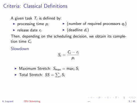
Criteria: Classical Definitions
A given task Ti is defined by:I processing time pi
I release date ri
I (number of required processors qi )
I (deadline di )
Then, depending on the scheduling decision, we obtain its comple-tion time Ci
Slowdown
Si =Ci − ri
pi
I Maximum Stretch: Smax = maxi Si
I Total Stretch: SS =∑
i Si
A. Legrand CPU Scheduling — 5 / 45

Outline
Optimizing largest response time
Optimizing throughput
Optimizing average response time
Avoiding starvation
Coming up with a compromise
Recap
A. Legrand CPU Scheduling — 6 / 45

Outline
Optimizing largest response time
Optimizing throughput
Optimizing average response time
Avoiding starvation
Coming up with a compromise
Recap
A. Legrand CPU Scheduling Optimizing largest response time — 7 / 45

Let’s play with a small example
We wish to find a schedule (possibly using preemption) that has thesmallest possible max flow (maxi Ci − ri ).
First-Come First-Served seems to be optimal.
A. Legrand CPU Scheduling Optimizing largest response time — 8 / 45

Let’s play with a small example
We wish to find a schedule (possibly using preemption) that has thesmallest possible max flow (maxi Ci − ri = 12).
First-Come First-Served seems to be optimal.
A. Legrand CPU Scheduling Optimizing largest response time — 8 / 45

FCFS is optimal: sketch of the proof
Proof:
I Let us consider an optimal schedule σ. Let us assume thatthere are two jobs A and B that are not scheduled accordingto the FCFS policy, i.e. rB < rA and CA < CB .
I By scheduling B before A, we do not increase max(CA−rA,CB−rB).
I Therefore, by scheduling A and B according to the FCFS policy,we get a new schedule σ′ that is still optimal.
I By proceeding similarly for all pairs of jobs, we prove that FCFSis optimal. �
rB rA CA CB
A. Legrand CPU Scheduling Optimizing largest response time — 9 / 45

FCFS is optimal: sketch of the proof
Proof:
I Let us consider an optimal schedule σ. Let us assume thatthere are two jobs A and B that are not scheduled accordingto the FCFS policy, i.e. rB < rA and CA < CB .
I By scheduling B before A, we do not increase max(CA−rA,CB−rB).
I Therefore, by scheduling A and B according to the FCFS policy,we get a new schedule σ′ that is still optimal.
I By proceeding similarly for all pairs of jobs, we prove that FCFSis optimal. �
rB rA CACB
A. Legrand CPU Scheduling Optimizing largest response time — 9 / 45

FCFS is optimal: sketch of the proof
Proof:
I Let us consider an optimal schedule σ. Let us assume thatthere are two jobs A and B that are not scheduled accordingto the FCFS policy, i.e. rB < rA and CA < CB .
I By scheduling B before A, we do not increase max(CA−rA,CB−rB).
I Therefore, by scheduling A and B according to the FCFS policy,we get a new schedule σ′ that is still optimal.
I By proceeding similarly for all pairs of jobs, we prove that FCFSis optimal. �
We do not even need to preempt jobs! Note that when you havemore than one processor, things are more complicated:
Bad News NP-complete with no preemption.
Good news Polynomial algorithm with preemption but it is muchmore complicated than FCFS.
A. Legrand CPU Scheduling Optimizing largest response time — 9 / 45

FCFS: other criteriaI The FCFS scheduling policy is non-clairvoyant, easy to
implement, and does not use preemption.
I The FCFS policy is optimal for minimizing max Fi . It min-imizes the “response time”!Yet, would you say it is “reactive” ?
I Run jobs in order that they arriveI E.g.., Say P1 needs 24 sec, while P2 and P3 need 3.I Say P2, P3 arrived immediately after P1, get:
I Throughput: 3 jobs / 30 sec = 0.1 jobs/secI Turnaround Time: P1 : 24, P2 : 27, P3 : 30
I Average TT: (24 + 27 + 30)/3 = 27
I Can we do better?
A. Legrand CPU Scheduling Optimizing largest response time — 10 / 45

FCFS continued
I We would accept to sacrifice some jobs to get somethingmore “reactive”.
I Suppose we scheduled P2, P3, then P1
I Would get:
I Throughput: 3 jobs / 30 sec = 0.1 jobs/secI Turnaround time: P1 : 30, P2 : 3, P3 : 6
I Average TT: (30 + 3 + 6)/3 = 13 – much less than 27
I Lesson: scheduling algorithm can reduce TT
I What about throughput?
A. Legrand CPU Scheduling Optimizing largest response time — 11 / 45

Outline
Optimizing largest response time
Optimizing throughput
Optimizing average response time
Avoiding starvation
Coming up with a compromise
Recap
A. Legrand CPU Scheduling Optimizing throughput — 12 / 45

View CPU and I/O devices the same
I CPU is one of several devices needed by users’ jobsI CPU runs compute jobs, Disk drive runs disk jobs, etc.I With network, part of job may run on remote CPU
I Scheduling 1-CPU system with n I/O devices like schedul-ing asymmetric n + 1-CPU multiprocessor
I Result: all I/O devices + CPU busy =⇒ n+1 fold speedup!
I Overlap them just right? throughput will be almost doubled
A. Legrand CPU Scheduling Optimizing throughput — 13 / 45

Bursts of computation & I/O
I Jobs contain I/O and computationI Bursts of computationI Then must wait for I/O
I To Maximize throughputI Must maximize CPU utilizationI Also maximize I/O device utilization
I How to do?I Overlap I/O & computation from multiple
jobsI Means response time very important for
I/O-intensive jobs: I/O device will be idleuntil job gets small amount of CPU to is-sue next I/O request
A. Legrand CPU Scheduling Optimizing throughput — 14 / 45
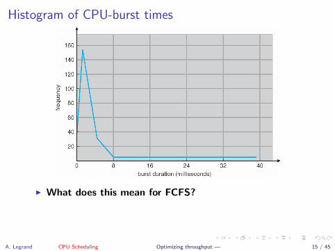
Histogram of CPU-burst times
I What does this mean for FCFS?
A. Legrand CPU Scheduling Optimizing throughput — 15 / 45

FCFS Convoy effect
I CPU bound jobs will hold CPU until exit or I/O(but I/O rare for CPU-bound thread)
I long periods where no I/O requests issued, and CPU heldI Result: poor I/O device utilization
I Example: one CPU-bound job, many I/O boundI CPU bound runs (I/O devices idle)I CPU bound blocksI I/O bound job(s) run, quickly block on I/OI CPU bound runs againI I/O completesI CPU bound job continues while I/O devices idle
I Simple hack: run process whose I/O completed?I What is a potential problem?
A. Legrand CPU Scheduling Optimizing throughput — 16 / 45

Outline
Optimizing largest response time
Optimizing throughput
Optimizing average response time
Avoiding starvation
Coming up with a compromise
Recap
A. Legrand CPU Scheduling Optimizing average response time — 17 / 45

Let’s play with a small example
We wish to find a schedule (possibly using preemption) that has thesmallest possible sum flow (
∑i Ci − ri ).
Shortest Remaining Processing Timer first seems to be optimal.
A. Legrand CPU Scheduling Optimizing average response time — 18 / 45

Let’s play with a small example
We wish to find a schedule (possibly using preemption) that has thesmallest possible sum flow (
∑i Ci − ri = 28).
Shortest Remaining Processing Timer first seems to be optimal.
A. Legrand CPU Scheduling Optimizing average response time — 18 / 45

SRPT is optimal: sketch of the proof
I Let us consider an optimal schedule σ. Let us assume thatthere are two jobs A and B that are not scheduled according tothe SRPT policy, i.e. CA < CB and at some point there weremore work to finish A than to finish B.
I By scheduling B before A, we strictly decrease CA + CB andthus we strictly decrease the total flow.
I Therefore, the original schedule was not optimal! The onlyoptimal schedule is thus SRPT. �
Decision CA CB
A. Legrand CPU Scheduling Optimizing average response time — 19 / 45

SRPT is optimal: sketch of the proof
I Let us consider an optimal schedule σ. Let us assume thatthere are two jobs A and B that are not scheduled according tothe SRPT policy, i.e. CA < CB and at some point there weremore work to finish A than to finish B.
I By scheduling B before A, we strictly decrease CA + CB andthus we strictly decrease the total flow.
I Therefore, the original schedule was not optimal! The onlyoptimal schedule is thus SRPT. �
Decision CB CA
A. Legrand CPU Scheduling Optimizing average response time — 19 / 45

SRPT is optimal: sketch of the proof
I Let us consider an optimal schedule σ. Let us assume thatthere are two jobs A and B that are not scheduled according tothe SRPT policy, i.e. CA < CB and at some point there weremore work to finish A than to finish B.
I By scheduling B before A, we strictly decrease CA + CB andthus we strictly decrease the total flow.
I Therefore, the original schedule was not optimal! The onlyoptimal schedule is thus SRPT. �
Here, preemption is required!
Bad News NP-complete for multiple processors or with no preemp-tion.
Good News Algorithm with logarithmic competitive ratio on multi-ple processors exists.
A. Legrand CPU Scheduling Optimizing average response time — 19 / 45

Comments
I Scheduling small jobs first is good for “reactivity” but it requiresto know the size of the jobs (i.e. clairvoyant).
I Scheduling small jobs first is good for the average response timebut some jobs may be left behind. . .
I Do you know an algorithm where job cannot starve?
A. Legrand CPU Scheduling Optimizing average response time — 20 / 45

Comments
I Scheduling small jobs first is good for “reactivity” but it requiresto know the size of the jobs (i.e. clairvoyant).
I Scheduling small jobs first is good for the average response timebut large jobs may be left behind. . .
I Do you know an algorithm where job cannot starve?
A. Legrand CPU Scheduling Optimizing average response time — 20 / 45

FCFS is ∆-competitive for∑
Fi
∆: ratio of the sizes of the largest and smallest job.Let’s prove FCFS is at most ∆-competitive.
FCFS is at exactly ∆-competitive.
A. Legrand CPU Scheduling Optimizing average response time — 21 / 45

FCFS is ∆-competitive for∑
Fi
∆: ratio of the sizes of the largest and smallest job.Let’s prove FCFS is at most ∆-competitive.
n
∆
n2
1/n
FCFS is at exactly ∆-competitive.
A. Legrand CPU Scheduling Optimizing average response time — 21 / 45

FCFS is ∆-competitive for∑
Fi
∆: ratio of the sizes of the largest and smallest job.Let’s prove FCFS is at most ∆-competitive.
n
∆
n2
1/n
SFFCFS = ∆ + ...+ n∆ + n2
(1 + n∆− 1
n
)=
2n3∆ + n2(2 + ∆) + n(∆− 2)
2
FCFS is at exactly ∆-competitive.
A. Legrand CPU Scheduling Optimizing average response time — 21 / 45

FCFS is ∆-competitive for∑
Fi
∆: ratio of the sizes of the largest and smallest job.Let’s prove FCFS is at most ∆-competitive.
n
∆
n2
1/nSFSRPT = n2 × 1 + (n2 + ∆) + ...+ (n2 + n∆)
= n3 + n2 +n(n + 1)
2∆
FCFS is at exactly ∆-competitive.
A. Legrand CPU Scheduling Optimizing average response time — 21 / 45

FCFS is ∆-competitive for∑
Fi
∆: ratio of the sizes of the largest and smallest job.Let’s prove FCFS is at most ∆-competitive.
n
∆
n2
1/n
%FCFS(∆) >SFFCFS
SFSRPT=
2n3∆+n2(2+∆)+n(∆−2)2
n3 + n2 + n(n+1)2 ∆
=2n3∆ + n2(2 + ∆) + n(∆− 2)
2n3 + 2n2 + n(n + 1)∆−−−−→n→+∞
∆
FCFS is at exactly ∆-competitive.
A. Legrand CPU Scheduling Optimizing average response time — 21 / 45

Optimizing the average response time with no starvation?
TheoremConsider any online algorithm whose competitive ratio for averageflow minimization satisfies %(∆) < ∆.
There exists for this algorithm a sequence of jobs leading tostarvation, and for which the maximum flow can be as far as wewant from the optimal maximum flow.
The starvation issue is inherent to the optimization of the averageresponse time.Still, we would like something “reactive” and we like the idea thatshort jobs have a higher priority.
A. Legrand CPU Scheduling Optimizing average response time — 22 / 45

Recap SJF/SRPT limitations
I The previous analysis relies on a model (i.e. a simplifica-tion of reality) and is thus limited.
I Actually, in practice, doesn’t always minimize averageturnaround time
I Example where turnaround time might be suboptimal?
If applications are made of jobs/tasks that have dependencies(synchronizations), if more than 1 CPU, . . .
I Can lead to unfairness or starvation
I In practice, can’t actually predict the futureI But can estimate CPU burst length based on past
I Exponentially weighted average a good ideaI tn actual length of proc’s nth CPU burstI τn+1 estimated length of proc’s n + 1st
I Choose parameter α where 0 < α ≤ 1I Let τn+1 = αtn + (1− α)τn
A. Legrand CPU Scheduling Optimizing average response time — 23 / 45
Recap SJF/SRPT limitations
I The previous analysis relies on a model (i.e. a simplifica-tion of reality) and is thus limited.
I Actually, in practice, doesn’t always minimize averageturnaround time
I Example where turnaround time might be suboptimal?If applications are made of jobs/tasks that have dependencies(synchronizations), if more than 1 CPU, . . .
I Can lead to unfairness or starvation
I In practice, can’t actually predict the futureI But can estimate CPU burst length based on past
I Exponentially weighted average a good ideaI tn actual length of proc’s nth CPU burstI τn+1 estimated length of proc’s n + 1st
I Choose parameter α where 0 < α ≤ 1I Let τn+1 = αtn + (1− α)τn
A. Legrand CPU Scheduling Optimizing average response time — 23 / 45
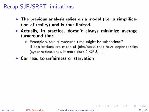

Exp. weighted average example
A. Legrand CPU Scheduling Optimizing average response time — 24 / 45

Outline
Optimizing largest response time
Optimizing throughput
Optimizing average response time
Avoiding starvation
Coming up with a compromise
Recap
A. Legrand CPU Scheduling Avoiding starvation — 25 / 45
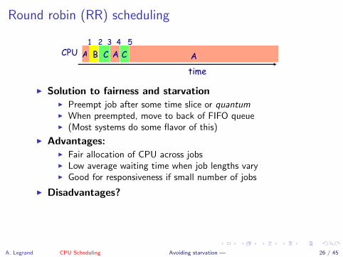
Round robin (RR) scheduling
I Solution to fairness and starvationI Preempt job after some time slice or quantumI When preempted, move to back of FIFO queueI (Most systems do some flavor of this)
I Advantages:I Fair allocation of CPU across jobsI Low average waiting time when job lengths varyI Good for responsiveness if small number of jobs
I Disadvantages?
A. Legrand CPU Scheduling Avoiding starvation — 26 / 45

RR disadvantages
I Varying sized jobs are good. . . but what about same-sized jobs?
I Assume 2 jobs of time=100 each:
I What is average completion time?I How does that compare to FCFS?
I In the previous algorithms (FCFS, SRPT), we have neverproduced a schedule with . . .A . . .B . . .A . . .B . . . . Intu-itively alternating jobs is not a good idea for minimizingcompletion time.
I Preemption should not be blindly used to ensure fairness.It should help to deal with the online non-clairvoyant set-ting.
A. Legrand CPU Scheduling Avoiding starvation — 27 / 45

Context switch costsI What is the cost of a context switch? (recall from previ-
ous lectures)
I Brute CPU time cost in kernelI Save and restore resisters, etc.I Switch address spaces (expensive instructions)
I Indirect costs: cache, buffer cache, & TLB misses
A. Legrand CPU Scheduling Avoiding starvation — 28 / 45

Time quantum
I How to pick quantum?I Want much larger than context switch costI Majority of bursts should be less than quantumI But not so large system reverts to FCFS
I Typical values: 10–100 msec
A. Legrand CPU Scheduling Avoiding starvation — 29 / 45

Turnaround time vs. quantum
A. Legrand CPU Scheduling Avoiding starvation — 30 / 45

Two-level scheduling
I Switching to swapped out process very expensiveI Swapped out process has most pages on diskI Will have to fault them all in while runningI One disk access costs ∼10ms. On 1GHz machine, 10ms = 10
million cycles!
I Context-switch-cost aware schedulingI Run in-core subset for “a while”I Then swap some between disk and memory
I How to pick subset? How to define “a while”?I View as scheduling memory before CPUI Swapping in process is cost of memory “context switch”I So want “memory quantum” much larger than swapping cost
A. Legrand CPU Scheduling Avoiding starvation — 31 / 45

Outline
Optimizing largest response time
Optimizing throughput
Optimizing average response time
Avoiding starvation
Coming up with a compromise
Recap
A. Legrand CPU Scheduling Coming up with a compromise — 32 / 45
Priority scheduling
I Associate a numeric priority with each processI E.g., smaller number means higher priority (Unix/BSD)I Or smaller number means lower priority (Pintos)
I Give CPU to the process with highest priorityI Can be done preemptively or non-preemptively
I Note SJF is a priority scheduling where priority is thepredicted next CPU burst time
I Starvation – low priority processes may never executeI Solution?
I Aging - increase a process’s priority as it waits
A. Legrand CPU Scheduling Coming up with a compromise — 33 / 45

Multilevel feeedback queues (BSD)
I Every runnable process on one of 32 run queuesI Kernel runs process on highest-priority non-empty queueI Round-robins among processes on same queue
I Process priorities dynamically computedI Processes moved between queues to reflect priority changesI If a process gets higher priority than running process, run it
I Idea: Favor interactive jobs that use less CPU
A. Legrand CPU Scheduling Coming up with a compromise — 34 / 45

Process priority
I p nice – user-settable weighting factorI p estcpu – per-process estimated CPU usage
I Incremented whenever timer interrupt found proc. runningI Decayed every second while process runnable
p estcpu←(
2 · load2 · load + 1
)p estcpu + p nice
I Load is sampled average of length of run queue plus short-termsleep queue over last minute
I Run queue determined by p usrpri/4
p usrpri← 50 +(p estcpu
4
)+ 2 · p nice
(value clipped if over 127)
A. Legrand CPU Scheduling Coming up with a compromise — 35 / 45

Sleeping process increases priority
I p estcpu not updated while asleepI Instead p slptime keeps count of sleep time
I When process becomes runnable
p estcpu←(
2 · load2 · load + 1
)p slptime
× p estcpu
I Approximates decay ignoring nice and past loads
I These are uggly hacks.I The BSD time quantum: 1/10 sec (since ∼1980)I Empirically longest tolerable latencyI Computers now faster, but job queues also shorter
A. Legrand CPU Scheduling Coming up with a compromise — 36 / 45

Limitations of BSD scheduler
I Hard to have isolation / prevent interferenceI Priorities are absolute
I Can’t donate priority (e.g., to server on RPC)I No flexible control
I E.g., In monte carlo simulations, error is 1/sqrt(N) after N trialsI Want to get quick estimate from new computationI Leave a bunch running for a while to get more accurate results
I Multimedia applicationsI Often fall back to degraded quality levels depending on resourcesI Want to control quality of different streams
A. Legrand CPU Scheduling Coming up with a compromise — 37 / 45

Real-time scheduling
I Two categories:I Soft real time—miss deadline and CD will sound funnyI Hard real time—miss deadline and plane will crash
I System must handle periodic and aperiodic eventsI E.g., procs A, B, C must be scheduled every 100, 200, 500 msec,
require 50, 30, 100 msec respectively
I Schedulable if∑ CPU
period≤ 1 (not counting switch time)
I Variety of scheduling strategiesI E.g., first deadline first (works if schedulable)
I Linux is finaly slightly moving from priority scheduling todeadline scheduling
A. Legrand CPU Scheduling Coming up with a compromise — 38 / 45

Multiprocessor scheduling issues
I Must decide on more than which processes to runI Must decide on which CPU to run which process
I Moving between CPUs has costsI More cache misses, depending on arch more TLB misses too
I Affinity scheduling—try to keep threads on same CPU
I But also prevent load imbalancesI Do cost-benefit analysis when deciding to migrate
A. Legrand CPU Scheduling Coming up with a compromise — 39 / 45

Multiprocessor scheduling (cont)
I Want related processes scheduled togetherI Good if threads access same resources (e.g., cached files)I Even more important if threads communicate often,
otherwise must context switch to communicate
I Gang scheduling—schedule all CPUs synchronouslyI With synchronized quanta, easier to schedule related processes/threads
together
A. Legrand CPU Scheduling Coming up with a compromise — 40 / 45

Outline
Optimizing largest response time
Optimizing throughput
Optimizing average response time
Avoiding starvation
Coming up with a compromise
Recap
A. Legrand CPU Scheduling Recap — 41 / 45

CPU Scheduling Recap
I Goal: High throughputI Minimize context switches to avoid wasting CPU, TLB misses,
cache misses, even page faults.
I Goal: Low latencyI People typing at editors want fast responseI Network services can be latency-bound, not CPU-bound
I AlgorithmsI Round-robinI Priority schedulingI Shortest process next (if you can estimate it)I Fair-Share Schedule (try to be fair at level of users, not pro-
cesses)I Fancy combinations of the above
A. Legrand CPU Scheduling Recap — 42 / 45

The universality of scheduling
I General problem: Let m requests share n resourcesI Always same issues: fairness, prioritizing, optimization
I Disk arm: which read/write request to do next?I Optimal: close requests = fasterI Fair: don’t starve far requests
I Memory scheduling: whom to take page from?I Optimal: past=future? take from least-recently-usedI Fair: equal share of memory
I Printer: what job to print?I People = fairness paramount: uses FIFO rather than SJFI Use “admission control” to combat long jobs
A. Legrand CPU Scheduling Recap — 43 / 45

How to allocate resources
I Space sharing (sometimes): split up. When to stop?I Time-sharing (always): how long do you give out piece?
I Pre-emptable (CPU, memory) vs. non-preemptable (locks, files,terminals)
A. Legrand CPU Scheduling Recap — 44 / 45
Postscript
I In principle, scheduling decisions can be arbitrary & shouldn’taffect program’s results
I Good, since rare that “the best” schedule can be calculated
I In practice, schedule does affect correctnessI Soft real time (e.g., mpeg or other multimedia) commonI Or after 10s of seconds, users will give up on web server
I Unfortunately, algorithms strongly affect system through-put, turnaround time, and response time
I The best schemes are adaptive. To do absolutely bestwe’d have to predict the future.
I Most current algorithms tend to give the highest priority to theprocesses that need the least CPU time
I Scheduling has gotten increasingly ad hoc over the years. 1960spapers very math heavy, now mostly “tweak and see”
A. Legrand CPU Scheduling Recap — 45 / 45