cpt, modified gravity and the baryon asymmetry of the universe · dos quais quebram tamb em a...
TRANSCRIPT

CPT,
Modified Gravity
and the Baryon
Asymmetry of the
UniverseMaria Pestana da Luz Pereira RamosMestrado em Física (Especialização Teórica)Departamento de Física e Astronomia
2017
Orientador Jorge Tiago Almeida Páramos, Professor Auxiliar Convidado,
Faculdade de Ciências da Universidade do Porto


Todas as correções determinadas
pelo júri, e só essas, foram efetuadas.
O Presidente do Júri,
Porto, ______/______/_________

“Tyger Tyger, burning bright,
In the forests of the night;
What immortal hand or eye,
Could frame thy fearful symmetry?”
– William Blake, The Tyger


Acknowledgements
First of all, I want to thank my supervisor, Jorge Paramos, for allowing me to study a subject I am
so interested in. Thank you for always being available to discuss my doubts while teaching me that every
professor should offer his students (a lot of) caffeine, if they choose to follow physics.
My gratitude to professor Orfeu Bertolami who has made a lot of research concerning the topics of
this thesis and who was readily available to discuss them with me. I would like also to thank the other
professors who were able to arouse my curiosity and clarify my ideas.
In these five years, I had the fortune to be in a room with people that I admire, who not only shared
their complete and deep vision of physics with me, but who also are kind human beings. For that, I am
truly grateful to Joao Pedro Pires, Joao Guerra, Antonio Antunes, Simao Joao and Bruno Madureira.
Last but not least, I thank my family for the endless patience, love and for giving me the opportunity
to do whatever I wanted, and my best friend, Beatriz Alvares Ribeiro, for the daily encouragement and
optimism throughout this period.


UNIVERSIDADE DO PORTO
Abstract
Departamento de Fısica e Astronomia
Faculdade de Ciencias da Universidade do Porto
Master of Science
CPT, Modified Gravity and the Baryon Asymmetry of the Universe
by Maria Pestana da Luz Pereira Ramos
The long-standing problem of the asymmetry between matter and antimatter in the Universe establishes a
deep connection between Cosmology, Quantum Field Theory and Particle Physics. In this work, we derive
a proof of the CPT Theorem, whose application justifies the existence and properties of antiparticles.
Furthermore, we show that the identification of CPT with the strong reflection operation allows to
formulate a framework where the Standard Model is extended to include Lorentz-violating terms, which
can lead to CPT-violating observable effects. We also review the present status of observations explaining
the observed baryon asymmetry, η, and the theoretical conditions for baryogenesis.
We study a class of models entailing violation of CPT symmetry in the early Universe, which allow
the generation of η while baryon violating forces are still in equilibrium. This can occur due to space-
time backgrounds which do not respect some of the assumptions for the validity of the CPT theorem. In
particular, we derive the amount of η that can be produced by the classical motion of a scalar field in its
potential, following Cohen and Kaplan’s model for spontaneous baryogenesis. Another way to generate
the observed asymmetry is to resort to modified gravity models, where the scalar field is replaced by the
Ricci scalar: we argue that f(R) gravity with a nonminimal geometry-matter coupling (NMC) naturally
points toward the transition from spontaneous to gravitational baryogenesis.
As a generalization of current models of f(R)-baryogenesis, we proceed by examining the allowed
region of variation for the mass scales and the exponents of both f(R) and NMC functions, showing that
tiny deviations from General Relativity are consistent with the observed baryon asymmetry and lead to
temperatures compatible with Big Bang Nucleosynthesis.


UNIVERSIDADE DO PORTO
Resumo
Departamento de Fısica e Astronomia
Faculdade de Ciencias da Universidade do Porto
Mestre de Ciencia
CPT, Gravidade Modificada e a Assimetria Barionica do Universo
por Maria Pestana da Luz Pereira Ramos
A existencia da assimetria cosmologica entre materia e antimateria, um problema frequentemente discu-
tido na literatura, estabelece uma conexao profunda entre a Cosmologia, a Teoria Quantica de Campo e
a Fısica de Partıculas. Neste trabalho, deriva-se uma prova do Teorema CPT, que justifica a existencia
e as propriedades das antipartıculas. Em particular, identificando esta operacao com a reflexao forte, e
possıvel generalizar o Modelo Padrao, de modo a incluir termos que violam a simetria de Lorentz, alguns
dos quais quebram tambem a invariancia CPT, levando a efeitos possivelmente acessıveis a experiencia.
Para alem disso, procede-se a revisao do estado corrente de observacoes que explicam a assimetria obser-
vacional, η, e das condicoes teoricas necessarias a bariogenese.
Estuda-se uma classe de modelos que admite uma violacao da simetria CPT no Universo primitivo,
permitindo a geracao de η, enquanto as interacoes que violam o numero barionico estao ainda em equilıbrio
termico. Este cenario e possıvel devido a introducao de potenciais, interpretados como fundos cosmicos,
que nao respeitam alguma das hipoteses do Teorema CPT. Especificamente, avalia-se a quantidade η
produzida devido ao movimento classico de um campo escalar ao longo de um potencial, seguindo o
modelo proposto por Cohen e Kaplan para o desenvolvimento de bariogenese espontanea. Uma forma
alternativa de gerar a assimetria barionica seria recorrer a modelos de gravidade modificada, substituindo
o campo escalar pelo escalar de Ricci: deste modo, argumenta-se que as teorias f(R) com um acoplamento
nao mınimo entre curvatura e materia (NMC) apontam, naturalmente, para a transicao de bariogenese
espontanea para gravitacional.
Generalizando trabalhos previos, que desenvolvem um mecanismo para a bariogenese no contexto das
teorias f(R), examina-se a regiao de variacao das escalas de massa e dos expoentes de ambas as funcoes
f(R) e NMC, concluindo que pequenos desvios da Relatividade Geral sao consistentes com a assimetria
barionica observada, sendo compatıveis com temperaturas caracterısticas da Nucleossıntese Primordial.


Contents
Acknowledgements 3
Abstract 5
Resumo 7
1 Introduction 1
2 CPT Invariance 3
2.1 Field Operators . . . . . . . . . . . . . . . . . . . . . . . . . . . . . . . . . . . . . . . . . . 3
2.2 Discrete Symmetries . . . . . . . . . . . . . . . . . . . . . . . . . . . . . . . . . . . . . . . 4
2.2.1 Parity . . . . . . . . . . . . . . . . . . . . . . . . . . . . . . . . . . . . . . . . . . . 4
2.2.2 Charge Conjugation . . . . . . . . . . . . . . . . . . . . . . . . . . . . . . . . . . . 6
2.2.3 Time Reversal . . . . . . . . . . . . . . . . . . . . . . . . . . . . . . . . . . . . . . 9
2.3 Proof of the CPT Theorem . . . . . . . . . . . . . . . . . . . . . . . . . . . . . . . . . . . 11
2.3.1 Strong Reflection . . . . . . . . . . . . . . . . . . . . . . . . . . . . . . . . . . . . . 11
2.3.2 Hermitian Conjugation . . . . . . . . . . . . . . . . . . . . . . . . . . . . . . . . . 16
2.3.3 Some comments on the proof . . . . . . . . . . . . . . . . . . . . . . . . . . . . . . 17
2.4 Applications of the Theorem . . . . . . . . . . . . . . . . . . . . . . . . . . . . . . . . . . 18
2.4.1 Mass equality . . . . . . . . . . . . . . . . . . . . . . . . . . . . . . . . . . . . . . . 18
2.4.2 Opposite charges . . . . . . . . . . . . . . . . . . . . . . . . . . . . . . . . . . . . . 18
2.4.3 Equality of Lifetimes . . . . . . . . . . . . . . . . . . . . . . . . . . . . . . . . . . . 19
2.5 (Good) Limitations of the CPT Invariance . . . . . . . . . . . . . . . . . . . . . . . . . . . 20
2.6 CPT Violation in the Early Universe . . . . . . . . . . . . . . . . . . . . . . . . . . . . . . 21
9

Contents 10
2.6.1 Spontaneous CPT Violation . . . . . . . . . . . . . . . . . . . . . . . . . . . . . . . 22
2.6.2 CPT Violation in String Theory . . . . . . . . . . . . . . . . . . . . . . . . . . . . 23
2.6.3 Standard Model Extension . . . . . . . . . . . . . . . . . . . . . . . . . . . . . . . 23
2.6.4 Background Fields . . . . . . . . . . . . . . . . . . . . . . . . . . . . . . . . . . . . 24
3 Thermal History 26
3.1 Standard Cosmology . . . . . . . . . . . . . . . . . . . . . . . . . . . . . . . . . . . . . . . 26
3.1.1 Basic Concepts in General Relativity . . . . . . . . . . . . . . . . . . . . . . . . . . 27
3.1.2 Expansion Rate, Decoupling of Species and Freeze-out . . . . . . . . . . . . . . . . 28
3.2 Equilibrium Thermodynamics . . . . . . . . . . . . . . . . . . . . . . . . . . . . . . . . . . 30
3.2.1 The Net Particle Number . . . . . . . . . . . . . . . . . . . . . . . . . . . . . . . . 33
3.2.2 Energy and Entropy Density . . . . . . . . . . . . . . . . . . . . . . . . . . . . . . 33
3.3 The Matter-Antimatter Asymmetry . . . . . . . . . . . . . . . . . . . . . . . . . . . . . . 36
3.3.1 Evidence for a Baryon Asymmetry . . . . . . . . . . . . . . . . . . . . . . . . . . . 36
3.3.2 The Tragedy of a Symmetric Universe . . . . . . . . . . . . . . . . . . . . . . . . . 40
3.4 Sakharov Conditions for Baryogenesis . . . . . . . . . . . . . . . . . . . . . . . . . . . . . 42
3.4.1 B-Number Violation . . . . . . . . . . . . . . . . . . . . . . . . . . . . . . . . . . . 42
3.4.2 C- and CP-Violation . . . . . . . . . . . . . . . . . . . . . . . . . . . . . . . . . . . 43
3.4.3 Departure from Thermal Equilibrium . . . . . . . . . . . . . . . . . . . . . . . . . 44
3.5 Big Bang Nucleosynthesis . . . . . . . . . . . . . . . . . . . . . . . . . . . . . . . . . . . . 45
3.5.1 Equilibrium Mass Fractions . . . . . . . . . . . . . . . . . . . . . . . . . . . . . . . 45
3.5.2 Initial Conditions . . . . . . . . . . . . . . . . . . . . . . . . . . . . . . . . . . . . . 46
3.5.3 Weak Interaction Rate . . . . . . . . . . . . . . . . . . . . . . . . . . . . . . . . . . 47
3.5.4 Formation of the Primordial Elements . . . . . . . . . . . . . . . . . . . . . . . . . 49
3.5.5 Estimate of the Helium Abundance . . . . . . . . . . . . . . . . . . . . . . . . . . . 51
3.5.6 Sensitivity to Cosmological Parameters . . . . . . . . . . . . . . . . . . . . . . . . 53
4 Spontaneous Baryogenesis 55
4.1 Basic Setup . . . . . . . . . . . . . . . . . . . . . . . . . . . . . . . . . . . . . . . . . . . . 55
4.2 CPT-violating Interaction . . . . . . . . . . . . . . . . . . . . . . . . . . . . . . . . . . . . 56
4.3 Dynamics of φ during Baryogenesis . . . . . . . . . . . . . . . . . . . . . . . . . . . . . . . 58

Contents 11
4.3.1 Symmetry Breaking and Thermal Baryon Number . . . . . . . . . . . . . . . . . . 59
4.3.2 Oscillating Baryon Number . . . . . . . . . . . . . . . . . . . . . . . . . . . . . . . 61
4.4 Problems with Homogeneity . . . . . . . . . . . . . . . . . . . . . . . . . . . . . . . . . . . 64
5 Modified Gravity 66
5.1 The Need For Modified Gravity . . . . . . . . . . . . . . . . . . . . . . . . . . . . . . . . . 66
5.2 f(R) Theories . . . . . . . . . . . . . . . . . . . . . . . . . . . . . . . . . . . . . . . . . . . 68
5.2.1 The Model . . . . . . . . . . . . . . . . . . . . . . . . . . . . . . . . . . . . . . . . 68
5.2.2 Equivalence with a Scalar Field Theory . . . . . . . . . . . . . . . . . . . . . . . . 69
5.3 Non-minimally Coupled Theories . . . . . . . . . . . . . . . . . . . . . . . . . . . . . . . . 70
5.3.1 The Model . . . . . . . . . . . . . . . . . . . . . . . . . . . . . . . . . . . . . . . . 70
5.3.2 Equivalence with Scalar-Tensor Theories . . . . . . . . . . . . . . . . . . . . . . . . 73
5.3.3 The choice of the Lagrangian . . . . . . . . . . . . . . . . . . . . . . . . . . . . . . 75
5.3.4 Thermodynamic Interpretation . . . . . . . . . . . . . . . . . . . . . . . . . . . . . 79
6 Gravitational Baryogenesis 84
6.1 Motivation . . . . . . . . . . . . . . . . . . . . . . . . . . . . . . . . . . . . . . . . . . . . 84
6.2 The Model . . . . . . . . . . . . . . . . . . . . . . . . . . . . . . . . . . . . . . . . . . . . 86
6.3 Cosmological Dynamics . . . . . . . . . . . . . . . . . . . . . . . . . . . . . . . . . . . . . 87
6.3.1 Baryon Asymmetry . . . . . . . . . . . . . . . . . . . . . . . . . . . . . . . . . . . 88
6.3.2 Big Bang Nucleosynthesis . . . . . . . . . . . . . . . . . . . . . . . . . . . . . . . . 89
6.4 Parameter Constraints . . . . . . . . . . . . . . . . . . . . . . . . . . . . . . . . . . . . . . 90
6.5 Baryogenesis and f(R) theories . . . . . . . . . . . . . . . . . . . . . . . . . . . . . . . . . 92
6.6 Gravitational Baryogenesis with a NMC . . . . . . . . . . . . . . . . . . . . . . . . . . . . 93
6.7 Entropy Conservation . . . . . . . . . . . . . . . . . . . . . . . . . . . . . . . . . . . . . . 95
6.7.1 Entropy for Irreversible Matter Creation . . . . . . . . . . . . . . . . . . . . . . . . 96
7 Conclusions 98
7.1 Overview . . . . . . . . . . . . . . . . . . . . . . . . . . . . . . . . . . . . . . . . . . . . . 98
7.2 Perspectives and Open Questions . . . . . . . . . . . . . . . . . . . . . . . . . . . . . . . . 100
Bibliography 106

Contents 12
Appendix 107
A Neutron Beta-Decay 107
B Commutator Function 115
C Dirac Matrices and Spinors 117

List of Figures
3.1 Variation of the number of relativistic degrees of freedom, g∗ and g∗S , with temperature
according to the Standard Model of Particle Physics [21]. . . . . . . . . . . . . . . . . . . 34
3.2 Antiproton cosmic ray flux as measured by AMS-02 and other experimental collaborations.
The observed antiproton flux is consistent with secondary production due to collisions of
baryons, leptons or photons in the interstellar medium (taken from Refs. [22,23]). . . . . . 37
3.3 The abundances of 4He, D, 3He and 7Li as predicted by the Standard Model of BBN. The
bands show the 95% C.L. range. Boxes indicate the observed light element abundances.
The narrow vertical band indicates the CMB measure of the cosmic baryon density, while
the wider band indicates the BBN concordance range (both at 95% C.L.) [9]. . . . . . . . 39
3.4 Mass fractions in thermal equilibrium for a system of neutrons, protons, D, 3He, 4He and
12C as a function of the temperature (using the simplification Xn ∼ Xp) [20]. . . . . . . . 50
4.1 The behaviour of θ versus the logarithm of the temperature, using equation (4.3.15) with
B A, as imposed by the initial conditions. . . . . . . . . . . . . . . . . . . . . . . . . . 60
4.2 θ versus time, below decoupling. During this period, the field can also produce an asym-
metry: θ < 0 implies baryon production, while θ > 0 implies antibaryon production. . . . 62
6.1 Allowed regions for the exponents (n,m): α− and α+ correspond to 0 < α < 1/2 and
α > 1/2, respectively. From lighter to darker shade, TD = 1, 2, 3 × 10¹⁶ GeV. . . . . . . 91
6.2 Baryon-to-entropy ratio ηS (6.3.24) contour plot for the particular choice M1 = M2 = MP
and TD = 2× 10¹⁶ GeV. . . . . . . . . . . . . . . . . . . . . . . . . . . . . . . . . . . . . . 92
6.3 Same as figure 6.2, but with TD = 3.3× 10¹⁶ GeV. . . . . . . . . . . . . . . . . . . . . . . 92
6.4 Plot of M1 vs m for TD = 3.3× 10¹⁶ GeV. . . . . . . . . . . . . . . . . . . . . . . . . . . . 93
6.5 Plot of M1 vs m for TD = 2× 10¹⁶ GeV. . . . . . . . . . . . . . . . . . . . . . . . . . . . . 93
6.6 Dependence of M1 on the exponent m for different choices of the decoupling temperature. 94
6.7 Dependence of M2 on the exponent n for different choices of the decoupling temperature. 95
13


List of Tables
3.1 The binding energies of some light nuclei [21]. . . . . . . . . . . . . . . . . . . . . . . . . . 50
6.1 Dependence of M1 on the exponent m for different choices of the decoupling temperature
TD. . . . . . . . . . . . . . . . . . . . . . . . . . . . . . . . . . . . . . . . . . . . . . . . . . 94
6.2 Mass scale M2, as determined by the intersection of function (6.3.24) with (6.3.27), de-
pending on the choice of TD. . . . . . . . . . . . . . . . . . . . . . . . . . . . . . . . . . . 95
15

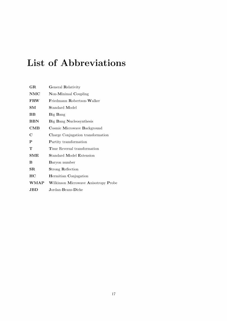
List of Abbreviations
GR General Relativity
NMC Non-Minimal Coupling
FRW Friedmann Robertson-Walker
SM Standard Model
BB Big Bang
BBN Big Bang Nucleosynthesis
CMB Cosmic Microwave Background
C Charge Conjugation transformation
P Partity transformation
T Time Reversal transformation
SME Standard Model Extension
B Baryon number
SR Strong Reflection
HC Hermitian Conjugation
WMAP Wilkinson Microwave Anisotropy Probe
JBD Jordan-Brans-Dicke
17


List of Symbols
η Baryon-to-photon ratio
ηS Baryon-to-entropy ratio
nB Net particle number
Γ Decay width
TF Freeze-out temperature
TD Decoupling temperature
g Degrees of freedom
g∗ Relativistic degrees of freedom
µ Chemical potential
ρ Energy density
p Pressure
n Particle Number
s Entropy density
Tµν Energy-momentum tensor
gµν Spacetime metric
R Ricci Scalar
Lm Matter Lagrangian density
The physical constants c, kB , ~ are usually set to 1.
The metric signature is (+ - - -).
19


Chapter 1
Introduction
One of the major mysteries of our Universe is that we do not observe the same number of particles and
antiparticles. In fact, the observed Universe is entirely made of matter, except for a tiny percentage of
antiparticles detected in the cosmic ray flux.
Starting from a neutral and symmetric Universe, we cannot explain this asymmetry. This is based
on the fact that every well-defined relativistic quantum field theory that we have constructed respects
CPT invariance, which — in turn — identifies every particle state with an antiparticle one.
Baryogenesis is a complicated problem, with many open questions, and the subject of intensive
research. It connects different areas of physics beyond elementary particle theory: on one hand, it
is constrained by cosmological parameters and the sequential phases of expansion; on the other hand,
quantum field theory is an obvious prerequisite to define the state of an antiparticle and to study effective
theories. Moreover, this problem requires various concepts of thermodynamics and, in particular, a
thermodynamic formulation applied to the early Universe, an important topic that we will discuss in this
work.
Sakharov (1967) proposed the three necessary conditions that should be required by all baryogen-
esis models. Since known mechanisms are not able to generate enough matter-antimatter asymmetry,
extensions of the Standard Model are required. We could have focused on reviewing the specific features
of each model and its particular problems — a nice review on these topics can be found, for example,
in Ref. [1] — ; instead, we chose to explore an alternative to the standard conditions, that allows us to
discuss the CPT invariance in a cosmological context.
In fact, faced with the consequences of the CPT theorem, a natural way to address the open question
of how an expanding Universe could develop an excess of baryons over antibaryons is to argue that CPT
might not have been already established in the primary stages of evolution. This allows for a different
particle-antiparticle interaction with the cosmological background, while ensuring the standard evolution
that leads to a CPT-invariant ground state.
1

Chapter 1. Introduction 2
Moreover, bringing modified gravity models to the discussion, we obtain modified field equations
that can enlarge the baryonic asymmetry to the observable amount, while enabling us to interpret ther-
modynamically the new conservation laws. In particular, entropy considerations might be altered, which
can significantly affect the cosmological parameter that characterizes this asymmetry.
The present mechanism for baryogenesis is an interesting framework to connect various sub-fields
of physics and to extend basic concepts of microphysics to the cosmological system. Aside from being
a rich problem to learn (not only the theory, but how this is compatible with observations and particle
experiments), this model allows us to complete and generalize previous work, hence contributing to a
deeper comprehension of gravitational baryogenesis.
This thesis is divided into four major parts:
1. The research topics, where Chapter 1 and Chapter 2 are included, regarding CPT invariance
and the thermal history of the Universe, where we review the status of observations leading to
the numerical value for the asymmetry parameter and the cosmological reasons for this to be the
baryon-to-entropy ratio;
2. The discussion of two existing models that incorporate CPT violation in an expanding
Universe, corresponding to spontaneous and gravitational baryogenesis. These models are studied
in Chapter 4 and Chapter 6, respectively;
3. The presentation, in Chapter 5, of the f(R)-model with the inclusion of a nonminimal geometry-
matter coupling (NMC) and the attractive features of the latter;
4. The new results, which are discussed also in Chapter 6, aiming to develop a model for the
generation of the baryon asymmetry, in the framework of modified gravity theories. This generalizes
previous works, where only the f(R)-function was included, and explores the impact of the NMC in
the mechanism leading to gravitational baryogenesis. This chapter is based upon the work reported
in Ref. [2].
At the beginning of each chapter, we describe — with more detail — the sequential line of thought
along this thesis.
Finally, in Chapter 7, we present our conclusions and prospects of future work.

Chapter 2
CPT Invariance
As the motivation for our work is a dynamical violation of CPT, we begin by exploring this invariance.
We derive a simple proof of the CPT theorem. This is a very interesting result and maybe the most
important one in what concerns the predictions of antiparticles. It states that a wide class of quantized
field theories is invariant with respect to the product of time reserval (T), charge conjugation (C) and
parity (P).
The aim of this proof is not to focus solely on mathematical techniques, but to discuss the physics
behind it. We will consider three types of fields - spin 0, spin 1/2 and spin 1. Given the generality of
the theorem, it is important to know where each assumption enters the proof to gain intuition on how it
could possibly be broken.
Later on, we justify several properties of particles/antiparticles that we will use in the course of the
work and which are consequence of the CPT Theorem. Finally, we address some questions regarding
CPT-violation phenomenology and experimental constraints.
2.1 Field Operators
Let us start by listing the equations for the various types of fields we will discuss.
Spin-0 fields are described by the Klein-Gordon equation:
(+m2)φ(x) = 0 , (+m2)φ∗(x) = 0 ; (2.1.1)
expanding the fields in terms of the creation and annihilation operators, we can derive the free field
commutation relations:
[φ(x), φ∗(y)] = i∆(x− y) , [φ(x), φ(y)] = [φ∗(x), φ∗(y)] = 0 . (2.1.2)
3

2.2. Discrete Symmetries 4
Spin-12 fields are described by the Dirac equation:
(i /∇−m)ψ(x) = 0 , ψ(x)(−i←−/∇ −m) = 0 ; (2.1.3)
similarly, the anticommutation relations read
ψα(x), ψβ(y) = i(i /∇+m)αβ∆(x− y) , ψα(x), ψβ(y) = ψα(x), ψβ(y) = 0 , (2.1.4)
where
ψ = ψ†γ0 , (2.1.5)
γµγν + γνγµ = 2gµν , (2.1.6)
with γ denoting the 4× 4 Dirac’s matrices. Since we are using the metric (+,-,-,-), it follows that
γ0† = γ0 , γi† = −γi (i = 1, 2, 3) . (2.1.7)
Spin-1 fields, in each component, also satisfy the Klein-Gordon equation:
(+m2)φµ(x) = 0 , (+m2)φ∗µ(x) = 0 ; (2.1.8)
whereas the commutation relations read
[φµ(x), φ∗ν(y)] = −i(gµν +
1
m2∂µ∂ν
)∆(x− y) , [φµ(x), φν(y)] = [φ∗µ(x), φ∗ν(y)] = 0 . (2.1.9)
For sake of simplicity, we used the same symbol m for all the masses appearing not only in the field
equations, but also in the commutator function.
The ∆ function is defined in appendix B and is calculated explicitly for the case of a spin-0 field.
The other cases can be found, for example, in Greiner’s Field Quantization [3]. The derivation of the
expression for ∆(x) will allow us to discuss its symmetry properties and consequently the invariance of
the transformed laws, subjected to the action of some symmetry operator.
2.2 Discrete Symmetries
If we want to understand the CPT Theorem, first we need to define each of these operations, which must
leave the field equations and commutation relations invariant.
2.2.1 Parity
To discuss parity, let us start by taking into account the existence of the improper Lorentz transformation
of space reflection:
x′ = −x , t′ = t . (2.2.10)

2.2. Discrete Symmetries 5
The corresponding transformation matrix is
Λµν =
1 0 0 0
0 −1 0 0
0 0 −1 0
0 0 0 −1
= gµν . (2.2.11)
In order to establish Lorentz covariance of the Dirac equation, we introduce a matrix such that
ψ′(x′) = ψ′(Λx) = S(Λ)ψ(x); then, after a Lorentz transformation, (2.1.3) remains invariant provided
an S can be found which has the property S(Λ)γµS−1(Λ)Λνµ = γν . Denoting S = P for the coordinate
reflection, this condition becomes
PγµP−1 = γµ , (2.2.12)
which is satisfied by
P = eiαγ0 . (2.2.13)
In spite of the arbitrariness in the choice of the phase factor, we have to be coherent in the choice of
the intrinsic parity of particles (for example, if we consider the exchange of pions between nucleons,
p+n→ π, which conserves parity, we need to guarantee that the intrinsic parity of the proton times the
intrinsic parity of the neutron equals the intrinsic parity of the pion). Generally, we define:
Pψ(r, t)P−1 = α′′P γ0ψ(−r, t) . (2.2.14)
Under this parity transformation, it is easy to show that the transformed field, ψ′(x) = α′′P γ0ψ(−r, t)
also satisfies the Dirac equation.
For the free Klein-Gordon theory, the condition
Pφ(r, t)P−1 = αPφ(−r, t) , (2.2.15)
satisfies
PL(r, t)P−1 = L(−r, t) . (2.2.16)
Moreover, if we include an electromagnetic current, that is, if we add to the Lagrangian density a
term representing the interaction, generally electromagnetic, of the quantum system with an external
field,
L → L− jµAµ , (2.2.17)
we can verify that (2.2.15) ensures
P jµ(r, t)P−1 = jµ(−r, t) , (2.2.18)
so the equations of motion remain unchanged. This is true because, working with the wave equation
(2.1.1), we were able to identify the conserved current with jµ = i(φ∗∇µφ − φ∇µφ∗). This parity
transformation also leaves the commutation relations invariant.

2.2. Discrete Symmetries 6
Finally, in the case of the spin-1 field, the spatial components transform as a vector under spatial
reflection, while the time component remains unaffected; thus
Pφi(r, t)P−1 = −α′Pφi(−r, t) , (2.2.19)
Pφ0(r, t)P−1 = α′Pφ0(−r, t) . (2.2.20)
2.2.2 Charge Conjugation
Now we focus on the charge conjugation operation, a symmetry that emerges from the fact that to each
particle, there is an antiparticle. In particular, it sustains the idea that the existence of electrons implies
the existence of positrons, which was a crucial aspect to understand the hole theory that emerged from
the negative solutions of the Dirac equation. To avoid these unphysical solutions, Dirac proposed that
the vacuum of the theory corresponds to a configuration where all negative energy states are occupied,
forming the so-called “Dirac sea”; positive energy electrons are then forbidden to fall into this fully
occupied state by Pauli’s Exclusion Principle. On the contrary, a photon could excite an electron from
a negative energy state, leaving a hole in the vacuum. The physical interpretation is that this hole
appearing in the absence of an energy −E (E > 0) and a charge equal to e (e < 0) is equivalent to the
presence of a positron with positive energy +E and charge −e. The modern version of this picture is
understood in terms of the Feynman-Stuckelberg interpretation. The point we wish to underline is that
there is a one-to-one (experimentally established) correspondence between the negative solutions of the
Dirac equation
(i /∇− e /A−m)ψ = 0 , (2.2.21)
and the positron wave function, ψc. Following this interpretation, positrons appear as positively charged
electrons, so ψc will be a positive-energy solution of the equation
(i /∇+ e /A−m)ψc = 0 . (2.2.22)
There should be a transformation which, starting with equation (2.2.21), would lead us to the
existence of an antiparticle satisfying equation (2.2.22). Taking the complex conjugate of the first, we
obtain
[(i∂µ + eAµ)γµ∗ +m]ψ∗ = 0 , (2.2.23)
with Aµ = A∗µ. If we can now find a nonsingular matrix, that we denote Cγ0, with the algebra
(Cγ0)γµ∗(Cγ0)−1 = −γµ , (2.2.24)
we will find the desired form
(i /∇+ e /A−m)(Cγ0ψ∗) = 0 , (2.2.25)
with
Cγ0ψ∗ = CψT
= ψc (2.2.26)

2.2. Discrete Symmetries 7
the positron wave function. We may verify that such a matrix C indeed exists by explicit construction.
In our representation (C.0.1 and C.0.2), γ0γµ∗γ0 = γµT , so that condition (2.2.24) becomes CγµTC−1 =
−γµ, or
C−1γµC = −γµT . (2.2.27)
In this representation, C must commute with γ1 and γ3 and anticommute with γ0 and γ2; this is easily
satisfied for
C = iγ2γ0 = −C−1 = −C† = −CT . (2.2.28)
It is enough to be able to construct a matrix C in any given representation; applying a unitary
transformation to any other one will give a matrix appropriate to the new representation. The definite
operation has the form
Cψ(r, t)C−1 = α′′CCψT, (2.2.29)
Cψ(r, t)C−1 = −α′′∗C ψTC† . (2.2.30)
There is a phase arbitrariness in our definitions, just like in the case of a parity transformation.
The operator (2.2.26) explicitly constructs the wave function of a positron. However, we would
like to develop from it an invariance operation for the Dirac equation. This is possible if the charge
conjugation transformation additionally changes the sign of the electromagnetic field. Then, the sequence
of instructions
1. take the complex conjugate ;
2. multiply by Cγ0 ;
3. replace Aµ by −Aµ ;
defines a formal symmetry operation of the Dirac theory. This means that, for each physically realizable
state containing an electron in a potential Aµ(x), there corresponds a physical realizable state of a positron
in a potential −Aµ(x). Although we already knew the equivalence of these two dynamics from classical
considerations, we are led to a new and surprising result: if there exist electrons of mass m and charge
e, there must also exist positrons of mass m and charge −e1.
When applying charge conjugation to the Lagrangian, in order to check its invariance, one encounters
the difficulty that products of operators are transformed into those of the Hermitian adjoints:
Cψ(x)γµψ(x)C−1 = −ψα(x)C−1αβ γ
µβλCλτψτ (x) = ψα(x)γµταψτ (x) . (2.2.31)
In order to make the transformed Lagrangian comparable with the original one, we need to assume
from the beginning that a process of proper symmetrization (or equivalently normal ordering) has been
1This conclusion is a consequence of the identification of (2.2.26) with the positron field. Later on, the state of an
antiparticle is generalized to be |ψ′〉 ≡ CPT |ψ〉, as charge conjugation can be violated and the consequences of the CPT
theorem hold still.

2.2. Discrete Symmetries 8
applied to it, so that all quantities are symmetrized in their boson fields and antisymmetrized in the
fermion fields. Identifying the electromagnetic current with
jµ(x) =1
2
[ψ(x), γµψ(x)
], (2.2.32)
it follows directly from (2.2.31) that Cjµ(x)C−1 = −jµ(x), and therefore this quantity is odd under
charge conjugation transformation, as it should: reversing the role of particle and antiparticle reverses
the electromagnetic field; then, the electromagnetic current must also gain a minus sign, in order to
preserve the invariance of the (Aµjµ) interaction.
We saved for last the transformation of boson fields. In terms of the Lagrangian (2.2.17), the previous
discussion leads to the requirement, for a theory which is charge conjugation invariant, that there exists
a unitary operator such that
CL(x)C−1 = L(x) , (2.2.33)
and
Cjµ(x)C−1 = −jµ(x) . (2.2.34)
Since L(x)→ L(x) and jµ(x)→ −jµ(x) under the transformation φ↔ φ∗, we search for a C which
has the property
Cφ(r, t)C−1 = αCφ∗(r, t) . (2.2.35)
Again, the generalization for spin-1 fields follows the same principles:
Cφµ(r, t)C−1 = α′Cφ∗µ(r, t) . (2.2.36)
Note, for completeness, that C must also change electrically neutral particles, described by non-
hermitian fields, such as the neutron (n), to their antiparticles (n), in order that the conservation laws of
strangeness, nucleon number and isospin are invariant under C. For hermitian fields, like those describing
photons, the commutation relations vanish and the particle is not distinguishable from the antiparticle;
under C, the hermitian field can at most change by a factor −1. As discussed, in the case of the
electromagnetic field, Aµ must transform according to:
CAµ(x)C−1 = −Aµ(x) , (2.2.37)
in order to leave the Lagrangian density invariant.
Conventionally, C |0〉 = + |0〉 is postulated, as well as P |0〉 = + |0〉, for the free field vacuum |0〉;
that means the vacuum is an even eigenstate. Also, for an n−photon state, the eigenvalue of C according
to (2.2.37) is (−1)n. This is important to understand the consistency of the phase in our definitions.
Consider, for example, the observation of the decay π0 → 2γ. If charge conjugation invariance holds in
strong and electromagnetic interactions, then π0 must be even under C if it evolves to the state of γγ,
which — by equation (2.2.37) — is even.

2.2. Discrete Symmetries 9
2.2.3 Time Reversal
If we transform the electron wave function under time reversal, we will obtain the original electron running
backwards in time. This state will be physically realizable, provided that the transformed wave function
ψ′ also satisfies the Dirac equation. Hence, we need to find an operator T which transforms physical
states evolving in time t to states as would be viewed on backwards, with t′ = −t.
To begin our discussion, consider the Heisenberg equation
[H, ψm(r, t)] = −i∂ψm(r, t)
∂t. (2.2.38)
If we seek a unitary operator U which leaves the action invariant and which transforms ψm(r, t) to
Wmnψn(r,−t) = Uψm(r, t)U−1, we obtain
[UHU−1, ψn(r, t′)] = i∂ψn(r, t′)
∂t′(2.2.39)
In order to restore equation (2.2.38), we would need U to transform H to −H. This is unacceptable
in physics, because it would mean that, after the transformation, the eigenvalues of H would be negative
relative to the vacuum state (the energy would be unbounded from below). To avoid this situation, T is
considered an antiunitary operator, that takes the complex conjugate of all c-numbers involved,
T iT−1 = −i . (2.2.40)
With this choice, (2.2.38) will be invariant under T . In terms of the Lagrangian density (2.2.17), the
theory will be time-reversal invariant if
TL(r, t)T−1 = L(r,−t) , (2.2.41)
and
T jµ(r, t)T−1 = jµ(r,−t) , (2.2.42)
meaning the electromagnetic currents are reversed while the charges are unchanged. Also, to guarantee
the invariance of the Lagrangian, Aµ should transform like:
Aµ(r, t)→ Aµ(r,−t) . (2.2.43)
In particular,−→A ′(t′) = −
−→A (t). Also,
−→∇ ′ =
−→∇ and −→x ′ = −→x . It is clear by now that the time-reversal
transformation changes i to −i; hence, T may be equivalent to taking the complex conjugate and then
multiplying by a 4× 4 constant matrix T :
ψ′(t′) = Tψ∗(t) . (2.2.44)
To construct the desired transformation, we consider the Dirac equation in the presence of an external
electromagnetic field2,
[(i∇µ − eAµ)γµ −m]ψ = 0 . (2.2.45)
2The coupling with the electromagnetic field is simply introduced by means of the substitution pµ → pµ − eAµ, where
pµ = i∇µ = i ∂∂xµ
and xµ = (t,−→x ).
2.2. Discrete Symmetries 10
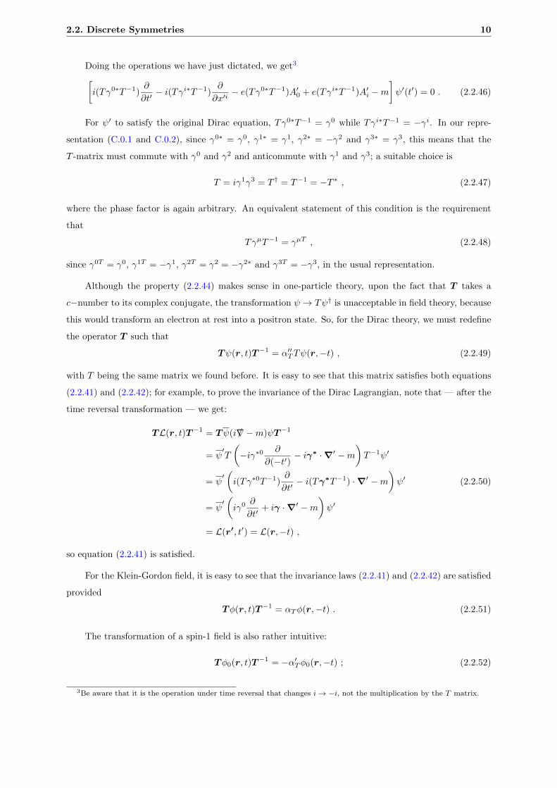
Doing the operations we have just dictated, we get3[i(Tγ0∗T−1)
∂
∂t′− i(Tγi∗T−1)
∂
∂x′i− e(Tγ0∗T−1)A′0 + e(Tγi∗T−1)A′i −m
]ψ′(t′) = 0 . (2.2.46)
For ψ′ to satisfy the original Dirac equation, Tγ0∗T−1 = γ0 while Tγi∗T−1 = −γi. In our repre-
sentation (C.0.1 and C.0.2), since γ0∗ = γ0, γ1∗ = γ1, γ2∗ = −γ2 and γ3∗ = γ3, this means that the
T -matrix must commute with γ0 and γ2 and anticommute with γ1 and γ3; a suitable choice is
T = iγ1γ3 = T † = T−1 = −T ∗ , (2.2.47)
where the phase factor is again arbitrary. An equivalent statement of this condition is the requirement
that
TγµT−1 = γµT , (2.2.48)
since γ0T = γ0, γ1T = −γ1, γ2T = γ2 = −γ2∗ and γ3T = −γ3, in the usual representation.
Although the property (2.2.44) makes sense in one-particle theory, upon the fact that T takes a
c−number to its complex conjugate, the transformation ψ → Tψ† is unacceptable in field theory, because
this would transform an electron at rest into a positron state. So, for the Dirac theory, we must redefine
the operator T such that
Tψ(r, t)T−1 = α′′TTψ(r,−t) , (2.2.49)
with T being the same matrix we found before. It is easy to see that this matrix satisfies both equations
(2.2.41) and (2.2.42); for example, to prove the invariance of the Dirac Lagrangian, note that — after the
time reversal transformation — we get:
TL(r, t)T−1 = Tψ(i /∇−m)ψT−1
= ψ′T
(−iγ∗0 ∂
∂(−t′)− iγ∗ ·∇′ −m
)T−1ψ′
= ψ′(i(Tγ∗0T−1)
∂
∂t′− i(Tγ∗T−1) ·∇′ −m
)ψ′
= ψ′(iγ0 ∂
∂t′+ iγ ·∇′ −m
)ψ′
= L(r′, t′) = L(r,−t) ,
(2.2.50)
so equation (2.2.41) is satisfied.
For the Klein-Gordon field, it is easy to see that the invariance laws (2.2.41) and (2.2.42) are satisfied
provided
Tφ(r, t)T−1 = αTφ(r,−t) . (2.2.51)
The transformation of a spin-1 field is also rather intuitive:
Tφ0(r, t)T−1 = −α′Tφ0(r,−t) ; (2.2.52)
3Be aware that it is the operation under time reversal that changes i→ −i, not the multiplication by the T matrix.

2.3. Proof of the CPT Theorem 11
Tφi(r, t)T−1 = α′Tφi(r,−t) . (2.2.53)
Let us now analyze the behavior of the various fields. The equations of motion of spin-zero and
spin-one fields are easily seen to be preserved. But recalling the symmetry properties of the ∆ function
(see appendix B), we notice it changes sign under the substitution t→ −t. Again, this only means that
T cannot be a linear operator. Since the r.h.s of the commutation relations are purely imaginary, it
suffices to define T as an antilinear operator, as argued when discussing the Heisenberg equation for the
evolution of fields.
Another important property to notice is that the modulus of the c-numbers, αU , α′U and α′′U with
U = C,P, T , must be equal to one, in order to conserve the commutation relations.
Note also that combining equations (2.2.27) and (2.2.48), we get the following result
(CT )γµ(CT )−1 = −γµ , (2.2.54)
which shows that, since γµ, γ5 = 0, we may put
CT = γ5 . (2.2.55)
2.3 Proof of the CPT Theorem
In 1957, Luders [4] proved that a wide class of field theories invariant under the proper Lorentz group
(the field operator expansion and the commutation relations are built to be Lorentz invariant) is also
invariant under the product CPT. This theorem does not state that this product is identical to the
unit operator, but that the c-numbers αT , αC , αP , etc., can be chosen in a way that one has invariance.
Luders proof, which we will follow up, consists on explicitly constructing an operation under which the
theory is invariant and then showing that this is equivalent to the product CPT. This operation is done
in two steps: the strong reflection and the subsequent hermitian conjugation.
2.3.1 Strong Reflection
Working out permutations of CPT on specific examples, we can convince ourselves that it is actually
quite difficult to construct a Hamiltonian that violates the product of C, P and T taken in any order
(with suitable choices of the phases)4. This fact induces us to think that there is something fundamental
about the product of these three symmetries. Then we are naturally led to ask what are the minimal
assumptions on a field theory of elementary particles, in order that this product is a good operation that
leaves it invariant. If we think about it, as a theoretical physicist that is faced with this symmetry hint, we
would start by assuming invariance under proper orthochronous Lorentz transformations, since all objects
4This idea is explored in the fifth chapter of Sakurai’s book [5], for example.

2.3. Proof of the CPT Theorem 12
in field theory (the operators itself, the field equations, the commutation relations and propagators, the
volume elements on integrals, etc.) are constructed to preserve the relativistic laws. As we go along, it
will become necessary to make a few more assumptions, like the usual spin-statistics connection.
Before considering the product CPT, let us enquire if there is any transformation such that the
transformation property depends only on the oddness or evenness of the rank (number of uncontracted
indexes) of a tensor density or some other quantity. That is, if there exists, for a tensor with n uncon-
tracted Lorentz indexes, any transformation that takes
Oµν...λσ(x)→ (−1)nOµν...λσ(−x) . (2.3.56)
If we can find a set of operations that lead to (2.3.56), then anything we can write down for an
interaction density will be accordingly invariant under that set of operations. This would be true for
both the Lagrangian density, which is a true scalar, and for the Hamiltonian density, which is the 0-0
component of the energy-momentum tensor, a symmetric tensor of rank 2. Note also that, for the 4-
current, transformation (2.3.56) means jµ(x)→ −jµ(−x), which cannot be brought by either C, P or T
alone. We now want to show that the desired set of operations called “strong reflection” exists and is
closely related to the product CPT (even though this is not the whole story).
We only assume Lorentz invariance — not reflection invariance under parity nor time reversal — so
that the rank of a tensor is defined exclusively from its behavior under the proper orthochronous Lorentz
transformations5, L↑+:
Oµν...λσ → Λµ′
µΛν′
ν ...Λλ′
λΛσ′
σOµ′ν′...λ′σ′ , (2.3.57)
where Λµ′
µ stands for the matrix element associated with the Lorentz transformation xµ → Λµ′
µxµ′ .
Now let us wonder what is the physical meaning of the transformation (2.3.56). If 4-dimensional
space were Euclidean, there would be only two classes of Lorentz transformations6 , one with detΛµν = 1
and the other one with detΛµν = −1. In particular, the transformation
x→ −x , Λµν =
−1 0
−1
−1
0 −1
(2.3.58)
is of the first type and can be generated by continuous rotations in 4-space: simply rotate in the 3 − 4
plane about the 1 − 2 plane by π and then rotate in the 1 − 2 plane about the 3 − 4 plane by π (here,
5The proper orthochronous Lorentz group is defined by the condition L↑+ = Λ ∈ L : detΛ = +1,Λ00 ≥ 1. This subgroup
is the one (out of four) component of the Lorentz group that contains all Lorentz transformations that can be connected to
the identity by a continuous curve lying in the group. It is generated by ordinary spatial rotations and Lorentz boosts. It
can be shown that if M denotes a general matrix (with ordinary group operations) with det(M) = 1, then Λ(M) ∈ L↑+.6For 4-dimensional Euclidean space, the metric becomes gµν = δµν ; hence, the condition on the Lorentz matrix, ΛT gΛ =
g, reduces to Λµ0Λµ0 = 1, which implies (Λ00)2 = 1 − (Λi0)2 ≤ 1 so that, for ordinary Lorentz transformations (Λ0
0,Λi0
reals), the usual two possible conditions on Λ00 reduce to one: −1 < (Λ0
0) < 1.

2.3. Proof of the CPT Theorem 13
the 4 direction corresponds to the direction of time, that now behaves as any other spatial component).
States with angular momentum J would transform as:
|ψ〉 → S |ψ〉 ,
S = eiJ12πeiJ34π ,(2.3.59)
where Jij are the generators of the rotation group. Recall that a general Lorentz transformation has the
form
Uω = eiωµν
2 Jµν , (2.3.60)
where ωµν are six independent parameters (three for boosts along each spatial direction and three for
a generic rotation). The generators Jµν include not only differential operators acting on the coordinate
functions (the orbital part), but also the operators acting on the spinors, so they are generally written as
Jµν = i(xν∂µ − xµ∂ν) +σµν2
. (2.3.61)
We know that a scalar function is invariant under rotations and that a vector transforms as φ′i(x) =
Rjiφj(R−1x); analogously, a solution of Dirac equation should transform as ψ′a(x) = Sbaψb(Λ
−1x), with
S satisfying the condition
S−1γµS = Λµνγν , (2.3.62)
to guarantee the covariance of the Dirac equation. Expanding (2.3.60) around the identity and using the
fact that ωµν = −ωνµ, yields
S(ω) = 1 +i
4ωµνσµν + ... (2.3.63)
and we can identify σµν/2 with the generators of the Lorentz group acting on the Dirac space. If we
now use this result on the condition (2.3.62), we get a relation between these generators and the gamma
matrices:
σµν =i
2[γµ, γν ] . (2.3.64)
Returning to our discussion, under the transformation (2.3.58), the field operators transform as
φ(x)→ φ(−x) ; (2.3.65)
φµ(x)→ −φµ(−x) ; (2.3.66)
ψ(x)→ eiπ2 σ12ei
π2 σ34ψ(−x) . (2.3.67)
The σij operators in the exponent of equation (2.3.67) are found to be (see complement C):
σ12 =
σ3 0
0 σ3
, σ34 = −i
0 σ3
σ3 0
. (2.3.68)
Neglecting the unimportant phase factor in σ34 and since σ23 = 1, we can expand the exponentials
in terms of sine and cosine functions:
ψ(x)→(
cosπ
2+ iσ12 sin
π
2
)(cos
π
2+ iσ34 sin
π
2
)ψ(−x) = γ5ψ(−x) . (2.3.69)

2.3. Proof of the CPT Theorem 14
In reality, however, the space is not Euclidean. The transformation x→ −x belongs to L↓+, because
Λ00 is negative and cannot be brought about continuously from the identity doing infinitesimal transfor-
mations. Even so, this gives a hint why the transformation ψ → γ5ψ(−x) (up to a phase) has something
to do with Oµν...λσ → (−1)nOµν...λσ. It turns out the situation is a little less simple, and this operation
has to be made in conjunction with another one. At this point, we define (as Luders) the behaviour of
the field operators under strong reflection as follows:
φ(r, t)→ φ(−r,−t), φ∗(r, t)→ φ∗(−r,−t) ; (2.3.70)
φµ(r, t)→ −φµ(−r,−t), φ∗µ(r, t)→ −φ∗µ(−r,−t) ; (2.3.71)
ψ(r, t)→ γ5ψ(−r,−t), ψ(r, t)→ −ψ(−r,−t)γ5 . (2.3.72)
The invariance of the field equations is easy to check. For example, the transformed Dirac equation
reads:
i∂
∂(−xµ)γµγ5ψ(−x) + γ5mψ(−x) = 0 . (2.3.73)
Multiplying by γ5 on the left and using that γµ, γ5 = 0 and γ25 = 1, we obtain the original Dirac
equation, which completes the proof. The invariance of the boson equations is trivial to check. However,
when analysing the commutation relations for bosons, we find that they are not invariant, since the right
hand side changes sign because ∆(x) is odd. When dealing with time reversal, we encountered a similar
situation. We solved it, taking advantage of the occurrence of the imaginary unit in the commutation
relations, and defined time reversal as an antilinear operator. Facing with this problem, Pauli postulated
that the strong reflection shall produce a mapping that reverses the order of factors in the operator
algebra. This does not affect the anticommutation relations of fermion fields.
Let us review our reasoning: we are seeking a transformation with the property (2.3.56), because
then anything we can write for an interaction density would be automatically invariant under that set
of operations. Now we will prove the CPT theorem in two steps: firstly, showing that a wide class of
field theories are invariant under strong reflection; secondly, proving that the product of C, P, T taking
in any order is identical to SR followed by Hermitian conjugation. We could convince ourselves that the
change of order in SR is indeed essential, by looking at the Heisenberg equation:
i[P0, f ] =∂f
∂x0, P0 =
∫d3xT00 , (2.3.74)
where Tµν is the energy-momentum tensor. Note that the time derivative changes sign, but the total
energy P0 should remain invariant. Hence, we must take [P0, f ]→ [f, P0] to preserve the original form.
The behaviour of boson fields
For densities constructed out of boson fields and derivatives (of finite order) of fields, we know that for
each index we get a minus sign under SR. Change of order is irrelevant since the boson fields commute.
In order to achieve the invariance we want, we need to postulate the usual connection between spin and

2.3. Proof of the CPT Theorem 15
statistics, so all bilinear forms of boson fields must be properly symmetrized according to Bose-Einstein
statistics just as the bilinear covariants made of spinors must be antisymmetrized. Thus, for combinations
of boson fields,
Oµν...λσ → (−1)nO(x)µν...λσ (2.3.75)
is satisfied. L and T00 are made up of these operators with indices contracted. With each contraction,
the rank decreases by 2; hence:
L(x)→ L(−x) , T00(x)→ T00(−x) , (2.3.76)
as we would like.
The behaviour of fermion fields
The behavior of bilinear covariants of spinors is less obvious. To study them, we have to look into the
transformations of scalars, vectors and tensors which can be formed by means of the γ-matrices. The
transformation (2.3.72) followed by a change in the order of factors is the same as
ψ2Ωψ1 → [(−ψ2γ5)Ω(γ5ψ1)]T = −ψT1 γ5TΩT γ5Tψ
T
2 , (2.3.77)
because changing the order of factors causes ψβOβαψα → ψαOβαψβ = ψα(OT )αβψβ = (ψOψ)T . Then,
the usual connection between spin and statistics leads to the correct transformation properties:
: −ψT1(γ5Ωγ5
)TψT
2 : = : ψ2γ5Ωγ5ψ1 : (2.3.78)
We were thus led to introduce this additional postulate: In the Lagrangian, all products are sym-
metrized with respect to Bose fields and antisymmetrized with respect to Fermi fields. A postulate of this
type was already required for the discussion of charge conjugation, so it naturally extends to the proof
of the theorem. In the case of Dirac fields, the prescription is ψαΓαβψβ → 1/2[ψαΓαβψβ − ψβΓαβψα
].
Hence, the two terms in equation (2.3.78) are equal. Here, Ω corresponds to the well-known combinations
of γ matrices that appear in the spin one-half operators that we observe: the scalar (S) combination —
Ω equal to the identity — which simply gives ψψ; the vector (V ) combination that appears in iψγµψ; the
tensor (T ) one, in the expression ψσµνψ; the axial-vector (A) combination of γ matrices, identified with
the term iψγµγ5ψ; and finally the pseudoscalar (P ) term, identified with iψγ5ψ. It is trivial to check
that
γ5Ωγ5 = (−1)nΩ , (2.3.79)
where n = even for S, T, P and n = odd for V,A. Combining the results, we get
ψ2Ωψ1 → (−1)nψ2Ωψ1 , (2.3.80)
under SR. Without the normal spin-statistics relation, the result would be just the opposite of what we
want.

2.3. Proof of the CPT Theorem 16
We conclude that both L and T00 are invariant under strong reflection whether they are made up of
boson fields, fermion fields or even combinations of the two, provided that the “normal” symmetrization
relations hold.
2.3.2 Hermitian Conjugation
Strong reflection is defined on the operator algebra, corresponding to a mapping of the operator algebra
into itself which reverses the order of factors in products, as legitimate mathematically as that which
preserves the order. However, SR cannot be applied on a Hilbert space. Therefore, it was necessary to
introduce a second mapping of the operator algebra into itself which also reverses products and which
also leaves the interaction densities invariant. The result of the consecutive application of both operations
is defined in a Hilbert space. This second operation can be identified with Hermitian conjugation (HC).
It follows that a Hermitian Hamiltonian should also be required for the validity of this proof. If we then
show that the consecutive application of both operations is equivalent to the product of C, P and T, we
prove the invariance of the theory.
For boson fields, if we first apply SR and afterwards Hermitian conjugation, we end up with:
φ(x)SR−−→ φ(−x)
HC−−→ φ†(−x) ; (2.3.81)
φµ(x)SR−−→ −φµ(−x)
HC−−→ −φ†µ(−x) . (2.3.82)
Similarly, operating with CPT:
φ(x)C−→ αCφ
†(x)P−→ αCα
∗Pφ†(−~x, t) T−→ α∗CαPα
∗Tφ†(−x) ; (2.3.83)
φµ(x)C−→ α′Cφ
†µ(x)
P−→ α′Cα′∗P
φ†0(−~x, t)
−φ†i (−~x, t)
T−→ α′∗Cα′Pα′∗T
−φ†0(−x) .
−φ†i (−x) .
(2.3.84)
The two results are equal for α∗CαPα∗T = 1 and α′∗Cα
′Pα′∗T = 1. For a different order of C, P, T
operations, the condition on the phase may be modified.
Now we study the Dirac fields. We have:
ψSR−−→ ψT γ5T HC−−→ γ5ψ†T = γ5T γ0T γ0Tψ†T = −γ0γ5ψ
T. (2.3.85)
While operating with CPT:
ψC−→ α′′CCψ
T P−→ α′′Cα′′∗P Cγ
0ψT
= −α′′Cα′′∗P γ0CψT T−→
α′′∗C α′′Pα′′∗T γ
0CTψT
= α′′∗C α′′Pα′′∗T γ
0γ5ψT. (2.3.86)
Thus, CPT and SR followed by HC give the same result if α′′∗C α′′Pα′′∗T = −1. The condition on the
phase is modified if C, P or T are applied in a different order. This completes the proof that a quantized

2.3. Proof of the CPT Theorem 17
field theory constructed from fields of spin 0, 1/2 and 1 is invariant with respect to the product CPT
taken in any order.
Our reasoning relied on the substitution of SR by an operator Θ (SR + HC) in Hilbert space (defined
because the order of operators is reversed by SR but restored by HC), which does not change the physical
observables. Then, under the combined operation, the theory remains invariant while its application is
meaningful for both the operator algebra and for the underlying Hilbert space. We completed the proof
demonstrating that Θ is indeed an antiunitary operator in Hilbert space: it is, up to a phase, identical
to the product of three operators in Hilbert space C, P and T. The first two are unitary, while time
reversal is antiunitary, hence Θ is an antiunitary operator. Note, finally, that the hermiticity of interaction
densities was not necessary for proving the invariance under SR, but to identify CPT-operation with SR
followed by HC.
2.3.3 Some comments on the proof
To prove the CPT Theorem, we followed the proof suggested by Luders, that clarifies the physical ideas
behind the successive application of these discrete symmetries, although it is not the most technical one,
neither it includes the generalization for higher spin fields (Pauli gave a general proof using the theory
of representations of the proper Lorentz group [6]).
We now summarize what we have assumed:
• Invariance under proper orthochronous Lorentz transformations;
• Interaction densities are local and constructed out of field operators and derivatives of field operators
of finite order;
• The normal connection between spin and statistics (with kinematically independent Dirac fields
anticommuting);
• Interaction densities are symmetrized and antisymmetrized in the proper way;
• The hermiticity of interaction densities.
Before continuing, we should realize the primary mathematical reasoning in what concerns discrete
symmetry operations: we have a quantum field theory, which is invariant under proper Lorentz transfor-
mations, and we ask for additional symmetry properties which may hold in the theory. One has to state
all the physical assumptions that the fields must satisfy, besides the transformation properties. So, before
formulating the CPT Theorem, it is necessary to make a mathematical formulation of the operations C,
P and T separately. At first sight, our task might consist on constructing all symmetry operations,
which are either unitary or antiunitary — as it is stated in Wigner’s Theorem — which transform the
field operators φr(x) into φr′(x′), with the spacetime coordinates being transformed by one of the four

2.4. Applications of the Theorem 18
discrete Lorentz transformations: Identity, Space Reflection, Time Reversal or Inversion of all four coor-
dinates. Having in mind the applications of these operations to interacting fields, we restrict our choices
to local-symmetry operations, requiring that φ′r(x′) is connected with φr(x) by a linear transformation
of the form:
φ′r′(x′) =
∑r
αr′rφr(x) . (2.3.87)
With the additional supposition of locality, it is shown [6] that the symmetry group is generated by
charge conjugation, space reflection and time-reversal.
2.4 Applications of the Theorem
Now, with the CPT Theorem in hand, we can deduce several interesting consequences for relativistic
quantum field theory, in what concerns the relation between particles and antiparticles. The latter must
exist, even if charge conjugation is not an exact symmetry of Nature. We focus on three predictions of
the Theorem that we will use recurrently in the course of this work: (1) mass equality; (2) opposite sign
of charge; and (3) equality of total decay widths of particle and antiparticle.
2.4.1 Mass equality
Consider a particle a at rest with the z-component of angular momentum m; then, applying the discrete
operations C,P, T in some (irrelevant) order, we have:
TPC |a,m〉 = TP |a,m〉 = T |a,m〉 = αTCP |a,−m〉 , (2.4.88)
where we have included a general (complex) phase, αCPT , which corresponds to a combination of the
phases that appear due to the successive application of each operation; a denotes the antiparticle. We
next write:
(mass)a = 〈a,m|H|a,m〉 = 〈a,m|(TCP )−1(TCP )|H|(TCP )−1(TCP )|a,m〉
= 〈a,−m|H|a,−m〉 = (mass)a ,(2.4.89)
where we have used the invariance of the Hamiltonian under CPT .
2.4.2 Opposite charges
If we apply each operation in CPT with no particular order, we conclude that the electromagnetic four-
current transforms as (CPT )jµ(x)(CPT )−1 = −jµ(−x). But jµ(x) = (ρ(x), j), where ρ is the charge
density; in particular, (CPT )ρ(x)(CPT )−1 = −ρ(−x). Consequently, we have:
Qa = 〈a| ∫ d3xρ(x)|a〉 = 〈a|(CPT )−1(CPT ) ∫ d3xρ(x)(CPT )−1(CPT )|a〉
= 〈a| ∫ d3x[−ρ(−x)]|a〉 = −Qa .(2.4.90)

2.4. Applications of the Theorem 19
2.4.3 Equality of Lifetimes
If CPT symmetry is valid, the scattering matrix S transforms under the antilinear CPT transformation
as [7]:
S → S ′ = (CPT )†S(CPT ) = S† . (2.4.91)
In the quantum theory of interactions, the scattering matrix defines the amplitudes for finding the
system — in the remote future — in the free7 final state |f〉, when it was prepared to be in the free initial
state |i〉 in the remote past, that is, Sfi ≡ 〈f(out)|i(in)〉. These states form two complete sets of basis in the
Hilbert space; or equivalently, S describes how a given ’in’ state is expanded in terms of the ’out’ states:
|i(in)〉 =∑Sfi |f(out)〉, where the sum is extended to all possible final states. From this, the unitarity of
the S matrix follows. In the interaction picture, the S operator is obtained as S ≡ U (I)(∞,−∞) where U
is the time evolution operator, defined through Heisenberg’s equation: as the transformed operator must
still satisfy the latter, in the new coordinates, it follows that (CPT )†U (I)(t, t0)(CPT ) = U I(−t,−t0); so
that the scattering matrix is transformed into S† = S−1, as ’in’ and ’out’ states are interchanged by the
time reversal operation.
It is also usual to define S in terms of the transition matrix T ,
Sfi = δfi − i(2π)δ(Ef − Ei)Tfi , (2.4.92)
for which a similar relation holds:
T → T ′ = (CPT )†T (CPT ) = T † . (2.4.93)
Given these brief considerations, one can consider the lifetime of a particle |a〉 which can decay into
states |f〉 due to the effect of interactions Hint:
Γa ≡ τ−1a ∝
∑f
| 〈f |T |a〉 |2 . (2.4.94)
Although a phase space factor is included in the calculation of the total decay width, as given by Fermi’s
Golden Rule, it is the same for particles and antiparticles, because of the equality of their masses. Hence,
the only concern is the transition matrix; for this∑f
| 〈f |T |a〉 |2 =∑f
〈a|T †|f〉 〈f |T |a〉 = 〈a|T †T |a〉 , (2.4.95)
due to the completeness of the sum over the final states. Using the results from CPT invariance (2.4.91),
we get:
〈a|T †T |a〉 = 〈a|(CPT )†T T †(CPT )|a〉 = 〈aPT |T T †|aPT 〉 = 〈aPT |T †T |aPT 〉 , (2.4.96)
7The so-called ’in’ and ’out’ states are eigenstates of the full Hamiltonian (H0 +Hint), which specify the particle content
at time t = −∞ and t = +∞, respectively (Hint → 0 for t±∞).

2.5. (Good) Limitations of the CPT Invariance 20
where the last operation T T † = T †T results from the unitary of S8.
We now insert a sum over a complete set of states, yielding:∑f
〈aPT |T †|f〉 〈f |T |aPT 〉 =∑f
〈f |T |aPT 〉∗ 〈f |T |aPT 〉 =∑f
| 〈f |T |aPT 〉 |2 . (2.4.97)
Since the decay width cannot depend on the spin orientation (which is the effect of PT ) due to
rotational invariance, the result follows:
Γa = Γa . (2.4.98)
From the proof it does not follow that the partial widths of various decay channels must be identical
for particles and antiparticles; this is not required by the CPT Theorem (as it is by the C or CP
symmetries9). The laws ma = ma and Γa = Γa, and thus the validity of the CPT Theorem, have been
checked experimentally with high precision. The most sensitive probe for this purpose is the neutral
K meson — the physics of this system is discussed in the second chapter of Baym’s book [8]. Since
the decays of K0 and its antiparticle K0 interfere (the physical particles are combinations of these two
states), an upper bound for the mass difference is obtained with exceedingly high precision [9]:
mK0 −mK0 < 4.0× 10⁻¹⁹ GeV . (2.4.99)
A typical result for the agreement of particle and antiparticle lifetimes has been obtained for muons [9]:∣∣∣∣τµ+ − τµ−τaverage
∣∣∣∣ < (2± 8)× 10−5 . (2.4.100)
2.5 (Good) Limitations of the CPT Invariance
As we have been discussing, while CPT invariance guarantees the equalities of particle and antiparticle
masses and total decay widths, it does not require the partial decay widths for particle and antiparticle
to be equal. This is of fundamental importance in what concerns the present baryon asymmetry of the
Universe.
Let us contextualize the various work concerning CPT symmetry. Between 1955 and 1957, Luders
and Pauli derived explicit proofs of the CPT Theorem [6], based essentially on the operation of strong
reflection (in the literature, the theorem is sometimes called the Luders-Pauli Theorem). In another
paper published in 1957, Luders and Zumino investigated what are the connections between properties
of particles and antiparticles that follow from the general CPT invariance [10]. The fact that it permits
unequal partial decay widths was emphasized by Okubo [11], in the same year. He investigated the two
8Using the unitarity of S = 1−iT , it follows that 1 = SS† = 1−iT+iT †+TT †. Similarly, 1 = S†S = 1+iT †−iT+T †T ;
thus, we conclude that TT † = T †T .9The processes i→ f and i→ f have the same transition amplitude if charge conjugation is a symmetry of the theory; the
same is true for i→ f and fT → iT if this applies to time reversal (or, in the case of spinless particles, Γ[i→ f ] = Γ[f → i])

2.6. CPT Violation in the Early Universe 21
decay modes of the Σ+ hyperon and the corresponding ones for its antiparticle:
Σ+ → p+ π0 ; (2.5.101)
Σ+ → n+ π+ ; (2.5.102)
Σ+ → p+ π0 ; (2.5.103)
Σ+ → n+ π− . (2.5.104)
As a result of the CPT Theorem, the total lifetimes of Σ+
and Σ+ are equal. However, comput-
ing the ratio between the relative frequency of the events (2.5.101) and (2.5.103), he found out it can
strongly deviate from unity, if charge conjugation or time reversal does not hold (as in the case of weak
interactions), meaning the branching ratios can be different for particle and antiparticle. Going back to
section 2.4.3, it should be obvious why the proof does not extend to partial decay widths: unlike CP,
CPT inverts the in and out states; so, the sum over a complete set of final states is crucial to obtain the
equality (2.4.98).
Suppose that the Σ+ flux is bigger than the Σ+
flux: this can produce p faster than p. CP violation
in the decay producing the hyperons can actually produce a charge asymmetry to get the Σ+ flux bigger
than the other. This leaves a hint that CPT can be satisfied, CP violated and a baryon asymmetry can
arise, if Σ+
and Σ+ are produced equally, p and p are produced equally, but Σ+
decays less in a mode
that produces p and Σ+ decays more in a mode that produces p.
Later on, Sakharov (1967) proposed the three necessary conditions for baryogenesis [12], building on
Okubo’s work.
2.6 CPT Violation in the Early Universe
The CPT Theorem has withstood numerous high-precision experimental tests, one of the sharpest quoted
by the Particle Data Group involving the kaon particle-antiparticle mass difference (2.4.99). Given this
experimental precision and since CPT Theorem holds generally for relativistic particle theories, any sign
of its violation would be the signature of unconventional physics. It is thus a field of interest to examine
possible theoretical mechanisms through which this invariance could be broken.
Obviously, an immediate possibility to test CPT-violating effects is to construct a theory disobeying
any of the assumptions that enter the theorem. Another approach is to go beyond the Standard Model
of Particle Physics, considering — for example — string theories. Without entering into details, we can
readily be convinced that the usual premises of the theorem (e.g. locality) might be altered considering
that strings are extended objects.

2.6. CPT Violation in the Early Universe 22
2.6.1 Spontaneous CPT Violation
Being Lorentz invariance one of the major axioms leading to the CPT Theorem, the relation between the
breakdown of these two symmetries has been widely discussed in the literature. Moreover, it has been
shown [13] that — in some string theories — CPT violation may, in fact, occur through a mechanism based
on the spontaneous breaking of Lorentz symmetry, which may lead to observable effects at the current
energy levels accessible for experiments. A natural way for this to occur is imagining that a higher-
dimensional action, which is Lorentz and CPT invariant, exists in Nature. Then, the higher-dimensional
Lorentz group would have to be spontaneously broken, in order to describe our four-dimensional world:
this could in principle induce spontaneous CPT breaking.
Spontaneous Lorentz violation can occur in string theory because interactions can trigger nonzero
expectation values for Lorentz-tensor fields — which do not appear in our renormalizable gauge theories
in four dimensions. But the mechanism of spontaneous symmetry violation is well established in various
fields, like Condensed Matter Physics and Particle Physics; it is also very attractive because the symme-
try is violated through non-trivial ground-state solutions, while the underlying dynamics of the system
remains invariant. For example, consider classical electrodynamics: the energy density associated to some
electromagnetic field configuration is V (−→E ,−→B ) = 1
2 (−→E 2 +
−→B 2). The ground state is usually identified
with the lowest-energy configuration of a system; in this case, this corresponds to the field-free one, so
the vacuum is empty.
Let us now think about the Higgs field, which is a scalar. According to the mechanism that explains
how particles gain mass, the Higgs potential is identified with V (φ) = (φ2 − λ2)2 where λ is a constant.
Again, the lowest possible field energy is zero. Now this requires, however, φ to be non-vanishing: φ2 = λ2.
It follows that the vacuum of a system containing a Higgs-type field is not empty, but instead contains the
constant scalar field φvac ≡ 〈φ〉 = λeiθ, which is called the vacuum expectation value (VEV) of the field.
Note that, after expanding around the VEV, quadratic terms on SM fields appear in the Lagrangian, so
they develop mass. This is the Higgs mechanism at work. Also, note that 〈φ〉 — being a scalar — does
not choose a preferred direction in spacetime.
Finally, we take a look at a vector field−→C , whose existence is not predicted within the framework
of the SM. In analogy with the Higgs case, we take the expression for the energy density to be V (−→C ) =
(−→C 2 − λ2)2. Just like in the previous examples, this requires a non-vanishing VEV:
−→C vac ≡ 〈
−→C 〉 =
−→λ .
In this case, however, the true vacuum state contains an intrinsic direction, violating rotation invariance
and thus Lorentz symmetry. Interactions leading to this type of phenomena can be found in the context
of strings. Alan Kostelecky was the main driver behind the effort to develop a conceptual framework and
procedure for treating spontaneous CPT and Lorentz violation [14]. It is assumed that underlying the
effective four-dimensional action is a complete fundamental theory based on conventional quantum physics
and that is CPT and Poincare invariant. The fundamental theory is assumed to undergo spontaneous
CPT and Lorentz breaking. We remark some of the ideas concerning this theoretical approach.

2.6. CPT Violation in the Early Universe 23
2.6.2 CPT Violation in String Theory
Spontaneous breaking of Lorentz symmetry can occur in a theory that contains certain types of interaction
among Lorentz tensor fields, if such interactions produce nontrivial VEVs.
In string theory, solutions exist in which scalar field components have a nonzero value. This can
lead to an effective action for tensor field components that would give a VEV to the latter. For example,
the bosonic section of string field theory [15] contains the three field interaction term AµAµφ, between
the scalar φ and the massless vector Aµ. It follows that if the scalar field acquires a VEV, this would
contribute in turn to a squared mass for Aµ. Hence, for the appropriate sign of 〈φ〉, Aµ could also
get a vacuum expectation value, breaking Lorentz invariance. As Aµ has one uncontracted index, the
low-effective interaction term Aµjµ is odd under CPT. In this framework, Aµ is viewed as a background
field permeating the spacetime vacuum. In a CPT transformed version of an experiment, this will not
change, but the generalized current will, leading to effective CPT violation, as well as Lorentz violation.
The behaviour of these expectation values as background fields will be explained further on. We remark
the importance of identifying CPT with the Strong Reflection operation, to recognize the CPT-violating
terms that could appear in the action.
2.6.3 Standard Model Extension
Starting from the conventional SM Lagrangian, Lorentz-breaking modifications L′ can be added in a
simple way:
LSME = LSM + L′ , (2.6.105)
where the subscript SME refers to the generalized theory designating the Standard Model Extension.
Then, spontaneous CPT violation arises from nonzero expectation values acquired by some Lorentz
tensor T . Any interaction that is part of a four-dimensional effective theory must have mass dimension
four. M is considered to be the scale of the high momenta, that is, the scale of unification, which is large
compared to the scale m of the effective theory. The expectation values 〈T 〉 of the tensors T are assumed
to be Lorentz and possibly CPT violating, so any terms that survive after the spontaneous symmetry
breaking and are contemplated in L′ must be suppressed by, at least, on power of m/M relative to the
scale of the effective theory. As an example, consider the schematic form of terms that can appear in the
fermionic sector of the low-energy limit of the underlying theory:
L′ ⊃ λ
Mk〈T 〉 · ψ(Γ)(i∂)kχ+ h.c. , (2.6.106)
where ψ, χ are fermion fields, λ is a dimensionless coupling constant and Γ some gamma-matrix structure.
The procedure extends to add to the Lagrangian all possible extra terms that can incorporate the effects
of spontaneous Lorentz and CPT breaking at the level of the SM. This set is restricted by allowing only
hermitian terms that preserve SU(3) × SU(2) × U(1) gauge invariance and power-counting renormaliz-
ability in the extended action. Following these requirements, a general Lorentz-violating extension of the

2.6. CPT Violation in the Early Universe 24
SM that includes both CPT-even and CPT-odd terms has been constructed [16].
Since, in this context, CPT violation arises from nonzero expectations of Lorentz tensors, Lorentz
invariance is necessarily spontaneously violated too. The converse is false: expectation values of Lorentz
tensors with an even number of indices preserve CPT. For example, for the case k = 0, there are two
possible types of CPT-violating bilinears:
L′a = aµψγµψ, L′b = bµψγ5γ
µψ (2.6.107)
where aµ, bµ are interpreted as effective couplings arising from the spontaneous symmetry breaking
which are invariant under CPT transformations. Being interpreted as background fields, these tensorial
coefficients cause the terms in (2.6.107) to break CPT (having one Lorentz-index). On the contrary, it is
clear why the bilinears involving σµν and γ5 separately do not break CPT invariance. For completeness,
we also write the most relevant terms appearing in the case k = 1:
L′c =1
2icαψ
←→∂αψ , L′d =
1
2dαψγ5←→∂αψ , L′e = ieαµνψσ
µν←→∂αψ , (2.6.108)
which, in turn, break CPT as well. Here A←→∂µB ≡ A∂µB − (∂µA)B. In all these expressions, the
quantities aµ, bµ, cα, dα and eαµν (which are real due to the presumed hermiticity of the underlying theory)
are combinations of tensor VEVs, coupling constants, mass parameters and coefficients arising from the
decomposition of Γ.
In this framework, the violation of CPT invariance gives rise to the possibility of Baryogenesis in the
early Universe, as reported in Ref. [17]. This is possible, identifying a chemical potential in the interaction
(2.6.106) and constraining the free parameters (the cutoff scale and the decoupling temperature) to give
rise to the observed baryon asymmetry.
2.6.4 Background Fields
Next, we want to understand how Lorentz invariance is broken by these type of terms. Not only the
effective theory, but also the underlying one are constructed to be explicitly Lorentz invariant. All the
interaction densities in (2.6.107) and (2.6.108) have contracted indexes, that is, they are coordinate
Lorentz scalars. By construction, the SME extension is thus invariant under rotations or boosts of an
observer’s inertial frame - these are called observer Lorentz transformations. They should be contrasted
with rotations or boosts of the localized fields in a fixed observer coordinate system, called particle Lorentz
transformations.
The distinction between observer and particle transformations is essential to understand the break-
down of CPT symmetry in the present model. The CPT-violating terms are interpreted as arising from
constant background fields, like aµ and bµ. These eight quantities (four components for each field) trans-
form as two 4-vectors under observer Lorentz transformations and as eight scalars under particle Lorentz
transformation, whereas they are coupled to currents that transform as 4-vectors under both types of

2.6. CPT Violation in the Early Universe 25
transformation. Hence, observer Lorentz symmetry is still an invariance of the model, but the particle
Lorentz group is broken.
As an example, to understand the role of the so-called background fields, consider the following
analogy [16]: an electron with momentum perpendicular to a uniform magnetic field moves in a circle.
Suppose that, in the same observer frame, we instantaneously increase the magnitude of the electron
velocity without changing its direction, causing the electron to move in a circle of larger radius. This
particle boost is an observable effect in that particular frame, but leaves the background field unaffected.
However, if instead we apply an observer boost perpendicular to the magnetic field, the electron no longer
moves in a circle. In the new inertial frame, this is viewed as an−→E ×
−→B drift. The background magnetic
field is thus transformed into a new electromagnetic field under observer boosts, but it is unchanged by
particle boosts. This scalar character of the background field under this type of Lorentz transformations
that change the physics in a fixed inertial frame is what defines a particle transformation.
In this model, the behavior of the expectation fields as backgrounds is a consequence of their origin
as nonzero VEVs of Lorentz tensors in the bare theory. They are a global feature of the effective model
and cannot arise from localized experimental conditions. The key aspect for generating Lorentz- (and
CPT-) violating terms while preserving observer Lorentz invariance (or coordinate independence) is the
spontaneous Lorentz breaking in an underlying fully Lorentz-invariant theory, like string theory. Since
observer Lorentz invariance constrains the physics under coordinate changes made by an external observer,
an underlying theory with this property cannot lose it through internal interactions such as those leading
to spontaneous Lorentz violation.
However, this presents an immediate consequence: measurements of the expectation coefficients
will give different results in different observer’s frames. For example, considering a particle-antiparticle
oscillating system, like the neutral meson system, a Lagrangian term as (2.6.107) would introduce a
correction of the form ∆Λ ≈ −→p · −→a , where −→p is the direction of the particle beam and ∆Λ is the
difference of the diagonal terms in the Hamiltonian of the system (which, if non-zero, directly breaks
CPT invariance). As the Earth rotates, the direction of the experiment changes because it is attached to
the Earth, thus leading to a possible observable effect [18].

Chapter 3
Thermal History
In this chapter, we briefly discuss the first minutes in the history of the Universe.
Since we will use observational parameters to restrict the variables of our model, we need to under-
stand what are the cosmological evidences for a non-vanishing asymmetry and which parameters that we
measure today can be used to fix it in the first stages of evolution.
Therefore, it is crucial to review also the basic dynamics of an expanding Universe at early times,
which will lead us to conclude that, providing the Universe is isentropic (as in General Relativity),
this asymmetry is deduced from the observed baryon-to-entropy ratio, ηS ∼ 10−10. This parameter
is determined by precise WMAP and Planck measurements of the CMB anisotropy spectrum and the
predictions for the light element abundances produced during Big Bang Nucleosynthesis, meaning that
Baryogenesis is strictly constrained by these values. We explore some important features relative to BBN,
namely the freeze-out of weak interactions, which sets the starting point for the formation of primordial
elements, and how these are sensitive to the high entropy of the Universe (ηS 1).
The high precision concordance of these two measurements (CMB+BBN) is one of the greatest
successes in Cosmology. Hence, we also explore this link, confronting observational data and showing
that the observed asymmetry cannot be explained in the framework of the SM.
All this leads to the conclusion that some mechanism must be in place in order to generate the
overabundance of baryons compared to antibaryons.
3.1 Standard Cosmology
The observed Universe is composed of three components, each dominating at different epochs in the
expansion history due to their different dilution rates. They are: cosmological constant Λ with a constant
energy density (although more complicated proposals abound [19]); radiation (diluted as a−4); and non-
relativistic matter with p ρ (diluted slower, as a−3). This means that radiation dominated the very
26

3.1. Standard Cosmology 27
early Universe; later on, heavy dark and baryonic matter became relevant; and finally — up to the present
moment — Λ has been governing the dynamics.
3.1.1 Basic Concepts in General Relativity
Cosmological dynamics follow from the Einstein equation,
Gµν ≡ Rµν −1
2gµνR = 8πGTµν , (3.1.1)
where Gµν is the Einstein tensor, Rµν is the Ricci tensor, R is the Ricci scalar, gµν is the metric,
G is Newton’s gravitational constant and Tµν is the stress-energy tensor (here we are neglecting the
cosmological constant).
Admitting the homogeneity and isotropy of space, Einstein equation is simplified with the Robertson-
Walker metric, which yields the line element written in comoving coordinates as
ds2 = dt2 − a2(t)dr2
1− kr2+ r2dΩ2 , (3.1.2)
where a(t) is the cosmic scale factor and k the curvature.
Matter is assumed to behave as a perfect fluid, with an energy-momentum tensor
Tµν = (p+ ρ)uµuν − pgµν , (3.1.3)
where ρ and p are the energy density and pressure of the fluid; and uµ is its four-velocity, normalized so
that uµuµ = 1.
In GR, the geometry of spacetime is determined by the metric tensor and the metric connection,
which defines the covariant derivative on the spacetime. The former is written in terms of the Christoffel
symbols:
Γσµν =1
2gσα(gµα,ν + gαν,µ − gµν,α) , (3.1.4)
which are the general form of a metric-compatible and torsion-free affine connection, in General Relativity.
This allows us to define the Riemann curvature tensor:
Rρσµν = Γρνσ,µ − Γρµσ,ν + ΓρµλΓλνσ − ΓρνλΓλµσ . (3.1.5)
From it, one defines the Ricci tensor, Rµν = Rρµρν , which, upon contraction with the metric, gives the
Ricci scalar, R = gµνRµν .
Ploughing through the amount of algebra required to calculate the non-zero components of the
connection, it is then straightforward to compute the Ricci scalar [20]:
R = −6
(a
a+a2
a2+
k
a2
). (3.1.6)
The µ = ν = 0 component of Einstein’s equation gives the Friedmann equation:
H2 =8πG
3ρ , (3.1.7)

3.1. Standard Cosmology 28
defining the Hubble parameter, H ≡ a/a. We set k = 0, according to strong evidence pointing towards
a flat Universe; this comes from the fact that the sum of the observed abundances — Ω = ρ/ρcrit ≡
3H20ρ/8πG, where H0 is the present value of the Hubble parameter — for each cosmological component
is remarkably close to unity.
Likewise, the µ = i, ν = j components yield
− 2
(a
a+a2
a2
)= 8πGp . (3.1.8)
The quantity Gµν is covariantly conserved in GR, Gµν;ν =0 (the proof relies on the Bianchi identities
for the Riemann tensor). This implies, using Einstein equation, that the energy momentum tensor (3.1.3)
is also covariantly conserved, reflecting energy and momentum conservation in an expanding Universe:
T 0ν;ν = T 0ν
,ν + Γ0ανT
αν + ΓνανT0α
= T 00,0 + Γ0
ijTij + Γν0νT
00
= ρ+ 3a
a(ρ+ p) = 0 .
(3.1.9)
The Friedmann equation (3.1.7) admits not only non-relativistic dust, but also other types of matter
and energy. In order to investigate how different fluids evolve in an expanding Universe, we can start by
considering the First Law of Thermodynamics,
dE = −pdV + TdS , (3.1.10)
where the variation of energy in a given volume is due to the work or heat transferred in and out of it.
If the expansion of the Universe was adiabatic, we would set TdS = 0. Then, for a fluid of energy
density ρ and pressure p enclosed in a comoving volume V = a3, we would have:
d(ρa3) = −pd(a3) . (3.1.11)
Differentiating with respect to time, one can write the equation above as a conservation law:
ρ = −3H(ρ+ p) . (3.1.12)
As this gives the same result as equation (3.1.9), our Universe can —indeed — be regarded as isentropic1.
Equation (3.1.12) also let us know the evolution of the energy density: for a simple equation of state,
p = ωρ, it evolves like ρ ∝ a−3(1+ω). Examples of interest include dust/ nonrelativistic matter (ω = 0,
so that ρm ∝ a−3), radiation (ω = 1/3, implying ρr ∝ a−4) and a cosmological constant (ω = −1, which
means pλ = −ρλ).
3.1.2 Expansion Rate, Decoupling of Species and Freeze-out
The key to understand the thermal history of the Universe is the comparison between the rate of inter-
actions Γ of the relevant processes and the rate of the expansion H. This can be done by looking at
1Note that we have assumed isentropy in the form of Tµν as a perfect fluid.

3.1. Standard Cosmology 29
the relevant terms in the equation describing the evolution of the particle number density, with a colli-
sion term taking into account the interactions with different particles. This corresponds to the general
Boltzmann equation:
ni + 3Hni = −〈σivi〉[n2i − (neq
i )2], (3.1.13)
where neqi denotes the equilibrium distribution of the particle species, σi is the total cross section of
processes that either destroy or create them, and vi is their interaction velocity. We can identify the
proportionality constant with the particle interaction rate,
Γ ≡ nσv . (3.1.14)
Then, equation (3.1.13) can be recast in the form
d lnNid ln a
= − Γ
H
[1−
(N eqi
Ni
)2], (3.1.15)
showing that any deviation from thermal equilibrium makes the system evolve towards thermal equilib-
rium once again. For example, starting with a deficit of particles, Ni N eqi , the r.h.s. gives a positive
contribution, making the number of particles grow until its equilibrium value. Similarly, if the number
of particles exceeds its equilibrium value, more particles will be destroyed until equilibrium is achieved.
When Γ H, the collision term dominates and the system quickly relaxes to a steady state with
particles assuming their equilibrium abundances. In other words, the timescale of particle interaction is
much smaller than the characteristic expansion time scale,
tC ≡1
Γ tH ≡
1
H, (3.1.16)
meaning that local equilibrium is reached before expansion becomes relevant. As the Universe cools,
however, interactions might not be able to keep up with the Hubble expansion (tH becomes larger): at
the critical time, tC ∼ tH , particles decouple from the thermal bath.
When Γ < H, the collision term cannot compensate for the Hubble expansion and the system departs
from thermal equilibrium. This implies that the abundance of the particle species i will remain constant
after the decoupling, which is known as freeze-out.
In the primitive Universe, for temperatures T 102 GeV, all the Standard Model (SM) particles
behaved as radiation, dominating the energy density of the Universe. We want to establish the magnitude
of the ratio Γ/H for scattering processes mediated by gauge bosons, which depends on whether they
are relativistic or non-relativistic at the decoupling time. Defining the generalized structure constant
α ≡ g2A/4π for the gauge coupling associated with a generic gauge boson A, we have2:
2In both limits, the cross section must be proportional to α2, since we are considering processes corresponding to diagrams
with two vertices involved. In the case of a massless boson, we cannot use the mass to describe the order of magnitude
of a typical cross section; instead, we use σ ∼ L2 ∼ T−2. In the case of a massive boson, the latter becomes (T/m)2, as
obtained rigorously in Sec. 3.5.

3.2. Equilibrium Thermodynamics 30
• For a massless boson, mA T , the cross section is σ ∝ α2
T 2 ;
• For a massive gauge boson3, mA & T , the typical cross section is σ ∼ G2AT
2, where GA ∼ α/m2A is
the generalized Fermi constant.
From dimensional analysis, Γ ∼ σT 3, as for relativistic particles v ∼ 1; while, from the Friedmann
equation (3.1.7), we get H ∼ T 2/mP , where mP = 1/√G is the Planck mass. Hence, the two conditions
above translate to (up to constant factors)
Γ
H∼
α2mP /T , for mA T
G2AmPT
3 , for mA & T .(3.1.17)
This means that a particle species can be in thermal equilibrium at high temperature, mA T
mP ; and decouple later on from the thermal bath, once the temperature drops below TD ∼ (G2AmP )−1/3 ∼
α−2/3(mA/mP )1/3mA . mA. For species which interact only through weak interactions (mW ∼ mZ ∼ 80
GeV, corresponding to GF ∼ 10−5 GeV−2), the decoupling temperature is near T ∼ 1 MeV.
If expansion had never overcome the interaction rates, the Universe would be filled with mostly
photons and equilibrium would make any other type of matter be destroyed at the same rate it is
created. Hence, it is crucial to understand the deviations from equilibrium that led to the freeze-out of
massive particles.
3.2 Equilibrium Thermodynamics
As we have seen, the SM predicts that, in the very early Universe, most particles were in thermal
equilibrium with photons — a thermal bath of particles. In order to describe this state and the subsequent
evolution, we need to review the basic properties of particle distributions in kinetic thermal equilibrium
[20]. For that, we use the familiar Bose-Einstein or Fermi-Dirac distributions which give to a system of
particles a level occupancy f , at a temperature T :
f(p) =1
eE−µT ± 1
, (3.2.18)
where E2 = |p|2 + m2 is the energy of particles; µ = (ρ + p)/n is the chemical potential; the (+) sign
corresponds to fermions, while the (−) refers to bosons. Local thermal equilibrium means not only kinetic
equilibrium, but also chemical equilibrium. Then if, for example, a species A interacts with species B, C
and D via scattering processes such as
A+B ←→ C +D , (3.2.19)
chemical equilibrium implies that µA + µB = µC + µD.
3Examples of these are W± or Z, the gauge bosons of the weak interaction, which receive masses below the scale of
electroweak symmetry breaking (T . 102 GeV).

3.2. Equilibrium Thermodynamics 31
Recalling statistical mechanics, we know that the density of states for a particle with g internal
degrees of freedom (e.g., spin) is g/(2π)3; in this way, we can compute the particle density in phase space
as the density of states times the distribution function. The phase space distribution allows us to evaluate
the associated number density n, energy density ρ and pressure p for our particle system:
n = g
∫d3p
(2π)3f(p) , (3.2.20)
ρ = g
∫d3p
(2π)3E(p)f(p) , (3.2.21)
p = g
∫d3p
(2π)3
|p|2
3E(p)f(p) . (3.2.22)
Next, we analyse the asymptotic limits of these expressions (assuming, for now, |µ| T ).
Relativistic species
For T m, the Bose-Einstein or Fermi-Dirac distribution becomes
f(y) =1
ey ± 1(3.2.23)
where y = |p|/T . This implies, for the particle number density,
n = g
∫ +∞
0
4π|p|2d|p|(2π)3
1
ey ± 1=
g
2π2T 3
∫ +∞
0
y2
ey ± 1dy . (3.2.24)
To evaluate integrals like this one, it is useful to consider the following results
1
ex + 1=
1
ex − 1− 2
e2x − 1; (3.2.25)
∫ +∞
0
yn
ey − 1dy = ζ(n+ 1)Γ(n+ 1) , (3.2.26)
where ζ(z) is the Riemann zeta-function.
For bosons, it is easy to obtain
nb =g
π2T 3ζ(3) . (3.2.27)
For fermions, we need to develop the integrand:
nf =g
2π2T 3
(∫ +∞
0
y2
ey − 1dy − 2
∫ +∞
0
y2
e2y − 1dy
)=
g
2π2T 3
(∫ +∞
0
y2
ey − 1dy − 1
4
∫ +∞
0
z2
ez − 1dz
)=
g
2π2T 3
(ζ(3)(2!)− 1
4ζ(3)(2!)
)=
3
4
g
π2ζ(3)T 3 ,
(3.2.28)
implying nf = (3/4)nb.
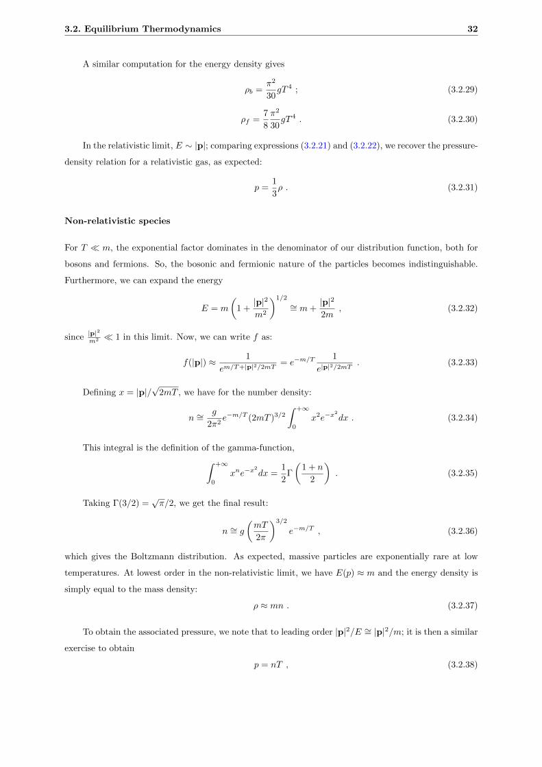
3.2. Equilibrium Thermodynamics 32
A similar computation for the energy density gives
ρb =π2
30gT 4 ; (3.2.29)
ρf =7
8
π2
30gT 4 . (3.2.30)
In the relativistic limit, E ∼ |p|; comparing expressions (3.2.21) and (3.2.22), we recover the pressure-
density relation for a relativistic gas, as expected:
p =1
3ρ . (3.2.31)
Non-relativistic species
For T m, the exponential factor dominates in the denominator of our distribution function, both for
bosons and fermions. So, the bosonic and fermionic nature of the particles becomes indistinguishable.
Furthermore, we can expand the energy
E = m
(1 +|p|2
m2
)1/2
∼= m+|p|2
2m, (3.2.32)
since |p|2
m2 1 in this limit. Now, we can write f as:
f(|p|) ≈ 1
em/T+|p|2/2mT = e−m/T1
e|p|2/2mT. (3.2.33)
Defining x = |p|/√
2mT , we have for the number density:
n ∼=g
2π2e−m/T (2mT )3/2
∫ +∞
0
x2e−x2
dx . (3.2.34)
This integral is the definition of the gamma-function,∫ +∞
0
xne−x2
dx =1
2Γ
(1 + n
2
). (3.2.35)
Taking Γ(3/2) =√π/2, we get the final result:
n ∼= g
(mT
2π
)3/2
e−m/T , (3.2.36)
which gives the Boltzmann distribution. As expected, massive particles are exponentially rare at low
temperatures. At lowest order in the non-relativistic limit, we have E(p) ≈ m and the energy density is
simply equal to the mass density:
ρ ≈ mn . (3.2.37)
To obtain the associated pressure, we note that to leading order |p|2/E ∼= |p|2/m; it is then a similar
exercise to obtain
p = nT , (3.2.38)

3.2. Equilibrium Thermodynamics 33
which corresponds to the familiar result for a non-relativistic perfect gas (the Boltzmann constant kB is
hidden in our system of units). Moreover, since T m, we have p ρ, showing that a non-relativistic
gas of particles acts like pressureless dust (i.e. matter).
By comparing the relativistic and the non-relativistic limits, we conclude that the three statistical
quantities — number density, energy density and pressure — fall exponentially (with the Boltzmann
factor) as the temperature drops below the particle’s mass. Again, this means that if equilibrium had
persisted until today, any massive particle species would be eventually suppressed and the Universe would
be mostly photons.
3.2.1 The Net Particle Number
Before continuing, it is important to restore a finite chemical potential in order to calculate the net
particle number; otherwise, the numbers of particles and antiparticles are equal.
Consider, for example, particle-antiparticle annihilation, X+ X ↔ γ+γ. We know that the number
of photons is not conserved at high temperatures, implying µγ = 0 (for instance, double Compton
scattering, e− + γ ↔ e− + γ + γ is effective at redshifts above z ∼= 2× 10⁶ [21]). This means that, if the
chemical potential of particle X is µX , then the chemical potential of the corresponding antiparticle X is
µX = −µX . (3.2.39)
Let us recalculate the relativistic limit for the particle number density of fermions, with µ 6= 0 and
T m. We obtain:
n− n =g
2π2
∫ ∞0
p2
(1
e(p−µ)/T + 1− 1
e(p+µ)/T + 1
)dp =
gT 3
6π2
[π2(µT
)+(µT
)3], (3.2.40)
with g denoting the number of intrinsic degrees of freedom of baryons.
Restoring a finite µ in the non-relativistic limit, we get:
n = g
(mT
2π
)3/2
e−(m−µ)/T , (3.2.41)
so that
n− n = 2g
(mT
2π
)3/2
e−m/T sinh(µT
). (3.2.42)
3.2.2 Energy and Entropy Density
Let T be the temperature of the photon gas in the early Universe. The total radiation density is the sum
over the energy densities of all relativistic species; hence
ρr =π2
30g?(T )T 4 , (3.2.43)
where g?(T ) counts the total number of effectively massless degrees of freedom of the plasma:

3.2. Equilibrium Thermodynamics 34
Figure 3.1: Variation of the number of relativistic degrees of freedom, g∗ and g∗S , with temperature
according to the Standard Model of Particle Physics [21].
g? =∑bosons
gi
(TiT
)4
+7
8
∑fermions
gi
(TiT
)4
. (3.2.44)
Here Ti denotes the effective temperature for any species i. There are two different contributions for
this sum: relativistic species in thermal equilibrium with the photons, with Ti = T mi; and relativistic
species that are not in thermal equilibrium with the photons (decoupled from the thermal bath), for
which Ti 6= T mi. For temperatures T & 102 GeV, all the degrees of freedom of the Standard Model
of Particle Physics are in equilibrium, corresponding to g? ≈ 107.
To describe the evolution of the Universe, it is useful to track a conserved quantity: Entropy, as
derived in section (3.1.1) from the energy-momentum conservation. To derive an expression for the
entropy, we once again resort to the First Law of Thermodynamics (for zero chemical potential):
TdS = dE + pdV . (3.2.45)
Considering S = S(V, T ) and E = E(V, T ) and using the fact that both the energy and the entropy
are extensive quantities (so we can replace the partial derivatives by the quantity itself), we get
T∂S
∂VdV + T
∂S
∂TdT − pdV =
∂E
∂VdV +
∂E
∂TdT ⇒
(TS
V− p)dV + T
∂S
∂TdT =
E
VdV +
∂E
∂TdT . (3.2.46)
Equating the terms in dV and dT , this yields:
∂E
∂T= T
∂S
∂T; (3.2.47)
E
V= T
S
V− p . (3.2.48)
From the second equality, we obtain:
s =ρ+ p
T, (3.2.49)
defining the entropy density as s = S/V . For radiation, with pi = ρi/3, this reduces to:
si =4
3
ρiTi
. (3.2.50)
3.2. Equilibrium Thermodynamics 35
Summing over all relativistic species, we can use the result (3.2.43) to write the total entropy density
of radiation in the early Universe:
s =2π2
45g?S(T )T 3 , (3.2.51)
where g?S(T ) is the effective number of relativistic degrees of freedom contributing to the entropy. Given
that si ∝ T 3i , this corresponds to
g?S =∑bosons
gi
(TiT
)3
+7
8
∑fermions
gi
(TiT
)3
. (3.2.52)
For species in thermal equilibrium, g?S = g?, which is not true for decoupled species. For most of
the history of the Universe, however, we can safely use the equality. The difference between these values
becomes significant only at low temperatures (see figure 3.1), as neutrinos decouple from the thermal
bath.
Entropy conservation implies that S = a3s remains constant as the Universe expands, hence
g?ST3a3 = const. (3.2.53)
Away from particle mass thresholds, g?S is approximately constant and T ∝ a−1, as expected for
relativistic particles (ρ ∝ a−4 ∝ T 4). Also, since s ∝ a−3, we can define the number of particles of a
given species in a comoving volume as:
Ni ≡ a3ni =nis, (3.2.54)
where we have redefined the scale factor to absorb constant factors. If no particles are being created or
destroyed in that volume, this quantity remains constant.
Using the previous results for the number density of particles in both the relativistic and non-
relativistic limits, we can write:
Ni =
45ζ(3)
2π4gig?S
, for T mi ;
454√
2π
gig?S
(miT
)3/2e−mi/T , for T mi .
(3.2.55)
For T mi, the conservation of this quantity is obvious: in the primitive thermal soup, all reactions
occur in both ways, so the particles which are produced get destroyed almost instantly. In the case of
T mi, the number of particles is not fixed until the temperature drops to the value at which reactions
which create/destroy them freeze out.
An important consequence of this is that, in the absence of interactions that produce or destroy
baryon number, the baryon-to-entropy ratio is conserved:
ηS =nBs
=nb − nb
s= const. (3.2.56)
where b and b denote baryons and antibaryons, respectively.
Before we discuss the next topic, it is convenient to write the Friedmann equation in the radiation
dominated era (t . 4× 10¹⁰ sec), for which the scale factor evolves as a(t) ∝ t1/2. Substituting (3.2.43)

3.3. The Matter-Antimatter Asymmetry 36
in (3.1.7), we obtain:
H =π√90
√g?T 2
MP, (3.2.57)
where we have defined the reduced Planck mass MP = 1/√
8πG ≈ 2.4 × 10¹⁸ GeV. Using the fact that
H = (1/2t), it is a trivial exercise to relate time and temperature:
t ≈(
T
MeV
)−2
sec . (3.2.58)
3.3 The Matter-Antimatter Asymmetry
3.3.1 Evidence for a Baryon Asymmetry
From the discussion of the second chapter, we conclude that CPT invariance ensures the baryon and
antibaryon thermal distributions to be equal. This is true, because they have equal masses and the
chemical potential can be neglected for most of the thermal history of the Universe (as we will investigate
in the next chapters, this is due to the smallness of the baryon-to-photon ratio). This means that if
annihilations are efficient in the early Universe (particles and antiparticles quickly annihilate via processes
like pp → γγ) and we start with equal amounts of matter and antimatter (the primitive Universe is
neutral), then there would be very few matter in the Universe, which would contain mainly radiation.
The observed Universe, however, is drastically different. We do not observe any bodies of antimatter
within the Solar System and, at the same time, cosmological traces of antibaryons are only found in
the cosmic ray data. As shown in figure 3.2, the measurements by the Alpha Magnetic Spectrometer
(AMS-02), a high energy particle detector designed to study the origin and nature of the cosmic rays up
to a few TeV from space — which was installed in the International Space Station in 2011 — and other
collaborations yield a flux of antiprotons p of about
npnp∼ 10−4 . (3.3.59)
We might wonder if the dominance of matter over antimatter is only local, with other regions of the
Universe having an opposite abundance and giving an overall symmetric Universe. If this were the case,
in the boundary between regions with opposite overabundance, annihilations of matter and antimatter
would originate an enormous flux that has not been observed (the energetic γ-rays, coming from the
decay of pp into π-mesons and followed by the decay π0 → 2γ).
For these reasons, it is widely accepted that — at least — the observable part of our Universe must
have developed an excess of particles over antiparticles, at some point in the cosmological evolution.
Moreover, we can conclude from observations that, if domains of matter and antimatter exist in the
Universe, they are separated by scales certainly larger than the radius of our galaxy (∼ 3 Kpc) and most
probably larger than the Virgo cluster (∼ 10 Mpc ) [24], with sophisticated γ-ray detectors potentially
capable of reaching a much more severe bound on the observational scale. A numerical analysis of this

3.3. The Matter-Antimatter Asymmetry 37
(a) Antiproton flux. (b) The average proton flux, for comparison.
Figure 3.2: Antiproton cosmic ray flux as measured by AMS-02 and other experimental collaborations.
The observed antiproton flux is consistent with secondary production due to collisions of baryons, leptons
or photons in the interstellar medium (taken from Refs. [22,23]).
problem was performed by Cohen, Rujula and Glashow (1997), showing that the Universe must consist
entirely of matter on all scales up to the Hubble size [25].
General considerations on Nucleosynthesis and the Baryon Number
The baryon number density nb does not remain constant during the evolution of the Universe; instead, it
scales like a−3, where a is the cosmological scale factor4. As the photon number density also scales like
this (use the result 3.2.53 in equation 3.2.27), one has another good way to define the baryon asymmetry
of the Universe, in terms of the quantity
η ≡ nBnγ
, (3.3.60)
where nB = nb − nb is the difference between the number of baryons and antibaryons per volume and
nγ = 2 ζ(3)π2 T
3 is the photon number density at some temperature.
The parameter η is essential for determining the present cosmological abundances of light elements
(such as H, D, 3He, 4He and 7Li) produced at the Big Bang Nucleosynthesis (BBN) era; and can be used
to estimate ηS which has been constant since then, because the Universe is isentropic. This is not quite
true for η, which is only constant away from particle mass thresholds (interchanging the entropy density
with the photon number, we carry an important g∗S factor, which shows variations of about two orders
of magnitude). It is important to discuss this in more detail, because several authors use either η or ηS
in phenomenological models for the generation of the baryon asymmetry, without explaining with clarity
the difference between the two.
It is true that NB is preserved once baryon-violating interaction freeze out. This is almost true for
4We argued that if no particles are created or destroyed in a comoving volume, then Ni = a3ni is constant.

3.3. The Matter-Antimatter Asymmetry 38
the number of photons, except for some additional ones created during the electron-positron annihilation
phase, at T ≈ 1 MeV, or in the course of stellar evolution. If this variation can be neglected — in the
absence of any significant, subsequent annihilations and providing most stellar photons are absorbed by
the intergalactic medium — η is approximately constant.
Observational probes strictly constrain the present value of η. This allows us to infer the baryon-to-
entropy ratio. The entropy is presently about equally divided between the 2.7 K photons and the three
cosmic neutrino backgrounds (with flavours e, µ, τ). Then, the present values for the entropy density and
the photon number density are the same up to a constant,
ηS =(nγs
)η =
45ζ(3)
g∗Sπ4η ≈ 10−1 × η , (3.3.61)
where we have used g∗S ≈ 2 + 7×68
(T νD
TCMB
)4
, T νD ∼ 2 MeV being the temperature at which neutrinos
decouple from the thermal bath [20]. If we want to map this present value back to the time the baryon-
violating forces decoupled from the thermal bath, we should rigorously use ηS .
Observations
The baryon-to-photon ratio is particularly constrained by BBN. The theoretical predictions and experi-
mental measurements are summarized in figure 3.3. The boxes represent the regions which are consistent
with experimental measurements, with their associated statistical and systematic uncertainties. The
4He curve is very sensitive to the uncertainty in the neutron lifetime (as discussed in the next section);
while the spreads in the curves for D, 3He and 7Li correspond to uncertainties in nuclear cross sections
estimated by computational methods [9]. There is acceptable agreement among the abundances when
5.8× 10⁻¹⁰ ≤ ηBBN ≤ 6.6× 10⁻¹⁰ (95% C.L.) . (3.3.62)
It might seem uninteresting to worry about numerical values besides the order of magnitude. It is
true that the latter suffices to discard statistical fluctuations as the origin of the asymmetry or to quantify
the incompatibility with the SM. However, this precision is one of the greatest agreements in Cosmology;
also, it turns out that the parameter space of our model using f(R)-theories is very sensitive to these
numerical factors.
While the η ranges spanned by the boxes in figure 3.3 do not all overlap, they are all within a factor
∼ 2 of each other. The lithium abundance corresponds to η values which are inconsistent with that
of the deuterium abundance, as well as the less constraining 4He abundance. This discrepancy could
simply reflect difficulty in determining the primordial lithium abundance; or it could hint towards new
physics, which can be a modification of the cosmological evolution that alters the lithium abundance but
not the other mass fractions. Despite this “lithium problem”, the overall concordance is remarkable; the
concordant η range (3.3.62) is essentially that implied by the D-mass fraction.
An independent way of measuring the baryon asymmetry is following up the Cosmic Microwave
Background. In spite of its 2.7 K uniformity, there are tiny fluctuations (apart from an anisotropy due

3.3. The Matter-Antimatter Asymmetry 39
Figure 3.3: The abundances of 4He, D, 3He and 7Li as predicted by the Standard Model of BBN. The
bands show the 95% C.L. range. Boxes indicate the observed light element abundances. The narrow
vertical band indicates the CMB measure of the cosmic baryon density, while the wider band indicates
the BBN concordance range (both at 95% C.L.) [9].

3.3. The Matter-Antimatter Asymmetry 40
to our motion relative to the CMB frame) within the CMB — of 1 part in 105 — that are sensible
to the matter density distribution at the time of last scattering; hence, they constrain η. WMAP has
been collecting data since 2001 to get more precise measurements of these anisotropies; in particular, the
Nine-Year Observations fixed the combination Ωbh2 = 0.02264±0.00050, where h is a conventionally used
parameter defined by h ≡ H0/100, H0 = 70.0± 2.2 kms−1Mpc−1. This fixes the baryon-to-photon ratio,
η ≡ nB/nγ , since the present photon number is calculated for T = TCMB and nB = ρB/mH = ΩBρC/mH ,
where ρB is the baryonic energy density, expressed in terms of the baryonic fraction of the critical density,
ρC ≡ (3H20 )/8πG. In the end, we get the final constraint from the CMB [26,27]:
ηCMB = (6.19± 0.14)× 10−10 . (3.3.63)
The concordance between this estimate and the BBN predictions is evident in figure 3.3; these obser-
vations are combined from diverse cosmological environments and it is remarkable that two independent
tests (the abundances of the light elements and the amplitudes of the acoustic peaks in the CMB angular
power spectrum) allow us to compare two measurements of η using very different physics at two widely
separated epochs. This allows us to compute the baryon-to-entropy ratio with precision [28]:
ηobsS ≡ nB
s. 9× 10⁻¹¹ . (3.3.64)
In Standard Cosmology, there is no change in the ηS value, after baryon-antibaryon b, b annihilations
freeze-out, and practically no change in η between BBN and CMB decoupling; thus, the agreement
between ηBBN and ηCMB is a key test. We have succeeded in the task of extrapolating our laws of physics
to an age of ∼ 1 sec of the Universe.
3.3.2 The Tragedy of a Symmetric Universe
Although the matter-antimatter asymmetry appears to be very large today, in the sense that nB ≈
nb nb, the fact that nB/s ≈ 10−10 implies that this asymmetry was once tiny: nB nb. To
see this, we assume for simplicity that nucleons are the fundamental baryons. Earlier than 10−6 sec
after the BB, temperature was higher than the mass of the nucleon (see equation 3.2.58); thus, nN ≈
nN ≈ nγ . The entropy density is s ∼ g∗nγ ≈ 102nN . In turn, the constancy of ηS ∼ 10−10 requires
(nN − nN )/nN ≈ 102nB/s ∼ O(10−8). This means that, during its earliest phase, the Universe was
nearly baryon symmetric.
Suppose we start with η = 0 (or nN = nN ). We can compute the final number of nucleons that are left
over, after annihilations have frozen out. Earlier than 10−6 sec after the BB, nucleons and antinucleons
were about as abundant as photons. At temperatures T . 1 GeV, the equilibrium abundance (as the
temperature falls below mb but the species are still coupled to the primordial plasma) of nucleons and
antinucleons isnNnγ
=nNnγ≈ gN
2.4
(2π)1/2
4
(mN
T
)3/2
e−mN/T . (3.3.65)

3.3. The Matter-Antimatter Asymmetry 41
When the Universe cools off, the number of nucleons (antinucleons) decreases as long as the anni-
hilation rate Γann ≈ nb 〈σv〉ann is larger than the expansion of the Universe. The thermally averaged
annihilation cross section 〈σv〉ann is of the order of 1/m2π with v ∼ 1 and where mπ is the pion mass.
The freeze-out temperature TF is obtained by setting Γ ≈ H, where the expansion rate of the Universe
is given by the Hubble parameter during radiation era, H ≈ 1.66√g∗T
2/mP ; then, we should solve
gN1
(2π)3/2x1/2e−x
mN
m2π
= 1.66g
1/2∗
mP
⇒ x−1/2ex ∼ 8
3(1.66)
1
(2π)3/2
mN
m2π
mP ≈ 6× 10¹⁹ ,
(3.3.66)
where we defined x = mN/T . Solving numerically, this gives xF ∼ 47(8); thus, TF ≈ 20 MeV. We
used gb = 8 considering the 4 spin states of the nucleon (n, p) system (×2 taking into account the
antiparticles) and O(g∗) ∼ 10 for T . 1 GeV5. At Tf ≈ 20 MeV, annihilations thus freeze out, nucleons
and antinucleons being so rare that they cannot annihilate any longer. Residual nucleon and antinucleon
to photon ratio can be calculated using equation (3.3.65):
nbnγ≈ (2π)1/2x
3/2F e−xF ∼ 10−18 , (3.3.67)
which is much smaller than the value required by Nucleosynthesis (the observed η parameter).
In order to avoid the annihilation catastrophe, we may suppose the existence of some mechanism that
separated matter from antimatter before T ≈ 32 MeV, which is the solution of equation (3.3.67) with
η ≈ 10−10. This value of temperature corresponds roughly to t ≈ 10−3 sec. Causality, however, excludes
this argument: during the radiation era, the scale factor evolves as a ∝ t1/2; then we can estimate the
size of the region causally connected at this time6, dradH (t) = 2t, obtaining a causal region way too small
to explain the asymmetry over the galaxy scales. If we take into account inflation, the region of the
Universe connected today was connected even at those early times. But, if the processes responsible for
the separation of matter from antimatter happened before inflation, then the baryon number would be
diluted by an enormous factor; on the contrary, if they happened after, there is no mechanism providing
a straightforward way to eliminate the boundaries between matter and antimatter islands.
Attempts to explain the same problem considering statistical (Poisson) fluctuations in the baryon
and antibaryon distributions have also failed. To see this, let us estimate how many baryons and photons
there are today in the volume that encompasses our galaxy. We consider the sun to be a typical star,
with an average density equal to ρ ≈ 1 g/cm3 and volume V = 1018 km3. Then, there are ≈
(ρ/mb)V ∼ 1057 baryons in a typical star. Since there are ≈ 1012 stars in a typical galaxy, our galaxy
contains ≈ 1069 baryons; and - using the observed η value - 1079 photons. At temperatures T & 1 GeV,
5At about this temperature, T ∼ 200 MeV, the quarks combine into baryons (protons, neutrons, ...) and mesons (pions,
...); only after this stage of evolution, we can talk about composite particles. Above the QCD phase transition, however,
almost all these particles (except the pions) are non-relativistic, reducing g∗ ∼ 10.6The distance to the particle’s horizon, which is essentially the maximum distance from which particles could travel to
the observer, can be written as dH = a(t)∫ t0
dt′
a(t′)dt′.

3.4. Sakharov Conditions for Baryogenesis 42
this comoving volume contained ≈ 1079 photons, ≈ 1079 baryons and ≈ 1079 antibaryons. In order to
avoid the annihilation catastrophe, this volume would need an excess of baryons of 1069. Considering
the uncertainties in our measurements, we could expect (pure statistical) fluctuations in the number of
baryons of the order of the square root of the number of events, that is, Nb − Nb ≈ O(√Nb) ≈ 1040:
almost 30 orders of magnitude too small!
In conclusion, the Standard Cosmological Model provides no explanation for the smallness of the η
parameter, starting from η = 0. So, there must be some mechanism occurring in the early Universe that
produces an overabundance of baryons compared to antibaryons: what we call Baryogenesis. It is a strict
requirement that Baryogenesis takes place before Nucleosynthesis, for T & 10 MeV, so that the initial
conditions for the production of light nuclear elements are in place.
In 1967, Sakharov [12] suggested that an initially baryon-symmetric Universe might dynamically
develop a baryon excess at some time in its thermal history, after which baryon-antibaryon annihilations
would destroy all of the antibaryons, leaving the one baryon per 1010 photons that we observe today. In
this work, he outlined the three necessary conditions for Baryogenesis: the existence of baryon number
(B)-nonconserving interactions; a violation of both C and CP symmetries; and a departure from thermal
equilibrium.
3.4 Sakharov Conditions for Baryogenesis
3.4.1 B-Number Violation
It is clear that baryon number conservation must be violated if the Universe begins baryon symmetric
and then develops a net B. By the time Sakharov published his work, there was no clear motivation
for B-nonconserving processes (for example, we do not see a proton — the lightest baryon — decaying);
Grand Unification Theories (GUTs) provide such motivation. Current detectors have been looking for
proton decays, such as the Super Kamiokande, which gave a lower bound of approx. 1034 years for the
mean proton lifetime [29].
The prototype example of a B-violating process is the decay of a heavy boson or a Higgs boson, that
is allowed in some extensions of the SM — like GUTs — that unify the strong, weak and electromagnetic
interactions. GUT models are based on higher symmetries that are broken at scales MGUT ∼ 1016
GeV [20], leaving the SM gauge group as the only exact symmetry at lower energies, but justifying the
apparent unification of the associated couplings at energies E > MGUT. In the process of symmetry
breaking (similar to the Higgs mechanism), Higgs and gauge bosons can acquire large masses and decay
into quarks and leptons, through processes that violate B, such as:
X → qq , X → ql . (3.4.68)
The first decay channel gives a B = +2/3 and L = 0 final state, while the second yields B = −1/3

3.4. Sakharov Conditions for Baryogenesis 43
and L = −1. This means that there is not a consistent assignment of a baryon/lepton number to the X
boson and that both charges are not conserved in these decays. Note, however, that B − L = +2/3 is
still a symmetry of the underlying GUT.
Actually, we do not need to invoke GUT models to achieve B-violation. The SM conserves B
classically, but there is a global quantum anomaly of the chiral current under which B-conservation can
be violated. Though it has not been observed experimentally, baryon-number violating processes are
plausible in the Standard Model: they emerge as a consequence from the inclusion of instanton fields in
the SM Lagrangian. This is a non-perturbative effect that gives interesting outcomes for Particle Physics.
In the presence of an instanton, the vacuum of the theory becomes an infinitely degenerate state and
the different subspaces (which are not homotopic equivalents) are separated by energy barriers. So, even
though they cannot be surpassed in classical theory, the system can move to a different vacuum through
a quantum tunneling process. This process is heavily-suppressed at low energies (the decay of the proton
would require nearly the age of the Universe to happen), but it is feasible at earlier points in the Universe
history.
The chiral anomaly, in the presence of an instanton field, allows processes with:
∆E = ∆M = 1 ;
∆u+ ∆dC = 3 ;
∆u′ + ∆sC = 3 ;
(3.4.69)
where E is the electronic number, M is the muonic number and u, u′, dC and sC are the two generation
SM quarks (Cabibbo rotated). These conclusions can be inferred from t’ Hooft’s 1976 work, Symmetry
Breaking through Bell-Jackiw Anomalies [30]. For example, in the presence of instantons, an allowed
decay is:
p+ nC → e+ + νµ , (3.4.70)
which violates both B and L. The probability of such decay, in this kind of models, goes with the square
of the instanton transition amplitude between two vacuum states, which is of the order of e−16π2/g [31],
where g = e/ sin (θW ) is the weak coupling constant, written in terms of the electromagnetic coupling
and the weak mixing angle (of the electroweak theory). This gives deuteron a lifetime of about 10225 sec
≈ 10218 years! These enormous numbers are characteristic of models with instantons.
3.4.2 C- and CP-Violation
Simple baryon number violation is not enough to explain matter-antimatter asymmetry, if charge con-
jugation C is a symmetry of the interactions. Let us consider a generic B-number violating reaction
X0 → Y0 + ZB , with X0 representing a generic initial state with vanishing baryon number, Y0 denoting
all particle states in the final state also with a vanishing baryonic charge and ZB corresponding to all
produced particles with an overall B. If C is conserved, we expect the rate of this process to be the same
3.4. Sakharov Conditions for Baryogenesis 44
as for the C-conjugated process, involving the antiparticles:
Γ[X0 → Y0 + ZB ] = Γ[X0 → Y0 + ZB ] . (3.4.71)
This means that a baryon excess B is being produced at the same rate as the opposite excess −B,
resulting in no net baryon asymmetry. So, C-violation is a necessary condition, although not a sufficient
one.
Consider a hypothetical B-number violating scenario where our boson X can decay into either left-
handed or right-handed quarks, X → qLqL and X → qRqR. Under C, qL → qL, while under CP we have
qL → qR. Similarly, qR → qR under C and qR → qL under CP. In this case, violation of C ensures that
Γ[X → qLqL] 6= Γ[X → qLqL] , (3.4.72)
but if CP is a symmetry of Nature, we have
Γ[X → qLqL] + Γ[X → qRqR] = Γ[X → qLqL] + Γ[X → qRqR] . (3.4.73)
Then, if we have equal numbers of X particles and X antiparticles initially, we will end up with the
same number of quarks and antiquarks, even though an asymmetry between left-handed and right-handed
particles may be produced. So, CP needs to be violated as well.
CP violation has been observed in K0 − K0 system, for example; however, a fundamental under-
standing of the origin of CP violation (and how that amount could be “fed up” to match the observed
asymmetry) is still lacking; hopefully additional studies on Baryogenesis can shed some light on the
subject [20].
3.4.3 Departure from Thermal Equilibrium
The departure from thermal equilibrium is essential for a non-vanishing baryon asymmetry, because the
equilibrium average of B vanishes:
〈B〉T = Tr(e−βHB
)= Tr
[(CPT )(CPT )−1e−βHB
]= Tr
[e−βH(CPT )−1B(CPT )
]= −Tr
(e−βHB
)= −〈B〉T ,
(3.4.74)
where β = 1/T . We have used the facts that the Hamiltonian H commutes with CPT, while B is odd
under CPT (odd under C, even under P and T). Hence, 〈B〉T = 0 in thermal equilibrium. This means
that B violating processes must be out-of-equilibrium in the Universe, in order to establish a baryon
asymmetry dynamically.

3.5. Big Bang Nucleosynthesis 45
3.5 Big Bang Nucleosynthesis
3.5.1 Equilibrium Mass Fractions
As a first step to understanding Big Bang Nucleosynthesis, we consider the consequences of nuclear
statistical equilibrium among the light nuclear species. Note that, in spite of heavy elements being
generated in the interior of stars via nuclear fusion reactions, the lighter elements such as deuterium
D, 3He, 4He and 7Li cannot be produced in this way (the corresponding ratios approach zero in young
stars). In fact, stellar Nucleosynthesis occurs subsequently, being responsible for the formation of heavier
elements, due to the fusion of hydrogen and helium by the process of evolution of the star core composition.
The products of Stellar Nucleosynthesis are released to the interstellar medium through mass loss events,
like the planetary nebulae phase of low-mass stars or supernovae explosions. Returning to our discussion,
this only means that the observed abundances of light elements had to be present in the primordial gas.
As usual, in kinetic equilibrium, the number density of a nonrelativistic nuclear species A(Z) with
Z protons and A− Z neutrons, A being the mass number, is given by:
nA = gA
(mAT
2π
)3/2
exp
(µA −mA
T
), (3.5.75)
where µA is the chemical potential. If the nuclear reactions that produce nucleus A from Z protons and
A − Z neutrons occur rapidly compared to the expansion rate, chemical equilibrium is also obtained,
hence
µA = Zµp + (A− Z)µn . (3.5.76)
We use it to express the exponential factor in (3.5.75) in terms of the proton and neutron densities:
exp (µA/T ) = exp [(Zµp + (A− Z)µn) /T ]
= nZp nA−Zn
(2π
mNT
)3A/2
2−A exp [(Zmp + (A− Z)mn)/T ] .(3.5.77)
Here we set mP ≈ mn ≈ mN in the pre-exponential factors, keeping the exact masses in the
exponentials. The proton and neutron degrees of freedom are considered to be the spin ones, given by
(2s+ 1); both particles have spin s = 1/2, which gives g = 2.
Recalling the binding energy of a nucleus is defined as
BA = Zmp + (A− Z)mn −mA , (3.5.78)
and substituting (3.5.77) in (3.5.75), we get for the abundance of species A:
nA = gAA3/22−A
(2π
mNT
)3(A−1)/2
nZp nA−Zn exp (BA/T ) , (3.5.79)
with the approximation mA ≈ AmN .

3.5. Big Bang Nucleosynthesis 46
Since particle number densities in the expanding Universe decrease as a−3 (for constant number per
comoving volume), it is useful to define the mass fraction of each nuclear species as:
XA ≡nAA
nNwith nN = np + nn +
∑i
AinAi , (3.5.80)
using the total nucleon density nN and satisfying∑i
Xi = 1 . (3.5.81)
Using this definition and noting that nZp nA−Zn /nN = XZ
p XA−Zn nA−1
N , we can write the mass fraction
of species A as:
XA = gA[ζ(3)A−1π(1−A)/22(3A−5)/2]A5/2 (T/mN )3(A−1)/2
ηA−1XZp X
A−Zn exp (BA/T ) , (3.5.82)
where η = nN/nγ is the usual baryon-to-photon ratio (all baryons are either in the form of free nucleons
or in bound states).
The fact that η 1 (very high entropy per baryon) is of serious importance to primordial Nucle-
osynthesis. It means that nuclei with A > 1 are much less abundant and that Nucleosynthesis takes place
later than we would naively expect considering only the binding energies of nuclear species.
3.5.2 Initial Conditions
The ratio of neutrons to protons is particular interesting in what concerns the outcome of primordial
Nucleosynthesis, as essentially all the neutrons available become incorporated into 4He (at T ≈ 0.1
MeV). At higher temperatures, T 1 MeV, protons and neutrons are kept in thermal equilibrium by
the weak interaction:
n←→ p+ e− + νe ;
νe + n←→ p+ e− ;
e+ + n←→ p+ νe .
(3.5.83)
When the rates of these interactions are higher than the Hubble parameter H, chemical equilibrium
is obtained,
µn + µν = µp + µe , (3.5.84)
from which follows
nn/np ≡ n/p = exp [−Q/T + (µe − µνe)/T ] , (3.5.85)
where Q ≡ mn −mp ≈ 1.293 MeV.
We now need some estimation for the chemical potentials of electrons and electron neutrinos. In the
relativistic limit, note that
ne− − ne+ =2T 3
6π2
[π2(µeT
)+(µeT
)3]. (3.5.86)

3.5. Big Bang Nucleosynthesis 47
At the same time, based upon the charge neutrality of the Universe, the number of electrons (or ne−−ne+)
equals the number of protons:
ne− − ne+ = np ≈ nB = η · nγ = η2
π2ζ(3)T 3 . (3.5.87)
Since η is very small, µ T , so we can drop the cubic term in (3.5.86) to get
µeT≈ 6
π2ζ(3)η . (3.5.88)
Thus, we conclude that µe/T ∼ η ∼ 10−10.
The electron neutrino number density is similarly related to µν/T ; however, no relic neutrino back-
ground has been detected. We will assume analogously that µνe T , so that the difference in the number
of neutrinos and antineutrinos is small. Then, the equilibrium value of the neutron-to-proton ratio reads(n
p
)eq
= e−Q/T , (3.5.89)
at sufficient high temperatures.
3.5.3 Weak Interaction Rate
Now consider the rates for the weak reactions that interconvert neutrons and protons; the rates for these
reactions are found by integrating the square of the nuclear matrix element for a given process, weighted
by the available phase space densities of particles, while preserving four-momentum conservation and
using the usual Lorentz invariant volume element. For example, the rate (per nucleon) for the process
pe→ νn is given by
Γpe→νn =
∫fe(Ee)[1− fν(Eν)]|M|2pe→νn · (2π)4δ4(pp + pe − pν − pn)
× d3pe2Ee(2π)3
d3pν2Eν(2π)3
d3pn2En(2π)3
.
(3.5.90)
All the processes in (3.5.83) have in common the same factor from the nuclear matrix element for
the β-decay of the neutron,
|M|2 ∝ G2F (1 + 3g2
A) , (3.5.91)
where GF is the Fermi constant and gA ≈ 1.27 is the axial-vector coupling of the nucleon, a correction
factor describing its internal structure. This factor can be expressed in terms of the mean neutron lifetime,
which — after a lengthy calculation performed in appendix A — is found to be:
τ−1n ≡ Γn→peν =
G2F
2π3(1 + 3g2
A)m5eλ0 , (3.5.92)
where
λ0 ≡∫ q
1
dξξ√ξ2 − 1(ξ − q)2 ≈ 1.636 (3.5.93)
is simply a numerical factor coming from the phase space integral for neutron decay.

3.5. Big Bang Nucleosynthesis 48
It is true that all β-decay processes involve the same species, so they have in common the same
factor from the nuclear matrix; however, considering a particular reaction rate, as equation (3.5.90) for
the pe → νn decay, we need to take into account how many electrons and neutrinos are available at
a given time (or temperature) of the Universe evolution. In this case, because we are considering the
“→” reaction, we need to quantify how many electrons are available to react and how many neutrinos
can be destroyed; this weight is given by the distribution functions in equation (3.5.90). Using the same
dimensionless quantities defined in appendix A, q = Q/me and ξ = Ee/me, and designating two more,
z = me/T and zν = me/Tν , we can write the product fe[1− fν ] as:
fe[1− fν ] =1
1 + eEeT
× 1
1 + e−EνTν
=1
[1 + eξz][1 + e(q−ξ)zν
] , (3.5.94)
where we have used energy conservation to rewrite the energy of the neutrino.
The total decay rate then follows as:
Γpe→νn = (τnλ0)−1
∫ ∞q
dξξ(ξ2 − 1)1/2(ξ − q)2
[1 + eξz][1 + e(q−ξ)zν ]. (3.5.95)
In particular, at sufficient high temperatures (T Q,me), at which neutrinos have not yet decoupled
from the thermal bath (Tν ∼ T ), the integral above is approximately equal to∫ ∞0
dξξ4
[1 + eξz][1 + e−ξz]=
1
z5
∫ ∞0
dyy4
[1 + ey][1 + e−y]= (T/me)
5 7
30π4 , (3.5.96)
where, in the intermediate step, we defined y = ξz.
Hence, in the high-temperature limit,
Γpe→νn →7
60π(1 + 3g2
A)G2FT
5 . (3.5.97)
By comparing Γ to the expansion rate of the Universe during the radiation era, H ≈ 1.66g1/2∗ T 2/mp,
we find that
Γ/H ≈ (T/R)3, (3.5.98)
where R represents the combined constants entering this ratio,
R ≡[
7π/60(1 + 3(1.26)2)(1.166 · 10−5)2 × (1.22 · 1019)
1.66√
10.75
]−1/3
GeV ≈ 10−3 GeV . (3.5.99)
We conclude finally that
Γ/H ∼ (T/ MeV)3 , (3.5.100)
for T & me. Thus, at temperatures greater than the freeze-out temperature, TF ∼ 1 MeV, one expects
the neutron-to-proton ratio to be equal to its equilibrium value, which at temperatures much greater
than 1 MeV (n/p ∼ exp [−Q/T ]→ 1) implies Xn ∼ Xp.

3.5. Big Bang Nucleosynthesis 49
3.5.4 Formation of the Primordial Elements
At temperatures of about T & 10 MeV, the energy and the number density were dominated by relativistic
and therefore effectively massless particles: electrons, positrons, neutrinos and photons. At this early
time, all particles are kept in thermal equilibrium via weak interactions, by their rapid collisions. All
weak rates are much larger than the expansion rate, so the neutron-to-proton ratio (equation 3.5.89) is
very close to unity and Tν = T . At this early epoch, the baryon density is too low: the light elements are
in statistical equilibrium, but they have very small abundances, due to the fact that η is so small. Also,
as first argued by Gamow (1946), the conditions necessary for rapid nuclear reactions existed only for a
very short period of time [32].
The idea behind the origin of the primordial elements was then that heavier nuclei have to be
built sequentially from lighter nuclei in two-particle reactions involving neutrons and protons, so that
deuterium is formed first; once deuterons are available, helium nuclei can be formed and so on. The
fact that the abundances of the light elements did not begin to build up until temperatures of much
less than T ∼ 1 MeV is, to some extent, explained recurring to the mitigating “deuterium bottleneck”
process: as the temperature drops, the equilibrium abundances rise fast, becoming large later for nuclei
with small binding energies, which is the case of the deuteron, the first element to be formed directly
from neutrons and protons. Because this happens, heavier nuclei with larger binding energies, whose
equilibrium abundances would become large earlier, ”have to wait” to be formed.
Consider the following system of neutrons, protons, deuterons, 3He nuclei, 4He nuclei and 12C nuclei.
For each of these species, equation (3.5.82) reads:
Xn/Xp = exp (−Q/T ) ; (3.5.101)
X2 = 16.3(T/mn)3/2η exp (B2/T )XnXp ; (3.5.102)
X3 = 57.4(T/mn)3η2 exp (B3/T )XnX2p ; (3.5.103)
X4 = 113(T/mn)9/2η3 exp (B4/T )X2nX
2p ; (3.5.104)
X12 = 3.22× 10⁵(T/mn)33/2η11 exp (B12/T )X6nX
6p ; (3.5.105)
1 = Xn +Xp +X2 +X3 +X4 +X12 . (3.5.106)
For purposes of illustration, consider also their binding energies (table 3.1):

3.5. Big Bang Nucleosynthesis 50
AZ BA gA
2H 2.2 MeV 3
3H 6.92 MeV 2
3He 7.72 MeV 2
4He 28.3 MeV 1
12C 92.2 MeV 1
Table 3.1: The binding energies of some light nuclei [21].
The evolution of the mass fractions for this system is displayed in figure 3.4. Note that the equilibrium
abundances of 4He and 12C (nuclei with large binding energies) are very small until temperatures that
are less than 0.3 MeV. This is due to the high entropy of the Universe: the formation of these elements
is suppressed by large powers of η 1.
Figure 3.4: Mass fractions in thermal equilibrium for a system of neutrons, protons, D, 3He, 4He and 12C
as a function of the temperature (using the simplification Xn ∼ Xp) [20].
Although for temperatures of a few MeV, composite nuclei are favored on energetic grounds (the
average binding energy per nucleon varies between 1 and 8 MeV), entropy considerations favor free
nucleons; consequently, the temperature needs to drop somewhat below 1 MeV for these abundances to
increase.
Figure 3.4 also hints that in thermal equilibrium heavier elements will eventually become the dom-
inant form of baryonic matter. If this were the case, we would end up with very little Hydrogen and
Helium around, in contrast with the observations we have today of the Universe. Once again, departures
from thermal equilibrium are the key to understand the cosmological evolution.

3.5. Big Bang Nucleosynthesis 51
3.5.5 Estimate of the Helium Abundance
Weak interactions freeze-out around T = TF ∼ 1 MeV, leading to neutrino decoupling from the plasma
and later on to annihilation of electrons and positrons (via electromagnetic processes) that transfer
their entropy to photons, raising the photon temperature relative to that of the neutrinos. The weak
interactions that convert neutrons into protons and vice-versa also freeze-out, yielding:(n
p
)t=tF
∼ e−Q/TF ≈ 1
6. (3.5.107)
As the Universe cools downs, neutrons can still decay, nn = nn(TF )e−t/τn , where τn ≈ 886 sec.
This will decrease the neutron-to-proton ratio until the time Nucleosynthesis actually takes place, for
TNUC ≈ 0.1 MeV, or equivalently tNUC ≈ 100 sec, yielding:(n
p
)t=tNUC
∼ 1
6e−tNUC/τn ≈ 1
7. (3.5.108)
If 4He was to track its equilibrium abundance, then X4 would approach unity at a temperature of
about 0.3 MeV. This assumes, however, that the synthesis of 4He proceeds through a chain of reactions
which are also in thermal equilibrium; mainly:
D + D→ 3He + n ,
3He + D→ 4He + p ;(3.5.109)
D + D→ 3H + p ,
3H + D→ 4He + n ;(3.5.110)
and
D + D→ 4He + γ . (3.5.111)
These are not fast enough to keep up with the rapidly increasing ”equilibrium demand” for 4He.
The nuclear reaction rates, which are proportional to nA 〈σ|v|〉, cannot keep up with expansion for two
reasons: (1) The rate at which 4He is produced depends on the number densities of the lighter elements
involved in these reactions, D, 3He, and 3H , which in thermal equilibrium are very small. From figure
3.4, Xi is between 10−20 and 10−12 at this stage. So, the number densities of these fuels, nA = (XA/A)ηnγ
are small too, contributing to a decreasing decay rate. This is the ”deuterium bottleneck” at work.
(2) Overcoming the Coulomb-barrier introduces an exponential suppression of the decay rate which is
approximately given by [21]:
〈σv〉 ∝ exp[−2A1/3(Z1Z2)2/3T
−1/3MeV
], (3.5.112)
where A = A1A2/(A1 + A2). This must be considered, as one needs two protons to tunnel through this
repulsive barrier to get close enough for the nuclear strong force to take over and form a nucleus of 4He.

3.5. Big Bang Nucleosynthesis 52
This effect is less important for temperatures T . 0.1 MeV. For these reasons, around T ∼ 0.5 MeV, the
amount of 4He drops below its equilibrium value.
On the contrary, since deuterium is formed directly from neutrons and protons, it can follow its
equilibrium abundance as long as enough free neutrons are available. However, since the deuterium
binding energy is rather small, the deuterium abundance becomes large rather late. Only when there is
enough deuterium, can helium be produced. To get a rough estimate of this temperature, we can solve
equation (3.5.102) for the temperature when X2 ∼ 1, which yields TNUC ∼ 0.1 MeV. Then, surpassing
the ”bottleneck problem” and since the binding energy of helium is larger than that of deuterium, helium
production is favored and essentially all available neutrons are quickly bound into 4He. The resulting
mass fraction is easy to estimate:
X4 =4n4
nN≈ 4(nn/2)
nn + np=
2(nn/np)
1 + (nn/np). (3.5.113)
Using equation (3.5.108), this gives:
X4 ≈2/7
1 + 1/7=
1
4= 0.25 , (3.5.114)
which is in remarkable agreement with the observational value [9]:
X4 = 0.249± 0.009 . (3.5.115)
Accurate results are estimated by computing the time at which the actual nuclear reaction rates
freeze out and the species decouple, yielding X2 ∼ X3 ∼ 10−5 and X7 ∼ 10−10 for 7Li, which is also
produced. These are the results of computational code when η10 ≡ (η/10−10) is in the range of 1−10 [9].
In fact, following up the chain reactions that produce 4He, we can still have other strong reactions
occurring, such as [33]:
4He + 3He→ 7Be + γ ;
4He + 3H→ 7Li + γ ;
7Be + n→ 7Li + p ;
7Li + p→ 4He + 4He .
(3.5.116)
The reaction chain then proceeds (from the already analysed synthesis of 4He) along stable and
long-lived isotopes — compared to the Nucleosynthesis timescale, which corresponds to a few minutes —
towards large mass numbers; the increasing Coulomb-barrier suppression, however, prevents the formation
of heavier nuclei. Furthermore, the mass numbers A = 5 and A = 8 form “bottlenecks” — they have no
stable isotopes, so the lack of sufficient densities of these elements hinders the production of heavier ones.
The A = 5 bottleneck is crossed with the reactions 4He + 3He and 4He + 3H, which form a small fraction
of 7Be and 7Li. Their abundances remain so small that the reactions crossing the A = 8 bottleneck (like
7Be + 4He → 11C + γ and 7Li + 4He → 11B) can be safely ignored. Thus BBN produces essentially 2H,
3H, 3He, 4He, 7Li and 7Be. Of these, 3H and 7Be are unstable so they decay after Nucleosynthesis into
3.5. Big Bang Nucleosynthesis 53
3He and 7Li (e.g., 7Be becomes 7Li via electron capture). Substantial amounts of both D and 3He are
left unburnt (X2, X3 ∼ 10−5), as the reactions that burn them to 4He freeze out.
In the end, comparing to present abundances, BBN has produced cosmologically significant quantities
of 2H, 3He, 4He and 7Li.
In stellar cores, the triple-α reaction can occur, using 4He nuclei to produce carbon-12; this can
then react to produce heavier elements, such as N, O and even Fe, in stars with a large mass, via the
CNO cycle, that end up enriching the interstellar medium through the explosion of a supernova, for
example. So, the ejected remains of stellar Nucleosynthesis not only alter the light element abundances
of primordial elements, but also produce these heavy metals. Thus, in order to measure light element
abundances which are closer to primordial, one seeks astrophysical locals with low metal abundances [9]:
D is revealed in the spectrum of low-metallicity quasar absorption systems; 4He is observed in clouds of
ionized hydrogen (called H-II regions), etc.
3.5.6 Sensitivity to Cosmological Parameters
The successful predictions of BBN pose tight constraints on the cosmological parameters and thus on
extensions of the Standard Model that may change them. We discuss the sensitivity of the light element
abundances to three important parameters:
1. Neutron half-life
From previous calculations, we verified that all relevant weak interaction rates go with Γ ∼ T 5/τn.
These rates determine the temperature at which neutrons and protons decouple, which is given by
the condition Γ ∼ H ∝ T 2, which implies TF ∝ τ1/3n ; then, a larger τn corresponds to an earlier
freeze-out and a larger value of (n/p)TF , increasing the prediction for X4.
2. Number of relativistic species
Since H ∝ g1/2∗ T 2, an increase in the input value of the number of relativistic species also leads
to an earlier freeze out of the neutron-to-proton ratio, since TF ∝ g1/6∗ . Hence, more 4He would
be produced. Moreover, in the SM one expects7 g∗ = 5.5 + (7/4)Nν , where Nν is the number
of neutrino species. The current bounds on X4 give Nν = 3.13 ± 0.31 [9], in agreement with the
existence of only three SM neutrinos; this shows how the dependence of TF upon g∗ can be used
to study the possible existence of additional light particle species and how Cosmology and Particle
Physics can be so intrinsically connected.
3. Baryon-to-photon ratio
Finally, let us discuss the important dependence of the primordial abundances on the baryon-to-
photon ratio, as XA ∝ ηA−1. This means that for larger values of η the abundances of D, 3He, 3H
7Use equation (3.2.44) considering γ, e± and ν to be the only massless species.

3.5. Big Bang Nucleosynthesis 54
build up earlier (XA gets slightly closer to unity), and thus 4He synthesis starts earlier, when the
neutron-to-proton ratio is larger, resulting in more 4He. However, around the time 4He synthesis
begins in earnest, for T = TNUC ≈ 0.1 MeV, the neutron-to-proton ratio is only slowly decreasing,
due to neutron decays, and thus the sensitivity of 4He production to η is only slight (much smaller
than the dependence on the previous two parameters). But the amount of D and 3He left unburnt
depends strongly on η, decreasing with increasing η: the nuclear rates that convert these elements
into 4He, Γ ∝ X2,3(ηnγ) 〈σ|v|〉, become small as X2 and X3 become small until they freeze-out; a
large η delays the freeze-out, favoring the conversion of these elements into helium-4. This analysis
is in agreement with the observations, as confirmed by figure 3.3. BBN ends up constraining
η = (5− 7)× 10−10.

Chapter 4
Spontaneous Baryogenesis
Let us go back to section 3.4, where we discussed the three necessary conditions for Baryogenesis.
Although B violation and C-CP violation have been investigated only within the context of Particle
Physics models, the third condition — departure from thermal equilibrium — can be discussed in a more
general way.
Following the lead of Sakharov, many authors have tried to explain the value of the asymmetry in
terms of out-of-equilibrium decay scenarios, such as models of GUT Baryogenesis. Cohen and Kaplan
showed that this is avoidable [34]: the baryon asymmetry can actually occur while baryon violating
interactions are still in thermal equilibrium1, through a general mechanism of spontaneous baryogenesis
based on the classical motion of a scalar field along its potential. The key to this scenario is a dynamical,
temporary violation of CPT. Naively, we would not expect an isotropic and homogeneous Universe to
distinguish between “left” and “right”, have a preferred direction, etc. In the early Universe, however,
these symmetries might have not been already established.
4.1 Basic Setup
The crucial feature of this model is adding a term to the Lagrangian density of the form
Leff =1
Λ∂µφj
µB , (4.1.1)
where jµB is the net baryon number current, φ is a scalar field, and Λ is an energy scale. This corresponds
to a dimension-five effective operator2 (irrelevant in four dimensions), assumed to result from some
unspecified dynamics at a scale T ∼ Λ.
1This means that we know how to — easily — compute the asymmetry parameter, using our standard thermodynamic
quantities (number and entropy densities). However, we still need a subsequent departure from thermal equilibrium:
otherwise, the baryon asymmetry produced in equilibrium will eventually disappear.2This results from simple dimensional analysis: [φ] = M , [∂] = M and [jµ] = [φ∂φ∗] = M3.
55

4.2. CPT-violating Interaction 56
This term, when non-zero, will dynamically violate CPT invariance. The argument is as follows. To
begin with, we consider φ to be spatially constant, to assure the homogeneity of space is not broken; then
we have1
Λ∂µφj
µB =
1
Λφ(nb − nb) . (4.1.2)
It is easy to see that this new term shifts the energy of a baryon relative to that of an antibaryon;
it has the effect of giving baryons a chemical potential µb = −φ/Λ and antibaryons a chemical potential
µb = −µb = φ/Λ:
Leff = µnB . (4.1.3)
Thus, in thermal equilibrium, there will be a non-zero net number density, as given by equation (3.2.40):
nB = nb − nb ≈gbµbT
2
6∼ − φT
2
Λ, (4.1.4)
which yieldsnBs∼ − φ
g?ΛT, (4.1.5)
so that the asymmetry parameter is fixed by the behavior of the field φ and the choices for the mass scale
and the temperature at which B-violating interactions freeze out.
In this scenario, φ is initially displaced from its equilibrium point, where the first derivative of
its potential vanishes; as it evolves toward that point, φ 6= 0 which leads to a non-negligible chemical
potential for baryons. Eventually, when φ settles into the minimum of its potential, η becomes zero.
However, η will only track its equilibrium value as long as B-violating interactions are occurring rapidly
(Γ & H). If these interactions become ineffective before φ = 0, a non-zero value of η will freeze out,
leaving the Universe with a permanent residual baryon asymmetry.
4.2 CPT-violating Interaction
As noted before, a homogeneous and isotropic Universe should not distinguish between C, P and T
transformations. However, these symmetries might have not been already settled in the early times:
after all, an expanding Universe at finite temperature might violate both Lorentz invariance and time
reversal.
Vector fields that gain a vacuum expectation value (recall section 2.6.1) are not contained in the SM
and there is no observational evidence for such a field at a present time, but they can arise in approaches
to more fundamental physics, like in string theory, and there is no obvious reason to avoid them in the
first stages of our Universe’s evolution. The VEV of a vector field selects a preferred direction in the
vacuum, thus violating Lorentz symmetry.
The time reversal violation can be understood from the simple fact that, in the first seconds, processes
can be distinguishable from the ones occurring backwards, because the Universe has not achieved an
isotropic state yet.

4.2. CPT-violating Interaction 57
It is possible for this lack of symmetry to lead to effective CPT violating interactions among the
baryons. This can only happen in an evolving Universe and only for a finite time; here, the Hubble
parameter has a significant role, determining the size of the CPT violations. At T → 0, all interactions
must be CPT invariant if derivable from a relativistic field theory which has a Lorentz invariant ground
state (if we stick with the interpretation that CPT violation arises due to a dynamical breakdown of
Lorentz symmetry).
Then, the baryon asymmetry is generated due to the effective coupling (4.1.1). If we assume the
existence of some neutral scalar field, it is natural that it acquires effective couplings to other fields, in
particular to the baryon current, unless it is forbidden by some symmetry. Cohen and Kaplan refer to
the φ particle as the thermion. The thermion field can be given cause to develop a slowly varying time
derivative as the Universe cools φ/Λ ≡ µ, which can be treated as a classical background. Of course
the baryon number must still be violated; otherwise, this shift in the energy spectra would not allow a
baryon asymmetry to develop, since the total B-charge could not change. However, if there are baryon
violating interactions in thermal equilibrium, interaction (4.1.3) will cause the baryons and antibaryons
to equilibrate with different thermal distributions3.
We already established that the CPT breaking term assigns for each particle/antiparticle pair an
extra energy ∆E ≡ φ/Λ per particle and −∆E per antiparticle. While in equilibrium, this can be
alternatively interpreted as particles obtaining a chemical potential µ and antiparticles −µ. This is valid,
because — in the equilibrium particle phase distribution function —, an energy shift ∆E is equivalent
to assigning a ∆µ. The ”classical background” attribute of this effective potential, though, must be
confirmed by the fact that µ ∼ φ behaves (nearly) as a constant.
The true ground state of the Universe should be Lorentz invariant and unchanged by CPT trans-
formation, with 〈∂µφ〉 = 0. Thus, µ must approach zero as the Universe cools. In contrast, B-violating
forces must drop out-of-equilibrium before µ relaxes to zero, so that the net baryon asymmetry nB ∼ µT 2
becomes frozen in place and we are left with a non-zero net baryon asymmetry.
Next, we discuss how the thermion can develop an expectation value for its velocity. This can be
attained using some symmetry breaking mechanism. One can consider a scalar field which develops a
vacuum expectation value. If a continuous symmetry is broken, a Goldstone boson is produced, which
will be at some initial value θi generally differing from the true minimum of the potential. It will then
slowly roll to its true minimum.
3This would not be the case if CPT was, at these early times, a symmetry of Nature. The equilibrium particle phase
distributions are given by f(p) = [exp (µ/T + E/T )± 1]−1. In equilibrium, processes like b + b ↔ γ + γ imply µb = −µband the fact that nB ≈ T 3(µ/T ) = ηnγ gives µ/T ≈ 0. Since E2 = p2 +m2 and mb = mb by the CPT Theorem, it follows
that, in thermal equilibrium, nb ≡ nb (recalling that the number density is given by n =∫d3pf(p)/(2π)3). Thus, with
CPT invariance, baryons and antibaryons have equal thermal distributions.

4.3. Dynamics of φ during Baryogenesis 58
4.3 Dynamics of φ during Baryogenesis
To realize this mechanism, we consider, following up Cohen and Kaplan’s work, that the thermion arises
from the spontaneous breakdown — at a temperature T0 = f — of some approximate U(1) symmetry;
and we rename the resultant Goldstone boson as the thermion field.
Then, we can write the Lagrangian density of the thermion in terms of an angular variable θ = φ/f .
In order to obtain an expectation value for the time-derivative of the Goldstone field, a potential term is
also included:
Lθ =1
2f2∂µθ∂
µθ − V (θ)− q∂µθjµB , (4.3.6)
where q is a dimensionless constant and V (θ) is some arbitrary potential that can be approximated by
V (θ) ≈ 1
2m2f2θ2 , m f . (4.3.7)
The argument leading to this procedure is as follows: we start with an unspecified action for a
scalar field that respects U(1) invariance, such as S =∫d4xL with L = 1
2 (∂µφ∗)(∂µφ) + m2φ∗φ +
other terms in U(φ, φ∗). Imagine the minimum of the potential U is at 〈φ〉 = feiθ. Then, as usual, we
can expand the action around the VEV: φ→ [f + r(x, t)]eiθ. The resulting Lagrangian density becomes
L′ = f2
2 (∂µθ)(∂µθ)+m2f2 +etc. (other dynamical field arises, but we are interested in the θ-Lagrangian),
in which the last term does not correspond to a mass, but is only a constant with no physical meaning.
As the effect of a U(1) transformation on the original field φ→ eiεφ translates into a phase shift θ → θ+ε
for the thermion, the vacuum state |0〉 is no longer preserved. The resulting action can include other
terms, arising from the expansion of the bare Lagrangian near the minimum, such as ∂µθjµB [35]. The
fact that we also include a quadratic term V (θ) (explicitly breaking the U(1) symmetry) has nothing
to do with the mechanism of spontaneous symmetry breaking, which explains a possible origin for the
thermion field: it is introduced, so that the desirable dynamics are obtained, in the development of the
action functional.
We assume that at a scale T0 = f , the coupling corresponding to the last term in equation (4.3.6)
is the most relevant to the Universe dynamics; operators of higher dimensions can be suppressed by
powers of f . It is also assumed that the theory has baryon violating interactions which go out of thermal
equilibrium at a temperature TD, during the evolution of the Universe. It is not necessary, for the present
model, to know the form of these interactions, nor the specific content of the theory at high energies.
The equation of motion can be obtained from the Lagrangian for a spatially constant θ field in a
FRW Universe, taking the usual derivatives as covariant ones. The final result is:
θ + 3Hθ +m2θ =q
f2(nB + 3HnB) , (4.3.8)
with the Hubble parameter given by
H =1
2t=
κ
MPlT 2 , (4.3.9)
4.3. Dynamics of φ during Baryogenesis 59
where we have defined κ ≡ 1.66√g∗ ≈ 17 at this stage. Notice that, as previously noted, without the
linear term in θ (equation 4.3.8) we would not obtain a damping. The importance of this effect is discussed
along this section.
4.3.1 Symmetry Breaking and Thermal Baryon Number
We want to discuss the thermodynamics of this model as the Universe cools down from the symmetry
breaking temperature, f . In order to interpret the interaction term as an effective chemical potential
that shifts the baryon and antibaryon energy levels,
µ = −qθ , (4.3.10)
we need to assure that the rate of change θ is sufficiently slow; that is, the typical scale of baryon violating
interactions must be fast enough to maintain thermal equilibrium:
τ∆B(T ) < µB/µB = θ/θ . (4.3.11)
From statistical mechanics, we have already obtained the baryon density, which to first order in µ/T
is given by4:
nB = −g6qθT 2 ≡ − 1
12BqθT 2 , (4.3.12)
where B is defined as the absolute value of the baryon number summed over each spin degree of freedom.
Then, the equation of motion (4.3.8) can be rewritten as
θ + 3Hθ +m2θ = − 1
12q2B[(∂t + 3H)(θH/H0)] , (4.3.13)
where H0 is the initial value of the Hubble parameter at T0 = f . Because of the factor H/H0, the r.h.s.
is apparently only significant at early times, so we can neglect it to study the thermodynamic regime
(after a few instants of evolution). Changing the variable to z ≡ mt = m/2H ∝ m/T 2, equation (4.3.13)
becomes:
θ′′(z) +3
2zθ′(z) + θ(z) = 0 , (4.3.14)
defining θ′ ≡ dθdz = 1
mdθdt and using H dθ
dt = 12tdθdt = m
2z (mθ′).
Hence, the solution of the equation (4.3.8), in the limit q → 0, is given by
θ(z) = z−1/4[AJ1/4(z) +BY 1/4(z)] , (4.3.15)
where Jα and Y α are Bessel functions of the first and second kind, respectively; A and B are constants
to determine from the proper initial conditions. We impose θ = θ0, θ = 0 at z = z0 ≡ m/2H0 1,
meaning5 that the thermion’s mass is small enough so that its motion is strongly Hubble damped at the
4In this thermal regime, we will find µ ≈ m T , so this is a very good approximation.5Cohen and Kaplan actually show that the damping term (in equation 4.3.13) has only a negligible effect on the evolution
of the field for all times, provided that z0 . 0.1 [34].

4.3. Dynamics of φ during Baryogenesis 60
log(T)
θ
Figure 4.1: The behaviour of θ versus the logarithm of the temperature, using equation (4.3.15) with
B A, as imposed by the initial conditions.
initial temperature, f . Then we find, to leading order in z0:
A = θ021/4Γ(5/4) ,
B = θ0π
5× 21/4Γ(5/4)z
5/20 A . (4.3.16)
This solution for θ is graphed in figure 4.1. During the period when H m, the field changes slowly;
eventually, H becomes comparable with m and the θ field begins oscillating.
As the Universe cools below T0 = f , the baryon density remains in thermal equilibrium with an
effective potential µB , which is decreasing. Eventually, we reach the decoupling temperature TD, when
the baryon violating interactions drop out of equilibrium. From then on, the baryon distribution function
will still look thermal, with a constant µB fixed at the time of the decoupling. To calculate the baryon-
to-photon ratio, we just need to evaluate the effective chemical potential at zD ≡ m/2HD.
The decoupling temperature is determined by equating the baryon violating interaction time to the
expansion rate,
τ∆B(TD) ≈ H−1D . (4.3.17)
Moreover, to guarantee the distributions remain thermal, we must also ensure that the condition for
slow variation of the effective chemical potential (4.3.11) is always satisfied. From the definition of
z ≡ mt ∝ m/H, we verify that
µBµB
=θ
θ∼
H , at early times
m , at somewhat later times. (4.3.18)
Recall, however, that this treatment is only valid before the field enters its oscillating phase, around
H ≈ m. The system above can then be translated into the condition6
τ∆B(T ) < min(H−1,m−1) , (4.3.19)
6When the θ field starts its oscillating phase, µ as given by equation (4.3.10) can no longer be interpreted as an effective
4.3. Dynamics of φ during Baryogenesis 61
for slow variation of µ. This, in conjunction with equation (4.3.17), guarantees that the decoupling occurs
before θ begins to oscillate; or equivalently, that zD < 1. Consequently, we can approximate the Bessel
functions in equation (4.3.15) by the first terms of their series expansion:
θ′(z) =θ0
25z
[−10 + 10
(z0
z
)5/2
+ 10(z0
z
)11/2
z20 −
√2π
Γ(5/4)2z
5/20
]. (4.3.20)
Noting that z ≥ z0, while z0 1, the two last terms can be neglected; then, we can write:
θ = −m2
5θ0z
[1−
(z0
z
)5/2], (4.3.21)
returning to our initial variable θ = mθ′(z).
The final result for the baryon-to-photon ratio is thus:
η =π2
60ζ(3)
(θ0qB
2κ
)m2MPl
T 3D
[1−
(TDf
)5], (4.3.22)
writing z in terms of the temperature, z = m/2H = mMPl/2κT2. Note that η depends only weakly
on the symmetry breaking scale, f ; it is specified primarily by the free parameters of the model, m and
TD, which are constrained by the condition zD < 1. Observational probes constrain η . 10−9; hence,
equation (4.3.22) gives a rough estimate for the decoupling temperature, placing TD above 108 GeV.
4.3.2 Oscillating Baryon Number
In this section, we consider the subsequent development of the baryon asymmetry, after baryon violating
interactions have fallen out of equilibrium. Below TD, the interaction of the thermion with the baryon
current can no longer be interpreted as an effective potential for baryon number (θ changes significantly
in this period); so, the equations of motion must be solved directly. To do that, we first consider the
Lagrangian (6.2.11) without the expansion of the Universe, as suggested in the original work.
The interaction term can be integrated by parts, resulting in
qθ∂µjµB . (4.3.23)
It is clear that if the baryon current was conserved, the divergence would vanish; however, since the
baryon number conservation is assumed to be broken, the divergence might be replaced by the operator
that violates baryon number. Instead of specifying this operator, we assume that it gives rise to a decay
of the thermion field7, with a width Γ. Then, we can approximate the effect of the decay of the motion of
chemical potential (it changes too rapidly and its average drops to zero); hence, the baryon violating forces must drop out
of equilibrium before, when H m (z 1) or, in the limiting case, H ≈ m (z . 1). In this way, at the decoupling
temperature, µ (or φ) — which is still ”well-behaved” — is fixed and fixes the baryon asymmetry.7Note that this is exactly the same idea of the reheating mechanism that needs to occur after inflation, so that the
Universe can undergo the standard cosmological phases of its evolution.

4.3. Dynamics of φ during Baryogenesis 62
the thermion field (due to its baryon-violating interactions) by including an extra term in the equations
of motion:
θ +m2θ + Γθ = 0 . (4.3.24)
This is the usual equation of motion for a damped oscillator: θ oscillates with a frequency m with an
amplitude that decreases exponentially with time.
We have described the argument that has been used in the literature to explain the dynamics of
θ during its oscillatory phase. To sum up: we need to solve the equation of motion for the thermion,
θ+m2θ = −∂µjµBf−2, which — since it is oscillating — will produce both baryons and antibaryons with
different number densities (the current is not conserved). To calculate the asymmetry in this case, it is
assumed that the former equation of motion for θ with the back reaction of the produced particles is given
by (4.3.24), which correctly describes the decrease of the amplitude of motion due to the production of
baryons/antibaryons.
Comparing the last equation with (4.3.8), we can relate the evolution in time of the baryon density
with the decay width of the field:
nB = −Γf2θq−1 . (4.3.25)
Integrating, we get
nB(t) = nB(t0)− Γf2q−1[θ(t)− θ(t0)] . (4.3.26)
One immediate remark is that, as the θ field oscillates, so does the baryon number.
Another conclusion is that, even though θ damps out to zero as t→∞, the net baryon density left
is not zero, but instead depends on how far from the true minimum of the potential (assumed to be at
θ = 0) we started the θ field.
This result becomes clearer if we consider the graph of θ, in figure 4.2. Note that θ decays at H ∼ Γ,
so — to see it oscillate — we represent the regime where H ∼ m & Γ.
Figure 4.2: θ versus time, below decoupling. During this period, the field can also produce an asymmetry:
θ < 0 implies baryon production, while θ > 0 implies antibaryon production.

4.3. Dynamics of φ during Baryogenesis 63
When the velocity of the field is negative, the decay of the thermion produces mostly baryons; when
the velocity is positive, the decay produces mostly antibaryons (under the assumption that the thermion
can only decay into one of these species). Equation (4.3.26) indicates that, starting from an initial nB(t0),
we are either decreasing or increasing the baryon number, depending on the sign of θ. As nB corresponds
to the difference between the number of baryons and antibaryons at some time, we end up producing
mostly one or the other.
Another important implication of this analysis is that the regions where the velocity is positive are
not equivalent to the regions where the velocity is negative (the amplitude of the θ field is being damped).
Hence, as t→∞, the baryon density is determined by the net asymmetry, which is in turn only a function
of the difference in initial and final positions of θ.
The final step is to include the effects of the expanding Universe. This can be done by replacing any
volume factors by the corresponding comoving ones, proportional to a3; the effect must be the same as
simply including the appropriate metric factors in the Lagrangian density and considering the fact that
— when the Hubble parameter falls below m — we can neglect the Hubble friction. Then, the expansion
serves only to dilute the amount we have previously calculated by the ratio of the scale factor cubed.
Using our previous definition, NB = (nB(t0) + Γf2∆θq−1)V , where ∆θ ≡ θ(t0) − θ(∞) and V refers to
the volume, the net particle density becomes
nB =NB(aa0
)3
V=(a0
a
)3
[nB(t0) + Γf2∆θq−1] , (4.3.27)
concerning the period from the oscillating starting mode until large times, when θ(t) approaches the true
minimum. From the baryon density, we want to extract the baryon-to-photon ratio: as usual, the photon
number density is given by
nγ =2ζ(3)
π2T 3 , (4.3.28)
the expression for the baryon-to-photon ratio thus reads
η =π2
2ζ(3)T 3[nB(t0) + Γf2∆θq−1]×
(a0T0
aT
)3(T
T0
)3
. (4.3.29)
Since the evolution of the Universe is approximately isentropic8, being the total entropy equal to S =
g?a3T 3, we may treat the factor aT as a constant.
Since the oscillating phase of the θ field begins after the baryon violating interactions fall out of
equilibrium9, T (t0) is just TD . f . Hence, the final result is:
η = η0 +q−1Γf2∆θ
T 3D
π2
2ζ(3). (4.3.30)
8Although the entropy contained in the θ field is being transferred after the decay, we can argue that, in the regime of
temperatures we are dealing with, this fraction can be neglected.9During the thermodynamic regime, the velocity of the field acts as the slope along which baryon violating forces interact;
after the correct amount of asymmetry is fixed, the field must decay to recover the true CPT-invariant ground state of the
Universe, with 〈θ〉 = 0.

4.4. Problems with Homogeneity 64
In this regime, all baryon violating interactions are no longer able to affect the result; the only important
baryon violating effect is the conversion of the energy stored in the θ field oscillations into baryons.
Thus, we conclude that, provided decoupling happens before the thermion has rolled past its true
minimum, the effect of the subsequent evolution of the thermion is to increase the baryon-to-photon
ratio. As the baryon asymmetry produced in this regime just adds to the result of the previous section,
we also conclude that the generation of an asymmetry from oscillations may occur independently of
thermodynamic generation; that is, we can still produce a baryon asymmetry, even if η0 = 0.
4.4 Problems with Homogeneity
Let us review some features of this model.
Basically, we studied the process that allows the baryon asymmetry to be generated by the classical
motion of a scalar field in its potential. In this model, we found two distinct regimes:
• the thermodynamic regime, corresponding to small accelerations of the thermion field (θ/θ
τ−1∆B);
• the oscillatory regime, corresponding to relative large accelerations of the field (θ/θ τ−1∆B).
In both cases, whether baryons or antibaryons are produced is an accident of the initial conditions.
This brings arbitrariness to our discussion: the field can travel clockwise or counter clockwise to get from
its initial value to its final position; either possibility is equally likely. This problem arises from the fact
that the model has no explicit CP violation.
With this in mind, it might seem that the mechanism is useless: the initial conditions for the θ
field cannot possibly be homogeneous over distance scales greater than the horizon size at the initial
temperature10, T0 ≈ f . This means we could go to one region of space where more baryons had been
produced and then to another region having mostly antibaryons. Averaging all these contributions, we
would end up with 〈θ0〉 ≈ 0, or certainly a value too small to account for the amount of η we need to
match observations [34].
This difficulty is easily solved by including CP violation in the original Lagrangian. For example, we
could include CP violating self-interactions for the thermion. This would destroy the θ → −θ symmetry
of the potential V (θ). It might seem that the introduction of CP violation would have been inevitable,
following the arguments of Sakharov. However, in this symmetry breaking model, this is only necessary
to produce a net baryon asymmetry when averaged over space.
The need to include explicitly CP violation can be, however, avoidable, if we resort to inflation. By
10We can only argue that θ0 is the same over distance scales of the order of dH ∼ 2t0, t0 referring to the initial temperature
T0 & TD (& 108 GeV). But this gives t0 . 10−22 sec, corresponding to a ridiculous value for the horizon size!

4.4. Problems with Homogeneity 65
introducing a period of exponential expansion into the thermal history of the Universe, our entire horizon
today can be fashioned out of a single correlated region at early times.
Essentially, with inflation, we allow random regions with different initial conditions for the θ field
to come in thermal equilibrium before going out of causal contact. For this to happen, we need to
assume that the symmetry breaking scale f (at which the thermion is produced) is above the reheating
temperature following inflation; then, the visible Universe today could be spawned from a region that
had a homogeneous initial value θ0. We also need to require the value of θ at the end of inflation to be
O(1). This is necessary, because any baryons produced before or during inflation will be washed out by
the rapid expansion of the Universe. Recalling the previous analysis, this constraint is satisfied if the
velocity of the field is still slowly varying by the time inflation is terminating. Since this happens in the
regime where m H, this is equivalent to demanding the mass of the θ field to be much smaller than
the Hubble parameter during the inflationary phase.
It is important to note that one cannot achieve sufficient baryon number simply by assuming that
our present causally connected Universe evolved from an inflated region of space, that had a slightly
excess of baryons. After the dominance of the baryon violating forces, the baryon number is conserved;
consequently, the baryon density in such a scenario would be diluted by the ratio of initial to final volumes,
an enormous amount. The reason why we can still have an adequate asymmetry with this model, while
requiring inflation to solve the problem of the initial conditions, is that, with these constraints, the field
can enter its oscillating phase after inflation. This allows the production of a non-vanishing η — with the
energy stored in the thermion oscillations — even if the asymmetry produced during the thermodynamic
regime η0 is almost entirely diluted.
One might ask if the baryon asymmetry could be produced by the inflaton itself. If the inflaton
is identified with θ, then thermodynamic baryogenesis is out of question: that only occurs during a
slow rolling period which, for the inflaton, corresponds to the period of exponential expansion; thus, the
resultant asymmetry would be exponentially diluted. It is conceivable, however, that the inflaton could
generate the baryon number while it oscillates in its potential. Then the discussed model applies, but
the scale parameter f will be related to inflation.

Chapter 5
Modified Gravity
In this chapter, we introduce modified gravity models to our discussion, as the former is required to enforce
a mechanism for gravitational baryogenesis — as will be made transparent in the following discussion.
We present f(R)-theories and then include a non-minimal coupling between curvature and matter.
The NMC introduces the matter Lagrangian in the gravitational field equations, alters the thermodynamic
conservation law associated with the energy-momentum tensor and enlarges the degrees of freedom in
the cosmological background, enabling a possible energy exchange between the two.
5.1 The Need For Modified Gravity
It is now more than a hundred years since Einstein formulated his General Theory of Relativity (GR).
This has changed profoundly our understanding of the Universe and is the framework for the development
of our Standard Model of Cosmology. GR revolutionized our idea of spacetime, changing it from a fixed
plane where dynamics is played out to a structure in which matter and geometry are deeply linked.
Although it is a brilliant theory, raised upon first principles, with accurate predictions (like the recently
detected gravitational waves) and by far the one with most experimental support, recent observations
suggest that GR is not a finished theory.
Contemporary Cosmology is faced with the outstanding challenge of understanding the existence
and nature of the so-called dark components of the Universe — dark energy and dark matter — which
are thought to be dominating the present Universe, although they were never directly detected. Dark
energy is required to explain the accelerated cosmological expansion, accounting for about 70% of the
energy content of the Universe; dark matter corresponds to approximately 27% of the total energy, and
its existence can justify, for instance, the flattening of galactic rotation curves and cluster dynamics.
The Standard ΛCDM Model was built to accommodate the observational data, consisting of a
Universe which evolves according to GR, but with an additional dark energy component, represented by
66
5.1. The Need For Modified Gravity 67
a cosmological constant (Λ) with a negative equation of state p = −ρ, and Cold Dark Matter (CDM), a
non-baryonic type of matter that interacts very weakly with baryonic matter. This model includes also
an inflationary scenario to account for the early exponential growth of the Universe, which is needed to
explain the large-scale structure formation, among other fundamental problems, like the uniformity of the
CMB radiation, the flatness of the Universe and the dissolution of primordial magnetic monopoles [20].
Instead of including these extra components in the Universe, we could understand them as hints
towards an incompleteness of the fundamental laws: this is the motivation for modified gravity models.
Some proposals posit extensions of the Friedmann equation that include higher order terms in the en-
ergy density. Another straightforward approach lies in considering changes on the fundamental action
functional, replacing the linear scalar curvature term in the Einstein-Hilbert action by a function of the
scalar curvature, f(R). Due to the arbitrariness in the choice of this function, a wide range of interesting
phenomena might be produced. It is possible to explain, for example, the accelerated expansion of the
Universe and structure formation without adding those unknown dark components.
In spite of the phenomenological nature of this work, the successes of these theories in explaining the
current mysteries of the Universe are impressive. For example, the model with f(R) = R+ αR2 (α > 0)
was proposed by Starobinsky (1980) to explain inflation. The αR2 term dominates the dynamics in the
early Universe (where the curvature is large) and leads to inflation, but is negligible at late times, where
we recover GR. On the contrary, the model with f(R) = R−α/Rn (α, n > 0) has been extensively studied
to explain the late-time acceleration of the Universe; whilst it is faced with several instabilities, many
authors have been attempting to derive conditions for the cosmological viability of f(R) dark energy
models [36].
From the cosmological point of view, the idea behind these theories is that, instead of the scalar
curvature in the gravity action, the f(R) function admits an expansion as a Taylor series, with each term
dominating the dynamics at a specific scale. In local regions whose densities are much larger than the
homogeneous cosmological density, this generalized function needs to be close to GR for consistency with
local constraints; for example, Solar System tests could restrict the possible forms of these f(R) theories.
In the attempt to generalize the model, one can include not only a non-linear scalar curvature term
in the Einstein-Hilbert Lagrangian density, but also a non-minimal coupling (NMC) between the scalar
curvature and the matter Lagrangian density L. Note that matter and geometry are only implicitly
related in the Einstein-Hilbert action, since the covariant terms in L are constructed by contraction with
the metric, like gµνχ,µχ,ν for the kinetic term of some scalar matter field. In regions where the curvature
is high, which in GR (R ∼ H2 ∼ ρ) corresponds to high energy density or pressure, the implications
of such model could again deviate considerably from those predicted by Einstein’s theory. Isolating the
effect of the NMC, considered to be some power-law, it was shown that the accelerated phase of the
Universe might be reproduced for suitable choices of the exponent, and dark matter can be mimicked1.
1Although current evidence, such as the Bullet Cluster, support the existence of dark matter.

5.2. f(R) Theories 68
Furthermore, in the presence of this NMC, the same equation of state arises both for dark matter and
dark energy, suggesting some level of unification between the two [37,38].
5.2 f(R) Theories
5.2.1 The Model
To begin with, we should start by considering the action that automatically generalizes GR. Thus, instead
of the linear curvature term minimally coupled to the metric, f(R) theories consider a generalized function
of the scalar curvature R:
S =
∫[κf(R) + L]
√−gd4x , (5.2.1)
where κ = c4/16πG, L denotes the Lagrangian density of matter and g is the metric determinant.
Varying the action with respect to the metric, we obtain the modified field equations
2κF (R)Gµν = Tµν + 2κ∆µνF (R) + κf(R)gµν − κRF (R)gµν , (5.2.2)
where F (R) ≡ df(R)/dR, ∆µν ≡ ∇µ∇ν − gµν2 and the Einstein tensor is defined by Gµν ≡ Rµν −
(1/2)gµνR. GR is recovered by setting f(R) = R. In this model, the conservation of the energy-
momentum tensor holds, just like in GR (it will become evident, in the development of the next section,
that this is only at risk with a matter-geometry NMC).
For reference, note that the trace of equation (5.2.2),
2κF (R)R = T − 6κ2F (R) + 4κf(R) , (5.2.3)
admits a de Sitter point, corresponding to a vacuum solution (T = 0) where the expansion is driven by
a cosmological constant (R = const.). Then, a wider range of solutions than GR are admitted, as R 6= 0
when T = 0. In the former case, equation (5.2.3) reads
F (R)R− 2f(R) = 0 . (5.2.4)
The function f(R) = αR2 satisfies this condition. Then, a de Sitter Universe can occur in Starobinsky
model f(R) = R + αR2, in which the inflationary expansion lasts until αR2 becomes smaller than the
linear term R. In turn, one can also use the de Sitter point given by equation (5.2.4) in models for dark
energy. A complete review of these theories is reported in Ref. [36].
The results used in the variational procedure are discussed in the following section, where we explore
the f(R) model with a non-trivial geometry-matter coupling included. Equation (5.2.2) is obtained from
those results considering f2 = 1; here, we just present some remarks to highlight — by comparison —
the extended scenario that NMC theories provide.

5.2. f(R) Theories 69
5.2.2 Equivalence with a Scalar Field Theory
An interesting feature of f(R) models is that they are equivalent to Jordan-Brans Dicke (JBD) theories
and, performing a frame transformation, to scalar field theories [36]. To see this, we rewrite the f(R)
action as a function of an arbitrary field χ:
S =
∫d4x√−g [κ(f(χ) + f ′(χ)(R− χ)) + L] . (5.2.5)
Variation with respect to χ gives
f ′′(χ)(R− χ) = 0 , (5.2.6)
which implies χ = R for a non-vanishing f ′′(χ). Inserting this result in equation (5.2.5), we obtain the
original action (5.2.1).
Rewriting the action above in terms of the new field ψ ≡ f ′(χ)
S =
∫d4x√−g [κψR− V (ψ) + L] , (5.2.7)
where the field potential is given by
V (ψ) = κ [χ(ψ)ψ − f(χ(ψ))] , (5.2.8)
one obtains the standard form of the JBD action, without a kinetic term for the ψ-field. Action (5.2.7)
obviously differ from the Einstein action by the introduction of an additional scalar field which is coupled
to the Ricci scalar. In the JBD theory, the gravitational coupling is no longer a constant, but instead
depends on the scalar field, which can vary from point to point in spacetime.
We can now write the f(R) action as a scalar field theory in the Einstein frame, where the scalar
curvature appears uncoupled. This can be done via a conformal transformation,
gµν → gµν = Ω2gµν , (5.2.9)
which implies the following relations [39]:
√−g = Ω−4
√−gµν , (5.2.10)
R = Ω2
[R− 6Ω
(1
Ω
)], (5.2.11)
where denotes the D’ Alembertian operator, defined from the metric gµν in the Einstein frame.
Substituting these results into the action (5.2.7), one obtains:
S =
∫d4x√−g[κψ
Ω2R− 6κ
ψ
Ω
(1
Ω
)− V (ψ)
Ω4+LΩ4
], (5.2.12)
so that the conformal factor is defined through the condition
Ω2 = ψ . (5.2.13)

5.3. Non-minimally Coupled Theories 70
Instead of maintaining the second term, we should derive an action endowed with a canonical kinetic
term. Therefore, one integrates the covariant derivative and uses the metric compatibility relation, to
get: ∫ √ψ
(1√ψ
)√−gd4x ≡
∫ √ψ∇µ∇µ
(1√ψ
)√−gd4x
=
∫∇µ[√
ψ∇µ(
1√ψ
)√−g]d4x−
∫∇µ√ψ∇µ
(1√ψ
)√−gd4x .
(5.2.14)
The first integral may be dropped due to the divergence theorem, yielding
− 6κ
∫ √ψ
(1√ψ
)√−gd4x = −3κ
2
∫gµν
ψ,µψ,νψ2
√−gd4x . (5.2.15)
This can be cast in a simpler form, rescaling the field as
φ ≡√
3κ log (ψ) ; (5.2.16)
then, the kinetic term directly reads:
3κ
2
ψ,µψ,νψ2
=3κ
2(logψ),µ(logψ),ν ≡
1
2φ,µφ,ν . (5.2.17)
We finally present the f(R) action in the Einstein frame:
S =
∫d4x√−g[κR− 1
2gµνφ,µφ,ν − U(φ) + e
−2 φ√3κL
(e− φ√
3κ gµν ,ΨM
)], (5.2.18)
where e− φ√
3κ gµν is the physical metric, which is implicit in the interaction terms of general matter fields
ΨM . Finally, U is the transformed scalar field potential, given by:
U = Ω−4V = κ
[χ(ψ)
ψ− f(χ(ψ))
ψ2
]. (5.2.19)
5.3 Non-minimally Coupled Theories
5.3.1 The Model
The generalized modified theory subject to our studies has an action of the form
S =
∫[κf1(R) + f2(R)L]
√−gd4x , (5.3.20)
where fi(R) (with i = 1, 2) are arbitrary functions of the scalar curvature R. In particular, a non-trivial
f2(R) corresponds to a non-minimal coupling between matter and curvature [40] (see Refs. [41,42,43,44]
for previous proposals and [45] for a review). The standard Einstein-Hilbert action is recovered by taking
f2 = 1 and f1 = R− 2Λ.
Non-minimal coupled theories have the intriguing property that the four-divergence of the energy
momentum tensor (of GR) is non-vanishing. Let us discuss this feature with more detail, starting by the
derivation of the equation of motion in the metric formalism.

5.3. Non-minimally Coupled Theories 71
Varying the action (5.3.20) with respect to the metric yields
δS =
∫ [κ√−g
δ(√−gf1(R))
δgµν+
1√−g
δ(√−gf2(R)L)
δgµν
]δgµν√−gd4x , (5.3.21)
with the energy-momentum tensor defined as
Tµν = − 2√−g
δ(√−gL)
δgµν. (5.3.22)
To simplify the expression above, we consider the following results:
δ√−g = −1
2
√−ggµνδgµν , (5.3.23)
gµνδRµν = −∆µνδgµν , (5.3.24)
δR = Rµνδgµν + gµνδRµν , (5.3.25)
where Rµν is the Ricci tensor, 2 = gµν∇µ∇ν the d’Alembertian operator, and the Nabla operator is
defined as before ∆µν = ∇µ∇ν − gµν2.
Then, the variation becomes
δS =
∫ [−1
2κgµνf1(R) + κf ′1(R)
δR
δgµν+ f ′2(R)L δR
δgµν+ f2(R)
1√−g
δ(√−gL)
δgµν
]δgµν√−gd4x
=
∫ [−1
2κgµνf1(R) + κf ′1(R)Rµν − κf ′1(R)∆µν + f ′2(R)LRµν − f ′2(R)L∆µν −
1
2f2(R)Tµν
]×δgµν
√−gd4x . (5.3.26)
The corresponding field equations read(F1 +
LF2
κ
)Rµν =
1
2κf2Tµν + ∆µν
(F1 +
LF2
κ
)+
1
2gµνf1 , (5.3.27)
with Fi ≡ dfi(R)/dR.
One can write this in a more compact way:
FRµν =1
2f2Tµν + ∆µνF +
1
2gµνκf1 , (5.3.28)
defining F = κF1(R) + F2(R)L(t). Or, making explicit the Einstein tensor,
FGµν =1
2f2Tµν + ∆µνF +
1
2gµνκf1 −
1
2gµνRF . (5.3.29)
Next, we calculate the covariant derivative of (5.3.29):
F ′Gµν∇µR =1
2F2Tµν∇µR+
1
2f2∇µTµν +∇µ∆µνF +
1
2gµνκF1∇µR−
1
2Fgµν∇µR−
1
2gµνRF
′∇µR .
(5.3.30)
Writing explicitly Gµν = Rµν − 12gµνR, we are left with
0 =1
2F2Tµν∇µR+
1
2f2∇µTµν −
1
2gµνLF2∇µR . (5.3.31)

5.3. Non-minimally Coupled Theories 72
Hence, the final result:
∇µTµν =F2
f2(gµνL − Tµν)∇µR . (5.3.32)
We have used Bianchi identity to make ∇µGµν = 0; the metric compatibility, meaning ∇µgµν = 0;
and the fact that the covariant derivative of a scalar field is the normal derivative. We have also used
the relation
∇µ∆µνFi(R) = (2∇ν −∇ν2)Fi(R) = Rµν∇µFi(R) , (5.3.33)
to get equation (5.3.31). This arises directly from the definition of the Riemann curvature tensor,
∇c∇dXa −∇d∇cXa = RabcdXb, contracting two indexes and noting that ∇a∇dF = ∇d∇aF for a scalar
function F , since ∇j∇iF = ∇j(∂iF ) = ∂i∂jF + Γmji∂mF and Γmij = Γmji for the Levi-Civita connection.
Equation (5.3.32) leads to an extra force acting on a test particle, implying that it may deviate
from its geodesic motion. To see this, we resort to the energy-momentum tensor (3.1.3) and consider the
projection operator:
hλν = uλuν − gνλ , (5.3.34)
from which one obtains hλνuν = 0, as the fluid 4-velocity uν satisfies uνu
ν = 1 and (∇µuν)uν = 0.
On one hand, note that
∇µTµν = (ρ+ p),µuµuν + (ρ+ p)∇µ(uµuν)− p,µgµν ; (5.3.35)
by contracting this with the projection operator, one obtains:
hλν [∇µTµν ] = (ρ+ p)(∇µuν)uµgνλ − p,µgµν(uλuν − gνλ) . (5.3.36)
On the other hand, contracting the r.h.s. of equation (5.3.32) with hλν , one gets:
hλν
[F2
f2(gµνL − Tµν)∇µR
]=F2
f2(L+ p)hλν .∇νR (5.3.37)
Gathering these results, one encounters the following expression:
(ρ+ p)uµ(∇µuλ)− (∇νp)hλν =F2
f2(L+ p)hλν∇νR , (5.3.38)
or, equivalently,duλds− Γαµλuαu
µ = fλ , (5.3.39)
where
fλ =1
ρ+ p
[F2
f2(L+ p)∇νR+∇νp
]hλν . (5.3.40)
Thus, additionally to the usual gradient pressure of the fluid, an extra contribution arises due to the
NMC. This is zero, provided the matter Lagrangian is assumed to be L = −p.

5.3. Non-minimally Coupled Theories 73
5.3.2 Equivalence with Scalar-Tensor Theories
We can rewrite NMC theories with an action with two scalar fields2 [46]. To see this, one again establishes
the equivalence between action (5.3.20) and a general scalar-tensor theory, as the Jordan-Brans-Dicke
theory:
S =
∫d4x√−g[ψR− ω
2ψgµν∂µψ∂νψ − V (χ, ψ) + f2(χ)L
], (5.3.41)
where ω is a parameter of the theory that can be chosen to fit observations.
Starting with the action:
S =
∫d4x√−g[κf1(χ) + ψ(R− χ) + f2(χ)L] , (5.3.42)
variation with respect to ψ and χ gives, respectively:
χ = R ; (5.3.43)
ψ = κf ′1(χ) + f ′2(χ)L . (5.3.44)
This implies that χ and ψ are independent, provided L and f ′2(χ) are non-zero. Substituting into
(5.3.42), one recovers the action of our model (5.3.20).
We can rewrite the action (5.3.42) in the form of a JBD type theory (5.3.41) with ω = 0:
S =
∫d4x√−g [ψR− V (χ, ψ) + f2(χ)L] , (5.3.45)
for a potential given by
V (χ, ψ) = ψχ− κf1(χ) . (5.3.46)
This corresponds to a JBD theory in the Jordan frame, where the curvature appears linearly coupled
to a function of scalar fields. Again, one can perform a conformal transformation, so that the curvature
appears decoupled, yielding the action in the so-called Einstein frame.
Thus, using the conformal transformation (5.2.9) and inserting the previous results (5.2.10-5.2.11)
into the action (5.3.45), one obtains:
S =
∫d4x√−g[ψ
Ω2R− 6
ψ
Ω
(1
Ω
)− U +
f2(χ)
Ω4L], (5.3.47)
and, consequently, the Einstein frame is defined by taking Ω2 = ψ,
S =
∫d4x√−g[R− 6
√ψ
(1√ψ
)− U +
f2(χ)
ψ2L], (5.3.48)
where one defines
U(χ, ψ) = Ω−4V (χ, ψ) =χ
ψ− κf1(χ)
ψ2. (5.3.49)
2The NMC coupling introduces an extra degree of freedom, hence we add one more field, relative to what is done in the
case of f(R) theories.

5.3. Non-minimally Coupled Theories 74
One now attempts to recast the action in terms of two other scalar fields, endowed with a canonical
kinetic term. For this purpose, one uses the result (5.2.14) to rewrite the second term of the action as
− 6
∫ √ψ
(1√ψ
)√−gd4x = −3
2
∫gµν
ψ,µψ,νψ2
√−gd4x . (5.3.50)
To put this in the form of a canonical kinetic term, one aims at writing something like
3
2
ψ,µψ,νψ2
=3
2(logψ),µ(logψ),ν ≡ 2σijϕ
i,µϕ
i,ν , (5.3.51)
where we can interpret σij (i, j = 1, 2) as the metric of the two-dimensional space of scalar fields [46],
and ϕ1, ϕ2 are the two new scalar fields. An easy identification that satisfies (5.3.51) is given by:
ϕ1 =
√3
2logψ , ϕ2 = χ , (5.3.52)
and the field metric
σij =
(1 0
0 0
), (5.3.53)
indicating that only the ϕ1 field has a kinetic term. Despite this, ϕ2 = χ is a distinct degree of freedom,
because one cannot write the potential U(χ, ψ) in terms of one scalar field alone:
U(ϕ1, ϕ2) = exp
(−2√
3
3ϕ1
)[ϕ2 − κf1(ϕ2) exp
(−2√
3
3ϕ1
)]. (5.3.54)
In the trivial case where f2(R) = 1 or L = 0, one gets ψ = κf ′1(χ), implying ϕ1 ∝ log f ′1(ϕ2): one
degree of freedom is lost and the potential may be written as a function of just one of the fields.
Introducing the redefinition of the two scalar fields, the action reads:
S =
∫d4x√−g[R− 2gµνσijϕ
i,µϕ
j,ν − U(ϕ1, ϕ2) + f2(ϕ2)e
− 4√3ϕ1
L(e− 2√
3ϕ1
gµν ,ΨM
)], (5.3.55)
where ΨM denotes all matter fields not related to the scalar curvature and the matter Lagrangian density,
as ϕ1 and ϕ2 are.
Discussion
We should notice that the equivalence we have just established is not to an ordinary JBD theory, due
to the presence of the scalar-matter coupling in the action (5.3.42). Although the ordinary JBD theory
in the Einstein frame has a non-minimal scalar-matter coupling similar with the term f2(χ)L (setting
f2 = 1 in equation 5.3.55, we are still left with an exponential function of the scalar field multiplying
the matter Lagrangian), there is an important difference: choosing the Einstein frame, the units of time,
length and mass are not constant, but scale with the appropriate powers of the conformal factor defining
this frame. With a non-trivial f2(R)-function, however, this cannot solve the problem, because the NMC
is already explicit in the Jordan frame — see equation (5.3.42) —, where there is no such scaling.
Although f(R) theories with a non-minimal curvature-matter coupling cannot be cast into the stan-
dard scalar-tensor theories, we were able to pursue an equivalence with two scalar fields. This equivalence

5.3. Non-minimally Coupled Theories 75
was established in the Einstein frame, through a conformal transformation, where the curvature and the
metric become minimally coupled, i.e., the gravitational sector of the action reduces to Einstein’s canon-
ical form.
Going from one frame to another, we end up fixing a new canonical set of scalar fields and a new
potential. It is widely discussed in the literature the equivalence of these two frames, which is not
obvious because we do not know if there exists or not a conformal invariance of the underlying modified
theory [39,47].
The argument of the physical equivalence between the Jordan and Einstein frames is that the con-
formal transformation of the metric is not just a mathematical artifact, but instead scales the units
of time, length and mass with appropriate powers of the conformal factor, Ω. Then, since physics
must be invariant under a change of units, it should be invariant under conformal transformations
with the associated rescaling of units, leading to the same physical predictions in both frames. This in-
terpretation is as follows: the metric scales as gµν = Ω2gµν ; hence, the times and lengths scale with Ω,
dt = Ωdt and dxi = Ωdxi. Then, from dimensional analysis, the masses scale as m = Ω−1m.
In the Jordan frame, the gravity effective coupling varies, but the masses of the elementary particles
do not. In the Einstein frame, this is interchanged. Consider, for example, the proton mass, mp. On the
Jordan frame, it has a constant value; while, in the Einstein frame, it scales as mp = Ω−1mp. However,
what we measure in an experiment is the ratio between the proton mass and an arbitrarily chosen mass
unit, which would yield the same value in both frames.
This is just the tip of the iceberg in what concerns the discussion about the designated equivalence,
because — in the Einstein frame — not only the masses of elementary particles and the mass units, but
also the coupling constants of nongravitational physics vary with the scalar fields [48]. The choice of the
conformal frame has been widely studied in the context of Cosmology, as well [47].
5.3.3 The choice of the Lagrangian
With the introduction of the NMC, the Lagrangian density of matter appears explicitly in the field
equations (5.3.28). In the standard cosmological scenario, where matter behaves as a perfect fluid, the
choice of this quantity is not unique. It is therefore fundamental to understand if the classical equivalence
between different Lagrangian densities of a perfect fluid holds, in the presence of a non-trivial matter-
geometry coupling.
Perfect fluids, which we introduced in section 3.1, are described locally by various thermodynamical

5.3. Non-minimally Coupled Theories 76
variables:
n = particle number density , (5.3.56)
ρ = energy density , (5.3.57)
p = pressure , (5.3.58)
T = temperature , (5.3.59)
s = entropy per particle . (5.3.60)
By definition, the energy-momentum tensor for a perfect fluid has the form
Tµν = (p+ ρ)uµuν − pgµν , (5.3.61)
where uµ is the unit 4-velocity of the fluid.
In GR, the perfect fluid action functional [49] incorporates the energy tensor (5.3.61); the required
equations of motion, namely (nuµ);µ = 0, which expresses conservation of particle number; and the First
Law of Thermodynamics
dρ = µdn+ nTds , (5.3.62)
for a perfect fluid with equation of state ρ(n, s).
This action is introduced as a function of a particle number flux vector
Jµ =√−gnuµ , (5.3.63)
that is, the fluid 4-velocity is defined by
uµ = Jµ/|J | , (5.3.64)
where
|J | =√gµνJµJν (5.3.65)
is the magnitude of Jµ and the particle number density is given by
n = |J |/√−g . (5.3.66)
The perfect fluid action is then presented in terms of Lagrangian coordinates αA and spacetime
scalars ψ, θ and βA (A = 1, 2, 3), which allow us to enforce constraints on the physical variables (they act
as Lagrange multipliers):
Sm =
∫d4x
[√−gρ(n, s) + Jµ(ψ,µ + sθ,µ + βAα
A,µ)]. (5.3.67)
Recalling the definition of the energy-momentum tensor,
Tµν =2√−g
δ(√−gLm)
δgµν, (5.3.68)

5.3. Non-minimally Coupled Theories 77
the variation with respect to the metric yields
Tµν =2√−g
[ρδ(√−g)
δgµν+√−g ∂ρ
∂n
(∂n
∂|J |∂|J |∂gµν
+∂n
∂√−g
δ(√−g)
δgµν
)]=
2√−g
[ρ
2
√−ggµν +
√−g ∂ρ
∂n
(1√−g
JµJν
2|J |− |J |
(√−g)2
√−g2
gµν)]
= ρgµν + n∂ρ
∂n(uµuν − gµν)
= ρuµuν +
(n∂ρ
∂n− ρ)
(uµuν − gµν) , (5.3.69)
which, comparing with (5.3.61), defines the pressure as
p = n∂ρ
∂n− ρ . (5.3.70)
This definition is in agreement with the First Law of Thermodynamics, written above, which shows
that an equation of state for a perfect fluid can be specified by giving the energy density ρ(n, s) as a
function of the number density and entropy per particle. We directly identify µ = ∂ρ/∂n with the usual
definition for the chemical potential, µ = (ρ+ p)/n.
The variation with respect to Jµ, ψ, θ, s, αA and βA provides the following equations of motion:
δS
δJµ= µuµ + ψ,µ + sθ,µ + βAα
A,µ = 0 , (5.3.71)
δS
δψ= −Jµ,µ = 0 , (5.3.72)
δS
δθ= −(sJµ),µ = 0 , (5.3.73)
δS
δs=√−g ∂ρ
∂s+ θ,µJ
µ = 0 , (5.3.74)
δS
δαA= −(βAJ
µ),µ = 0 , (5.3.75)
δS
δβA= αA,µJ
µ = 0 . (5.3.76)
The first relationship, equation (5.3.71), provides the velocity-representation of the 4-velocity. The
second equation (5.3.72) reflects particle conservation, while the third (5.3.73) translates the entropy
exchange constraint. Equation (5.3.74) provides the identification of the temperature
T =1
n
∂ρ
∂s
∣∣∣∣n
= −θ,µuµ , (5.3.77)
after replacing the definition of the density flux and comparing with the First Law of Thermodynamics.
Equation (5.3.75) reflects the constancy of βA along the fluid lines; conversely, equation (5.3.76)
restricts the fluid 4-velocity to be directed along the flow lines of constant αA.
Now taking into account equation (5.3.71) and the definitions above, the action (5.3.67) reduces to
the on-shell Lagrangian density Lm(1) = −p with the action given by:
Sm = −∫d4x√−gp , (5.3.78)

5.3. Non-minimally Coupled Theories 78
which yields the same equations of motion (5.3.71-5.3.76) if one considers the pressure is functionally
dependent on the previous spacetime fields φ, s, θ, βA, αA and on the current density Jµ.
The on-shell degeneracy of the Lagrangian densities arises from adding up surface integrals to the
action. Suppose we start with:
S =
∫d4x[√−gρ(n, s)− ψJµ,µ − θ(sJµ),µ − αA(βAJ
µ),µ] ; (5.3.79)
noticing that this action reproduces the equations of motion (5.3.71-5.3.76), it reduces to
S =
∫d4x√−gρ(n, s) , (5.3.80)
which, again, reproduces the energy-momentum tensor of the fluid (with ρ independent of the spacetime
fields).
Hence, we conclude that the Lagrangian choice is not unique. Adding up to Lm(2) = ρ, it can be
shown that the on-shell Lagrangian Lm(3) = na, where a is the physical free energy a(n, T ), can reproduce
the correct stress-energy tensor of a perfect fluid.
Having this in mind, one now describes how this treatment could be generalized for a non-trivial
NMC [50]. This should only affect terms in equation (5.3.67) which are minimally coupled already.
Defining (for simplicity) the general set of thermodynamic potentials and Lagrangian multipliers as
φµ = ψ,µ + sθ,µ + βAαA,µ, the matter action becomes:
S′m =
∫d4x(√−gf2(R)ρ+ Jµφµ) , (5.3.81)
where the current density term remains uncoupled (except for the use of the metric to contract indexes).
The equations of motion (5.3.72), (5.3.73), (5.3.75) and (5.3.76) are unchanged, while (5.3.71) and (5.3.74)
read:δS′
δJµ= f2µuµ + φµ = 0 , (5.3.82)
andδS′
δs=√−gf2
∂ρ
∂s+ θ,µJ
µ = 0 . (5.3.83)
Thus, the non-minimal coupling of curvature with matter is reflected in both the velocity and the
temperature identification, as now:
T =1
n
∂ρ
∂s
∣∣∣∣n
= − 1
f2θ,µu
µ . (5.3.84)
By substituting the modified equations of motion into action (5.3.81), the on-shell Lagrangian density
Lm(1) = −p can be read, as in GR. By including extra surface integrals, a similar procedure also yields
Lm(2) = ρ and Lm(3) = na.
Even though the action can still adopt distinct on-shell Lagrangian densities — which generate the
same energy-momentum tensor and the same equations of motion —, they are no longer equivalent in the

5.3. Non-minimally Coupled Theories 79
presence of the NMC. This is because, not only the equations of motion for fields describing the perfect
fluid, but also the gravitational field equations must remain invariant with this choice.
Different predictions for nongeodesic motion result from different forms of the gravitational equations.
It is clear from expression (5.3.40) that this depends on the form of the Lagrangian, hence the equivalence
between the on-shell densities Lm(i) and the original one Lm is broken and one cannot choose arbitrarily
between the available forms.
Nevertheless, this bare quantity defined in equation (5.3.67) should not appear in the non-conservation
law (5.3.32): when deriving the energy-momentum tensor, we vary the action with respect to the fields
which are coupled to the metric, which is not the case of the current term. We are thus left with Lm(2) = ρ.
In the case of matter which becomes non-relativistic as the temperature drops, behaving as pressure-
less dust ρ p, it appears unnatural to take a vanishing quantity Lm(1) = −p as the Lagrangian density.
Moreover, in our previous discussion of the functional description of a perfect fluid, we found out pressure
is not an independent quantity. A more rigorous formulation to characterize a dust distribution is then
that of an isentropic fluid with an equation of state of the form ρ(n) = nµ, with a constant chemical
potential3.
This concludes the discussion that justifies the choice of L = ρ instead of L = −p for the matter
Lagrangian density, in the presence of a non-minimal geometry-matter coupling.
5.3.4 Thermodynamic Interpretation
As derived in section 5.3.1, the presence of the NMC gives rise to the non-conservation of the effective
energy-momentum tensor. This can be interpreted as an energy exchange between matter and gravity,
due to the established equivalence between these theories and two coupled scalar fields. Therefore, we
could simply proceed by extending equation (3.1.9) to non-adiabatic transformations, regarding the non-
zero contribution in the modified covariant law for Tµν as an entropy flow between those fields. We could
rewrite equation (5.3.29) as follows:
Gµν = k(Tµν + Tµν
), (5.3.85)
where the hat-components correspond to modifications introduced by the non-vanishing fi(R) functions,
Tµν =2
f2∆µν(κF1 + LF2) +
1
f2gµν [κf1 −R(κF1 + LF2)] (5.3.86)
and
k =f2
2(κF1 + LF2). (5.3.87)
By using the Bianchi identities on equation (5.3.85), one concludes that, although Tµν is no longer
conserved, the modified theory with a non-trivial f2(R) has a new stress-energy tensor which is conserved4.
3We obtain this result from equation (5.3.70), considering a negligible pressure.4The generalized energy-momentum tensor of the modified theory is implicitly identified with the r.h.s. of (5.3.85), which
is covariantly conserved. The explicit identification (if possible) requires rewriting this term as kT ′µν , where k is interpreted

5.3. Non-minimally Coupled Theories 80
This hints toward a reinterpretation of the effective non-conservation of Tµν as an energy flow between
the gravitational and the matter fields. These considerations are only valid if we extend the Standard
Cosmology, whose energy equations are adiabatic and reversible. Consider the following analogy: a
student examines the dynamics of a snooker table; then, at some point, someone tilts the system without
him realizing. The equations of motion for the system in the plane would thus fail. He would only see
the balls fall off after they climb. To incorporate this into the 2D equations, he would evoke a somehow
magical current that exchanges energy with the snooker balls. This standard thermodynamic view is
plausible (if we cannot look from a higher dimensional viewpoint), but lacks meaning.
The extension of thermodynamics to general relativity is not standard and the generalization of the
fundamental laws must be used with care, but there is no apparent reason why these should not be
applied to cosmic expansion. We should be able to formulate an effective energy conservation equation
— the equivalent to the first law — even in a modified gravity theory with the property (3.1.9). This is
possible, identifying a non-vanishing variation of the entropy — which, if not decreasing, is compatible
with the second law of thermodynamics.
Recently, the non-conservation of the energy-momentum tensor in the presence of the NMC has been
interpreted in the framework of open systems. In the cosmological context, we can give a meaning to
this additional contribution: one can consider that it gives rise to an irreversible energy flow from the
gravitational field to matter constituents, which allows for both particle and entropy production in the
early Universe. This is interesting to our work, because if this extra entropy can create more particles than
the Standard Cosmology allows, the argument that leads to the constancy of the asymmetry parameter
ηS — which relies on an isentropic cosmological expansion — may fail.
Even before f(R) theories with a NMC were a current topic of investigation, Prigogine [51] showed
that the generalization of the concept of adiabatic transformations from closed to open systems — where
irreversible thermodynamic processes are included — leads to a reinterpretation of the energy-momentum
tensor which takes into account matter creation as a source of internal energy. This model inherently relies
on an enlargement of the traditional cosmology, since the GR expression for energy conservation does
not provide a framework for particle production (Einstein’s equations are solved assuming an equation
of state depending on two physical variables only: the energy-density ρ and the pressure p). As stated
by Prigogine, a model with an alternative cosmology could quite naturally serve this phenomenological
approach: recalling the energy conservation equation in GR, ρ + 3H(ρ + p) = 0, it suffices to have a
non-vanishing r.h.s. to discuss the existence of some supplementary effective pressure which should be
related to particle creation. The latter needs, however, additional justification. If we go along this line
of reasoning, we will need to clarify the proper use of thermodynamics, mainly the modifications to the
first and second laws, which are necessary in the context of open thermodynamic systems.
as an effective coupling constant, satisfying ∇µk = 0. This directly implies ∇µT ′µν = 0, establishing T ′µν as the covariantly
conserved energy-momentum tensor of the modified theory.

5.3. Non-minimally Coupled Theories 81
More recently, Harko [52] studied how the generalized (non-)conservation equations in gravity theories
with a non-minimal geometry-matter coupling can be interpreted as the source of these irreversible matter
creation processes5. This particular interpretation constitutes an attractive procedure to discuss in this
work, since the presence of a NMC destroys the usual conservation laws, hence the thermodynamics
of the cosmological fluid need to be reformulated accordingly. Putting in perspective, it poses several
advantages:
• It can shed light on the problem of the initial conditions, giving an explanation for the origin of
cosmological entropy and providing the entropy burst accompanying the production of matter;
• In spite of the non-conservation of the energy-momentum tensor of GR (from which we can extract
the physical components characterizing the thermodynamic behaviour of the Universe), we are
able to formulate an effective conservation equation, that includes not only energy in the form of
normal pressure, like the one carried by the photons, but also an entropy variation, for which the
gravitational field acts as a source.
• Finally, this framework allows us to compute the thermodynamic quantities characterizing the
model for irreversible matter production, like the creation pressure, the particle creation rate and
the entropy production rate [52], as these are completely determined by the gravitational action.
In this framework, one thinks of the Universe as a two-fluid system in which the cosmological entropy
is closely related to the variation of the number of particles. These are added to spacetime, through
an energy flow from the gravitational to matter fields, which exists due to the presence of the NMC.
Accordingly, the object of this study is the open matter-gravitation system.
In what concerns baryogenesis, this means that we can change the number of baryons while the
entropy rate is large enough to create particles. But we do not see any experimental evidence of decays
that change the baryon number; so, below some scale, there should not be any large variation of the
cosmological entropy. Therefore, computing the timescale variation of this gravitational entropy (the
entropy necessary to produce matter from the gravitational field) will be the ultimate test of any model
that attempts to generate the right amount of baryon asymmetry while admitting alternative cosmologies
that alter the usual adiabatic conservation law of the energy-momentum tensor.
Thermodynamics of Matter Creation
Let us consider a volume V containing N particles. For a closed system, N is constant. The corresponding
thermodynamic law expressing the conservation of the internal energy E is given by:
dE = dQ− pdV , (5.3.88)
5After all, the r.h.s. of equation (5.3.32) is non-vanishing, possibly leading to the analysis we have just discussed.

5.3. Non-minimally Coupled Theories 82
where dQ is the heat received by the system during time dt.
We already studied the conservation law for the energy-momentum tensor in GR. We have concluded
that Einstein equations are adiabatic and reversible:
d(ρV ) + pdV = 0 . (5.3.89)
Now we want to extend the concept of adiabatic transformation from closed to open systems. Then,
we need to include in (5.3.88) a term that explicitly takes into account the variation of the number of
particles:
d(ρV ) = dQ− pdV + (h/n)d(nV ), where h = ρ+ p (5.3.90)
is the enthalpy (per unit volume), ρ is the energy density and n is the particle number density.
We restrict our treatment to adiabatic transformations, dQ = 0, thus neglecting proper heat transfer
processes in the cosmological system. Note that we usually write the First Law with µdN to account for
the variation of the number of particles, in the presence of a chemical force µ. By writing this in terms
of the enthalpy, we are saying that the number of particles can vary due to entropy production, as well:
h = µn+ Ts ; (5.3.91)
this is only true for irreversible processes, where entropy is allowed to vary even for adiabatic transfor-
mations.
The generalization of the First Law to open systems thus reads:
d
dt(ρa3) + p
d
dta3 =
h
n
d
dt(na3) , (5.3.92)
for a system containing N particles in a comoving volume V = a3. In such a transformation, the “heat”
received by the system is entirely due to the change in the number of particles [51].
Equation (5.3.92) can be written as
ρ+ 3H(ρ+ p) =ρ+ p
n(n+ 3Hn) . (5.3.93)
Next, we write the 00−component of equation (5.3.32). This reads:
ρ+ 3H(ρ+ p) =d[ln f2(R)]
dt(L − ρ) . (5.3.94)
By comparing these two equations, we can interpret the energy conservation in f(R) theories with
a NMC as describing matter creation in a FRW Universe:
n+ 3Hn =n
ρ+ p
d[ln f2(R)]
dt(L − ρ) . (5.3.95)
This equation gives the particle number variation with time in an expanding Universe, with the r.h.s.
being identified with Γn, where Γ is the particle creation rate. This clarifies the mechanism of matter
creation, although details are beyond the aim of our work.

5.3. Non-minimally Coupled Theories 83
Gravitational Entropy Production
We turn now to the Second Law of Thermodynamics. This induces us to decompose the entropy change
into an entropy flow deS and an entropy creation diS [53]:
dS = deS + diS , with diS ≥ 0 . (5.3.96)
This decomposition follows from the result that, comparing the evolution of a system between two
thermodynamic states by a reversible path or by an irreversible one, we obtain∫
irrevdQ/T <
∫rev
dQ/T .
This means that, for an irreversible process,∫
irrevdQ/T does not contain all contributions to the entropy
change (due to the disorder created by spontaneity). This allows us to write
dS =dQ
T+ dSi , (5.3.97)
which we identify with (5.3.96). Here dSi denotes the entropy production due to spontaneous activity.
For a reversible process, diS = 0 and dS = dQ/T , so the entropy change is entirely due to a flow
of heat in or out of the system. For an isolated system, where there is no external flow of heat, we have
dQ = 0; therefore
dS = dSi ≥ 0 , (5.3.98)
where the equality holds for a reversible process and the inequality holds for a spontaneous, irreversible
one (which, in our case, is the only way of entropy production).
From the total differential of the entropy, TdS = dE + pdV − µdN , and gathering the previous
results, we get
TdiS = TdS =h
nd(nV )− µd(nV ) = T
s
nd(nV ) ≥ 0 , (5.3.99)
to account for the entropy production due to matter creation, using (5.3.91). From this equation, we
obtain the time variation of the entropy
dS
dt=S
n(n+ 3Hn) ≥ 0 , (5.3.100)
in an expanding Universe.
Finally, making use of equation (5.3.95), giving the particle number balance in this class of gravity
theories, we end up with:1
S
dS
dt=
1
ρ+ p
d[ln f2(R)]
dt(L − ρ) ≥ 0 , (5.3.101)
which enables us to compute the timescale variation of the entropy production, for a designated form
of f2(R).

Chapter 6
Gravitational Baryogenesis
Finally, we attempt to construct a model for Baryogenesis resorting to modifed gravity theories. For this
purpose, we aim at reinterpreting Cohen’s effective coupling using a scalar quantity that characterizes
the gravitational interaction. Once we identify this with the Ricci scalar, the baryon asymmetry can be
generated quite naturally in the course of evolution of our Universe.
6.1 Motivation
As we have been discussing, the baryon asymmetry in the Universe is inferred from the baryon-to-photon
ratio. This allows us to determine the baryon-to-entropy ratio, which is preserved since baryon violating
forces drop out of equilibrium. Quantitatively (3.3.64), it corresponds to:
ηobsS ≡ nB
s. 9× 10⁻¹¹ . (6.1.1)
The fact that nb nb means that ηS is also the ratio of the net baryon number, nB , to the entropy
density, s. What remains a mystery is how the baryon asymmetry was generated.
Avoiding the out-of-equilibrium scenario, Cohen and Kaplan showed that one can generate η while
preserving thermal equilibrium, in an expanding Universe that admits a dynamical violation of CPT.
This was accomplished by the introduction of an effective coupling between the baryonic current and a
scalar field, (∂µφ)Jµ.
Following their work, Davoudiasl [54] considered an identical coupling, but instead of some scalar
field, he used the Ricci scalar curvature R:
1
M2∗
∫d4x√−g(∂µR)Jµ , (6.1.2)
where M∗ is the cutoff scale of the effective theory. It is natural to expect such an operator in the
low-energy effective field theory of quantum gravity, if not forbidden by some symmetry of the theory.
84

6.1. Motivation 85
Notice that this interaction eventually becomes vanishingly small for a matter or radiation dominated
Universe, since the scale factor behaves as a power-law, a(t) ∼ t2/3(1+ω), thus implying that the scalar
curvature drops as t−2 and R ∼ t−3. This is of fundamental importance, as interaction (6.1.2) can be
effective only for a temporary period in the primordial stages of evolution; otherwise, the Universe would
not evolve into a CPT-invariant ground state.
To generate a baryon asymmetry via interaction (6.1.2), we still need to require the existence of
B-violating processes. We denote the temperature at which B-violating forces decouple from the thermal
bath by TD. Then, the B-asymmetry is generated as follows:
1. In an expanding Universe, the interaction in (6.1.2) — provided R is non-vanishing — gives opposite
sign energy contributions that differ for particles and antiparticles, and thereby dynamically violates
CPT;
2. This modifies thermal equilibrium distributions in a similar way as a chemical potential µb ∼
R/M2∗ = −µb would, driving the Universe towards a nonzero equilibrium B-asymmetry, as permitted
by the B-violating interactions (this corresponds to the first stage of evolution of Cohen and Kaplan’s
thermion);
3. Once the temperature drops below TD, as the Universe expands, the asymmetry can no longer
change and is frozen. Then a net asymmetry remains:
nBs≈ R
M2∗T
∣∣∣∣∣TD
. (6.1.3)
Albeit Davoudiasl approach is close related to spontaneous baryogenesis, it poses several advantages.
For instance, the thermion φ has to be added by hand, whereas the term in (6.1.2) is expected to be
present in an effective theory of gravity. Moreover, the initial conditions for φ need to be specified and
reasoned: it must be forced to evolve homogeneously, in the beginning, and must be spatially uniform. In
contrast, the time evolution of R ∼ H2 is required in a cosmological background and it is highly spatial
uniform because the Universe is highly homogeneous.
Note that, in spite of the “gravitational” attribute, gravity itself does not play any special role in this
type of model for baryogenesis: it is only the background with which the baryon current interacts. Hence,
this mechanism develops as spontaneous baryogenesis, but in a gravitational background — instead of
motivated by the motion of an ad hoc scalar field.
In GR, R = −8πGT = −8πG(1 − 3ω)ρ, where ω = p/ρ is the equation of state (EOS) parameter
and T is the trace of the energy-momentum tensor. As such, in the radiation dominated epoch ω = 1/3
so that R = R vanishes and no net baryon number asymmetry can be generated. Therefore, to develop
gravitational baryogenesis, some modification must be introduced.
In his work (2004), Davoudiasl seeks deviations from ω = 1/3. He shows that it is possible to
obtain the correct magnitude for the B-asymmetry in many different cosmological scenarios [54]: for

6.2. The Model 86
example, the numerical value of η can be obtained for ω ≈ 1/3, resorting to trace anomalies that occur
in the context of Particle Physics and choosing the appropriate mass scales. Looking at equation (6.1.3),
though, one thing that stands out is the fact that one only gets a non-vanishing η for a non-vanishing R.
This is zero in GR, so we are naturally led to modified gravity theories, as the ensuing modified equations
of motion can provide very different relations between R and T and evade this limitation.
Due to its recent successes in explaining cosmological mysteries, as pointed out in the last chap-
ter, many authors have resorted to f(R)-theories to study baryogenesis. In this context, gravitational
baryogenesis may occur, provided the form of the function f(R) is nearly linear in R [55].
The purpose of the present chapter is to investigate how a NMC can impact gravitational baryogenesis
and determine how the correct value for the baryon asymmetry constrains its parameter space, thus
extending the previous work. The following sections correspond to the original results obtained in Ref. [2].
Among other features, the NMC gives rise to the non-conservation of the energy-momentum tensor
(5.3.32). Following the equivalence with a two-scalar field model, this may be recast as an energy
exchange between matter and the former. One of these scalar fields is dynamically identified with the
scalar curvature (as obtained in section 5.3.2), so that the transition from spontaneous to gravitational
baryogenesis appears quite naturally.
6.2 The Model
As usual, we use the statistical results we have found before — nB = gb6 µBT
2 and s = 2π2
45 g∗ST3, for the
net particle number and entropy density, respectively — to evaluate the baryon-to-entropy ratio:
ηS ≡nBs≈ − 15gb
4π2g∗
R
M2∗T
, at T = TD , (6.2.4)
considering the number of intrinsic degrees of freedom of baryons to be gb ∼ O(1) and g∗S ≈ g∗ ∼ 107,
at this early epoch.
We consider a flat Universe with a FRW metric
ds2 = dt2 − a2(t)dV 2 , (6.2.5)
and matter is assumed to behave as a perfect fluid, with an energy-momentum tensor given by equation
(3.1.3). Then, the Ricci scalar curvature is defined as
R = −6
[(a
a
)2
+a
a
], (6.2.6)
and allows us to rewrite the field equations in terms of the scale factor. The tt component of equations
(5.3.28) yields the Modified Friedmann equation:
− 3a
aF =
1
2f2ρ− 3
a
aF +
1
2κf1 . (6.2.7)

6.3. Cosmological Dynamics 87
Likewise, the rr component of the field equations reads:(2a2
a2+a
a
)F =
1
2f2p+ F + 2
a
aF − 1
2κf1 , (6.2.8)
while the trace corresponds to
3
(F + 3
a
aF
)− 6
(a2
a2+a
a
)F =
1
2f2(3p− ρ) + 2κf1 . (6.2.9)
Given that the NMC gives rise to an explicit dependence of the field equations on the Lagrangian
density, we recall that radiation is not only composed of photons, but also of relativistic particles. Follow-
ing the discussion of section 5.3.3, we adopt the form Lf = ρB for the Lagrangian density of the latter,
while for photons we have Lγ = −pγ (notice the sign change due to the adopted metric signature).
Since the energy and number densities and the pressure are related through p = n(∂ρ/∂n)− ρ, the
former scales as ρ ∼ n1+ω, so that both relativistic baryons as well as photons obey ρ ∼ n4/3, enabling
ρ = ρB + ργ = ργ
(1 +
ρBργ
)= ργ
[1 +
(nBnγ
)4/3]
= ργ
(1 + η4/3
). (6.2.10)
By the same token, the total Lagrangian is the sum of the Lagrangian densities of each species:
L = ρB − pγ = (ρ− ργ)− pγ = ρ− 4
3ργ = ρ
[1− 4
3
(1
1 + η4/3
)]. (6.2.11)
Now that we have written the Lagrangian explicitly, equation (5.3.32) becomes:
ρ+ 4a
aρ =
f ′2(R)
f2(R)[ρB − pγ − (ρB + ργ)] R = −4
3
f ′2(R)
f2(R)ργR = −4
3
f ′2(R)
f2(R)
ρ
1 + η4/3R . (6.2.12)
This can be directly integrated, considering η = const., which is a good approximation if we neglect
particle-antiparticle annihilation (below TD) and ignore other processes, such as the production of photons
in stars, as the majority is absorbed by nearby objects:
ρ(t) = ρ0f2(R(t))− 4
3(1+η4/3) a(t)−4 , (6.2.13)
where ρ0 is the the energy density at an arbitrary time t = t0. In the absence of a NMC, we recover the
usual dependence ρ ∼ a−4 for a radiation dominated Universe.
6.3 Cosmological Dynamics
To determine the cosmological dynamics depicted in the previous section, we now make the Ansatz that
the scale factor evolves as a power-law, a(t) ∼ tα (with α > 0), so that
H(t) =α
t, R(t) = 6
α(1− 2α)
t2. (6.3.14)
We also adopt power-law forms for the functions present in the action functional (5.3.20),
f1(R) = R
(|R|M2
1
)m, (6.3.15)
f2(R) =
(|R|M2
2
)n, (6.3.16)
6.3. Cosmological Dynamics 88
where Mi are characteristic mass scales; both m and n should be close to zero, in order to seek only slight
deviations from GR. Also, 1 + m and n must be greater than zero, so that no divergences in the action
functional occur.
We take the absolute value of the scalar curvature to allow it to be negative (i.e. α > 1/2);
alternatively, one could have considered negative values for M2i , although such notation is less appealing.
Notice that, if we had adopted the metric signature (−1, 1, 1, 1), the curvature would change sign and we
would be excluding the reciprocal region 0 < α < 1/2 — effectively attributing physical significance to
the metric signature. This detail was overlooked in Ref. [55], which as a result only studied half of the
allowed parameter space.
Following equation (6.2.13), we have1:
ρ(t) = ρ0
(t
t0
)4
(23
n
1+η4/3−α
). (6.3.17)
Replacing equations (6.3.14) and (6.3.17) into the modified field ones (6.2.7-6.2.9), we may obtain a
relation between the exponents α and n. Considering (6.1.1), we neglect the extremely small value of the
baryon-to-photon ratio, obtaining
α =1
2
(1 +m+
n
3
1− 3η4/3
1 + η4/3
)≈ 1
2
(1 +m+
n
3
). (6.3.18)
Substituting into equations (6.2.7) or (6.2.8) and solving for ρ0, we obtain the energy density
ρ(t) = hmnM4P
(MP
M1
)2m(M2
MP
)2n
(MP t)2(n−m−1)
, (6.3.19)
defining the dimensionless quantity
hmn ≡(3m+ n)(3 + 3m+ n)[3 + n−m(6 + 15m+ n)]
2[3m(6 + 5n) + n(3 + n)]×[(
1 +m+n
3
)|3m+ n|
]m−n. (6.3.20)
6.3.1 Baryon Asymmetry
We now resort to the usual result for the energy density (3.2.43), to write the temperature as a function
of the latter,
T = MP
(30
g∗π2hmn
)1/4(MP
M1
)m/2(M2
MP
)n/2(MP t)
(n−m−1)/2. (6.3.21)
From definition (6.2.6), it follows that
R =12(2α− 1)α
t3; (6.3.22)
and the net baryon asymmetry can be written as
ηS ≈gbg∗
45
π2
α(2α− 1)
t3DTDM2∗, (6.3.23)
1We still need to verify if all these power-laws are compatible with the field equations. Moving all the terms into the
r.h.s., we end up with three equations in the form 0 = Eqi with i = 1, 2, 3 corresponding to (6.2.7), (6.2.8) and (6.2.9),
respectively. The trace of the stress-energy tensor for a perfect fluid T = ρ− 3p vanishes if we are dealing with relativistic
matter. Then, the compatibility test consists on assuring that Eq3 − (Eq1 − 3Eq2) = 0, which is easily proven to be true.

6.3. Cosmological Dynamics 89
where tD is the decoupling time, at which the baryon violating interactions go out of equilibrium. Notice
that the above can become negative, signalling the excess production of antimatter2: this could be
corrected by changing the sign of the interaction term (6.1.2).
Inverting equation (6.3.21), we obtain the relation t = t(T ), which we insert into equation (6.3.23)
to obtain
ηS .5
2π2
gbg∗h′mn
(MP
M∗
)2(TDMP
) 5−m+n1+m−n
[π
√g∗30
(M1
MP
)m(M2
MP
)−n]3/(1+m−n)
, (6.3.24)
where we have defined the dimensionless quantity
h′mn ≡ (3 + 3m+ n)(3m+ n)(hmn)3/2(n−m−1) . (6.3.25)
As pointed out previously, it is natural to expect an operator such as (6.1.2) in the low effective field
theory, if the cutoff scale M∗ is of the order the reduced Planck mass MP . For this choice of M∗, the
baryon asymmetry generated can be sufficiently large for TD = MI [54], where MI ≈ 2× 10¹⁶ GeV is the
upper bound on the energy scale of inflation, as placed by the Wilkinson Microwave Anisotropy Probe
(WMAP) three-year data set [56]. It is crucial that TD is placed after inflation, so that the asymmetry
fixed once B-violating interactions decouple is not diluted by the ensuing exponential growth3.
As hinted from the expression above, ηS is very sensitive to the inflationary energy scale MI ∼ TD:
therefore, it is relevant to study numerically how the constraints on the exponents (n,m) and mass scales
Mi are affected by the choice of the decoupling temperature TD.
6.3.2 Big Bang Nucleosynthesis
We now assess how the gravitational mechanism detailed in the previous sections can generate the correct
amount of baryon asymmetry while maintaining compatibility with the typical temperatures ∼ 0.1− 100
MeV of BBN, the next major phase in the early Universe. Standard Cosmology sets the starting point
of BBN very close to T ≈ 1 MeV, when the weak interactions freeze-out; in our framework, this can be
extended to a higher value, due to the modified Hubble parameter that is used to define the Universe
expansion rate; and to a lower one — until about 0.1 MeV — which is characteristic of the temperature
at which the mass fractions of the primordial elements get close to unity. This serves to justify the range
of typical temperatures that we allow, taking into consideration the possible conditions that can delay the
production of the abundances, like properties of the elements themselves (such as their binding energy)
or the usual “bottlenecks”, the fact that the lack of light elements can prevent the production of heavier
2 In fact, it makes no difference to say that, instead of matter, everything is made up of antimatter; the crucial point is
that some of the two had to gain dimension over the other, in order to explain the existence of structures in the Universe,
instead of their annihilation.3Actually, to guarantee this is the case, TD should be placed below MI . However, as the inflationary scale is the only
observational bound we can use to constrain the present model, we consider the limiting case TD = MI to explore the
general features of the latter.

6.4. Parameter Constraints 90
ones (since they participate in the formation reactions). All of these questions were studied in section
3.5 of the present work.
Baryogenesis must strictly occur before BBN, so that the initial conditions are in place to build up
the observed abundances that were produced in the early time, when the energy and number density were
dominated by relativistic particles. At this stage of the evolution of the Universe, protons and neutrons
are kept in thermal equilibrium by weak interactions, due to their rapid collisions. The weak interaction
rate Λ(T ) is determined by means of the conversion rates of protons into neutrons. It corresponds to the
sum of the decay rates of each reaction in (3.5.83), plus the inverse ones. At sufficiently high temperatures,
it is given by (3.5.97):
Λ(T ) ≈ 7π
60(1 + 3g2
A)G2FT
5 , (6.3.26)
where GF ≈ 1.166×10⁻⁵ GeV−2 is the Fermi coupling constant and gA ≈ 1.27 is the axial-vector coupling
constant of the nucleon.
We are interested in the freeze-out temperature, Tf , at which the baryons decouple from leptons.
To compute it, one has to equate the rate of the weak interactions to the expansion rate of the Uni-
verse, Λ(T ) ∼ H, since — from then on — the weak interaction rates are comparatively slower and the
primordial abundances start being produced.
Using g∗ = gBBN∗ = 10.75 and equations (6.3.14) and (6.3.21), it follows that
Tf =
[1
π
√30hmngBBN∗
(7π(1 + 3g2
A)
10(3 + 3m+ n)G2FM
4P
)1+m−n(MP
M1
)m(M2
MP
)n ]1/(5n−5m−3)
MP . (6.3.27)
6.4 Parameter Constraints
Given the results obtained above, we impose the following set of requirements for the allowed values of
the exponents (n,m):
• The density, given by equation (6.3.19), must be positive defined;
• We consider only small deviations from GR, m ∼ 0 and n & 0;
• An expanding Universe requires that α > 0, so that m > −(1 + n/3).
Using equation (6.3.19), this yields,
• For α > 1/2, the condition
− (3 + n)n
18 + 15n< m <
√216 + 72n+ n2 − n
30− 1
5≈ 0.24 , (6.4.28)
• For α < 1/2, m can only take negative values,
− 0.69 ≈ −√
216 + 72n+ n2 + n
30− 1
5< m < −n
3. (6.4.29)

6.4. Parameter Constraints 91
Compatibility between Baryogenesis and BBN
We now ascertain what are the allowed values for the exponents (m,n) and mass scales Mi compatible
with the observed amount of asymmetry ηobsS and with a freeze-out temperature in the range [0.1, 100]
MeV. This allows us to use the same gravity functions, f1(R) and f2(R), for explaining the dynamics of
two (sequential) major phases of the thermal history of our Universe.
To do so, we equal ηS to its observational value and solve equation (6.3.24) for the combination
(MP /M1)m
(M2/MP )n. We replace this into (6.3.27), to finally obtain
Tf = TD
[√gBBN∗gBar∗
[400
343π
ηobsS
(1 + 3g2A)3
gBar∗gb
(3 + 3m+ n)2
3m+ n
(M∗
G3FT
7D
)2 ] 1+m−n3
]1/(3+5m−5n)
, (6.4.30)
where gBar∗ ≈ 107 corresponds to the relativistic degrees of freedom of species at T = TD ∼ 1016 GeV,
when the full set of Standard Model particles is effectively massless.
Imposing the requirements outlined at the beginning of this section and the constraint 10−4 < Tf <
10−1 GeV yields the allowed combinations of exponents (n,m) shown in figure 6.1, for different choices of
the decoupling temperature TD: as can be seen, the latter does not impact strongly on the overall shape
of the allowed region — indeed, a smaller TD slightly shifts the allowed region into the lower right corner
of the (n,m) plane.
α+
α-
m = -3 + n
6 + 5 n
n
3
m = - n
3
0.0 0.1 0.2 0.3 0.4
-0.1
0.0
0.1
0.2
n
m
Figure 6.1: Allowed regions for the exponents (n,m): α− and α+ correspond to 0 < α < 1/2 and α > 1/2,
respectively. From lighter to darker shade, TD = 1, 2, 3 × 10¹⁶ GeV.
In the past decade, the upper bounds on the inflation mass scale were refined from 3.3 [57] to
2×10¹⁶ GeV [56]. Although this has only a minor impact on the allowed region for the exponents (n,m),
it significantly alters the mass scale Mi of our model, as we will discuss next.

6.5. Baryogenesis and f(R) theories 92
Admitting TD = 2 × 10¹⁶ GeV and considering a trivial NMC (n = 0), we conclude that all values
between −0.07 . m . 0.19 are allowed, although a more precise measurement of MI could lower the
upper limit of this range. Conversely, if we isolate the effect of the NMC (setting m = 0), we find that
any value of its exponent in the interval 0 < n . 0.07 is allowed.
As an example of how the decoupling temperature scale significantly alters the mass scales Mi of
our model, figure 6.3 presents the scenario where M1 = M2 = MP , adopting the old bound for MI as
the value of the decoupling temperature, TD = 3.3× 10¹⁶ GeV, showing that the right amount of baryon
asymmetry ηS ∼ 10−10 can be attained.
However, adopting the current bound for the inflationary energy scale, so that TD = 2× 10¹⁶ GeV,
figure 6.2 shows that the ensuing baryon asymmetry is insufficient, ηS . 7× 10⁻¹², thus disallowing the
possibility of a single mass scale for our model, M1 = M2, to be of the order of Planck’s scale.
Figure 6.2: Baryon-to-entropy ratio ηS (6.3.24)
contour plot for the particular choice M1 =
M2 = MP and TD = 2× 10¹⁶ GeV.
Figure 6.3: Same as figure 6.2, but with TD =
3.3× 10¹⁶ GeV.
6.5 Baryogenesis and f(R) theories
In this section, we consider a minimal coupling n = 0, aiming at generalizing the results obtained in
Ref. [55] for the exponent m and the mass scale M1.
We solve equation (6.3.24) for M1 with n = 0, to obtain it as a function of the exponent m, with a
dependence on the inflationary and Planck mass scales of the form
M3m1 ∼M3
PM2(1+m)∗ Tm−5
D . (6.5.31)
Since m ∼ 0, this mass scale turns out to be very sensitive to the inflationary mass scale MI ∼ TD, as
discussed below.
Figure 6.4 shows this behaviour for TD = 3.3 × 10¹⁶ GeV. The maximum value M1 ≈ 1.5MP
is attained for m = −0.04. Drastically smaller mass scales are obtained for the current constraint

6.6. Gravitational Baryogenesis with a NMC 93
TD = 2× 10¹⁶ GeV, as graphed in figure 6.5: M1 is no longer of the order of MP , but instead six orders
of magnitude below, M1 ∼ 1012 GeV.
This signals the strong dependence of the mass scale M1 on the decoupling temperature TD for small
values of the exponent m, as depicted in figure 6.6 and exemplified in table 6.1: indeed, equation (6.5.31)
shows that for m ∼ 0, M1 ∼ T−5/3mD ; only for the unphysical case of very large deviations from GR is
this alleviated, since |m| 1 implies that M1 ∼ T 1/3D .
-0.07 -0.06 -0.05 -0.04 -0.03 -0.02 -0.01m
0.5
1.0
1.5
M1
MP
Figure 6.4: Plot of M1 vs m for TD = 3.3× 10¹⁶ GeV.
-0.07 -0.06 -0.05 -0.04 -0.03 -0.02 -0.01m
2.×10-7
4.×10-7
6.×10-7
8.×10-7
M1
MP
Figure 6.5: Plot of M1 vs m for TD = 2× 10¹⁶ GeV.
6.6 Gravitational Baryogenesis with a NMC
A new result of our work is that a NMC can, by itself, induce gravitational baryogenesis. In order to
isolate its effect, we set m = 0 in the previous expressions, and conclude that the allowed values for n
compatible with BBN and the observed B-asymmetry lie within the interval 0 < n . 0.07 (plot 6.1).
Following the same argument as in the previous paragraph, we now consider both functions (6.3.24)

6.6. Gravitational Baryogenesis with a NMC 94
f1(R) TD (GeV) M1 (GeV)
∼ R0.993.3× 1016
2× 10¹⁶
2× 10¹⁰
8× 10⁻²⁷
∼ R0.963.3× 1016
2× 10¹⁶
3× 10¹⁸
3× 10⁹
∼ R0.933.3× 1016
2× 10¹⁶
1× 10¹⁸
8× 10¹²
Table 6.1: Dependence of M1 on the exponent m for different choices of the decoupling temperature TD.
TD (1016 GeV)
2
3
3.3
4
-0.06 -0.05 -0.04 -0.03 -0.02 -0.01m
10-20
10-15
10-10
10-5
100
105
M1
MP
Figure 6.6: Dependence of M1 on the exponent m for different choices of the decoupling temperature.
and (6.3.27) with m = 0, in the regime where α > 1/2, and solve them for the characteristic mass scale
M2: this yields the scaling law
M3n2 ∼M−3
P M2(n−1)∗ T 5+n
D , (6.6.32)
which, since n ∼ 0, also leads to the conclusion that the mass scale of the NMC is very sensitive to
the value adopted for the decoupling temperature, M2 ∼ T53n
D . This is clearly shown in figure 6.7: we
get a large discordance between the mass functions for small deviations from GR, as in the previous
case. On the contrary, for n 1, the mass scale shows a less pronounced dependence on the decoupling
temperature: M2 ∼ T 1/3D .
In order to restrict, with detail, the allowed range for the NMC exponent, we can solve numerically
the intersection of the functions (6.3.24) and (6.3.27), equating ηS = ηobsS and considering the limiting
temperature Tf ≈ 10−4 GeV, characterizing BBN. The results are presented in table 6.2: different choices
of TD have a major effect on the mass scale, altering only minimally (at the third decimal place) the
function exponent.

6.7. Entropy Conservation 95
TD (1016 GeV)2
3
3.3
4
0.02 0.03 0.04 0.05 0.06 0.07 0.08n
10-30
10-20
10-10
100
M2
MP
Figure 6.7: Dependence of M2 on the exponent n for different choices of the decoupling temperature.
f2(R) TD (GeV) M2 (GeV)
∼ R0.0703.3× 1016 6.5× 10¹³
∼ R0.0782.0× 1016 2.5× 10⁹
∼ R0.0891.0× 1016 3.5× 10⁴
Table 6.2: Mass scale M2, as determined by the intersection of function (6.3.24) with (6.3.27), depending
on the choice of TD.
6.7 Entropy Conservation
As the baryon number to entropy ratio is paramount to our study, it is relevant to assess how the
non-conservation law for the energy-momentum tensor may affect adiabaticity.
In standard cosmology, the total entropy does not change as the Universe expands: since we know
that — at low energies — there are no decays in which baryon number is created or destroyed, the
baryon-to-entropy ratio ηS remains a constant. Similarly, once large scale annihilation processes have
ended, the baryon-to-photon ratio η is also constant, and both quantities can be swiftly related.
To assess the impact of a NMC, we resort to the first law of thermodynamics,
TdS = dE + pdV , (6.7.33)
where E = ρ(aL)3 and S = s(aL)3 are the internal energy and entropy contained in an arbitrary comoving
volume of size L, respectively, so that
TdS = d(ρa3) + pd(a3)→ T
a3S = ρ+ 4Hρ . (6.7.34)

6.7. Entropy Conservation 96
Using equations (3.2.51), (6.2.12) and (3.2.43) leads to
(1 + η4/3)g∗S(T )
g∗
S
S= −f
′2
f2R . (6.7.35)
Assuming the baryon-to-photon ratio to be approximately constant, as previously discussed, and taking
g∗S(T ) ∼ g∗ allows us to directly integrate the above, obtaining
S(t) ∼ f2(R(t))− 1
1+η4/3 ≈ f2(R(t))−1 . (6.7.36)
so that the entropy remains constant in the absence of a NMC. Its variation can be neglected if it occurs
at a rate much smaller than the expansion rate of the Universe,∣∣∣∣∣ SS∣∣∣∣∣ ≈
∣∣∣∣f ′2f2R
∣∣∣∣ H . (6.7.37)
Inserting equations (6.3.18), (6.3.14) and (6.3.15) yields the simple condition |(11/3)n −m| 1, which
is naturally satisfied for the small perturbations n,m ∼ 0 considered in the preceding section. Thus, we
are led to conclude that the entropy remains approximately constant during gravitational baryogenesis,
so that η ∼ ηS ≈ const..
6.7.1 Entropy for Irreversible Matter Creation
We have interpreted the r.h.s. of equation (5.3.32) as an extra thermodynamic flow that increases the
energy of particles. Equivalently, this could by interpreted as leading to irreversible matter creation,
following the discussion of section 5.3.4.
Following that line of reasoning, the presence of the NMC gives rise to a heat exchange between
matter and gravitational fields, which allows us to compute the timescale for entropy which can account
for the production of particles in the early Universe.
The framework of open systems gives a physical meaning to the heat flow appearing in the presence
of the NMC, instead of just posing its existence. Unlike the general interpretation of the last section,
this framework identifies an origin for the additional entropy based on the irreversible flow from the
gravitational to matter fields.
For our discussion, it suffices to show that, in spite of these exchanges in the open matter-gravitation
system, the Universe can be considered nearly isentropic during its evolution. Otherwise, although the
baryon asymmetry is fixed after the B-violating forces decouple, the number of baryons could vary in an
expanding Universe.
In section 5.3.4, we have already obtained the timescale for entropy production:
1
S
dS
dt=
1
ρ+ p
d[ln f2(R)]
dt(L − ρ) ≥ 0 . (6.7.38)
Using the Lagrangian density (6.2.11), with η≪ 1, this can be simplified to:
1
S
dS
dt= −d[ln f2(R)]
dt=
2n
t, (6.7.39)

6.7. Entropy Conservation 97
which turns out to be the same result as the last section, consistent with a negligible variation of entropy
and thus justifying the use of the observed ηS , to characterize the cosmological evolution below TD. Note
also that this framework does not allow negative values for the exponent of the NMC function.

Chapter 7
Conclusions
7.1 Overview
In this work, we have studied how an extension of General Relativity — promoting the trivial terms in
the Einstein-Hilbert action to generalized gravity functions — affects a mechanism for the generation of
the baryon asymmetry. This is possible via an effective coupling between the net baryonic current and
the derivative of the Ricci scalar, that dynamically breaks CPT invariance.
In the context of the Standard Model Extension, Lorentz-violating terms arise as expectation values
of Lorentz tensors that could undergo through spontaneous symmetry breaking, in the context of string
theories. This can lead to spontaneous CPT breaking too. Identifying CPT with the strong reflection
operation, we could quickly identify all the CPT-even or odd terms that can be constructed in this type
of phenomenological models. As discussed, a class of CPT-odd terms, originating in this bodywork, can
give rise to the right amount of baryon asymmetry, as already studied in Ref. [17].
Although we followed a fundamentally different path, the previous model is based on the violation
of CPT invariance, allowed by a background field: this is the same idea of our work. However, we cannot
interpret 〈∂µR〉 as a SME background, that is, a field gaining an expectation value that permeates space.
Instead, R is the natural quantity to gauge the evolution of the cosmological background, that exists due
to the structure of spacetime itself and which cannot be altered in a local experiment.
Moreover, since it becomes smaller as the temperature drops, the interaction term (∂µR)Jµ becomes
ineffective as the Universe expands, as required by the CPT invariant ground state of our low-energy
Standard Model. It is then the standard cosmological evolution that determines the size of the dynamical
breakdown of CPT invariance.
We have learnt that particle and antiparticle thermal distributions are the same, in the primordial
Universe, since the moment CPT invariance is established (as the CPT Theorem predicts the equality of
masses and decay widths). Reversely, if an effective interaction term originates an energy shift for this
98

7.1. Overview 99
pair, they are allowed to equilibrate with different thermal weights. Therefore, in the period when CPT is
temporarily broken, we can promote baryogenesis in a thermal equilibrium scenario, as this energy shift
is equivalent to a chemical potential — providing it is slow-varying enough —, allowing us to compute the
baryon-to-entropy ratio. In particular, we studied how the inclusion of a NMC can affect an isentropic
expansion, which is fundamental to justify the mapping of the present η parameter to the value it read
once the asymmetry was fixed. The results of this work were reported in Ref. [2].
Considering the non-conservation of the energy-momentum tensor, we integrated the First Law of
Thermodynamics to read the evolution of the entropy: albeit it is not constant as in GR, we asserted
that the time scale on which it varies significantly is much larger than the Hubble time, as long as the
constraint |(11/3)n−m| 1 is kept: since small deviations from GR imply very small exponents n and
m, this is trivially fulfilled for all cases approached.
We have constrained the parameter space of a model with both a non-linear curvature term and a
NMC: we showed that the observed amount of baryon asymmetry is attained with only small deviations
from GR, while keeping compatibility with the typical temperatures of Big Bang Nucleosynthesis. We
also concluded that the characteristic mass scales are very sensitive to the value for the decoupling
temperature TD, at which the baryon violation interactions go out of equilibrium and the baryon to
entropy density becomes fixed — which we admit to be of the same order of magnitude as the energy
scale of inflation.
We have also extended the parameter space of Ref. [55] by allowing for both positive and negative
values of the Ricci scalar curvature, as its sign changes with the adopted metric signature and has no
physical significance: we showed that a curvature term of the form f1(R) ∼ R1+m with −0.07 . m . 0.19
can, by itself, generate the right amount of asymmetry. Although the allowed range of exponents is not
very large (nor can it be, as we expect small deviations from GR, m ∼ 0), the characteristic mass scale
M1 can vary significantly — again depending crucially on the choice for the free cosmological parameter
TD.
Finally, we found that a NMC of the form f2(R) ∼ Rn is consistent with the observed η-parameter
and BBN, with a small exponent in the range 0 < n . 0.078. As expected from the application to
f(R) theories, the characteristic mass scale M2 is again highly sensitive to the value of the decoupling
temperature.
Future work could focus on:
• the phenomenological consequences of the adopted form for the action functional, namely possible
instabilities and the GR limit of the modified gravitational equations with the effective coupling
present;
• extracting independent estimates on the characteristic mass scales M1 and M2, considering other
cosmological phenomena occurring at the same temperature scale. These could then be used to
better restrict the allowed exponents (n,m) and further assess what values of TD lead to the desired

7.2. Perspectives and Open Questions 100
amount of baryogenesis — and how these compare with the ever improving bounds on the energy
scale of inflation.
7.2 Perspectives and Open Questions
The Standard Model — considering its construction, which requires renormalizable, Lorentz and gauge
invariant terms in the Lagrangian density — explains why baryon and lepton numbers are conserved
(up to a very good approximation). The baryon asymmetry, however, shows us that baryon number
violation must occur in the fundamental laws. The question is what might be the scale associated with
this violation.
As we have been arguing, Lorentz invariance and thus the CPT symmetry might not have been
already established in the very early Universe. With this idea in mind, we considered a dimension six
operator that temporarily violates CPT in the primitive Universe. We assumed, however, that particles
were already in a thermal bath with the photons, at this stage. In our model, two major problems that
could arise in Planck scale baryogenesis are thus avoidable. First, how can a small dimensionless quantity
like η arise and be computed at this scale — this is solved because the departure from thermal equilibrium
is no longer necessary and the standard thermal distributions can be used. Second, the rapidly expansion
of the Universe during this period, which would dilute the baryon asymmetry by an enormous factor (at
least e60) — this does not occur in our model because the decoupling temperature is identified with the
energy scale of inflation.
In spite of these considerations, this is highly speculative. Several other mechanisms have been
proposed to understand the baryon asymmetry [58]. GUT models, for example, in which the phase
transition associated with the breaking of the unified gauge group can lead the Higgs boson to acquire large
masses and decay through B−violating interactions. The Standard Model satisfies itself all the elements
for baryogenesis, when we bring instanton fields to our discussion: at sufficiently high temperatures, the
barrier suppression can be overcome and a baryon asymmetry might be produced. This kind of processes
can also process an existing lepton number, producing a net baryon number from it — what is generally
called leptogenesis —, as the chiral anomaly allows the separate baryon B and lepton L numbers to
be violated, but conserves (B − L). Applied to the Standard Model, this model is called electroweak
baryogenesis, which is very sensitive to the mass of the Higgs boson. Generalizations of this picture, in
composite Higgs models, can enlarge CP-violation and make electroweak baryogenesis feasible [59]. In
turn, if supersymmetry is discovered, the so-called Affleck-Dine mechanism might appear quite plausible:
without entering into detail, as fermions are thought to have boson partners that carry baryon and lepton
numbers, the latter can decay into ordinary quarks in a phase transition during the early Universe, leaving
space with a residual net baryon number.
In summary, the origin of the cosmic matter-antimatter asymmetry remains unknown. By now, we
can address different problems in each approach, but one cannot establish that one or the other is correct.
7.2. Perspectives and Open Questions 101
We hope that future experimental tests, both cosmological and particle related, will be able to rule out
some of these scenarios. In fact, cosmological CPT violation and its implications in baryo/leptogenesis
models — via a coupling like (∂µφJµ) — have been studied, leading us to believe that future measurements
on the CMB polarization might detect this particular signature [60]. Even if this model is favored, one
cannot exclude baryon and lepton number violating interactions which might be significant at scales well
below the Planck scale.
More than describing the most promising possibility for baryogenesis, the purpose of this work was
to explore the rich connection between different fields that this problem implies, from all our ”a priori”
statements — symmetry related — to our Universe’s evolution history.
Choosing this specific idea, we studied — in detail — the CPT invariance (as well as the formal
definition of each discrete symmetry), the evidence for a baryon asymmetry (excluding arguments of
statistical fluctuations or an overall symmetric Universe) and the subsequent thermal phase of cosmolog-
ical evolution, Big Bang Nucleosynthesis, which is strictly restricted by the former. Bringing modified
gravity to this problem, we discussed how the non-minimal curvature-matter coupling yields interesting
features to our discussion, like the explicit form of the Lagrangian in the field equations, whose on-shell
degeneracy no longer holds; and the non-conservation of the energy-momentum tensor, which modifies
the usual adiabatic energy conservation law, enabling us to interpret the NMC as an exchange of energy
between matter and curvature.
We reviewed a recent thermodynamic interpretation of this non-minimal coupling which, in spite of
being plausible [61] — consisting on a simple extrapolation of the Fundamental Laws of thermodynamics
—, is not based on first principles when applied to the Universe itself (and its behaviour as any ordinary
macroscopic thermodynamic system that tends to a maximum entropy state). The cosmological entropy
evolution and, in particular, the thermodynamics of matter creation have been topics of interest in the
literature [62,63].
To conclude, this work has opened my mind towards the necessity to develop a consistent formulation
of thermodynamics in the context of the cosmological system, in the presence of a non-minimal geometry-
matter coupling; and to the applicability of the discrete symmetries in an evolutionary Universe which
tends to an isotropic and homogeneous state, in equilibrium. A lot of interesting problems arise in this
framework. For example, how does the cosmological expansion provide an arrow of time and whether
the time reversal violation in weak interactions is correlated with the latter. Another intriguing question
is the following: if the Second Law of Thermodynamics applies to the Universe directly, are closed time
curves still a possible solution?

Bibliography
[1] Antonio Riotto. Theories of baryogenesis. In Proceedings, Summer School in High-energy physics
and cosmology: Trieste, Italy, June 29-July 17, 1998, pages 326–436, 1998.
[2] M. P. L. P. Ramos and J. Paramos. Baryogenesis in Nonminimally Coupled f(R) Theories. Phys.
Rev., D96(10):104024, 2017.
[3] Walter Greiner and Joachim Reinhardt. Field Quantization. Springer-Verlag Berlin Heidelberg,
1996.
[4] Gerhart Luders. Proof of the TCP theorem. Annals Phys., 2:1–15, 1957. [Annals
Phys.281,1004(2000)].
[5] J. J. Sakurai. Invariance Principles And Elementary Particles. Princeton University Press, 1964.
[6] G. Grawert, G. Lders, and H. Rollnik. The tcp theorem and its applications. Fortschritte der Physik,
7(6):291–328, 1959.
[7] M. S. Sozzi. Discrete Symmetries and CP Violation: From Experiment to Theory. Oxford University
Press, 2008.
[8] Gordon Baym. Lectures on Quantum Mechanics. Westview Press.
[9] C. Patrignani et al. Review of Particle Physics. Chin. Phys., C40(10):100001, 2016.
[10] Gerhart Luders and Bruno Zumino. Some Consequences of TCP-Invariance. Phys. Rev., 106:385–
386, 1957.
[11] S. Okubo. Decay of the Σ+ Hyperon and its Antiparticle. Physical Review, 109:984–985, February
1958.
[12] A. D. Sakharov. Violation of CP Invariance, c Asymmetry, and Baryon Asymmetry of the Universe.
Pisma Zh. Eksp. Teor. Fiz., 5:32–35, 1967. [Usp. Fiz. Nauk161,61(1991)].
[13] V. Alan Kostelecky and Robertus Potting. CPT and strings. Nucl. Phys., B359:545–570, 1991.
102

Bibliography 103
[14] V. Alan Kostelecky. Topics in Lorentz and CPT violation. In The role of neutrinos, strings, gravity,
and variable cosmological constant in elementary particle physics. Proceedings, 29th International
Conference on high energy physics and cosmology, Orbis Scientiae, Coral Gables, USA, December
14-17, 2000, pages 57–68, 2001.
[15] O. Bertolami, D. Colladay, V. Alan Kostelecky, and R. Potting. CPT, strings and baryogenesis. In
New worlds in astroparticle physics. Proceedings, International Workshop, Faro, Portugal, September
8-10, 1996, pages 356–361, 1997.
[16] Don Colladay and V. Alan Kostelecky. CPT violation and the standard model. Phys. Rev., D55:6760–
6774, 1997.
[17] O. Bertolami, Don Colladay, V. Alan Kostelecky, and R. Potting. CPT violation and baryogenesis.
Phys. Lett., B395:178–183, 1997.
[18] Ralf Lehnert. CPT and Lorentz-symmetry breaking: A Review. Frascati Phys. Ser., 43:131–154,
2007.
[19] Joshua Frieman, Michael Turner, and Dragan Huterer. Dark Energy and the Accelerating Universe.
Ann. Rev. Astron. Astrophys., 46:385–432, 2008.
[20] Joao G. Rosa. Introduction To Cosmology: Lectures. Universidade de Aveiro.
[21] E. W. Kolb and M. S. Turner. The early universe. Westview Press, 1990.
[22] Rolf Kappl and Martin Wolfgang Winkler. The Cosmic Ray Antiproton Background for AMS-02.
JCAP, 1409:051, 2014.
[23] C. Consolandi. Primary Cosmic Ray Proton Flux Measured by AMS-02. In Proceedings, 33rd
International Cosmic Ray Conference (ICRC2013): Rio de Janeiro, Brazil, July 2-9, 2013, page
1265, 2014. [,1265(2014)].
[24] G. Steigman. Observational tests of antimatter cosmologies. Ann. Rev. Astron. Astrophys., 14:339–
372, 1976.
[25] Andrew G. Cohen, A. De Rujula, and S. L. Glashow. A Matter - antimatter universe? Astrophys.
J., 495:539–549, 1998.
[26] G. et al. Hinshaw. Nine-year Wilkinson Microwave Anisotropy Probe (WMAP) Observations: Cos-
mological Parameter Results. APJS, 208:19, October 2013.
[27] C. L. et al. Bennett. Nine-year Wilkinson Microwave Anisotropy Probe (WMAP) Observations:
Final Maps and Results. APJS, 208:20, October 2013.
[28] P. A. R. Ade et al. Planck 2015 results. XIII. Cosmological parameters. Astron. Astrophys., 594:A13,
2016.

Bibliography 104
[29] J.L. Raaf. Recent proton decay results from super-kamiokande. Nuclear Physics B - Proceedings
Supplements, 221:387 – 388, 2011. The Proceedings of the 22nd International Conference on Neutrino
Physics and Astrophysics.
[30] Gerard ’t Hooft. Symmetry Breaking Through Bell-Jackiw Anomalies. Phys. Rev. Lett., 37:8–11,
1976.
[31] Lewis H. Ryder. Quantum Field Theory. Cambridge University Press, 1996.
[32] G. Gamow. Expanding universe and the origin of elements. Phys. Rev., 70:572–573, Oct 1946.
[33] Hannu Kurki-Suonio. Cosmology Lecture Notes. University of Helsinki.
[34] Andrew G. Cohen and David B. Kaplan. Thermodynamic Generation of the Baryon Asymmetry.
Phys. Lett., B199:251–258, 1987.
[35] A. D. Dolgov. Baryogenesis, 30 years after. In Surveys in high-energy physics. Proceedings, 25th
ITEP Winter School, Snegiri, Russia, February, 1997, 1997.
[36] Antonio De Felice and Shinji Tsujikawa. f(R) theories. Living Rev. Rel., 13:3, 2010.
[37] O. Bertolami and J. Paramos. Mimicking dark matter through a non-minimal gravitational coupling
with matter. JCAP, 3:009, March 2010.
[38] O. Bertolami, P. Frazao, and J. Paramos. Accelerated expansion from a non-minimal gravitational
coupling to matter. Phys. Rev., D81:104046, 2010.
[39] Valerio Faraoni, Edgard Gunzig, and Pasquale Nardone. Conformal transformations in classical
gravitational theories and in cosmology. Fund. Cosmic Phys., 20:121, 1999.
[40] Orfeu Bertolami, Christian G. Boehmer, Tiberiu Harko, and Francisco S. N. Lobo. Extra force in
f(R) modified theories of gravity. Phys. Rev., D75:104016, 2007.
[41] Luca Amendola and Domenico Tocchini-Valentini. Stationary dark energy: the present universe as
a global attractor. Physical Review D, 64(4):043509, 2001.
[42] Shin’ichi Nojiri and Sergei D Odintsov. Dark energy and cosmic speed-up from consistent modified
gravity. arXiv preprint hep-th/0412030, 2004.
[43] Gianluca Allemandi, Andrzej Borowiec, Mauro Francaviglia, and Sergei D Odintsov. Dark energy
dominance and cosmic acceleration in first-order formalism. Physical Review D, 72(6):063505, 2005.
[44] Tomi Koivisto. A note on covariant conservation of energy–momentum in modified gravities. Classical
and Quantum Gravity, 23(12):4289, 2006.
[45] O. Bertolami and J. Paramos. Minimal extension of General Relativity: alternative gravity model
with non-minimal coupling between matter and curvature. Int. J. Geom. Meth. Mod. Phys.,
11:1460003, 2014.

Bibliography 105
[46] O. Bertolami and J. Paramos. On the non-trivial gravitational coupling to matter. Class. Quant.
Grav., 25:245017, 2008.
[47] Yasunori Fujii. Conformal transformation in the scalar-tensor theory applied to the accelerating
universe. Prog. Theor. Phys., 118:983–1018, 2007.
[48] Valerio Faraoni and Shahn Nadeau. The (pseudo)issue of the conformal frame revisited. Phys. Rev.,
D75:023501, 2007.
[49] J. David Brown. Action functionals for relativistic perfect fluids. Class. Quant. Grav., 10:1579–1606,
1993.
[50] Orfeu Bertolami, Francisco S. N. Lobo, and Jorge Paramos. Non-minimum coupling of perfect fluids
to curvature. Phys. Rev., D78:064036, 2008.
[51] I. et al. Prigogine. Thermodynamics of cosmological matter creation. Proceedings of the National
Academy of Sciences of the United States of America, 85(20):74287432, 1988.
[52] Tiberiu Harko. Thermodynamic interpretation of the generalized gravity models with geometry -
matter coupling. Phys. Rev., D90(4):044067, 2014.
[53] L. E. Reichl. A Modern Course in Statistical Physics. John Wiley and Sons, Inc., 1998.
[54] Hooman Davoudiasl, Ryuichiro Kitano, Graham D. Kribs, Hitoshi Murayama, and Paul J. Stein-
hardt. Gravitational baryogenesis. Phys. Rev. Lett., 93:201301, 2004.
[55] Gaetano Lambiase and G. Scarpetta. Baryogenesis in f(R): Theories of Gravity. Phys. Rev.,
D74:087504, 2006.
[56] William H. Kinney, Edward W. Kolb, Alessandro Melchiorri, and Antonio Riotto. Inflation
model constraints from the Wilkinson Microwave Anisotropy Probe three-year data. Phys. Rev.,
D74:023502, 2006.
[57] H. V. Peiris et al. First year Wilkinson Microwave Anisotropy Probe (WMAP) observations: Impli-
cations for inflation. Astrophys. J. Suppl., 148:213–231, 2003.
[58] Michael Dine and Alexander Kusenko. The Origin of the matter - antimatter asymmetry. Rev. Mod.
Phys., 76:1, 2003.
[59] Mikael Chala, Germano Nardini, and Ivan Sobolev. Unified explanation for dark matter and
electroweak baryogenesis with direct detection and gravitational wave signatures. Phys. Rev.,
D94(5):055006, 2016.
[60] Mingzhe Li, Jun-Qing Xia, Hong Li, and Xinmin Zhang. Cosmological CPT violation,
baryo/leptogenesis and CMB polarization. Phys. Lett., B651:357–362, 2007.

Bibliography 106
[61] Francisco S. N. Lobo, Tiberiu Harko, Jos P. Mimoso, and Diego Pavn. Irreversible matter creation
processes through a nonminimal curvature-matter coupling. 2015.
[62] M. O. Calvao, J. A. S. Lima, and I. Waga. On the thermodynamics of matter creation in cosmology.
Physics Letters A, 162:223–226, February 1992.
[63] Jos Pedro Mimoso and Diego Pavn. Entropy evolution of universes with initial and final de Sitter
eras. Phys. Rev., D87(4):047302, 2013.
[64] Mark Thomson. Modern Particle Physics. Cambridge University Press, 2013.
[65] David Griffiths. Introduction to Elementary Particles. Wiley-VCH, 2008.

Appendix A
Neutron Beta-Decay
The vector-axial nature of the weak charged-current interaction gives a vertex factor [64]
Kµ → igω
2√
2γµ(1− γ5) , (A.0.1)
at both vertices in the Feynman diagrams involving processes such as (3.5.83). Due to the large mass
of the W boson, the weak force propagator can be approximated (providing the transferred momentum
satisfies q M2W ) by
Dµν → −igµνM2W
. (A.0.2)
In this type of interaction, we are dealing with the interchange of protons and neutrons, which are
composite particles; so, to be more rigorous, we should include in the theory the presence of spectator
quarks (one u and one d), otherwise the nucleon’s internal structure is not resolved in the theory. This is
accomplished by requiring both the vector and axial portions of the quark-quark vertex factor to assume
the more general form
K′µ → igω
2√
2γµ(gV − gAγ5) , (A.0.3)
where gV and gA are constants (they only change the magnitudes of the vector and axial-vector couplings).
Experimental data give [65] gA ≈ 1.27 and gV = 1.00; the vector weak charge is not modified by the
strong interactions within the nucleon.
Given these structural elements, one can compute the mean neutron lifetime. Inserting the functional
form of the propagator and the vertex factors, the matrix element for the composite neutron follows as
iM =g2ω
8M2W
[u(p)γµ(1− gAγ5)u(n)] · [u(e)γµ(1− γ5)v(νe)] . (A.0.4)
Recalling Feynman rules, we know that to each particle entering the diagram one associates a spinor
us(p) to the respective external line; if, on the contrary, the particle is exiting the diagram, one associates
us(p). In the case of an antiparticle entering the diagram, it is represented by vs(p); or, if it’s exiting,
vs(p). Here p is the momentum and s = 1, 2 refers to the two spin states. The Dirac spinors form a
107

Appendix A. Neutron Beta-Decay 108
complete base, in the sense that∑s
usus = (/p+m) ,∑s
vsvs = (/p−m) . (A.0.5)
Now, to evaluate the square of (A.0.4), averaged over all spin states, we must deal with a general
quantity of the form
G ≡ [u(a)Γ1u(b)][u(a)Γ2u(b)]∗ , (A.0.6)
where a and b denote the spins and momenta and Γ1 and Γ2 are combinations of 4 × 4 matrices. First,
note that
[u(a)Γ2u(b)]∗ = [u(a)†γ0Γ2u(b)]† = u(b)†Γ†2γ0†u(a) = u(b)†γ0γ0Γ†2γ
0†u(a) = u(b)Γ2u(a) , (A.0.7)
where
Γ2 ≡ γ0Γ†2γ0 , (A.0.8)
and we used the facts that γ0† = γ0 and(γ0)2
= 1. Now we start summing the spin orientations of
particle b. We use the completeness relation (A.0.5) to get
∑sb
G = u(a)Γ1
∑sb
usb(pb)usb(pb)
Γ2u(a)
= u(a)Γ1( /pb +mb)Γ2u(a) .
(A.0.9)
Calling Q ≡ Γ1(/pb +mb)Γ2, we do the same summation for particle a:
∑sa
usa(pa)iQijusa(pa)j = Qij
∑sa
usa(pa)usa(pa)
ji
= Qij(/pa +ma)ji = [Q(/pa +ma)]ii = Tr[Q(/pa +ma)] .
(A.0.10)
So, in conclusion, we get:∑all spins
[u(a)Γ1u(b)][u(a)Γ2u(b)]∗ = Tr[Γ1(/pb +mb)Γ2(/pa +ma)] . (A.0.11)
If either u is replaced by a v-spinor, the corresponding mass on the r.h.s. switches sign.
Next, we apply this trick to calculate explicitly the square of the M-matrix in (A.0.4):
〈|M|2〉 =1
2· g2
ω
64M4W
Tr[γµ(1− gAγ5)(/pp +mp)γα(1− gAγ5)(/pn +mn)]
×Tr[γµ(1− γ5)(/pe +me)γα(1− γ5)/pνe]
(A.0.12)
Note that Γ2 = γµγ5; hence Γ2 = γ0(γµγ5)†γ0 = γ0γ5γ0γ0㵆γ0 = −γ5γµ = γµγ5. The factor 1/2 is
included when averaging over the initial spins, in this case, two spin states of the neutron.
The second trace Tr[2] in this equation is calculated considering the following elements:
Tr[/pνγµ/peγα] = pρνpσeTr[γρ, γµ, γσ, γα]
= 4pρνpσe (gρµgσα − gρσgµα + gραgµσ)
= 4(pν,µpe,α + pν,αpe,µ − gµαpν · pe) ;
(A.0.13)

Appendix A. Neutron Beta-Decay 109
Tr[−/pνγµγ5/peγα] = −pρνpσeTr[γργµγ5γσγα]
= −pρνpσeTr[γ5γσγαγργµ]
= −4iεσαρµpρνpσe .
(A.0.14)
Noting that Tr[/pνγµγ5/peγαγ5] = pρνpσeTr[γργµγ5γσγαγ5] = pρνp
σeTr[γργµγ5γ5γσγα] since γ5 anticom-
mutes with every γµ (µ = 0, 1, 2, 3). Then, using (γ5)2 = 1, we conclude this element is the same
as (A.0.13). Similarly, the term Tr[−/pνγµ/peγαγ5] = pρνpσeTr[−γργµγσγαγ5] = pρνp
σeTr[γργµγσγ5γα] =
pρνpσeTr[−γργµγ5γσγα] equals the term in (A.0.14). Hence
Tr[2] = 8[pν,µpe,α + pν,αpe,µ − gµα(pν · pe)− iεσαρµpρνpσe ] , (A.0.15)
where we have neglected the electron mass. The same elements appear in the first trace Tr[1] of (A.0.12).
Now we are in a position to calculate Tr[1]×Tr[2].
Let’s first work out the elements independent of the masses. The zero-order term in gA reads
(Tr[1]×Tr[2])0 = 64[(pn · pν)(pp · pe) + (pn · pe)(pp · pν)] , (A.0.16)
contracting all the terms and noting that the sum (pµnpαp + pαnp
µp )pρνp
σe εσαρµ vanishes, because the term
in parentheses is symmetric under the interchange of µ ↔ α while the Levi-Civita is anti-symmetric
(εσµρα = εσραµ = −εσαρµ).
Considering the same argument, the first-order term in gA reduces to
(Tr[1]×Tr[2])1 = 64gA[−iεσ′αρ′µpn,ρ′pp,σ′ ][−iεσαρµpρνpσe ]
= −64gA[pn,ρ′pp,σ′pρνpσe εαµσρε
αµσ′rho′ ]
= 128gA[pn,ρ′pp,σ′pρνpσe (δσ
′
σ δρ′
ρ − δσ′
ρ δρ′
σ )]
= 128gA[(pp · pe)(pn · pν)− (pp · pν)(pn · pe)] ,
(A.0.17)
where we have use the identity εµνλσεµνκτ = −2(δλκδστ − δλτ δσκ).
The second-order term in gA appearing in Tr[1] is exactly the same as the zero-order term, since
Tr[γργµγ5γσγαγ5] = Tr[γργµγσγα], hence
(Tr[1]×Tr[2])2 = (Tr[1]×Tr[2])0 . (A.0.18)
Now considering only the terms proportional to mnmp, the first trace reads
mnmp(Tr[γµγα]− 2gATr[γµγ5γα] + g2ATr[γµγ5γαγ5]) . (A.0.19)
The trace of two γ-matrices is obtained using the fundamental property γµ, γν = 2gµν and inserting
γ5-matrices which satisfy (γ5)2 = 1. First, consider the trace of the product of two γ-matrices, Tr[γµγα] =
Tr[2gµα1− γαγµ] = 8gµα −Tr[γµγα]⇒ Tr[γµγα] = 4gµα, where we have used the cyclic property of the
trace. The first-order term in gA is zero, since Tr[γµγ5γα] = 0; and the second-order term is simplified
to Tr[−γµγα] = −4gµα.

Appendix A. Neutron Beta-Decay 110
The contraction of this term with Tr[2] gives
mnmp[(1− g2A)4gµα]× 8[pν,µpe,α + pν,αpe,µ − gµα(pν · pe)− iεσαρµpρνpσe ]
= 32mnmp(1− g2A)[(pν · pe)(2− gµαgµα)]
= 64mnmp(g2A − 1)(pν · pe) .
(A.0.20)
Hence, the matrix 〈|M|2〉 can be written as the sum of three terms:
〈|M1|2〉 =1
2(1 + gA)2
[gωMW
]4
(pn · pν)(pp · pe) ; (A.0.21)
〈|M2|2〉 =1
2(1− gA)2
[gωMW
]4
(pn · pe)(pν · pp) ; (A.0.22)
〈|M3|2〉 =1
2(g2A − 1)
[gωMW
]4
mnmp(pν · pe) . (A.0.23)
The next step is to evaluate the dot products in the above expressions. We assume a referential
frame where the neutron is initially at rest, so pn = (mn,−→0 ); then:
(pn · pν) = Eνmn (A.0.24)
and, because of the conservation law pp + pe = pn + pν , we can write:
(pp + pe)2 = m2
p +m2e + 2(pp · pe) = (pn − pν)2 = m2
n − 2(pn · pν) . (A.0.25)
Making use of equation (A.0.24), we get:
(pp · pe) =1
2(m2
n −m2p −m2
e − 2Eνmn) , (A.0.26)
so that
(pn · pν)(pp · pe) =1
2mnEν(m2
n −m2p −m2
e − 2Eνmn) . (A.0.27)
Similarly,
(pn · pe)(pν · pp) =1
2mnEe(m
2n −m2
p +m2e − 2mnEe) ; (A.0.28)
and
(pν · pe) = EνEe − pν · pe . (A.0.29)
The decay rate calculation proceeds as usual:
dΓ =〈|M|2〉2mn
(d3pν
(2π)32|pν |
) d3pp
(2π)32√p2p +m2
p
( d3pe
(2π)32√p2e +m2
e
)
×(2π)4δ4(pn − pν − pp − pe) .
(A.0.30)
The pp integral gives
dΓ =〈|M|2〉
16(2π)5mn
d3pνd3pe
|pν |u√p2e +m2
e
δ(mn − |pν | − u−
√p2e +m2
e
), (A.0.31)

Appendix A. Neutron Beta-Decay 111
where u ≡√
(pν + pe)2 +m2
p. Note that with this integration, pp is replaced by (pν + pe) due to the
δ3(pn − pν − pp − pe) factor (pn =−→0 in our reference frame) appearing in the initial integrand.
Performing the pν integral, we use
d3pν = |pν |2d|pν | sin θdθdφ . (A.0.32)
Since pe is fixed as we work out the pν integral, we can choose pe to align with the z axis, so that the
angle between these two vectors is just θ. Then:
u2 = |pν |2 + |pe|2 + 2|pν ||pe| cos θ +m2p . (A.0.33)
Next, we integrate the angular part of pν , using that udu = −|pν ||pe| sin θdθ for a fixed modulus.
Noting thatd3pν|pν |u
=|pν |d|pν | sin θdθdφ
u=−dudφ|pe|
d|pν | , (A.0.34)
and integrating φ and θ (or rather u) in equation (A.0.31), we obtain:
dΓ =〈|M|2〉
(4π)4mn
d3pe
|pe|√p2e +m2
e
d|pν |I , (A.0.35)
where
I ≡∫ u+
u−
δ(mn − |pν | −
√p2e +m2
e − u)du . (A.0.36)
The minus sign in (A.0.34) just changes the limits of integration of θ, so the lower limit becomes
θ− = π and the upper one θ+ = 0; in terms of the u-variable, this is equivalent to
u± =√
(|pν | ± |pe|)2 +m2p . (A.0.37)
Equation (A.0.36) defines the range of the |pν | integral: I is non-vanishing, equal to unity, if and
only if u− < mn − |pν | −√p2e +m2
e < u+; thus, |Eν | takes only values obeying
(Eν − |pe|)2 +m2p < F (Eν) < (Eν + |pe|)2 +m2
p , (A.0.38)
where
F (Eν) = m2n + E2
ν + (|pe|2 +m2e) + 2Eν
√|pe|2 +m2
e − 2mn(Eν +√|pe|2 +m2
e) . (A.0.39)
It is straightforward then to obtain the maximum and minimum values of Eν ; for example, working
out the l.h.s. inequality, we get
− 2Eν |pe|+m2p < m2
n +m2e + 2Eν
√|pe|2 +m2
e − 2mnEν − 2mn
√|pe|2 +m2
e
⇔ −2Eν(|pe| −√|pe|2 +m2
e +mn) < m2n −m2
p +m2e − 2mn
√|pe|2 +m2
e
⇔ Eν >12 (m2
n −m2p +m2
e)−mn
√|pe|2 +m2
e
mn −√|pe|2 +m2
e + |pe|,
(A.0.40)

Appendix A. Neutron Beta-Decay 112
which defines the minimum value for the energy of the neutrino in the present decay. The maximum is
obtained working out the r.h.s. of (A.0.38). Gathering the results for the maximum and the minimum,
we obtain:
p± =12 (m2
n −m2p +m2
e)−mn
√|pe|2 +m2
e
mn −√|pe|2 +m2
e ∓ |pe|. (A.0.41)
We are now able to carry out the Eν (or |pν |) integral in each 〈|Mi|2〉 (equations A.0.21, A.0.22,
A.0.23). Starting with 〈|M1|2〉, the |pν | integral reads∫ p+
p−
|pν |(m2n −m2
p −m2e − 2mn|pν |)d|pν | ≡ J1 (A.0.42)
Remember that in the case of the neutrino, writing |pν | or Eν is the same. Additionally, since
d3pe = 4π|pe|2d|pe| , (A.0.43)
and recalling the relation m2e = p2
e = E2e −|pe|2 ⇒ |pe| =
√E2e −m2
e, which also implies d|pe| = Ee|pe|
dEe,
we can write the volume element that appears in (A.0.35) as
d3pe
|pe|√p2e +m2
e
= 4πdEe . (A.0.44)
Hence, we conclude that
dΓ1
dEe=
1
4
(1 + gA)2
(4π)3
[gωMW
]4
J1(Ee) . (A.0.45)
Although the integral is trivial to calculate, J(Ee) is not a simple function to deal with:
J1(Ee) =1
2(m2
n −m2p −m2
e)(p2+ − p2
−)− 2mn
3(p3
+ − p3−) . (A.0.46)
This can be, however, approximated noting we are dealing with four small numbers:
ε ≡ mn −mp
mn, δ ≡ me
mn, η ≡ Ee
mn, φ ≡ |pe|
mn. (A.0.47)
In the final result, we can neglect the electron mass in equation (A.0.41). Also, writing p± in terms
of these parameters, we get
p+ =(m2
nε−m2nη)
mn(1− η − φ); (A.0.48)
whereas
p− =(m2
nε−m2nη)
mn(1− η + φ), (A.0.49)
where we have used (mn +mp) ≈ 2mn. Expanding to the lowest order the following terms:[1
(1− η − φ)2− 1
(1− η + φ)2
]≈ [1 + 2(η + φ)− 1− 2(η − φ)] = 4φ ; (A.0.50)
[1
(1− η − φ)3− 1
(1− η + φ)3
]≈ 1 + 3(η + φ)− [1 + 3(η − φ)] = 6φ ; (A.0.51)
we obtain
J1 ≈ 4m4nφε(ε− η)2φ− 4m4
nφ(ε− η)3 = 4m4nηφ(ε− η)2 = 4Ee|pe|(mn −mp − Ee)2 . (A.0.52)
Appendix A. Neutron Beta-Decay 113
Next, let us work out the |pν | integral in 〈|M2|2〉. In this case, the dot product does not depend on
Eν . We need to calculate the element
Ee(m2n −m2
p +m2e − 2mnEe)
∫ p+
p−
d|pν | ≡ J2 , (A.0.53)
or, in terms of the small parameters we defined,
J2(Ee) = mnη(2m2nε− 2m2
nη)(p+ − p−) . (A.0.54)
Now, expanding the denominator of the sum (p+ − p−):[1
1− η − φ− 1
1− η + φ
]≈ 1 + (η + φ)− [1 + (η − φ)] = 2φ , (A.0.55)
we conclude that
J2 ≈ m4n[2η(ε− η)][2φ(ε− η)] = 4m4
nηφ(ε− η)2 = 4Ee|pe|(mn −mp − Ee)2 . (A.0.56)
The dot product in 〈|M2|〉 shows no dependence on the angular part, so again the pe integral makes
a (4π) factor come out, leading to
dΓ2
dEe=
1
4
(1− gA)2
(4π)3
[gωMW
]4
J2(Ee) . (A.0.57)
The last term 〈|M3|〉 depends not only on Eν , but also on the angle θeν . The dot product that
appears in this case can be recast in the form
(pν · pe) = EνEe(1− cos θeν) , (A.0.58)
if we again ignore the mass of the electron. This element has now a non-trivial angular part, which
one can argue integrates to zero: looking back into equation (A.0.30), we could have started by solving
the angular part of the integration in pν , that is∫ ∫
cos θeν sin θdθdφ. Again, when integrating over one
variable, the others act as constants; in particular, we can choose the direction of pe to be the same as
the z-axis, so that θeν = θ. The delta function fixes the direction of pp to be (−pν/|pν | − z), so there
is no problem with the conservation of momentum. Then, with these considerations in mind, we simply
need to calculate the integral over θ, which is equal to zero. The first term in (A.0.58) introduces a factor
of 4π since there is no angular dependence. Then, performing the integral on |pν | as before, we get
Ee
∫ p+
p−
|pν |dpν ≡ J3 , (A.0.59)
so that
J3(Ee) =mnη
2(p2
+ − p2−) . (A.0.60)
Expanding to the lowest order, making use of equation (A.0.50), we obtain:
J3 ≈ 2m3nηφ(ε− η)2 =
2
mnEe|pe|(mn −mp − Ee)2 . (A.0.61)

Appendix A. Neutron Beta-Decay 114
Hence,
dΓ3
dEe=
1
2
(g2A − 1)
(4π)3
[gωMW
]4
mnJ3(Ee) , (A.0.62)
where again we use the approximation mp ≈ mn.
Finally, summing all the contributions, we obtain the total (differential) decay rate, Γ = Γ1 +Γ2 +Γ3:
dΓ
dEe=
1 + 3g2A
64π3
[gωMW
]4
Ee√E2e −m2
e(mn −mp − Ee)2 . (A.0.63)
We can express the coupling factor in terms of the Fermi constant,
GF ≡√
2
8
[gωMW
]2
, (A.0.64)
whose numerical value follows from experimental measurements (mostly of the muon decay rate) [65]:
GexpF = 1.16637(1)× 10−5 GeV−2 . (A.0.65)
Integrating over electron energies and defining the integral in terms of the dimensionless quantities
q = (mn −mp)/me = Q/me and ξ = Ee/me, we end up with the numerical factor:
λ0 ≡∫ q
1
dξξ√ξ2 − 1(ξ − q)2 ≈ 1.636 , (A.0.66)
where the electron energy range up to about Emax ≈ mn − mp (as a plot of the decay rate A.0.63 vs
electron energy would easily evidentiate). Our final result for the neutron decay rate (or inverse of the
lifetime) is thus
τ−1n ≡ Γn→peν =
G2F
2π3(1 + 3g2
A)m5eλ0 . (A.0.67)

Appendix B
Commutator Function
We now give a definition of the Delta function, obtained through the commutation relations of the various
fields. We consider the case of a scalar field.
As usual, an arbitrary solution of the Klein-Gordon equation can be expanded as a Fourier integral
over plane-wave solutions:
φ(x) =
∫d3k√
(2π)32ωk[a+(k)e−ik·x + a†−(k)eik·x] , (B.0.1)
and
φ∗(x) =
∫d3k√
(2π)32ωk[a†+(k)eik·x + a−(k)e−ik·x] . (B.0.2)
where ωk = +√k2 +m2.
Hence, the commutation function reads:
[φ(x), φ∗(y)] =
∫d3kd3k′
(2π)3√
2ωk2ωk′([a+(k), a†+(k′)]e−ik·x+ik′·y + [a†−(k), a−(k′)]eik·x−ik
′·y)
=
∫d3k
(2π)32ωk(e−ik·(x−y) − eik·(x−y))
≡ i∆(x− y) ,
(B.0.3)
so that ∆(x) is a Lorentz invariant, real function. In its derivation, we used the facts that [a(k), a†(k′)] =
δ3(k−k′) and [a(k), a(k′)] = [a†(k), a†(k′)] = 0. As required by the definition in terms of the commutator
on the left-hand side of this equation, ∆ is a solution of the free Klein-Gordon equation and is an odd
function of its argument.
The anticommutation or commutation relations for the other fields are easily obtained, taking into
account the general relations for the creation and annihilation operators (these can be found, for example,
in Drell’s Relativistic Quantum Fields). In what concerns the topic of discrete operations, it is much more
interesting to infer the symmetry properties of the ∆ function. For reasons of transparency, it is better
to realize that (B.0.3) is equivalent to the form
i∆(x− y) =
∫d3k
(2π)32ωk(e−iωk(x0−y0)+ik·(x−y) − eiωk(x0−y0)−ik·(x−y)) , (B.0.4)
115

Appendix B. Commutator Function 116
We now change the variable−→k to −
−→k in the second integral. Noting that ωk =
√k2 +m2 is unchanged,
we can put the spatial part of both the exponential functions (that are now equal) in evidence, to get:
i∆(x− y) = − i
(2π)3
∫d3k
ωkeik·(x−y) sinωk(x0 − y0) (B.0.5)
From these considerations, it follows that ∆(r, t) = ∆(−r, t) = −∆(r,−t), with r = x − y and
t = x0−y0. When we change r → −r, the transformed function looks exactly the same as when we change
k→ −k and, like before, this does not change the integral. On the other hand, under the transformation
t→ −t, we get a minus sign, because the sine function is odd. Then, ∆(r, t) = −∆(−r,−t). This result
plays a major role in Luders derivation of the CPT Theorem.
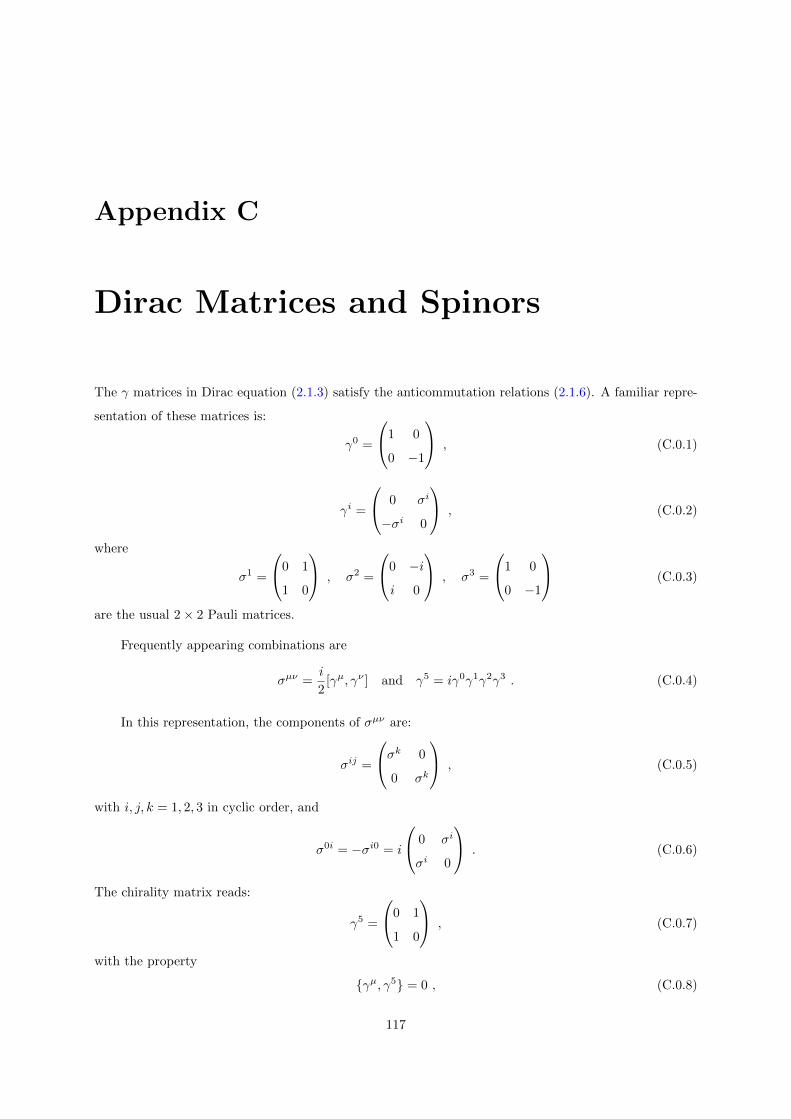
Appendix C
Dirac Matrices and Spinors
The γ matrices in Dirac equation (2.1.3) satisfy the anticommutation relations (2.1.6). A familiar repre-
sentation of these matrices is:
γ0 =
1 0
0 −1
, (C.0.1)
γi =
0 σi
−σi 0
, (C.0.2)
where
σ1 =
0 1
1 0
, σ2 =
0 −i
i 0
, σ3 =
1 0
0 −1
(C.0.3)
are the usual 2× 2 Pauli matrices.
Frequently appearing combinations are
σµν =i
2[γµ, γν ] and γ5 = iγ0γ1γ2γ3 . (C.0.4)
In this representation, the components of σµν are:
σij =
σk 0
0 σk
, (C.0.5)
with i, j, k = 1, 2, 3 in cyclic order, and
σ0i = −σi0 = i
0 σi
σi 0
. (C.0.6)
The chirality matrix reads:
γ5 =
0 1
1 0
, (C.0.7)
with the property
γµ, γ5 = 0 , (C.0.8)
117

Appendix C. Dirac Matrices and Spinors 118
which — in turn — implies that
[γ5, σµν ] = 0 . (C.0.9)
For the inner product of a γ matrix with an ordinary four-vector, we use the following notation:
γµAµ ≡ /A = γ0A0 − γ ·A, (C.0.10)
consistent with the metric signature (+,−,−,−).