cpt guide nov 2007 edition 2
TRANSCRIPT
8/13/2019 Cpt Guide Nov 2007 Edition 2
http://slidepdf.com/reader/full/cpt-guide-nov-2007-edition-2 1/126
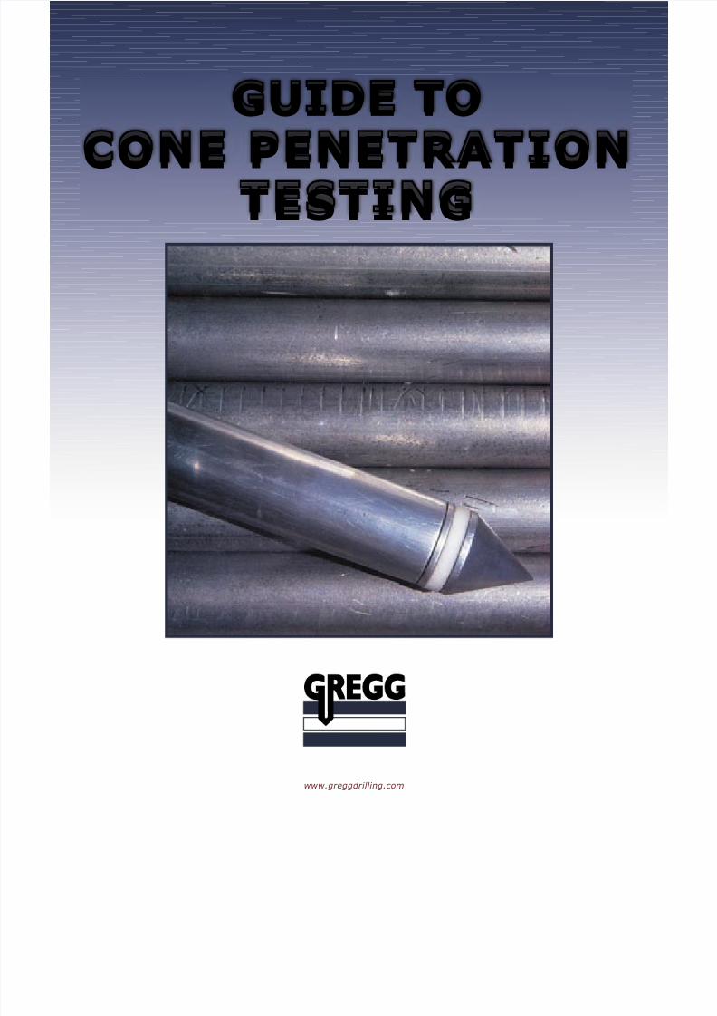
GUIDE TO
CONE PENETRATIONTESTING
www.greggdrilling.com

8/13/2019 Cpt Guide Nov 2007 Edition 2
http://slidepdf.com/reader/full/cpt-guide-nov-2007-edition-2 2/126
Engineering Units
Multiples
Micro () = 10-6
Milli (m) = 10-3
Kilo (k) = 10+3
Mega (M) = 10+6
Imperial Units SI Units
Length feet (ft) meter (m)
Area square feet (ft2) square meter (m
2)
Force pounds (p) Newton (N)
Pressure/Stress pounds/foot2(psf) Pascal (Pa) = (N/m
2)
Multiple UnitsLength inches (in) millimeter (mm)
Area square feet (ft2) square millimeter (mm2)
Force ton (t) kilonewton (kN)
Pressure/Stress pounds/inch2(psi) kilonewton/meter
2 kPa)
tons/foot2 (tsf) meganewton/meter
2(MPa)
Conversion Factors
Force: 1 ton = 9.8 kN1 kg = 9.8 N
Pressure/Stress 1kg/cm2 = 100 kPa = 100 kN/m
2 = 1 bar
1 tsf = 96 kPa (~100 kPa = 0.1 MPa)
1 t/m2 ~ 10 kPa
14.5 psi = 100 kPa
2.31 foot of water = 1 psi 1 meter of water = 10 kPa
Derived Values from CPT
Friction ratio: R f = (f s/qt) x 100%
Corrected cone resistance: qt = qc + u2(1-a)
Net cone resistance: qn = qt – vo
Excess pore pressure: �u = u2 – u0
Pore pressure ratio: Bq = �u / qn
Normalized excess pore pressure: U = (ut – u0) / (ui – u0)
where: ut is the pore pressure at timet
in a dissipation test, andui is the initial pore pressure at the start of the dissipation test
8/13/2019 Cpt Guide Nov 2007 Edition 2
http://slidepdf.com/reader/full/cpt-guide-nov-2007-edition-2 3/126
Guide to
Cone Penetration Testingfor
Geotechnical Engineering
By
P. K. Robertson
and
K.L. Cabal (Robertson)
Gregg Drilling & Testing, Inc.
2nd
Edition November 2007
8/13/2019 Cpt Guide Nov 2007 Edition 2
http://slidepdf.com/reader/full/cpt-guide-nov-2007-edition-2 4/126
Gregg Drilling & Testing, Inc.
Corporate Headquarters
2726 Walnut Avenue
Signal Hill, California 90755
Telephone: (562) 427-6899
Fax: (562) 427-3314
E-mail: [email protected]: www.greggdrilling.com
The publisher and the author make no warranties or representations of any kind concerning the accuracy orsuitability of the information contained in this guide for any purpose and cannot accept any legal
responsibility for any errors or omissions that may have been made.
Copyright © 2007 Gregg Drilling & Testing, Inc. All rights reserved.

8/13/2019 Cpt Guide Nov 2007 Edition 2
http://slidepdf.com/reader/full/cpt-guide-nov-2007-edition-2 5/126
TABLE OF CONTENTS
Glossary i
Introduction 1
Risk Based Site Characterization 2
Role of the CPT 3
Cone Penetration Test (CPT) 5
Introduction 5
History 6
Test Equipment and Procedures 9
Additional Sensors/Modules 10 Pushing Equipment 11
Depth of Penetration 15
Test Procedures 15
CPT Interpretation 18 Soil Profiling and Classification 19 Equivalent SPT N60 Profiles 25 Undrained Shear Strength (su) 28 Soil Sensitivity 29 Undrained Shear Strength Ratio (su/σ'vo) 30 Stress History - Overconsolidation Ratio (OCR) 31
In-Situ Stress Ratio (K o) 32 Friction Angle 33 Relative density (Dr ) 35 Stiffness and Modulus 37 Modulus from Shear Wave Velocity 38 Estimating Shear Wave Velocity from CPT 39 Identification of Unusual Soils Using the SCPT 40 Hydraulic Conductivity (k) 41 Consolidation Characteristics 44 Constrained Modulus 47
Applications of CPT Results 48 Shallow Foundation Design 49 Deep Foundation Design 72
Liquefaction 84 Ground Improvement Compaction Control 106 Design of Wick or Sand Drains 110
Main References 112

8/13/2019 Cpt Guide Nov 2007 Edition 2
http://slidepdf.com/reader/full/cpt-guide-nov-2007-edition-2 6/126
CPT Guide – 2007 Glossary
i
Glossary
This glossary contains the most commonly used terms related to CPT and are
presented in alphabetical order.
CPT
Cone penetration test.
CPTU
Cone penetration test with pore pressure measurement – piezocone
test.
Cone
The part of the cone penetrometer on which the cone resistance is
measured.Cone penetrometer
The assembly containing the cone, friction sleeve, and any other
sensors and measuring systems, as well as the connections to the push
rods.
Cone resistance, q c
The force acting on the cone, Qc, divided by the projected area of the
cone, Ac.
q c = Qc / Ac
Corrected cone resistance, q t
The cone resistance q c corrected for pore water effects.q t = q c + u2(1- an)
Data acquisition system
The system used to record the measurements made by the cone
penetrometer.
Dissipation test
A test when the decay of the pore pressure is monitored during a pause
in penetration.
Filter element
The porous element inserted into the cone penetrometer to allowtransmission of pore water pressure to the pore pressure sensor, while
maintaining the correct dimensions of the cone penetrometer.
Friction ratio, R f
The ratio, expressed as a percentage, of the sleeve friction, f s, to the
cone resistance, q t, both measured at the same depth.
R f = (f s/q t) x 100%

8/13/2019 Cpt Guide Nov 2007 Edition 2
http://slidepdf.com/reader/full/cpt-guide-nov-2007-edition-2 7/126
CPT Guide - 2007 Glossary
ii
Friction reducer
A local enlargement on the push rods placed a short distance above the
cone penetrometer, to reduce the friction on the push rods.
Friction sleeve
The section of the cone penetrometer upon which the sleeve friction is
measured.
Normalized cone resistance, Qt
The cone resistance expressed in a non-dimensional form and taking
account of the in-situ vertical stresses.
Qt = (q t – σvo) / σ'vo
Normalized cone resistance, Qtn
The cone resistance expressed in a non-dimensional form taking
account of the in-situ vertical stresses and where the stress exponent(n) varies with soil type. When n = 1, Qtn = Qt.
Qtn =
n
vo
a
a
vo P
P ⎟⎟ ⎠
⎞⎜⎜⎝
⎛ ⎟⎟ ⎠
⎞⎜⎜⎝
⎛ −'
qt
2 σ
σ
Net cone resistance, q n
The corrected cone resistance minus the vertical total stress.
q n = q t – σvo
Excess pore pressure (or net pore pressure), Δu
The measured pore pressure less the in-situ equilibrium pore pressure.
Δu = u2 – u0
Pore pressure
The pore pressure generated during cone penetration and measured by
a pore pressure sensor:
u1 when measured on the cone
u2 when measured just behind the cone.
Pore pressure ratio, Bq
The net pore pressure normalized with respect to the net cone
resistance.
Bq = Δu / q n Push rods
Thick-walled tubes used to advance the cone penetrometer
Sleeve friction, f s
The frictional force acting on the friction sleeve, Fs, divided by its
surface area, As.
f s = Fs / As
8/13/2019 Cpt Guide Nov 2007 Edition 2
http://slidepdf.com/reader/full/cpt-guide-nov-2007-edition-2 8/126
CPT Guide – 2007 Introduction
1
Introduction
The purpose of this guide is to provide a concise resource for the applicationof the CPT to geotechnical engineering practice. This guide is a supplement
and update to the book ‘CPT in Geotechnical Practice’ by Lunne, Robertson
and Powell (1997). This guide is applicable primarily to data obtained using
a standard electronic cone with a 60-degree apex angle and either a diameter
of 35.7 mm or 43.7 mm (10 or 15 cm2 cross-sectional area).
Recommendations are provided on applications of CPT data for soil
profiling, material identification and evaluation of geotechnical parameters
and design. The companion book provides more details on the history of the
CPT, equipment, specification and performance, as well as details ongeo-environmental applications. The book also provides extensive
background on interpretation techniques. This guide provides only the basic
recommendations for the application of the CPT for geotechnical design
A list of the main references is included at the end of this guide. A more
comprehensive reference list can be found in the companion CPT book.
8/13/2019 Cpt Guide Nov 2007 Edition 2
http://slidepdf.com/reader/full/cpt-guide-nov-2007-edition-2 9/126
CPT Guide - 2007 Risk Based Site Characterization
2
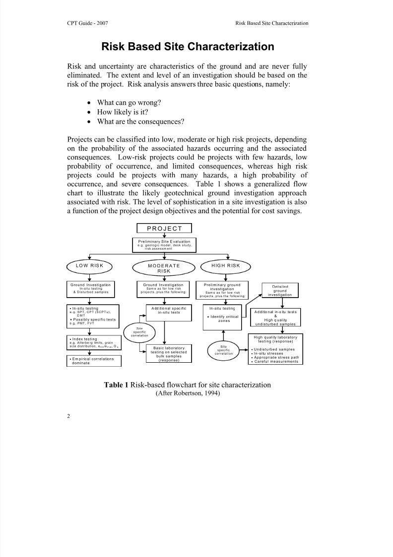
Risk Based Site Characterization
Risk and uncertainty are characteristics of the ground and are never fully
eliminated. The extent and level of an investigation should be based on the
risk of the project. Risk analysis answers three basic questions, namely:
• What can go wrong?
• How likely is it?
• What are the consequences?
Projects can be classified into low, moderate or high risk projects, depending
on the probability of the associated hazards occurring and the associated
consequences. Low-risk projects could be projects with few hazards, low
probability of occurrence, and limited consequences, whereas high risk projects could be projects with many hazards, a high probability of
occurrence, and severe consequences. Table 1 shows a generalized flow
chart to illustrate the likely geotechnical ground investigation approach
associated with risk. The level of sophistication in a site investigation is also
a function of the project design objectives and the potential for cost savings.
LO W R IS K H IG H R IS KM O D E R A T ERISK
P R O J E C T
Ground Invest igat ionIn-si tu test ing
& D is turbed samples
Ground Invest igat ionSam e as for l ow r i sk
pro jec ts , p lus the fo l low ing:
• In-si tu testinge . g . S P T , C P T (S C P T u) , D M T
• Possib ly speci f ic testse.g. PMT, FVT
A dd it io nal spec if icin-si tu tests
Sitespeci f ic
correlat ion
Pre l iminary groundinvestigation
Sam e as for l ow r i skpro jec ts , p lus the fo l low ing:
Deta i ledground
investigation
In-si tu testing
• Identi fy cri t ical zones
A ddi tio nal in -s itu te st s&
High q ua l i tyund is turbed samples
High qua l i ty laboratorytest ing ( response)
• Undisturbed samples• In -s i tu s tresses• Appropr ia te s tress path• Carefu l measurements
Pre l iminary Si te E va luat ione.g. geo log ic model , desk s tudy ,
r i sk assessm ent
Basic laboratorytest ing on se lected
bulk samples(response)
• Index test inge.g. Atterbe rg l imi ts, grainsize distr ibut ion, e m in /e m ax , G s Site
speci f iccor re la t ion
• Em pir ica l corre la t ions
dominate
Table 1 Risk-based flowchart for site characterization(After Robertson, 1994)

8/13/2019 Cpt Guide Nov 2007 Edition 2
http://slidepdf.com/reader/full/cpt-guide-nov-2007-edition-2 10/126
CPT Guide 2007 Role of the CPT
3
Role of the CPT
The objectives of any subsurface investigation are to determine the
following:
• Nature and sequence of the subsurface strata (geologic regime)
• Groundwater conditions (hydrologic regime)
• Physical and mechanical properties of the subsurface strata
For geo-environmental site investigations where contaminants are possible,
the above objectives have the additional requirement to determine:
• Distribution and composition of contaminants
The above requirements are a function of the proposed project and the
associated risks. An ideal investigation program should include a mix of
field and laboratory tests depending on the risk of the project.
Table 2 presents a partial list of the major in-situ tests and their perceived
applicability for use in different ground conditions.
Table 2 The applicability and usefulness of in-situ tests(Lunne, Robertson & Powell, 1997)
8/13/2019 Cpt Guide Nov 2007 Edition 2
http://slidepdf.com/reader/full/cpt-guide-nov-2007-edition-2 11/126
CPT Guide – 2007 Role of the CPT
4
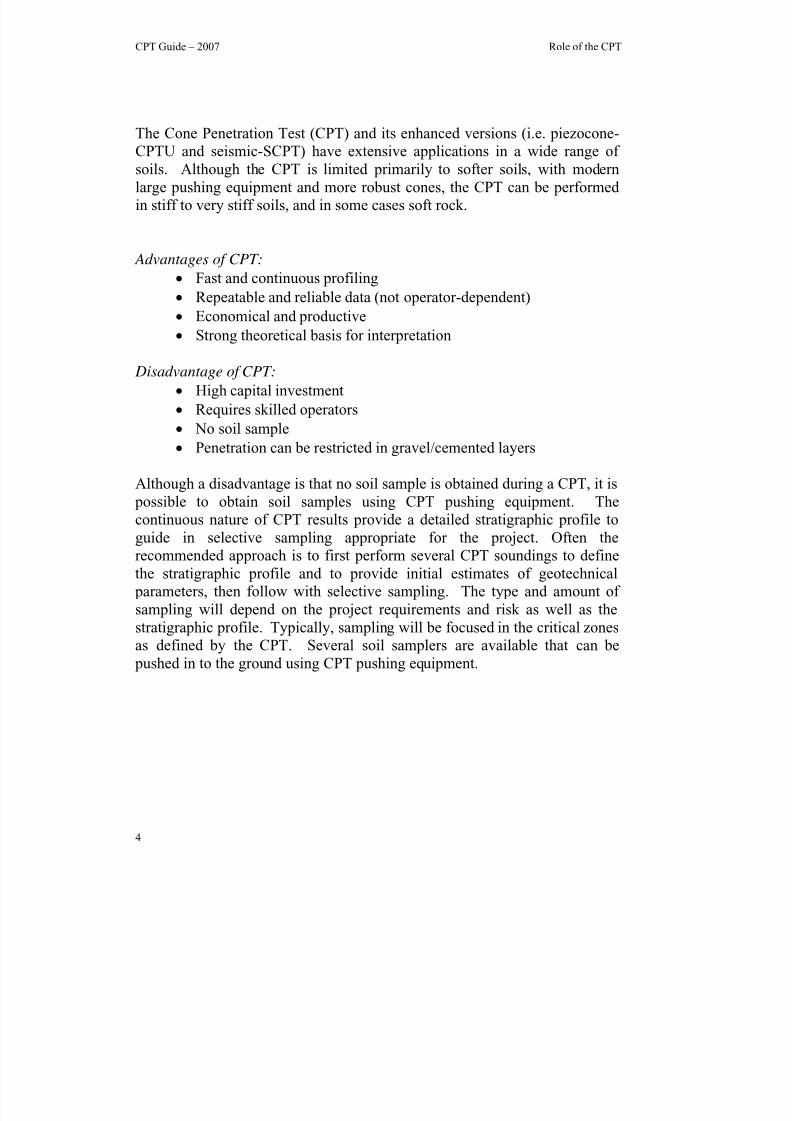
The Cone Penetration Test (CPT) and its enhanced versions (i.e. piezocone-
CPTU and seismic-SCPT) have extensive applications in a wide range of
soils. Although the CPT is limited primarily to softer soils, with modernlarge pushing equipment and more robust cones, the CPT can be performed
in stiff to very stiff soils, and in some cases soft rock.
Advantages of CPT:
• Fast and continuous profiling
• Repeatable and reliable data (not operator-dependent)
• Economical and productive
• Strong theoretical basis for interpretation
Disadvantage of CPT:
• High capital investment
• Requires skilled operators
• No soil sample
• Penetration can be restricted in gravel/cemented layers
Although a disadvantage is that no soil sample is obtained during a CPT, it is
possible to obtain soil samples using CPT pushing equipment. The
continuous nature of CPT results provide a detailed stratigraphic profile to
guide in selective sampling appropriate for the project. Often the
recommended approach is to first perform several CPT soundings to define
the stratigraphic profile and to provide initial estimates of geotechnical
parameters, then follow with selective sampling. The type and amount of
sampling will depend on the project requirements and risk as well as the
stratigraphic profile. Typically, sampling will be focused in the critical zones
as defined by the CPT. Several soil samplers are available that can be
pushed in to the ground using CPT pushing equipment.
8/13/2019 Cpt Guide Nov 2007 Edition 2
http://slidepdf.com/reader/full/cpt-guide-nov-2007-edition-2 12/126
CPT Guide - 2007 Cone Penetration Test (CPT)
5
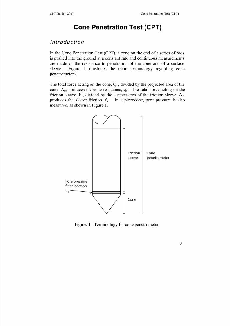
Cone Penetration Test (CPT)
In t roduct ion
In the Cone Penetration Test (CPT), a cone on the end of a series of rods
is pushed into the ground at a constant rate and continuous measurements
are made of the resistance to penetration of the cone and of a surface
sleeve. Figure 1 illustrates the main terminology regarding cone
penetrometers.
The total force acting on the cone, Qc, divided by the projected area of the
cone, Ac, produces the cone resistance, q c. The total force acting on the
friction sleeve, Fs, divided by the surface area of the friction sleeve, As,
produces the sleeve friction, f s. In a piezocone, pore pressure is alsomeasured, as shown in Figure 1.
Figure 1 Terminology for cone penetrometers

8/13/2019 Cpt Guide Nov 2007 Edition 2
http://slidepdf.com/reader/full/cpt-guide-nov-2007-edition-2 13/126
CPT Guide - 2007 Cone Penetration Test (CPT)
6
History
1932The first cone penetrometer tests were made using a 35 mm outside
diameter gas pipe with a 15 mm steel inner push rod. A cone tip with a 10cm
2 projected area and a 60
o apex angle was attached to the steel inner
push rods, as shown in Figure 2.
Figure 2 Early Dutch mechanical cone (After Sanglerat, 1972)
1935
Delf Soil Mechanics Laboratory designed the first manually operated 10ton (100 kN) cone penetration push machine, see Figure 3.
Figure 3 Early Dutch mechanical cone (After Delft Geotechnics)

8/13/2019 Cpt Guide Nov 2007 Edition 2
http://slidepdf.com/reader/full/cpt-guide-nov-2007-edition-2 14/126
CPT Guide - 2007 Cone Penetration Test (CPT)
7
1948The original Dutch mechanical cone was improved by adding a conical
part just above the cone. The purpose of the geometry was to prevent soil
from entering the gap between the casing and inner rods. The basic Dutch
mechanical cones, shown in Figure 4, are still in use in some parts of theworld.
Figure 4 Dutch mechanical cone penetrometer with conical mantle
1953A friction sleeve (‘adhesion jacket’) was added behind the cone to include
measurement of the local sleeve friction (Begemann, 1953), see Figure 5.
Measurements were made every 8 inches (20 cm), and for the first time,
friction ratio was used to classify soil type (see Figure 6).
Figure 5 Begemann type cone with friction sleeve

8/13/2019 Cpt Guide Nov 2007 Edition 2
http://slidepdf.com/reader/full/cpt-guide-nov-2007-edition-2 15/126
CPT Guide - 2007 Cone Penetration Test (CPT)
8
Figure 6 First soil classification for Begemann mechanical cone
1965Fugro developed an electric cone, of which the shape and dimensions
formed the basis for the modern cones and the International Reference
Test and ASTM procedure. The main improvements relative to the
mechanical cone penetrometers were:
• Elimination of incorrect readings due to friction between inner rods
and outer rods and weight of inner rods.• Continuous testing with continuous rate of penetration without the
need for alternate movements of different parts of the penetrometer
and no undesirable soil movements influencing the cone resistance.
• Simpler and more reliable electrical measurement of cone
resistance and sleeve friction.
1974
Cone penetrometers that could also measure pore pressure (piezocone)were introduced. Early design had various shapes and pore pressure filter
locations. Gradually the practice has become more standardized so that
the recommended position of the filter element is close behind the cone at
the u2 location. With the measurement of pore water pressure it became
apparent that it was necessary to correct the cone resistance for pore water
pressure effects (q t), especially in soft clay.

8/13/2019 Cpt Guide Nov 2007 Edition 2
http://slidepdf.com/reader/full/cpt-guide-nov-2007-edition-2 16/126
CPT Guide - 2007 Cone Penetration Test (CPT)
9
Test Equipm ent and Procedures
Cone Penetrometers
Cone penetrometers come in a range of sizes with the 10 cm2 and 15 cm
2
probes the most common and specified in most standards. Figure 7 shows
a range of cones from a mini-cone at 2 cm2 to a large cone at 40 cm
2. The
mini cones are used for shallow investigations, whereas the large cones
can be used in gravely soils.
Figure 7 Range of CPT probes (from left: 2 cm2, 10 cm
2, 15 cm
2, 40 cm
2)
8/13/2019 Cpt Guide Nov 2007 Edition 2
http://slidepdf.com/reader/full/cpt-guide-nov-2007-edition-2 17/126
CPT Guide - 2007 Cone Penetration Test (CPT)
10
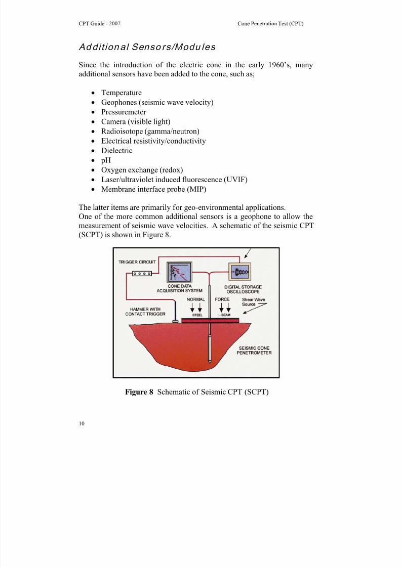
Addit ional Senso rs/Modu les
Since the introduction of the electric cone in the early 1960’s, many
additional sensors have been added to the cone, such as;
• Temperature
• Geophones (seismic wave velocity)
• Pressuremeter
• Camera (visible light)
• Radioisotope (gamma/neutron)
• Electrical resistivity/conductivity
• Dielectric
• pH
• Oxygen exchange (redox)• Laser/ultraviolet induced fluorescence (UVIF)
• Membrane interface probe (MIP)
The latter items are primarily for geo-environmental applications.
One of the more common additional sensors is a geophone to allow the
measurement of seismic wave velocities. A schematic of the seismic CPT
(SCPT) is shown in Figure 8.
Figure 8 Schematic of Seismic CPT (SCPT)
8/13/2019 Cpt Guide Nov 2007 Edition 2
http://slidepdf.com/reader/full/cpt-guide-nov-2007-edition-2 18/126
CPT Guide - 2007 Cone Penetration Test (CPT)
11
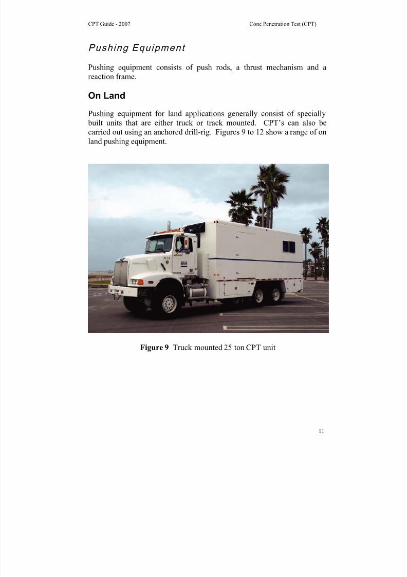
Pushing Equipment
Pushing equipment consists of push rods, a thrust mechanism and a
reaction frame.
On Land
Pushing equipment for land applications generally consist of specially
built units that are either truck or track mounted. CPT’s can also be
carried out using an anchored drill-rig. Figures 9 to 12 show a range of on
land pushing equipment.
Figure 9 Truck mounted 25 ton CPT unit

8/13/2019 Cpt Guide Nov 2007 Edition 2
http://slidepdf.com/reader/full/cpt-guide-nov-2007-edition-2 19/126
CPT Guide - 2007 Cone Penetration Test (CPT)
12
Figure 10 Track mounted 20 ton CPT unit
Figure 11 Small anchored drill-rig unit

8/13/2019 Cpt Guide Nov 2007 Edition 2
http://slidepdf.com/reader/full/cpt-guide-nov-2007-edition-2 20/126
CPT Guide - 2007 Cone Penetration Test (CPT)
13
Figure 12 Portable ramset for CPT inside buildings or limited access

8/13/2019 Cpt Guide Nov 2007 Edition 2
http://slidepdf.com/reader/full/cpt-guide-nov-2007-edition-2 21/126
CPT Guide - 2007 Cone Penetration Test (CPT)
14
Over Water
There is a variety of pushing equipment for over water investigations
depending on the depth of water. Floating or Jack-up barges are common
in shallow water (depth less than 30m/100 feet), see Figures 13 and 14.
Figure 13 Mid-size jack-up boat
Figure 14 Quinn Delta ship with spuds
8/13/2019 Cpt Guide Nov 2007 Edition 2
http://slidepdf.com/reader/full/cpt-guide-nov-2007-edition-2 22/126
CPT Guide - 2007 Cone Penetration Test (CPT)
15
Depth of Penetrat ion
CPT’s can be performed to depths exceeding 300 feet (100m) in soft soils
and with large capacity pushing equipment. To improve the depth of
penetration, the friction along the push rods should be reduced. This isnormally done by placing an expanded coupling (friction reducer) a short
distance (typically 3 feet, ~1m) behind the cone. Penetration will be
limited if either very hard soils, gravel layers or rock are encountered. It
is common to use 15 cm2 cones to increase penetration depth, since 15
cm2 cones are more robust and have a slightly larger diameter than the 10
cm2 push rods.
Test ProceduresPre-dri l l ing
For penetration in fills or hard soils it may be necessary to pre-drill in
order to avoid damaging the cone. Pre-drilling, in certain cases, may be
replaced by first pre-punching a hole through the upper problem material
with a solid steel dummy probe with a diameter slightly larger than the
cone. It is also common to hand auger the first 1.5m (5ft) in urban areas to
avoid underground utilities.
Vert ical i ty
The thrust machine should be set up so as to obtain a thrust direction as
near as possible to vertical. The deviation of the initial thrust direction
from vertical should not exceed 2 degrees and push rods should be
checked for straightness. Modern cones have simple slope sensors
incorporated to enable a measure of the non-verticality of the sounding.
This is useful to avoid damage to equipment and breaking of push rods.
For depths less than 50 feet (15m), significant non-verticality is unusual,
provided the initial thrust direction is vertical.
Reference Measurements
Modern cones have the potential for a high degree of accuracy and
repeatability (0.1% of full-scale output). Tests have shown that the zero
load output of the sensors can be sensitive to changes in temperature. It is

8/13/2019 Cpt Guide Nov 2007 Edition 2
http://slidepdf.com/reader/full/cpt-guide-nov-2007-edition-2 23/126
CPT Guide - 2007 Cone Penetration Test (CPT)
16
common practice to record zero load readings of all sensors to track these
changes.
Rate of Penetrat ion
The standard rate of penetration is 2 cm/sec (approximately 1 inch per
second). Hence, a 60 foot (20m) sounding can be completed (start to
finish) in about 30 minutes. The cone results are generally not sensitive to
slight variations in the rate of penetration.
Interval of readings
Electric cones produce continuous analogue data. However, most systems
convert the data to digital form at selected intervals. Most standards
require the interval to be no more than 8 inches (200mm). In general,most systems collect data at intervals of between 1 to 2 inches (25 -
50mm), with 2 inches (50 mm) being the most common.
Dissipat ion Tests
During a pause in penetration, any excess pore pressure generated around
the cone will start to dissipate. The rate of dissipation depends upon the
coefficient of consolidation, which in turn, depends on the compressibility
and permeability of the soil. The rate of dissipation also depends on the
diameter of the probe. A dissipation test can be performed at any requireddepth by stopping the penetration and measuring the decay of pore
pressure with time. If equilibrium pore pressures are required, the
dissipation test should continue until no further dissipation is observed.
This can occur rapidly in sands, but may take many hours in plastic clays.
Dissipation rate increases as probe size decreases.
Calibrat ion and Maintenance
Calibrations should be carried out at regular intervals (approximatelyevery 3 months). For major projects, check calibrations should be carried
out before and after the field work, with functional checks during the
work. Functional checks should include recording and evaluating the zero
load measurements (baseline).
8/13/2019 Cpt Guide Nov 2007 Edition 2
http://slidepdf.com/reader/full/cpt-guide-nov-2007-edition-2 24/126
CPT Guide - 2007 Cone Penetration Test (CPT)
17
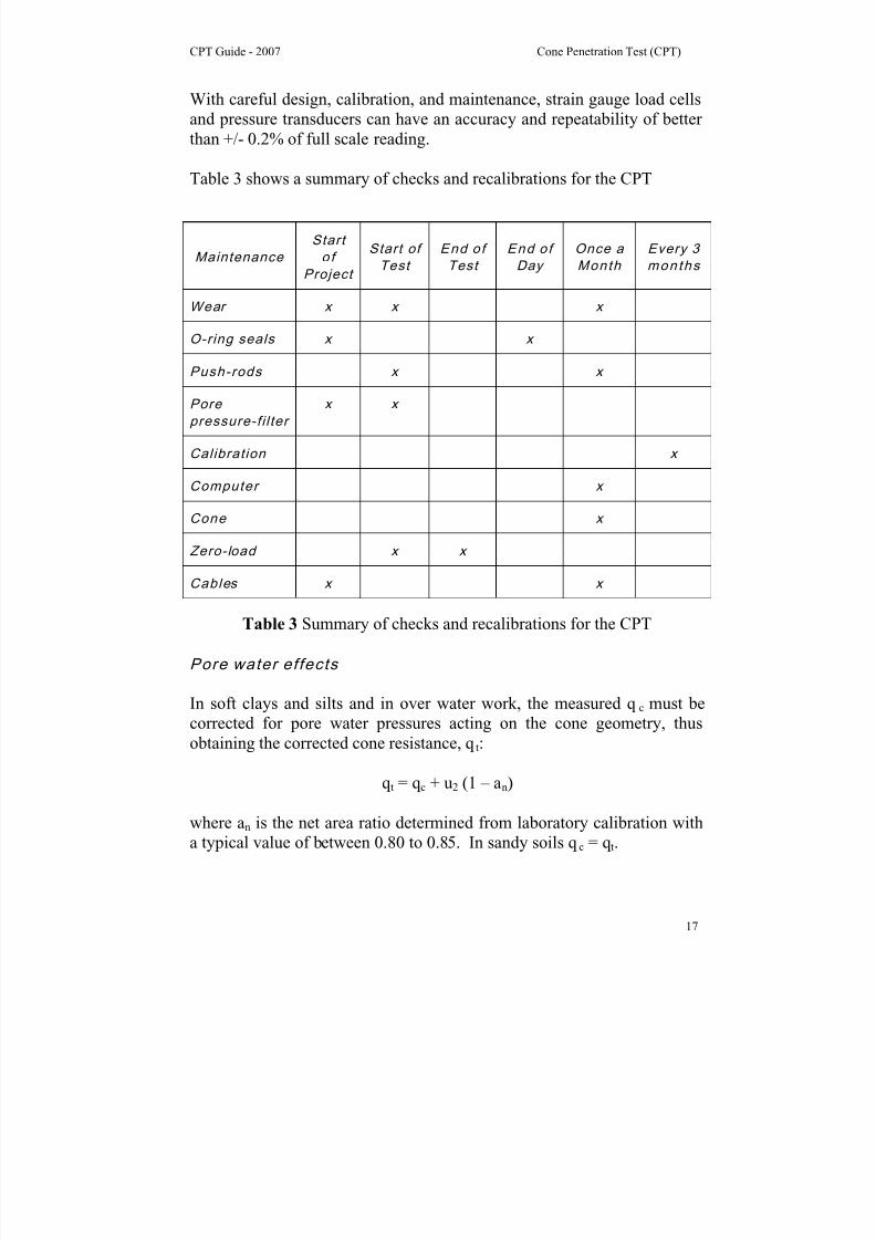
With careful design, calibration, and maintenance, strain gauge load cells
and pressure transducers can have an accuracy and repeatability of better
than +/- 0.2% of full scale reading.
Table 3 shows a summary of checks and recalibrations for the CPT
Maintenance
Start
o f
Project
Start of
Test
End of
Test
End of
Day
Once a
Month
Every 3
months
Wear x x x
O-ring seals x x
Push-rods x x
Pore
pressure-f i l ter
x x
Calibration x
Computer x
Cone x
Zero-load x x
Cables x x
Table 3 Summary of checks and recalibrations for the CPT
Pore water effects
In soft clays and silts and in over water work, the measured q c must be
corrected for pore water pressures acting on the cone geometry, thus
obtaining the corrected cone resistance, q t:
q t = q c + u2 (1 – an)
where an is the net area ratio determined from laboratory calibration with
a typical value of between 0.80 to 0.85. In sandy soils q c = q t.
8/13/2019 Cpt Guide Nov 2007 Edition 2
http://slidepdf.com/reader/full/cpt-guide-nov-2007-edition-2 25/126
CPT Guide - 2007 Cone Penetration Test (CPT)
18
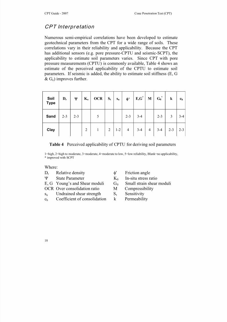
CPT Interpr etat ion
Numerous semi-empirical correlations have been developed to estimate
geotechnical parameters from the CPT for a wide range of soils. These
correlations vary in their reliability and applicability. Because the CPThas additional sensors (e.g. pore pressure-CPTU and seismic-SCPT), the
applicability to estimate soil parameters varies. Since CPT with pore
pressure measurements (CPTU) is commonly available, Table 4 shows an
estimate of the perceived applicability of the CPTU to estimate soil
parameters. If seismic is added, the ability to estimate soil stiffness (E, G
& Go) improves further.
SoilType
Dr Ψ K o OCR St su φ' E,G*
M G0* k ch
Sand 2-3 2-3 5 2-3 3-4 2-3 3 3-4
Clay 2 1 2 1-2
4 3-4 4 3-4 2-3 2-3
Table 4 Perceived applicability of CPTU for deriving soil parameters
1=high, 2=high to moderate, 3=moderate, 4=moderate to low, 5=low reliability, Blank=no applicability,
* improved with SCPT
Where:
Dr Relative density φ' Friction angle
Ψ State Parameter K 0 In-situ stress ratio
E, G Young’s and Shear moduli G0 Small strain shear moduli
OCR Over consolidation ratio M Compressibility
su Undrained shear strength St Sensitivitych Coefficient of consolidation k Permeability
8/13/2019 Cpt Guide Nov 2007 Edition 2
http://slidepdf.com/reader/full/cpt-guide-nov-2007-edition-2 26/126
CPT Guide - 2007 Cone Penetration Test (CPT)
19
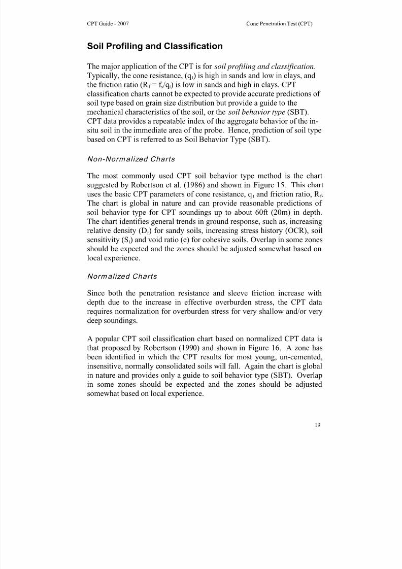
Soil Profiling and Classification
The major application of the CPT is for soil profiling and classification.
Typically, the cone resistance, (q t) is high in sands and low in clays, and
the friction ratio (R f = f s/q t) is low in sands and high in clays. CPTclassification charts cannot be expected to provide accurate predictions of
soil type based on grain size distribution but provide a guide to the
mechanical characteristics of the soil, or the soil behavior type (SBT).
CPT data provides a repeatable index of the aggregate behavior of the in-
situ soil in the immediate area of the probe. Hence, prediction of soil type
based on CPT is referred to as Soil Behavior Type (SBT).
Non-Normal ized Charts
The most commonly used CPT soil behavior type method is the chartsuggested by Robertson et al. (1986) and shown in Figure 15. This chart
uses the basic CPT parameters of cone resistance, q t and friction ratio, R f .
The chart is global in nature and can provide reasonable predictions of
soil behavior type for CPT soundings up to about 60ft (20m) in depth.
The chart identifies general trends in ground response, such as, increasing
relative density (Dr ) for sandy soils, increasing stress history (OCR), soil
sensitivity (St) and void ratio (e) for cohesive soils. Overlap in some zones
should be expected and the zones should be adjusted somewhat based on
local experience.
Normal ized Charts
Since both the penetration resistance and sleeve friction increase with
depth due to the increase in effective overburden stress, the CPT data
requires normalization for overburden stress for very shallow and/or very
deep soundings.
A popular CPT soil classification chart based on normalized CPT data is
that proposed by Robertson (1990) and shown in Figure 16. A zone has been identified in which the CPT results for most young, un-cemented,
insensitive, normally consolidated soils will fall. Again the chart is global
in nature and provides only a guide to soil behavior type (SBT). Overlap
in some zones should be expected and the zones should be adjusted
somewhat based on local experience.

8/13/2019 Cpt Guide Nov 2007 Edition 2
http://slidepdf.com/reader/full/cpt-guide-nov-2007-edition-2 27/126
CPT Guide - 2007 Cone Penetration Test (CPT)
20
Zone Soil Behavior Type
1
2
3
45
6
7
8
9
10
11
12
Sensitive fine grained
Organic material
Clay
Silty Clay to clayClayey silt to silty clay
Sandy silt to clayey silt
Silty sand to sandy silt
Sand to silty sand
Sand
Gravelly sand to sand
Very stiff fine grained*
Sand to clayey sand*
* Overconsolidated or cemented
1 MPa = 10 tsf
Figure 15 CPT Soil Behavior Type (SBT) chart(Robertson et al., 1986).

8/13/2019 Cpt Guide Nov 2007 Edition 2
http://slidepdf.com/reader/full/cpt-guide-nov-2007-edition-2 28/126
CPT Guide - 2007 Cone Penetration Test (CPT)
21
Zone Soil Behavior Type I c
1 Sensitive, fine grained N/A
2 Organic soils – peats > 3.6
3 Clays – silty clay to clay 2.95 – 3.6
4 Silt mixtures – clayey silt tosilty clay
2.60 – 2.95
5 Sand mixtures – silty sand to
sandy silt
2.05 – 2.6
6 Sands – clean sand to silty
sand
1.31 – 2.05
7 Gravelly sand to dense sand < 1.31
8 Very stiff sand to clayey sand* N/A
9 Very stiff, fine grained* N/A
* Heavily overconsolidated or cemented
Figure 16 Normalized CPT Soil Behavior Type (SBT N) chart, Qt - F(Robertson, 1990).

8/13/2019 Cpt Guide Nov 2007 Edition 2
http://slidepdf.com/reader/full/cpt-guide-nov-2007-edition-2 29/126
CPT Guide - 2007 Cone Penetration Test (CPT)
22
The full normalized SBT N charts suggested by Robertson (1990) also
included an additional chart based on normalized pore pressure parameter,
Bq , as shown on Figure 17, where;
Bq = Δu / q n
and; excess pore pressure, Δu = u2 – u0
net cone resistance, q n = q t – σvo
The Qt – Bq chart can aid in the identification of saturated fine grained
soils where the excess CPT penetration pore pressures can be large. In
general, the Qt - Bq chart is not commonly used due to the lack of
repeatability of the pore pressure results (e.g. poor saturation or loss of
saturation of the filter element, etc.)
Figure 17 Normalized CPT Soil Behavior Type (SBT N) charts
Qt – Fr and Qt - Bq (Robertson, 1990).

8/13/2019 Cpt Guide Nov 2007 Edition 2
http://slidepdf.com/reader/full/cpt-guide-nov-2007-edition-2 30/126
CPT Guide - 2007 Cone Penetration Test (CPT)
23
If no prior CPT experience exists in a given geologic environment it is
advisable to obtain samples from appropriate locations to verify the
classification and soil behavior type. If significant CPT experience is
available and the charts have been modified based on this experience
samples may not be required.
Soil classification can be improved if pore pressure data is also collected,
as shown on Figure 17. In soft clay the penetration pore pressures can be
very large, whereas, in stiff heavily over-consolidated clays or dense silts
and silty sands the penetration pore pressures can be small and sometimes
negative relative to the equilibrium pore pressures (u0). The rate of pore
pressure dissipation during a pause in penetration can guide in the soil
type. In sandy soils any excess pore pressures will dissipate very quickly,
whereas, in clays the rate of dissipation can be very slow.
To simplify the application of the CPT SBTN chart shown in Figure 16,
the normalized cone parameters Qt and Fr can be combined into one Soil
Behavior Type index, Ic, where Ic is the radius of the essentially
concentric circles that represent the boundaries between each SBT zone.
Ic can be defined as follows;
Ic = ((3.47 - log Qt)2 + (log Fr + 1.22)
2)
0.5
where:
Qt = normalized cone penetration resistance (dimensionless)
= (q t – σvo)/σ'vo
Fr = normalized friction ratio, in %
= (f s/(q t – σvo)) x 100%
The term Qt represents the simple stress normalization with a stress
exponent (n) of 1.0, which applies well to clay-like soils. Recently
Robertson suggested that the normalized SBT N charts shown in Figures
16 and 17 should be used with the normalized cone resistance calculated by using a stress exponent that varies with soil type via Ic (i.e. Qtn, see
Figure 37).
The boundaries of soil behavior types are then given in terms of the index,
Ic, as shown in Figure 16. The soil behavior type index does not apply to
zones 1, 8 and 9. Profiles of Ic provide a simple guide to the continuous
8/13/2019 Cpt Guide Nov 2007 Edition 2
http://slidepdf.com/reader/full/cpt-guide-nov-2007-edition-2 31/126
CPT Guide - 2007 Cone Penetration Test (CPT)
24
variation of soil behavior type in a given soil profile based on CPT results.
Independent studies have shown that the normalized SBT N chart shown in
Figure 16 typically has greater than 80% reliability when compared with
samples.
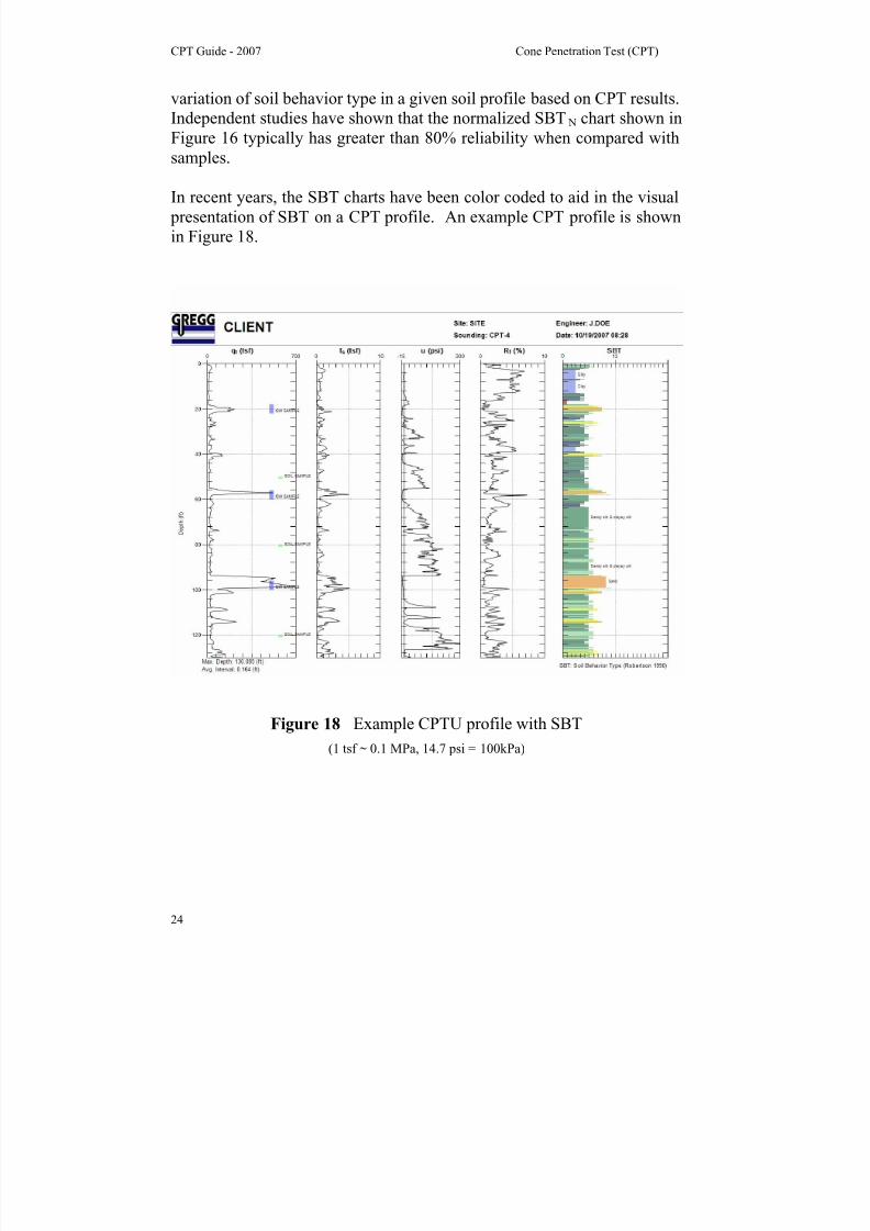
In recent years, the SBT charts have been color coded to aid in the visual
presentation of SBT on a CPT profile. An example CPT profile is shown
in Figure 18.
Figure 18 Example CPTU profile with SBT
(1 tsf ~ 0.1 MPa, 14.7 psi = 100kPa)
8/13/2019 Cpt Guide Nov 2007 Edition 2
http://slidepdf.com/reader/full/cpt-guide-nov-2007-edition-2 32/126
CPT Guide - 2007 Cone Penetration Test (CPT)
25
Equivalent SPT N60 Profiles
The Standard Penetration Test (SPT) is one of the most commonly used
in-situ tests in many parts of the world, especially North America.
Despite continued efforts to standardize the SPT procedure and equipmentthere are still problems associated with its repeatability and reliability.
However, many geotechnical engineers have developed considerable
experience with design methods based on local SPT correlations. When
these engineers are first introduced to the CPT they initially prefer to see
CPT results in the form of equivalent SPT N-values. Hence, there is a
need for reliable CPT/SPT correlations so that CPT data can be used in
existing SPT-based design approaches.
There are many factors affecting the SPT results, such as borehole
preparation and size, sampler details, rod length and energy efficiency ofthe hammer-anvil-operator system. One of the most significant factors is
the energy efficiency of the SPT system. This is normally expressed in
terms of the rod energy ratio (ERr). An energy ratio of about 60% has
generally been accepted as the reference value which represents the
approximate historical average SPT energy.
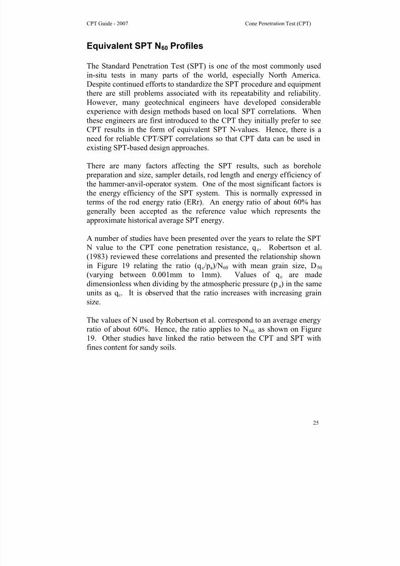
A number of studies have been presented over the years to relate the SPT
N value to the CPT cone penetration resistance, q c. Robertson et al.
(1983) reviewed these correlations and presented the relationship shownin Figure 19 relating the ratio (q c/pa)/N60 with mean grain size, D50
(varying between 0.001mm to 1mm). Values of q c are made
dimensionless when dividing by the atmospheric pressure (pa) in the same
units as q c. It is observed that the ratio increases with increasing grain
size.
The values of N used by Robertson et al. correspond to an average energy
ratio of about 60%. Hence, the ratio applies to N60, as shown on Figure
19. Other studies have linked the ratio between the CPT and SPT with
fines content for sandy soils.

8/13/2019 Cpt Guide Nov 2007 Edition 2
http://slidepdf.com/reader/full/cpt-guide-nov-2007-edition-2 33/126
CPT Guide - 2007 Cone Penetration Test (CPT)
26
Figure 19 CPT-SPT correlations with mean grain size(Robertson et al., 1983)
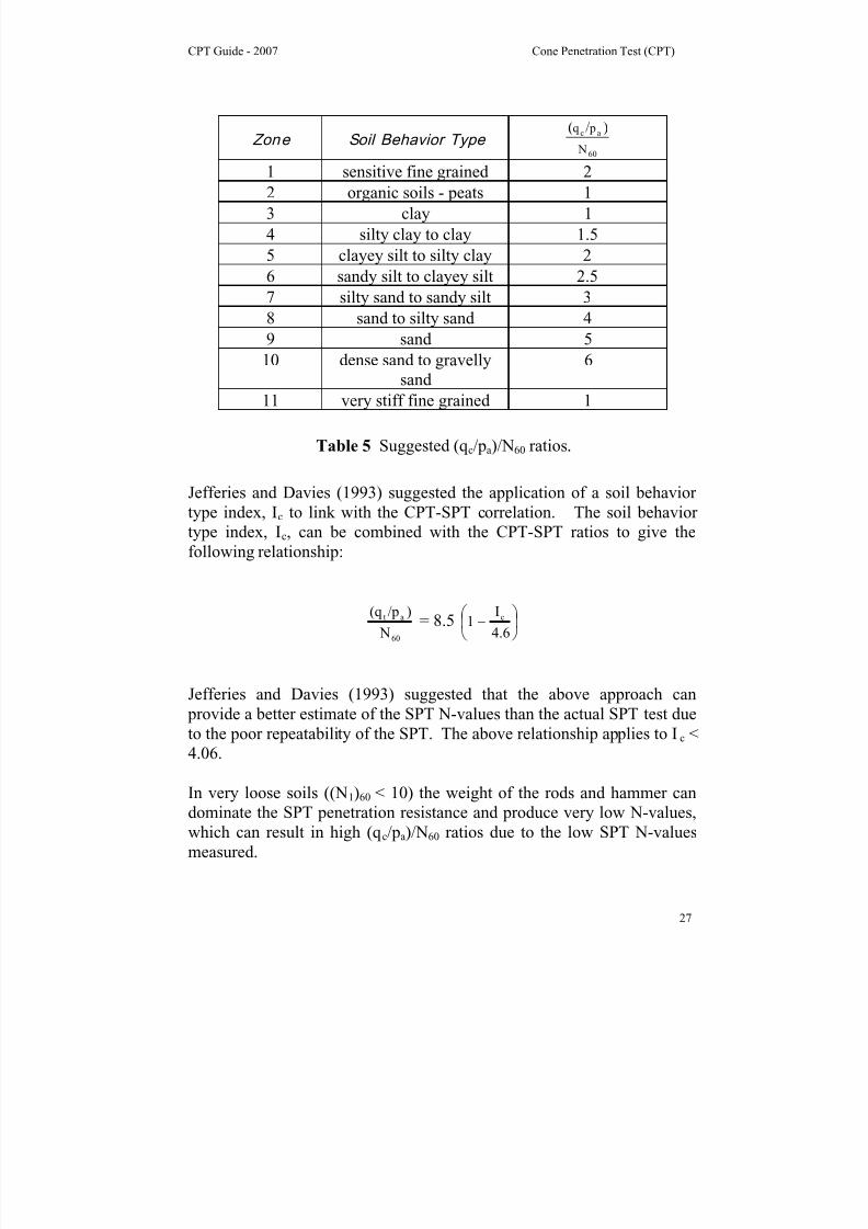
The above correlations require the soil grain size information to determine
the mean grain size (or fines content). Grain characteristics can be
estimated directly from CPT results using soil classification or soil
behavior type (SBT) charts. The CPT SBT charts show a clear trend of
increasing friction ratio with increasing fines content and decreasing grainsize. Robertson et al. (1986) suggested (q c/pa)/N60 ratios for each soil
behavior type zone using the non-normalized CPT chart. The suggested
ratio for each soil behavior type is given in Table 5.
These values provide a reasonable estimate of SPT N60 values from CPT
data. For simplicity the above correlations are given in terms of q c. For
fine grained soft soils the correlations should be applied to total cone
resistance, q t. Note that in sandy soils q c = q t.
One disadvantage of this simplified approach is the somewhatdiscontinuous nature of the conversion. Often a soil will have CPT data
that crosses different soil behavior type zones and hence produces
discontinuous changes in predicted SPT N60 values.
8/13/2019 Cpt Guide Nov 2007 Edition 2
http://slidepdf.com/reader/full/cpt-guide-nov-2007-edition-2 34/126
CPT Guide - 2007 Cone Penetration Test (CPT)
27
Zone Soil Behavior Type60
ac
N
pq )/(
1 sensitive fine grained 2
2 organic soils - peats 1
3 clay 1
4 silty clay to clay 1.5
5 clayey silt to silty clay 2
6 sandy silt to clayey silt 2.5
7 silty sand to sandy silt 3
8 sand to silty sand 4
9 sand 5
10 dense sand to gravelly
sand
6
11 very stiff fine grained 1
Table 5 Suggested (q c/pa)/N60 ratios.
Jefferies and Davies (1993) suggested the application of a soil behavior
type index, Ic to link with the CPT-SPT correlation. The soil behavior
type index, Ic, can be combined with the CPT-SPT ratios to give the
following relationship:
60
at
N
)/p(q = 8.5 ⎟
⎠
⎞⎜⎝
⎛ −
4.6
I1 c
Jefferies and Davies (1993) suggested that the above approach can
provide a better estimate of the SPT N-values than the actual SPT test due
to the poor repeatability of the SPT. The above relationship applies to Ic <
4.06.
In very loose soils ((N1)60 < 10) the weight of the rods and hammer can
dominate the SPT penetration resistance and produce very low N-values,
which can result in high (q c/pa)/N60 ratios due to the low SPT N-values
measured.
8/13/2019 Cpt Guide Nov 2007 Edition 2
http://slidepdf.com/reader/full/cpt-guide-nov-2007-edition-2 35/126
CPT Guide - 2007 Cone Penetration Test (CPT)
28
Undrained Shear Strength (su)
No single value of undrained shear strength exists, since the undrained
response of soil depends on the direction of loading, soil anisotropy, strainrate, and stress history. Typically the undrained strength in tri-axial
compression is larger than in simple shear which is larger than tri-axial
extension (suTC > suSS > suTE ). The value of su to be used in analysis
therefore depends on the design problem. In general, the simple shear
direction of loading often represents the average undrained strength.
Since anisotropy and strain rate will inevitably influence the results of all
in-situ tests, their interpretation will necessarily require some empirical
content to account for these factors, as well as possible effects of sample
disturbance.
Recent theoretical solutions have provided some valuable insight into the
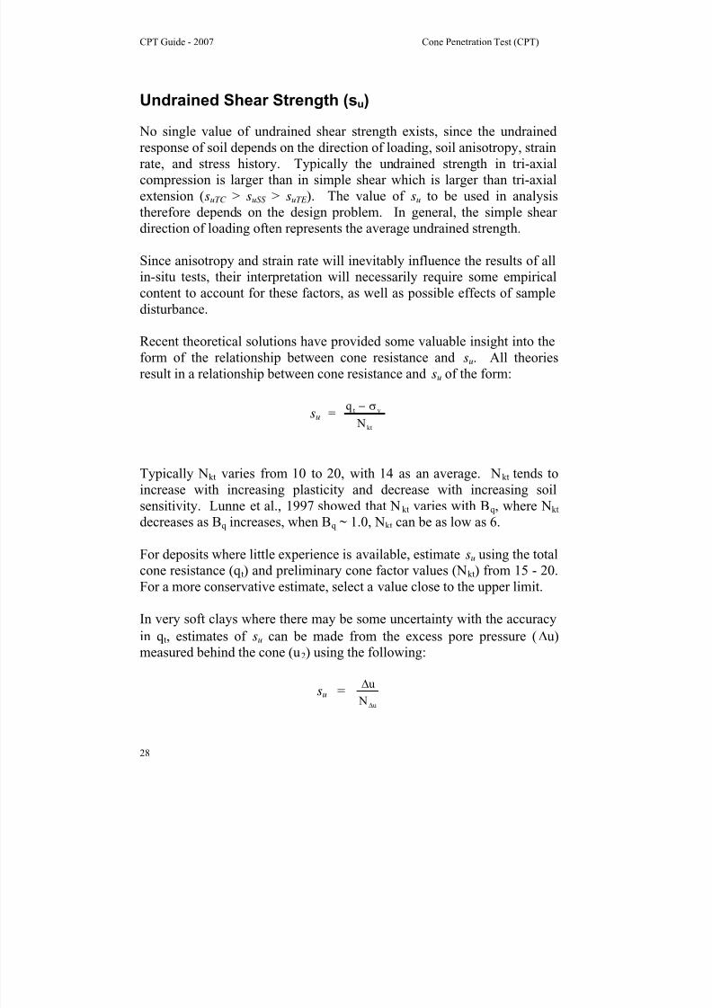
form of the relationship between cone resistance and su. All theories
result in a relationship between cone resistance and su of the form:
su =kt
vt
N
q σ−
Typically Nkt varies from 10 to 20, with 14 as an average. Nkt tends to
increase with increasing plasticity and decrease with increasing soil
sensitivity. Lunne et al., 1997 showed that Nkt varies with Bq , where Nkt
decreases as Bq increases, when Bq ~ 1.0, Nkt can be as low as 6.
For deposits where little experience is available, estimate su using the total
cone resistance (q t) and preliminary cone factor values (Nkt) from 15 - 20.
For a more conservative estimate, select a value close to the upper limit.
In very soft clays where there may be some uncertainty with the accuracy
in q t, estimates of su can be made from the excess pore pressure (Δu)
measured behind the cone (u2) using the following:
su =u N
u
Δ
Δ
8/13/2019 Cpt Guide Nov 2007 Edition 2
http://slidepdf.com/reader/full/cpt-guide-nov-2007-edition-2 36/126
CPT Guide - 2007 Cone Penetration Test (CPT)
29
Where NΔu varies from 4 to 8. For a more conservative estimate, select a
value close to the upper limit. Note that NΔu is linked to Nkt, via Bq ,
where:
NΔu = Bq Nkt
If previous experience is available in the same deposit, the values
suggested above should be adjusted to reflect this experience.
For larger, moderate to high risk projects, where high quality field and
laboratory data may be available, site specific correlations should be
developed based on appropriate and reliable values of su.
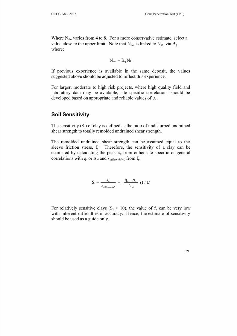
Soil Sensitivity
The sensitivity (St) of clay is defined as the ratio of undisturbed undrained
shear strength to totally remolded undrained shear strength.
The remolded undrained shear strength can be assumed equal to the
sleeve friction stress, f s. Therefore, the sensitivity of a clay can be
estimated by calculating the peak su from either site specific or generalcorrelations with q t or Δu and su(Remolded) from f s.
St =(Remolded)u
u
s
s =
kt
vt
N
q σ− (1 / f s)
For relatively sensitive clays (St > 10), the value of f s can be very low
with inherent difficulties in accuracy. Hence, the estimate of sensitivity
should be used as a guide only.

8/13/2019 Cpt Guide Nov 2007 Edition 2
http://slidepdf.com/reader/full/cpt-guide-nov-2007-edition-2 37/126
CPT Guide - 2007 Cone Penetration Test (CPT)
30
Undrained Shear Strength Ratio (su /σ'vo)
It is often useful to estimate the undrained shear strength ratio from the
CPT, since this relates directly to overconsolidation ratio (OCR). Critical
State Soil Mechanics presents a relationship between the undrained shear
strength ratio for normally consolidated clays under different directions of
loading and the effective stress friction angle, φ'. Hence, a better estimate
of undrained shear strength ratio can be obtained with knowledge of the
friction angle ((su /σ'vo) NC increases with increasing φ'). For normally
consolidated clays:
(su /σ'vo) NC = 0.22 in direct simple shear (φ' = 26o)
From the CPT:
(su /σ'vo) = ⎟⎟ ⎠
⎞⎜⎜⎝
⎛
σ
σ−
vo
vot
'
q (1/Nkt) = Qt / Nkt
Since Nkt ~ 14 (su /σ'vo) ~ 0.071 Qt
For a normally consolidated clay where (su /σ'vo) NC = 0.22;
Qt ~ 3
Based on the assumption that the sleeve friction measures the remolded
shear strength, suRemolded = f s
Therefore:
su /σ'vo = f s /σ'vo = (F . Qt) / 100
Hence, it is possible to represent (su /σ'vo) contours on the normalized
SBT N chart (Figure 16). These contours represent OCR for insensitive
clays with high values of (su /σ'vo) and Sensitivity for low values of
(su /σ'vo).
8/13/2019 Cpt Guide Nov 2007 Edition 2
http://slidepdf.com/reader/full/cpt-guide-nov-2007-edition-2 38/126
CPT Guide - 2007 Cone Penetration Test (CPT)
31
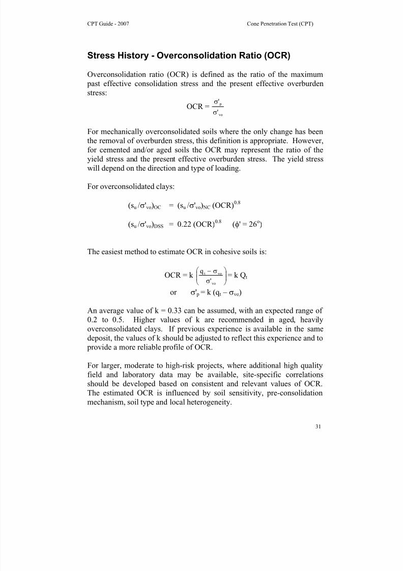
Stress History - Overconsolidation Ratio (OCR)
Overconsolidation ratio (OCR) is defined as the ratio of the maximum
past effective consolidation stress and the present effective overburdenstress:
OCR =vo
p
'
'
σ
σ
For mechanically overconsolidated soils where the only change has been
the removal of overburden stress, this definition is appropriate. However,
for cemented and/or aged soils the OCR may represent the ratio of the
yield stress and the present effective overburden stress. The yield stress
will depend on the direction and type of loading.
For overconsolidated clays:
(su /σ'vo)OC = (su /σ'vo) NC (OCR)0.8
(su /σ'vo)DSS = 0.22 (OCR)0.8
(φ' = 26o)
The easiest method to estimate OCR in cohesive soils is:
OCR = k ⎟⎟ ⎠
⎞⎜⎜⎝
⎛
σ
σ−
vo
vot
'
q = k Qt
or σ' p = k (q t – σvo)
An average value of k = 0.33 can be assumed, with an expected range of
0.2 to 0.5. Higher values of k are recommended in aged, heavily
overconsolidated clays. If previous experience is available in the same
deposit, the values of k should be adjusted to reflect this experience and to
provide a more reliable profile of OCR.
For larger, moderate to high-risk projects, where additional high quality
field and laboratory data may be available, site-specific correlations
should be developed based on consistent and relevant values of OCR.
The estimated OCR is influenced by soil sensitivity, pre-consolidation
mechanism, soil type and local heterogeneity.

8/13/2019 Cpt Guide Nov 2007 Edition 2
http://slidepdf.com/reader/full/cpt-guide-nov-2007-edition-2 39/126
CPT Guide - 2007 Cone Penetration Test (CPT)
32
In-Situ Stress Ratio (Ko)
There is no reliable method to determine K o from CPT. However, anestimate can be made based on an estimate of OCR, as shown in Figure
20.
Kulhawy and Mayne (1990) suggested a similar approach, using:
K o = 0.1 ⎟⎟ ⎠
⎞⎜⎜⎝
⎛
σ
σ−
vo
vot
'
q
These approaches are generally limited to mechanically overconsolidatedsoils. Considerable scatter exists in the database used for these
correlations and therefore they must be considered only as a guide.
Figure 20 OCR and K o from su/σ'vo and Plasticity Index, I p(after Andresen et al., 1979)
8/13/2019 Cpt Guide Nov 2007 Edition 2
http://slidepdf.com/reader/full/cpt-guide-nov-2007-edition-2 40/126
CPT Guide - 2007 Cone Penetration Test (CPT)
33
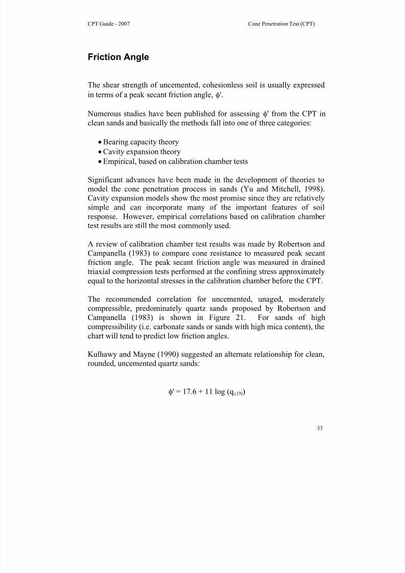
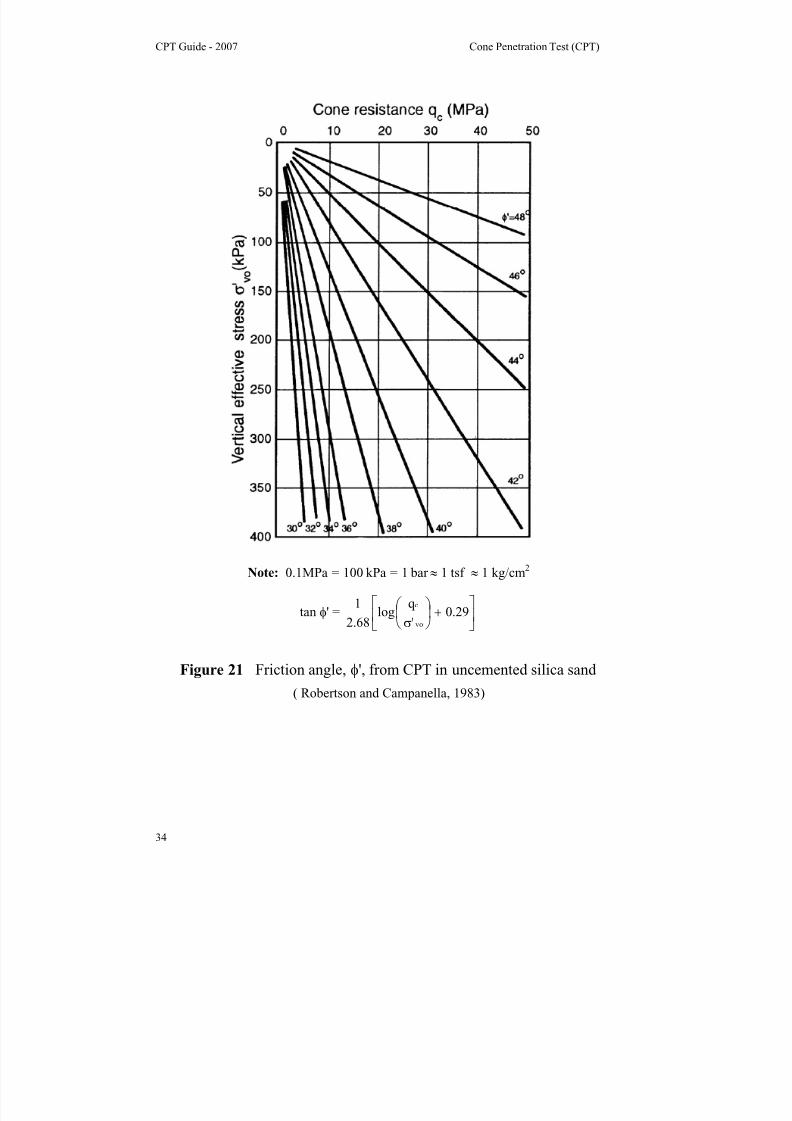
Friction Angle
The shear strength of uncemented, cohesionless soil is usually expressedin terms of a peak secant friction angle, φ'.
Numerous studies have been published for assessing φ' from the CPT in
clean sands and basically the methods fall into one of three categories:
• Bearing capacity theory
• Cavity expansion theory
• Empirical, based on calibration chamber tests
Significant advances have been made in the development of theories to
model the cone penetration process in sands (Yu and Mitchell, 1998).
Cavity expansion models show the most promise since they are relatively
simple and can incorporate many of the important features of soil
response. However, empirical correlations based on calibration chamber
test results are still the most commonly used.
A review of calibration chamber test results was made by Robertson and
Campanella (1983) to compare cone resistance to measured peak secant
friction angle. The peak secant friction angle was measured in drainedtriaxial compression tests performed at the confining stress approximately
equal to the horizontal stresses in the calibration chamber before the CPT.
The recommended correlation for uncemented, unaged, moderately
compressible, predominately quartz sands proposed by Robertson and
Campanella (1983) is shown in Figure 21. For sands of high
compressibility (i.e. carbonate sands or sands with high mica content), the
chart will tend to predict low friction angles.
Kulhawy and Mayne (1990) suggested an alternate relationship for clean,
rounded, uncemented quartz sands:
φ' = 17.6 + 11 log (q c1N)
8/13/2019 Cpt Guide Nov 2007 Edition 2
http://slidepdf.com/reader/full/cpt-guide-nov-2007-edition-2 41/126
CPT Guide - 2007 Cone Penetration Test (CPT)
34
Note: 0.1MPa = 100 kPa = 1 bar ≈ 1 tsf ≈ 1 kg/cm2
tan φ' = ⎥⎦
⎤⎢⎣
⎡+⎟
⎠
⎞⎜⎝
⎛ σ
29.0'
q log
68.2
1
vo
c
Figure 21 Friction angle, φ', from CPT in uncemented silica sand
( Robertson and Campanella, 1983)
8/13/2019 Cpt Guide Nov 2007 Edition 2
http://slidepdf.com/reader/full/cpt-guide-nov-2007-edition-2 42/126
CPT Guide - 2007 Cone Penetration Test (CPT)
35
Relative density (Dr )
For cohesionless soils, the density, or more commonly, the relative
density or density index, is often used as an intermediate soil parameter.
Relative density, Dr , or density index, ID, is defined as:
ID = Dr =minmax
max
ee
ee
−
−
where:
emax and emin are the maximum and minimum void ratios and e is
the in-situ void ratio.
The problems associated with the determination of emax and emin are well
known. Also, research has shown that the stress strain and strength
behavior of cohesionless soils is too complicated to be represented by
only the relative density of the soil. However, for many years relative
density has been used by engineers as a parameter to describe sand
deposits.
Research using large calibration chambers has provided numerous
correlations between CPT penetration resistance and relative density for
clean, predominantly quartz sands. The calibration chamber studies have
shown that the CPT resistance is controlled by sand density, in-situvertical and horizontal effective stress and sand compressibility. Sand
compressibility is controlled by grain characteristics, such as grain size,
shape and mineralogy. Angular sands tend to be more compressible than
rounded sands as do sands with high mica and/or carbonate compared
with clean quartz sands. More compressible sands give a lower
penetration resistance for a given relative density then less compressible
sands.
Based on extensive calibration chamber testing on Ticino sand, Baldi et
al. (1986) recommended a formula to estimate relative density from q c. A
modified version of this formula, to obtain Dr from q c1 is as follows:
Dr = ⎟⎟ ⎠
⎞⎜⎜⎝
⎛ ⎟⎟ ⎠
⎞⎜⎜⎝
⎛
0
c1
2 C
q ln
C
1
8/13/2019 Cpt Guide Nov 2007 Edition 2
http://slidepdf.com/reader/full/cpt-guide-nov-2007-edition-2 43/126
CPT Guide - 2007 Cone Penetration Test (CPT)
36
where:
C0 and C2 are soil constants
σ'vo = effective vertical stressq c1 = (q c / pa) / (σ'vo/pa)0.5
= normalized CPT resistance, corrected for overburden
pressure (more recently defined as q c1N and using net
cone resistance, q n )
pa = reference pressure of 1 tsf (100kPa), in same units as
q c and σ'vo
q c = cone penetration resistance (more correctly, q t)
For moderately compressible, normally consolidated, unaged and
uncemented, predominantly quartz sands the constants are: Co = 15.7 andC2 = 2.41.
Kulhawy and Mayne (1990) suggested a simpler formula for estimating
relative density:
Dr 2 =
AOCR C
c1
QQQ305
q
where:q c1 and pa are as defined above
QC = Compressibility factor ranges from 0.91 (low compress.) to
1.09 (high compress.)
QOCR = Overconsolidation factor = OCR 0.18
QA = Aging factor = 1.2 + 0.05log(t/100)
A constant of 350 is more reasonable for medium, clean, uncemented,
unaged quartz sands that are about 1,000 years old. The constant is closer
to 300 for fine sands and closer to 400 for coarse sands. The constant
increases with age and increases significantly when age exceeds 10,000
years.
The equation can then be simplified to:
Dr 2 = q c1 / 350
8/13/2019 Cpt Guide Nov 2007 Edition 2
http://slidepdf.com/reader/full/cpt-guide-nov-2007-edition-2 44/126
CPT Guide - 2007 Cone Penetration Test (CPT)
37
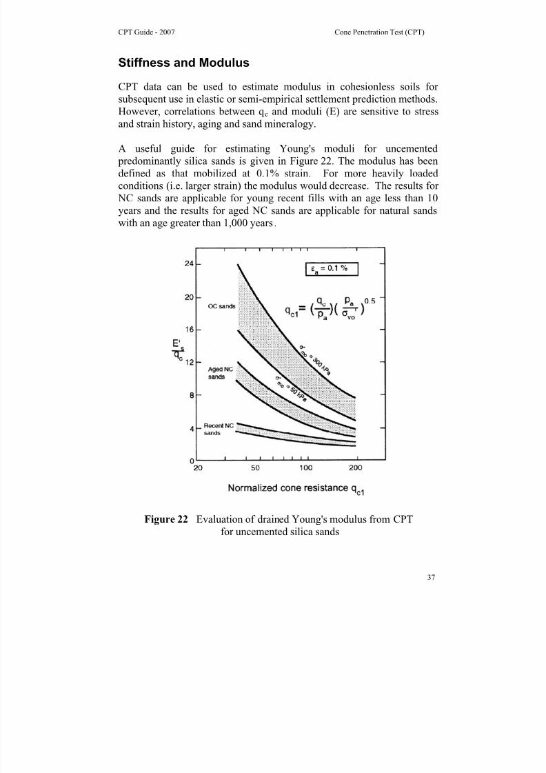
Stiffness and Modulus
CPT data can be used to estimate modulus in cohesionless soils for
subsequent use in elastic or semi-empirical settlement prediction methods.
However, correlations between q c and moduli (E) are sensitive to stress
and strain history, aging and sand mineralogy.
A useful guide for estimating Young's moduli for uncemented
predominantly silica sands is given in Figure 22. The modulus has been
defined as that mobilized at 0.1% strain. For more heavily loaded
conditions (i.e. larger strain) the modulus would decrease. The results for
NC sands are applicable for young recent fills with an age less than 10
years and the results for aged NC sands are applicable for natural sands
with an age greater than 1,000 years.
Figure 22 Evaluation of drained Young's modulus from CPT
for uncemented silica sands

8/13/2019 Cpt Guide Nov 2007 Edition 2
http://slidepdf.com/reader/full/cpt-guide-nov-2007-edition-2 45/126
CPT Guide - 2007 Cone Penetration Test (CPT)
38
Modulus from Shear Wave Velocity
A major advantage of the seismic CPT (SCPT) is the additional
measurement of the shear wave velocity, Vs. The shear wave velocity is
measured using a downhole technique during pauses in the CPT resulting
in a continuous profile of Vs. Elastic theory states that the small strain
shear modulus, Go can be determined from:
Go = ρ Vs2
where ρ is the mass density of the soil (ρ = γ/g).
Hence, the addition of shear wave velocity during the CPT provides a
direct measure of soil stiffness.
The small strain shear modulus represents the elastic stiffness of the soils
at shear strains (γ) less than 10-4
percent. Elastic theory also states that the
small strain Young’s modulus, Eo is linked to Go, as follows;
Eo = 2(1 + υ)Go
Where υ is Poisson’s ratio, which ranges from 0.1 to 0.3 for most soils.
Application to engineering problems requires that the small strainmodulus be softened to the appropriate strain level. For most well
designed structures the degree of softening is often close to a factor of 3.
Hence, for many applications the equivalent Young’s modulus (Es’) can
be estimated from;
Es’ ~ Go = ρ Vs
2
The shear wave velocity can also be used directly for the evaluation of
liquefaction potential. Hence, the seismic CPT provides two independent
methods to evaluate liquefaction potential.

8/13/2019 Cpt Guide Nov 2007 Edition 2
http://slidepdf.com/reader/full/cpt-guide-nov-2007-edition-2 46/126
CPT Guide - 2007 Cone Penetration Test (CPT)
39
Estimating Shear Wave Velocity from CPT
Shear wave velocity can be correlated to CPT cone resistance as a
function of soil type and SBT Ic. Shear wave velocity is sensitive to age
and cementation, where older deposits of the same soil have higher shearwave velocity (i.e. higher stiffness) than younger deposits. Based on
SCPT data, Figure 23 shows a somewhat conservative relationship
between normalized CPT data (Qtn and Fr ) and normalized shear wave
velocity, Vs1, where:
Vs1 = Vs (pa / σ'vo)0.25
Vs1 is in the same units as Vs (e.g. either ft/s or m/s). Younger Holocene
age soils tend to plot toward the center and lower left of the SBT N chart
whereas older Pleistocene age soil tend to plot toward the upper right part
of the chart.
Figure 23 Evaluation of normalized shear wave velocity, Vs1, from CPT
for uncemented Holocene and Pleistocene age soils (1m/s = 3.28 ft/sec)

8/13/2019 Cpt Guide Nov 2007 Edition 2
http://slidepdf.com/reader/full/cpt-guide-nov-2007-edition-2 47/126
CPT Guide - 2007 Cone Penetration Test (CPT)
40
Identification of Unusual Soils Using the SCPT
Almost all available empirical correlations to interpret in-situ tests assume
that the soil is well behaved, i.e. similar to the soils in which the
correlation was based. Many of the existing correlations apply to soilssuch as, unaged, uncemented, silica sands. Application of the existing
empirical correlations in sands other than unaged and uncemented can
produce incorrect interpretations. Hence, it is important to be able to
identify if the soils are ‘well behaved’. The combined measurement of
shear wave velocity and cone resistance provides an opportunity to
identify these ‘unusual’ soils. The cone resistance (q t) is a good measure
of soil strength, since the cone is inducing very large strains and the soil
adjacent to the probe is at failure. The shear wave velocity (Vs) is a direct
measure of the small strain soil stiffness (Go), since the measurement ismade at very small strains. Recent research has shown that unaged and
uncemented sands have data that falls within a narrow range of combined
q t and Go, as shown in Figure 24 and the following equations.
Upper bound, unaged & cemented Go = 280 (q t σ'vo pa)0.3
Lower bound, unaged & cemented Go = 110 (q t σ'vo pa)0.3
Figure 24 Characterization of uncemented, unaged sands(after Eslaamizaad and Robertson, 1997)

8/13/2019 Cpt Guide Nov 2007 Edition 2
http://slidepdf.com/reader/full/cpt-guide-nov-2007-edition-2 48/126
CPT Guide - 2007 Cone Penetration Test (CPT)
41
Hydraulic Conductivity (k)
An approximate estimate of soil hydraulic conductivity or coefficient of
permeability, k , can be made from an estimate of soil behavior type using
the CPT SBT charts. Table 6 provides estimates based on the non-normalized chart shown in Figure 15, while Table 7 provides estimates
based on the normalized chart shown in Figure 16. These estimates are
approximate at best, but can provide a guide to variations of possible
permeability.
Zone Soil Behavior Type (SBT) Range of permeabili ty
k (m/s)
1 Sensitive fine grained 3x10⁻⁹
to 3x10⁻⁸
2 Organic soils 1x10⁻⁸
to 1x10⁻⁶
3 Clay 1x10⁻¹⁰
to 1x10⁻⁹
4 Silty clay to clay 1x10⁻⁹
to 1x10⁻⁸
5 Clayey silt to silty clay 1x10⁻⁸
to 1x10⁻⁷
6 Sandy silt to clayey silt 1x10⁻⁷
to 1x10⁻⁶
7 Silty sand to sandy silt 1x10⁻⁵
to 1x10⁻⁶
8 Sand to silty sand 1x10⁻⁵
to 1x10⁻⁴
9 Sand 1x10⁻⁴
to 1x10⁻³
10 Gravelly sand to dense sand 1x10⁻³
to 1
11 Very stiff fine-grained soil 1x10⁻⁸
to 1x10⁻⁶
12 Very stiff sand to clayey sand 3x10⁻⁷
to 3x10⁻⁴
Table 6 Estimation of soil permeability (k) from the non-normalized
CPT SBT chart by Robertson et al. (1986) shown in Figure 15
Baligh and Levadoux (1980) recommended that the horizontal coefficient
of permeability can be estimated from the expression:
k h = ⎟⎟ ⎠
⎞⎜⎜⎝
⎛
σ
γ
vo
w
'2.3 RR ch
where RR is the re-compression ratio in the overconsolidated range. It
represents the strain per log cycle of effective stress during recompression
and can be determined from laboratory consolidation tests. Baligh and
Levadoux recommended that RR should range from 0.5x10⁻²
to 2x10⁻²
.

8/13/2019 Cpt Guide Nov 2007 Edition 2
http://slidepdf.com/reader/full/cpt-guide-nov-2007-edition-2 49/126
CPT Guide - 2007 Cone Penetration Test (CPT)
42
Zone Soil Behavior Type
(SBTN)
Range of permeabili ty
k (m/s)
1 Sensitive fine grained 3x10⁻⁹
to 3x10⁻⁸
2 Organic soils 1x10⁻⁸
to 1x10⁻⁶
3 Clay 1x10⁻¹⁰
to 1x10⁻⁹
4 Silt mixtures 3x10
-9 to 1x10
-7
5 Sand mixtures 1x10⁻⁷
to 1x10⁻⁵
6 Sands 1x10⁻⁵
to 1x10⁻³
7 Gravelly sands to dense sands 1x10⁻³
to 1
8 Very stiff sand to clayey sand 1x10⁻⁸
to 1x10⁻⁶
9 Very stiff fine-grained soil 1x10⁻⁸
to 1x10⁻⁶
Table 7 Estimation of soil permeability (k) from the normalized CPT
SBT N chart by Robertson (1990) shown in Figure 16
Robertson et al. (1992) presented a summary of available data to estimate
the horizontal coefficient of permeability from dissipation tests, and is
shown in Figure 25. Since the relationship is also a function of the
recompression ratio (RR) there is a wide variation of + or – one order of
magnitude. Jamiolkowski et al. (1985) suggested a range of possible
values of k h /k v for soft clays as shown in Table 8.
Nature of clay k h /k v
No macrofabric, or only slightly developedmacrofabric, essentially homogeneous deposits
1 to 1.5
From fairly well- to well-developed
macrofabric, e.g. sedimentary clays with
discontinuous lenses and layers of more permeable material
2 to 4
Varved clays and other deposits containing
embedded and more or less continuous
permeable layers
3 to 15
Table 8 Range of possible field values of k h/k v for soft clays(after Jamiolkowski et al., 1985)
8/13/2019 Cpt Guide Nov 2007 Edition 2
http://slidepdf.com/reader/full/cpt-guide-nov-2007-edition-2 50/126
CPT Guide - 2007 Cone Penetration Test (CPT)
43
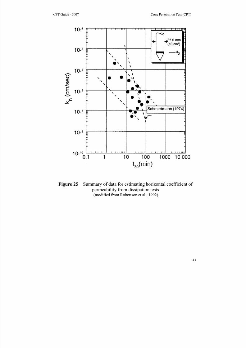
Figure 25 Summary of data for estimating horizontal coefficient of
permeability from dissipation tests(modified from Robertson et al., 1992).

8/13/2019 Cpt Guide Nov 2007 Edition 2
http://slidepdf.com/reader/full/cpt-guide-nov-2007-edition-2 51/126
CPT Guide - 2007 Cone Penetration Test (CPT)
44
Consolidation Characteristics
Flow and consolidation characteristics of a soil are normally expressed in
terms of the coefficient of consolidation, c, and hydraulic conductivity, k .
They are inter-linked through the formula:
c =w
k
γM
where M is the constrained modulus relevant to the problem (i.e.
unloading, reloading, virgin loading).
The parameters c and k vary over many orders of magnitude and are some
of the most difficult parameters to measure in geotechnical engineering.
It is often considered that accuracy within one order of magnitude isacceptable. Due to soil anisotropy, both c and k have different values in
the horizontal (ch , k h) and vertical (cv , k v) direction. The relevant design
values depend on drainage and loading direction.
Details on how to estimate k from CPT soil classification charts are given
in the previous section.
The coefficient of consolidation can be estimated by measuring the
dissipation or rate of decay of pore pressure with time after a stop in CPT penetration. Many theoretical solutions have been developed for deriving
the coefficient of consolidation from CPT pore pressure dissipation data.
The coefficient of consolidation should be interpreted at 50% dissipation,
using the following formula:
c = ⎟⎟ ⎠
⎞⎜⎜⎝
⎛
50
50
t
T r o
2
where:
T50 = theoretical time factor
t50 = measured time for 50% dissipation
r o = penetrometer radius
8/13/2019 Cpt Guide Nov 2007 Edition 2
http://slidepdf.com/reader/full/cpt-guide-nov-2007-edition-2 52/126
CPT Guide - 2007 Cone Penetration Test (CPT)
45
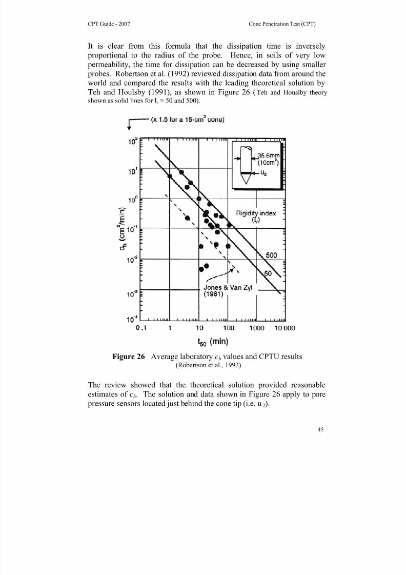
It is clear from this formula that the dissipation time is inversely
proportional to the radius of the probe. Hence, in soils of very low
permeability, the time for dissipation can be decreased by using smaller
probes. Robertson et al. (1992) reviewed dissipation data from around the
world and compared the results with the leading theoretical solution by
Teh and Houlsby (1991), as shown in Figure 26 (Teh and Houslby theory
shown as solid lines for Ir = 50 and 500).
Figure 26 Average laboratory ch values and CPTU results(Robertson et al., 1992)
The review showed that the theoretical solution provided reasonable
estimates of ch. The solution and data shown in Figure 26 apply to pore
pressure sensors located just behind the cone tip (i.e. u2).

8/13/2019 Cpt Guide Nov 2007 Edition 2
http://slidepdf.com/reader/full/cpt-guide-nov-2007-edition-2 53/126
CPT Guide - 2007 Cone Penetration Test (CPT)
46
The ability to estimate ch from CPT dissipation results is controlled by
soil stress history, sensitivity, anisotropy, rigidity index (relative
stiffness), fabric and structure. In overconsolidated soils, the pore
pressure behind the cone tip can be low or negative, resulting in
dissipation data that can initially rise before a decay to the equilibrium
value. Care is required to ensure that the dissipation is continued to the
correct equilibrium and not stopped prematurely after the initial rise. In
these cases, the pore pressure sensor can be moved to the face of the cone
or the t50 time can be estimated using the maximum pore pressure as the
initial value.
Based on available experience, the CPT dissipation method should
provide estimates of ch to within + or – half an order of magnitude.
However, the technique is repeatable and provides an accurate measure ofchanges in consolidation characteristics within a given soil profile.
An approximate estimate of the coefficient of consolidation in the vertical
direction can be obtained using the ratios of permeability in the horizontal
and vertical direction given in the section on hydraulic conductivity,
since:
cv = ch ⎟⎟ ⎠
⎞⎜⎜⎝
⎛
h
v
k k
Table 8 can be used to provide an estimate of the ratio of hydraulic
conductivities.
For short dissipations in sandy soils, the dissipation results can be plotted
on a square-root time scale. The gradient of the initial straight line is m,
where;
ch = (m/MT)2 r 2 (Ir )0.5
MT = 1.15 for u2 position and 10 cm2 cone (i.e. r = 1.78 cm).
8/13/2019 Cpt Guide Nov 2007 Edition 2
http://slidepdf.com/reader/full/cpt-guide-nov-2007-edition-2 54/126
CPT Guide - 2007 Cone Penetration Test (CPT)
47
Constrained Modulus
Consolidation settlements can be estimated using the 1-D Constrained
Modulus, M, where;
M = 1/ mv = δσv / δε
Where mv = equivalent oedometer coefficient of compressibility.
Constrained modulus can be estimated from CPT results using the
following empirical relationship;
M = αM q t
Sangrelat (1970) suggested that αM varies with soil plasticity and natural
water content for a wide range of fine grained soils and organic soils,although the data were based on q c. Meigh (1987) suggested that αM lies
in the range 2 – 8, whereas Mayne (2001) suggested a general value of 8
based on net cone resistance. It is recommended to use an initial value of
αM = 4, unless local experience and/or laboratory test results suggest
higher values.
Estimates of drained 1-D constrained modulus from undrained cone
penetration will be approximate. Estimates can be improved with
additional information about the soil, such as plasticity index and natural
moisture content, where α M is lower for organic soils. Dielectricmeasurements during a CPT can be used to measure in-situ moisture
content in fine grained soils and hence improve the correlation with
constrained modulus.
The same relationship between constrained modulus and cone resistance
applies to sandy soils, where a general value of αM = 4 applies to young,
uncemented, quartz sands. Since, constrained modulus, M, is close to
Young’s modulus (E’) under drained loading, the value for α M varies with
age and stress history (see Figure 22).
8/13/2019 Cpt Guide Nov 2007 Edition 2
http://slidepdf.com/reader/full/cpt-guide-nov-2007-edition-2 55/126
CPT Guide - 2007 Cone Penetration Test (CPT)
48
Appl icat ions o f CPT Results
The previous sections have described how CPT results can be used to
estimate geotechnical parameters which can be used as input in analyses.
An alternate approach is to apply the in-situ test results directly to an
engineering problem. A typical example of this approach is the
evaluation of pile capacity directly from CPT results without the need for
soil parameters.
As a guide, Table 9 shows a summary of the applicability of the CPT for
direct design applications. The ratings shown in the table have been
assigned based on current experience and represent a qualitative
evaluation of the confidence level assessed to each design problem and
general soil type. Details of ground conditions and project requirements
can influence these ratings.
In the following sections a number of direct applications of CPT/CPTU
results are described. These sections are not intended to provide full
details of geotechnical design, since this is beyond the scope of this guide.
However, they do provide some guidelines on how the CPT can be
applied to many geotechnical engineering applications. A good reference
for foundation design is the Canadian Foundation Engineering Manual
(CFEM, 2007, www.bitech.ca).
Type of soil Pile
design
Bearing
capacity
Settlement* Compaction
control
Liquefaction
Sand 1 – 2 1 – 2 2 – 3 1 – 2 1 – 2Clay 1 – 2 1 – 2 3 – 4 3 – 4 1 – 2Intermediate soils 1 – 2 2 – 3 3 – 4 2 – 3 1– 2
Reliability rating: 1=High; 2=High to moderate; 3=Moderate; 4=Moderate to low; 5=low
Table 9 Perceived applicability of the CPT/CPTU for various direct
design problems
(* improves with SCPT data)

8/13/2019 Cpt Guide Nov 2007 Edition 2
http://slidepdf.com/reader/full/cpt-guide-nov-2007-edition-2 56/126
CPT Guide - 2007 Cone Penetration Test (CPT)
49
Shallow Foundation Design
General Design Princip les
Typical Design Sequence:
1. Select minimum depth to protect against:
• external agents: e.g. frost, erosion, trees
• poor soil: fill, organic soils, etc.
2. Define minimum area necessary to protect against soil failure:
• perform bearing capacity analyses
2. Compute settlement and check if acceptable
3. Modify selected foundation if required.
Typical Shallow Foundation Problems
Study of 1200 cases of foundation problems in Europe showed that the
problems could be attributed to the following causes:
• 25% footings on recent fill (mainly poor engineering judgment)
• 20% differential settlement (50% could have been avoided with gooddesign)
• 20% effect of groundwater
• 10% failure in weak layer
• 10% nearby work
(excavations, tunnels, etc.)
• 15% miscellaneous causes
(earthquake, blasting, etc.)
In design, settlement is generally the critical issue. Bearing capacity is
generally not of prime importance.
8/13/2019 Cpt Guide Nov 2007 Edition 2
http://slidepdf.com/reader/full/cpt-guide-nov-2007-edition-2 57/126
CPT Guide - 2007 Cone Penetration Test (CPT)
50
Construct ion
Construction details can significantly alter the conditions assumed in the
design.
Examples are provided in the following list:
• During Excavation
• bottom heave
• slaking, swelling, and softening of expansive clays or rock
• piping in sands and silts
• remolding of silts and sensitive clays
• disturbance of granular soils
• Adjacent construction activity
• groundwater lowering
• excavation
• pile driving
• blasting
• Other effects during or following construction
• reversal of bottom heave
• scour, erosion and flooding
• frost action
8/13/2019 Cpt Guide Nov 2007 Edition 2
http://slidepdf.com/reader/full/cpt-guide-nov-2007-edition-2 58/126
CPT Guide - 2007 Cone Penetration Test (CPT)
51
Shal low Foundat ion - Bearing Capaci ty
General Principles
Load-settlement relationships for typical footings (Vesic, 1972):
1. Approximate elastic response
2. Progressive development of local shear failure
3. General shear failure
In dense granular soils failure typically occurs along a well defined failure
surface. In loose granular soils, volumetric compression dominates and
punching failures are common. Increased depth of overburden can
change a dense sand to behave more like loose sand. In (homogeneous)
cohesive soils, failure occurs along an approximately circular surface.
Significant parameters are:
• nature of soils
• density and resistance of soils
• width and shape of footing
• depth of footing
• position of load.
A given soil does not have a unique bearing capacity; the bearing capacity
is a function of the footing shape, depth and width as well as loadeccentricity.
General Bearing Capacity Theory
Initially developed by Terzaghi (1936); there are now over 30 theories
with the same general form, as follows:
Ultimate bearing capacity, (q f ):
q f = 0.5 γ B Nγ sγ iγ + c Nc sc ic + γ D Nq sq iq
where:
Nγ Nc Nq = Bearing capacity coefficients (function of φ')
sγ sc sq = Shape factors (function of B/L)

8/13/2019 Cpt Guide Nov 2007 Edition 2
http://slidepdf.com/reader/full/cpt-guide-nov-2007-edition-2 59/126
CPT Guide - 2007 Cone Penetration Test (CPT)
52
iγ ic iq = Load inclination factors
B = width of footing
D = depth of footing
L = length of footing
Complete rigorous solutions are impossible since stress fields are
unknown. All theories differ in simplifying assumptions made to write
the equations of equilibrium. No single solution is correct for all cases.
Shape Factors
Shape factors are applied to account for 3-D effects. Based on limited
theoretical ideas and some model tests, recommended factors are as
follows:
sc = sq = 1 + ⎟⎟ ⎠
⎞⎜⎜⎝
⎛ ⎟ ⎠
⎞⎜⎝
⎛
c
q
N
N
L
B
sγ = 1 - 0.4 ⎟ ⎠
⎞⎜⎝
⎛ L
B
Load Inclination Factors
When load is inclined (δ), the shape of a failure surface changes and
reduces the area of failure. Hence, a reduced resistance. At the limit of
inclination, δ = φ, q f = 0, since slippage can occur along the footing-soil
interface.
In general:
ic = iq =2
ο901 ⎟
⎠
⎞⎜⎝
⎛ δ−
ig =
2
1 ⎟⎟ ⎠ ⎞⎜⎜
⎝ ⎛
φδ−
For an eccentric load, Terzaghi proposed a simplified concept of an
equivalent footing width, B'.
B' = B - 2 e

8/13/2019 Cpt Guide Nov 2007 Edition 2
http://slidepdf.com/reader/full/cpt-guide-nov-2007-edition-2 60/126
CPT Guide - 2007 Cone Penetration Test (CPT)
53
where e is the eccentricity. For combined inclined and eccentric load, use
B' and relevant values of shape factors. For footings near a slope, use
modified bearing capacity factors (see Bowles, 1982). They will be small
for clay but large for granular soils.
Effect of Groundwater
The bearing capacity is based on effective stress analyses, hence, position
of the groundwater table affects the value of the soil unit weight.
• If depth to the water table, d w = 0, use γ' in both terms
• If d w = D (depth of footing), use γ' in width term and γ in depth term.
In general, install drainage to keep d w > D.
Indirect Methods Based on Soil Parameters
Granular Soils
Bearing capacity is generally not calculated, since settlements control,
except for very narrow footings.
Cohesive Soils
Short term stability generally controls, hence application of undrainedshear strength, su.
q f = Nc su + γ D
where:
Nc = function of footing width and shape; for strip footings at the ground
surface, Nc = (π + 2).
su = apply Bjerrum’s correction, based on past experience, to field vane
shear strength or from CPT.
Allowable bearing capacity:
q all = (q f - γ D) / FS

8/13/2019 Cpt Guide Nov 2007 Edition 2
http://slidepdf.com/reader/full/cpt-guide-nov-2007-edition-2 61/126
CPT Guide - 2007 Cone Penetration Test (CPT)
54
Hence, q all =FS
Nc us
Where: FS is Factor of Safety, typically = 3.0.
Use a high FS to account for limitations in theory, underestimation of
loads, overestimation of soil strength, avoid local yield in soil and keep
settlements small.
Direct A pp roach to Est im ate Bearing Capaci ty (In-Situ Tests)
Based on in-situ tests, theory, model tests and past foundation
performance.
SPT
• Empirical direct methods
• Limited to granular soils, however, sometimes applied to very stiff clays
• Often linked to allowable settlement of 25mm (Terzaghi & Peck)
• SPT of poor reliability, hence, empirical methods tend to be very
conservative
CPT
Empirical direct methods.
Granular soils:
q f = K φ q c (av)
where:
q c (av) = average CPT penetration resistance below depth of footing, z = B
Eslaamizaad & Robertson (1996) suggested K φ = 0.16 to 0.30 depending
on B/D and shape. In general, assume K φ = 0.16 (see Figure 27).
Meyerhof (1956) suggested K φ = 0.30. However, generally settlements
will control.
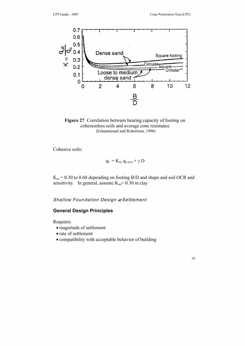
8/13/2019 Cpt Guide Nov 2007 Edition 2
http://slidepdf.com/reader/full/cpt-guide-nov-2007-edition-2 62/126
CPT Guide - 2007 Cone Penetration Test (CPT)
55
Figure 27 Correlation between bearing capacity of footing on
cohesionless soils and average cone resistance(Eslaamizaad and Robertson, 1996)
Cohesive soils:
q f = K su q c (av) + γ D
K su = 0.30 to 0.60 depending on footing B/D and shape and soil OCR and
sensitivity. In general, assume K su= 0.30 in clay
Shal low Foundat ion Design – Settlement
General Design Principles
Requires:
• magnitude of settlement
• rate of settlement
• compatibility with acceptable behavior of building

8/13/2019 Cpt Guide Nov 2007 Edition 2
http://slidepdf.com/reader/full/cpt-guide-nov-2007-edition-2 63/126
CPT Guide - 2007 Cone Penetration Test (CPT)
56
For well designed foundations, the magnitude of strains in the ground is
generally very small (ε < 10-1
%). Hence, ground response is
approximately elastic (non-linear elastic).
Granular Soils
Have high permeability, thus immediate settlements. However, long term
settlements can occur due to submergence, change in water level, blasting,
machine vibration or earthquake loading.
Cohesive Soils
Have very low permeability, thus the need to consider magnitude and
duration of settlement.
In soft, normally to lightly overconsolidated clays, 80% to 90% of
settlement is due to primary consolidation. Secondary settlement also can
be large. In stiff, overconsolidated clays (OCR > 4), approximately 50%
of settlement can be due to immediate distortion settlement and secondary
settlement is generally small.
Methods for Granular Soils
Due to difficulty in sampling, most methods are based on in-situ tests,either direct or via estimate of equivalent elastic modulus (E's).
For most tests, the link between test result and modulus is empirical, since
it depends on many variables; e.g. mineralogy, stress history, stress state,
age, cementation, etc.
SPT
Quick estimates can be made using the simplified chart by Burland et al.
(1977), as shown in Figure 28. The SPT has poor reliability, hence,empirical methods tend to be very conservative.

8/13/2019 Cpt Guide Nov 2007 Edition 2
http://slidepdf.com/reader/full/cpt-guide-nov-2007-edition-2 64/126
CPT Guide - 2007 Cone Penetration Test (CPT)
57
Figure 28 Approximate range of settlement for footings in sand(Burland et al., 1977)
CPT
Meyerhof (1974) suggested that the total settlement, s, could be calculated
using the following formula:
s =c(av)2q
B pΔ
where:
Δ p = net footing pressure
B = footing width
q c (av) = average CPT penetration resistance below depth offooting,
z = B
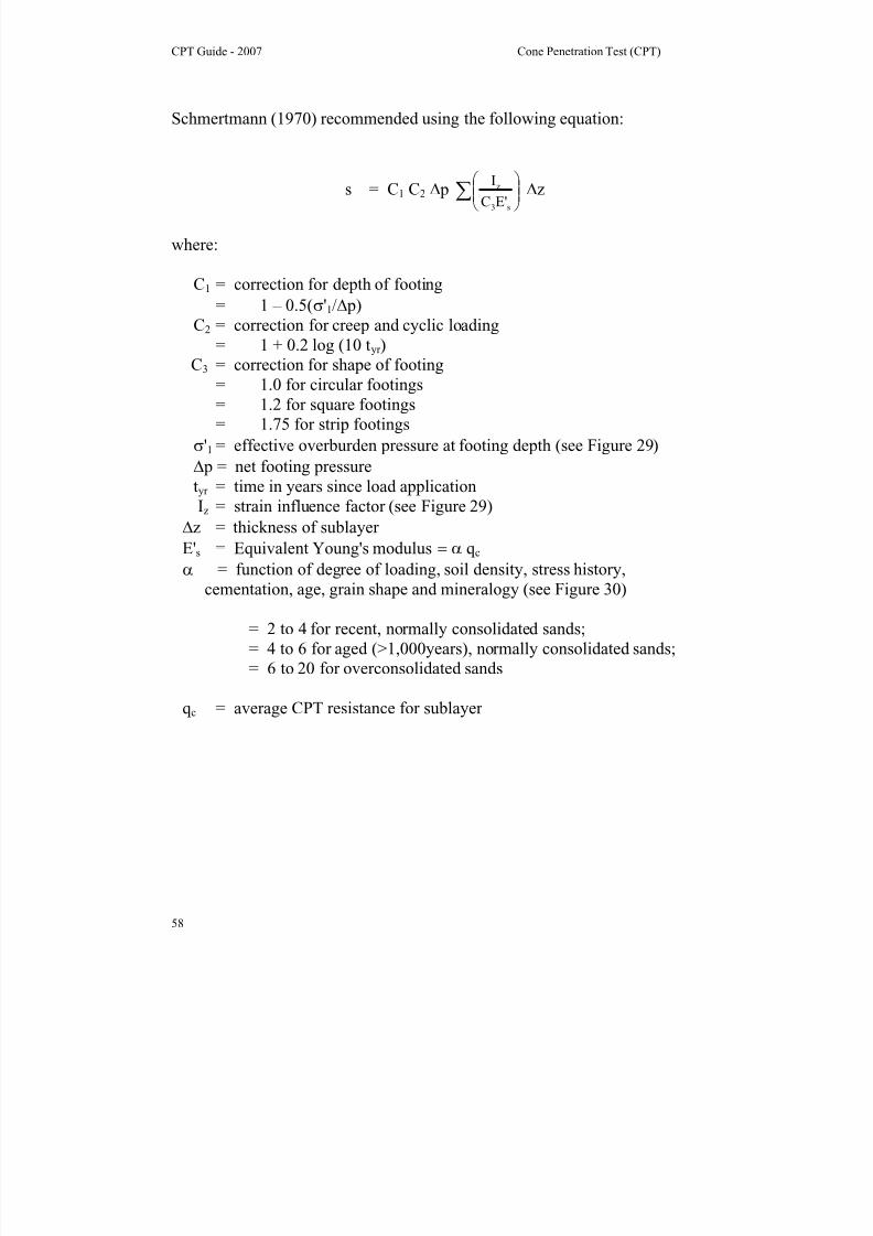
8/13/2019 Cpt Guide Nov 2007 Edition 2
http://slidepdf.com/reader/full/cpt-guide-nov-2007-edition-2 65/126
CPT Guide - 2007 Cone Penetration Test (CPT)
58
Schmertmann (1970) recommended using the following equation:
s = C1 C2 Δ p ∑ ⎟⎟ ⎠
⎞⎜⎜⎝
⎛
s3
z
E'CI Δz
where:
C1 = correction for depth of footing
= 1 – 0.5(σ'1/Δ p)
C2 = correction for creep and cyclic loading
= 1 + 0.2 log (10 tyr )
C3 = correction for shape of footing
= 1.0 for circular footings
= 1.2 for square footings
= 1.75 for strip footings
σ'1 = effective overburden pressure at footing depth (see Figure 29)
Δ p = net footing pressure
tyr = time in years since load application
Iz = strain influence factor (see Figure 29)
Δz = thickness of sublayer
E's = Equivalent Young's modulus = α q c
α = function of degree of loading, soil density, stress history,cementation, age, grain shape and mineralogy (see Figure 30)
= 2 to 4 for recent, normally consolidated sands;
= 4 to 6 for aged (>1,000years), normally consolidated sands;
= 6 to 20 for overconsolidated sands
q c = average CPT resistance for sublayer
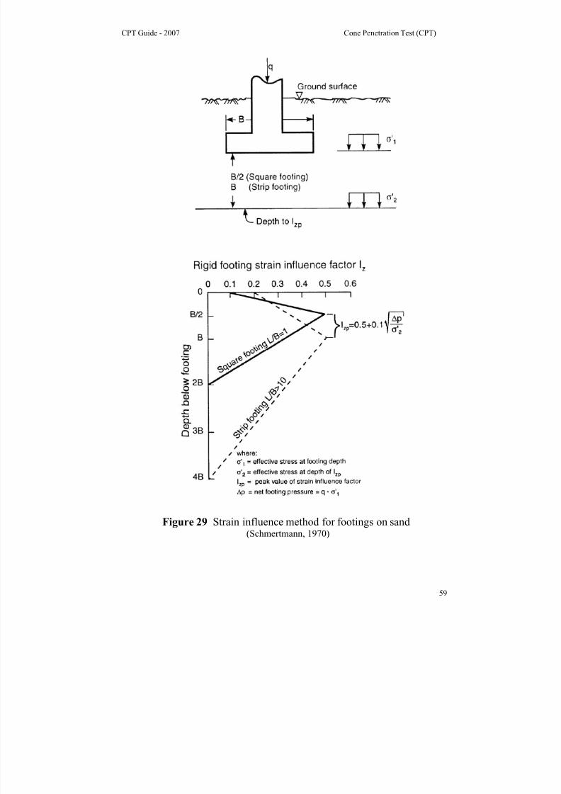
8/13/2019 Cpt Guide Nov 2007 Edition 2
http://slidepdf.com/reader/full/cpt-guide-nov-2007-edition-2 66/126
CPT Guide - 2007 Cone Penetration Test (CPT)
59
Figure 29 Strain influence method for footings on sand(Schmertmann, 1970)

8/13/2019 Cpt Guide Nov 2007 Edition 2
http://slidepdf.com/reader/full/cpt-guide-nov-2007-edition-2 67/126
CPT Guide - 2007 Cone Penetration Test (CPT)
60
Figure 30 Evaluation of drained Young's modulus from CPT
for silica sands(Bellotti et al., 1989)
In this method, (see Figure 31) the sand is divided into a number of layers,
n, of thickness, Δz, down to a depth below the base of the footing equal to
2B for a square footing and 4B for a strip footing (length of footing, L >
10B). A value of q c is assigned to each layer, as illustrated in Figure 31.
Note in sandy soils q c = q t.

8/13/2019 Cpt Guide Nov 2007 Edition 2
http://slidepdf.com/reader/full/cpt-guide-nov-2007-edition-2 68/126
CPT Guide - 2007 Cone Penetration Test (CPT)
61
Figure 31 Application of Schmertmann (1970) method for settlement of
footings on sand
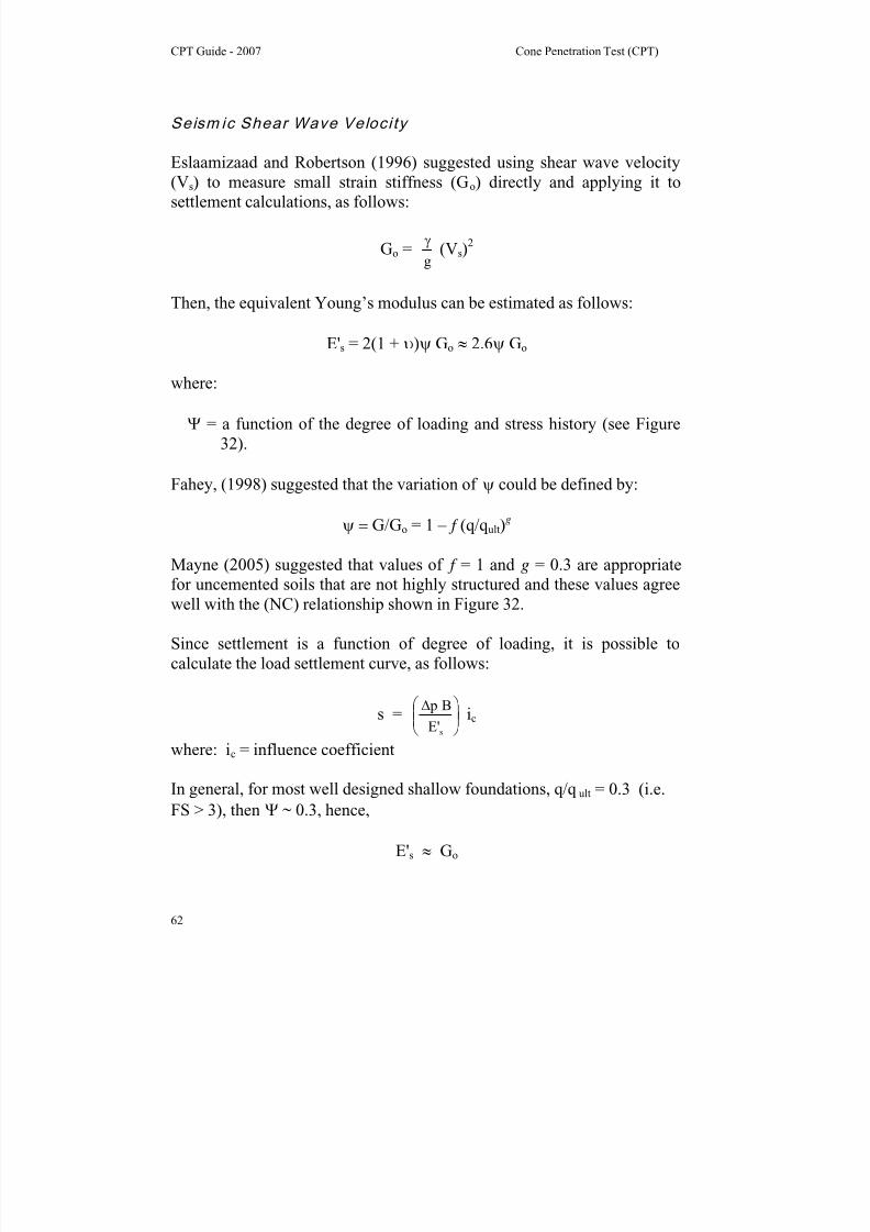
8/13/2019 Cpt Guide Nov 2007 Edition 2
http://slidepdf.com/reader/full/cpt-guide-nov-2007-edition-2 69/126
CPT Guide - 2007 Cone Penetration Test (CPT)
62
Seism ic Shear Wave Veloci ty
Eslaamizaad and Robertson (1996) suggested using shear wave velocity
(Vs) to measure small strain stiffness (Go) directly and applying it tosettlement calculations, as follows:
Go =g
γ (Vs)
2
Then, the equivalent Young’s modulus can be estimated as follows:
E's = 2(1 + υ)ψ Go ≈ 2.6ψ Go
where:
Ψ = a function of the degree of loading and stress history (see Figure
32).
Fahey, (1998) suggested that the variation of ψ could be defined by:
ψ = G/Go = 1 – f (q/q ult)g
Mayne (2005) suggested that values of f = 1 and g = 0.3 are appropriatefor uncemented soils that are not highly structured and these values agree
well with the (NC) relationship shown in Figure 32.
Since settlement is a function of degree of loading, it is possible to
calculate the load settlement curve, as follows:
s = ⎟⎟ ⎠
⎞⎜⎜⎝
⎛ Δ
sE'
B p ic
where: ic = influence coefficient
In general, for most well designed shallow foundations, q/q ult = 0.3 (i.e.
FS > 3), then Ψ ~ 0.3, hence,
E's ≈ Go
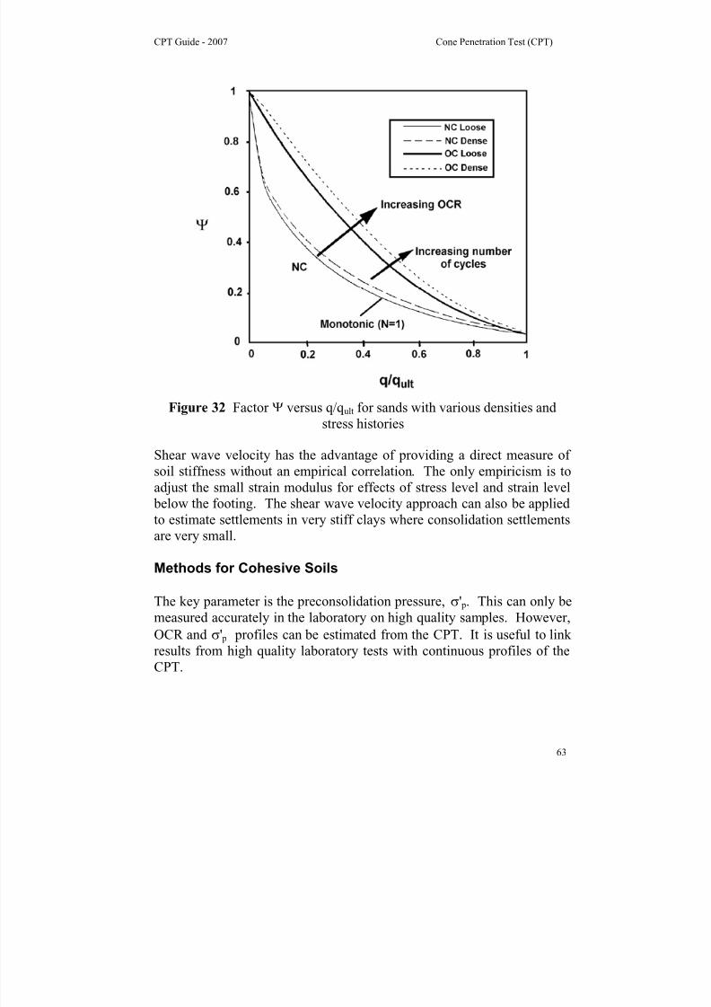
8/13/2019 Cpt Guide Nov 2007 Edition 2
http://slidepdf.com/reader/full/cpt-guide-nov-2007-edition-2 70/126
CPT Guide - 2007 Cone Penetration Test (CPT)
63
Figure 32 Factor Ψ versus q/q ult for sands with various densities and
stress histories
Shear wave velocity has the advantage of providing a direct measure ofsoil stiffness without an empirical correlation. The only empiricism is to
adjust the small strain modulus for effects of stress level and strain level
below the footing. The shear wave velocity approach can also be applied
to estimate settlements in very stiff clays where consolidation settlements
are very small.
Methods for Cohesive Soils
The key parameter is the preconsolidation pressure, σ' p. This can only be
measured accurately in the laboratory on high quality samples. However,
OCR and σ' p profiles can be estimated from the CPT. It is useful to link
results from high quality laboratory tests with continuous profiles of the
CPT.
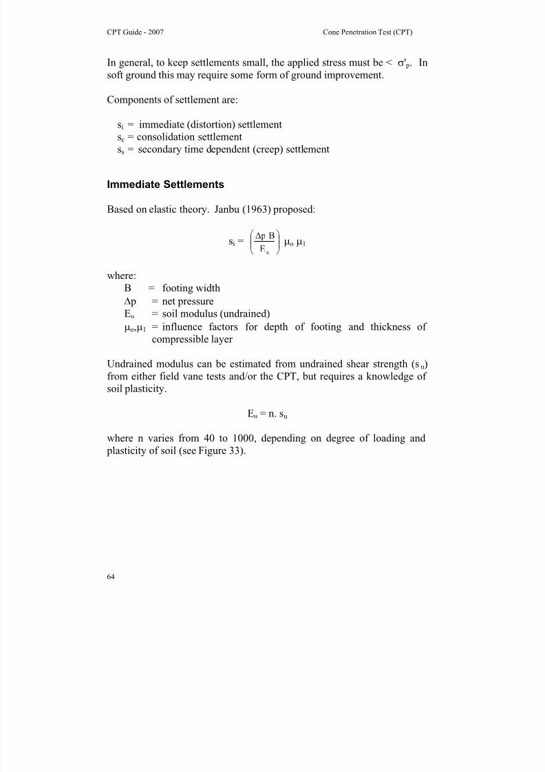
8/13/2019 Cpt Guide Nov 2007 Edition 2
http://slidepdf.com/reader/full/cpt-guide-nov-2007-edition-2 71/126
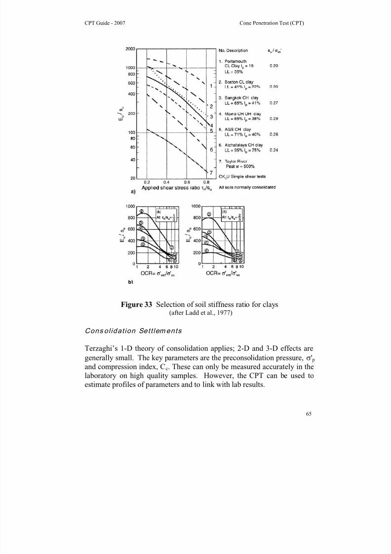
8/13/2019 Cpt Guide Nov 2007 Edition 2
http://slidepdf.com/reader/full/cpt-guide-nov-2007-edition-2 72/126
CPT Guide - 2007 Cone Penetration Test (CPT)
65
Figure 33 Selection of soil stiffness ratio for clays(after Ladd et al., 1977)
Cons ol idat ion Sett lements
Terzaghi’s 1-D theory of consolidation applies; 2-D and 3-D effects are
generally small. The key parameters are the preconsolidation pressure, σ' p
and compression index, Cc. These can only be measured accurately in the
laboratory on high quality samples. However, the CPT can be used to
estimate profiles of parameters and to link with lab results.
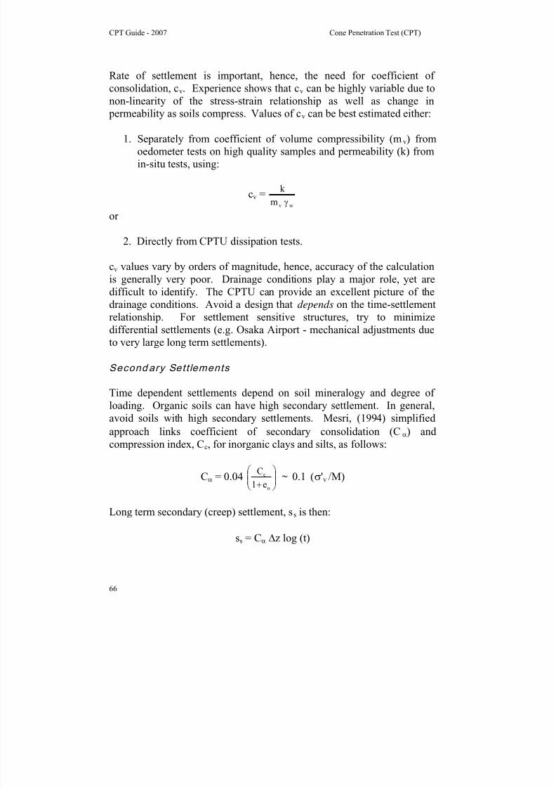
8/13/2019 Cpt Guide Nov 2007 Edition 2
http://slidepdf.com/reader/full/cpt-guide-nov-2007-edition-2 73/126
CPT Guide - 2007 Cone Penetration Test (CPT)
66
Rate of settlement is important, hence, the need for coefficient of
consolidation, cv. Experience shows that cv can be highly variable due to
non-linearity of the stress-strain relationship as well as change in
permeability as soils compress. Values of cv can be best estimated either:
1. Separately from coefficient of volume compressibility (mv) from
oedometer tests on high quality samples and permeability (k) from
in-situ tests, using:
cv =wvm
k
γ
or
2. Directly from CPTU dissipation tests.
cv values vary by orders of magnitude, hence, accuracy of the calculation
is generally very poor. Drainage conditions play a major role, yet are
difficult to identify. The CPTU can provide an excellent picture of the
drainage conditions. Avoid a design that depends on the time-settlement
relationship. For settlement sensitive structures, try to minimize
differential settlements (e.g. Osaka Airport - mechanical adjustments due
to very large long term settlements).
Secondary Sett lements
Time dependent settlements depend on soil mineralogy and degree of
loading. Organic soils can have high secondary settlement. In general,
avoid soils with high secondary settlements. Mesri, (1994) simplified
approach links coefficient of secondary consolidation (Cα) and
compression index, Cc, for inorganic clays and silts, as follows:
Cα = 0.04 ⎟⎟ ⎠
⎞
⎜⎜⎝
⎛
+ o
c
e1
C
~ 0.1 (σ'v /M)
Long term secondary (creep) settlement, ss is then:
ss = Cα Δz log (t)

8/13/2019 Cpt Guide Nov 2007 Edition 2
http://slidepdf.com/reader/full/cpt-guide-nov-2007-edition-2 74/126
CPT Guide - 2007 Cone Penetration Test (CPT)
67
Provided that the applied stress is less than 80% of σ' p, secondary
consolidation is generally small. Constrained Modulus, M can be
estimated from the CPT (see earlier section).
Allowable Settlements
Loads considered in settlement analyses depend on nature of soil and
time-dependence of settlement. Differential settlements generally control.
Sands
• Load: maximum possible load due to immediate settlement
• Differential settlement: can be up to 100% of maximum settlement due
to natural variability of sand. Typically less than or equal to 25mm (1
inch)
Clays
• Load: dead load plus % of live load (LL) depending on duration of
live load
• 50% of LL for buildings
• 30% of LL for bridges
• 75% of LL for reservoirs
• Settlements: are more uniform and can be larger than 25mm (1 inch)
Typical Design Sequence
1. Check for possible isolated footing design
2. Check for possible raft foundation
3. Ground improvement4. Deep foundations

8/13/2019 Cpt Guide Nov 2007 Edition 2
http://slidepdf.com/reader/full/cpt-guide-nov-2007-edition-2 75/126
CPT Guide - 2007 Cone Penetration Test (CPT)
68
Raft Foundations
Consider a raft when:
• Area of footing > 50% of building area• Need to provide underground space in location of high groundwater
• Need to reduce magnitude of total settlements (i.e. floating foundation)
• Need to reduce differential settlements
A raft is an inverted slab, designed to distribute structural loads from
columns and walls, while keeping deformations within acceptable limits.
Structural characteristics of rafts are optimized by accounting for the
interaction between the raft and the supporting ground. Structural
engineers usually perform an elastic analysis using elastic (Winkler)springs. Hence, they would like the spring constant, k s.
k s = coefficient of subgrade reaction (kN/m3)
k s =s
p
where:
p = net applied stress
s = settlement resulting from applied stress, p
The process is governed by the relative stiffness of the structure and the
ground. The coefficient of subgrade reaction is not a soil parameter, since
it depends on the size of the footing and degree of loading. Often
estimates are made from global tables (Terzaghi; see Table 10).

8/13/2019 Cpt Guide Nov 2007 Edition 2
http://slidepdf.com/reader/full/cpt-guide-nov-2007-edition-2 76/126
CPT Guide - 2007 Cone Penetration Test (CPT)
69
Soil type Subgrade reaction
(kN/m3)
Loose sand 5,000 – 16,000
Medium dense sand 10,000 – 80,000
Dense sand 60,000 – 125,000Clayey sand 30,000 – 80,000
Silty sand 20,000 – 50,000
Clayey soil:
su < 50 kPa 10,000 – 20,000
50kPa < su < 100kPa 20,000 – 50,000
100 kPa < su >50,000
Table 10 Recommended coeffiecient of subgrade reaction (k s) for
different soil types (Terzaghi, 1955)
It is best to obtain estimates based on in-situ testing.
Plate Load Tests (PLT)
Provide a direct measure of relationship between p and s, but size effects
can dominate results. Terzaghi (1955) suggested a link between a 1 footsquare plate (k s1) and width of footing B, as follows:
k s = k s1 2
2B
1B⎟ ⎠
⎞⎜⎝
⎛ +
However, there is very large scatter in the results, due to variability in
ground stiffness with depth.

8/13/2019 Cpt Guide Nov 2007 Edition 2
http://slidepdf.com/reader/full/cpt-guide-nov-2007-edition-2 77/126
CPT Guide - 2007 Cone Penetration Test (CPT)
70
Shear Wave Velocity (Vs)
Based on work by Vesic (1961) and elastic theory, the modulus of
subgrade reaction is:
⎟⎟ ⎠
⎞⎜⎜⎝
⎛
ν=
2
s12
f f
4
ss
-1
E
IE
BE65.0k'
where:
Es = modulus of elasticity of soil Es
Ef = modulus of elasticity of footing
B = footing width
If = moment of inertia
ν = Poisson's ratio for soil
k's = modulus of subgrade reaction:
k's = k s B
For most values of Es and Ef , the expression simplifies to:
k's ≈
⎟⎟ ⎠
⎞
⎜⎜⎝
⎛
ν 2
s
-1
E
Bowles (1974) suggested:
k s = 120 q all
where q all is in kPa and k s is in kN/m3.
It is possible to estimate Es from shear wave velocity, Vs. The small strainshear modulus is given by the following:
Go =g
γ(Vs)
2
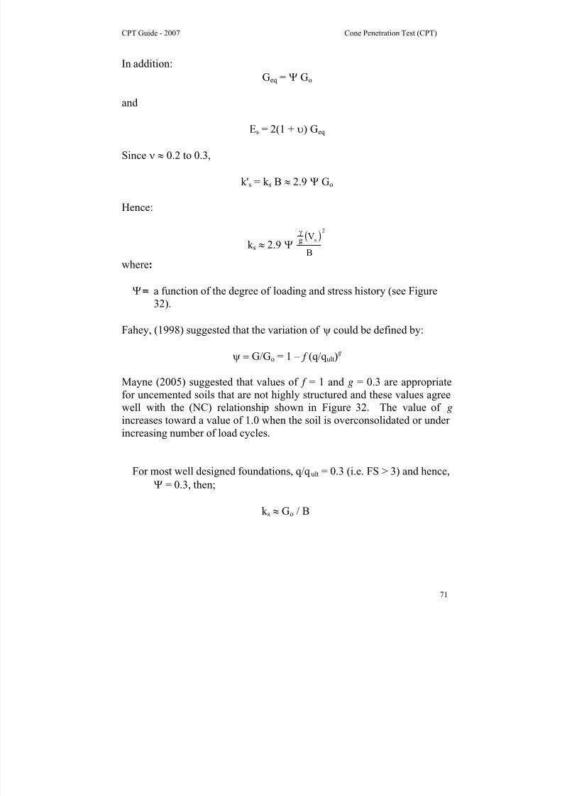
8/13/2019 Cpt Guide Nov 2007 Edition 2
http://slidepdf.com/reader/full/cpt-guide-nov-2007-edition-2 78/126
CPT Guide - 2007 Cone Penetration Test (CPT)
71
In addition:
Geq = Ψ Go
and
Es = 2(1 + υ) Geq
Since ν ≈ 0.2 to 0.3,
k's = k s B ≈ 2.9 Ψ Go
Hence:
k s ≈ 2.9 Ψ ( )
2
s
B
Vg
γ
where:
Ψ a function of the degree of loading and stress history (see Figure
32).
Fahey, (1998) suggested that the variation of ψ could be defined by:
ψ = G/Go = 1 – f (q/q ult)g
Mayne (2005) suggested that values of f = 1 and g = 0.3 are appropriate
for uncemented soils that are not highly structured and these values agree
well with the (NC) relationship shown in Figure 32. The value of g
increases toward a value of 1.0 when the soil is overconsolidated or under
increasing number of load cycles.
For most well designed foundations, q/q ult = 0.3 (i.e. FS > 3) and hence,
Ψ = 0.3, then;
k s ≈ Gο / Β

8/13/2019 Cpt Guide Nov 2007 Edition 2
http://slidepdf.com/reader/full/cpt-guide-nov-2007-edition-2 79/126
CPT Guide - 2007 Cone Penetration Test (CPT)
72
Deep Foundation Design
Piles
Piles can be used to:
• Transfer high surface loads, through soft layers down to stronger
layers
• Transfer loads by friction over significant length of soil
• Resist lateral loads
• Protect against scour, etc.
• Protect against swelling soils, etc
Piles are generally much more expensive than shallow footings.
Types o f Pi les
Generally classified based on installation method (Weltman & Little,
1977):
• Displacement
• Preformed• Driven Cast-in-place
• High pressure grouted
• Non(low)-displacement
• Mud bored
• Cased bored
• Cast-in-place screwed (auger)
Contractors are developing new pile types and installation techniques
constantly to acheive increased capacity and improved cost effectiveness
for different ground conditions. Hence, it is difficult to predict capacity
and load-settlement response for all piles using simple analytical
techniques, since the capacity and load response characteristics can be
dominated by the method of installation.
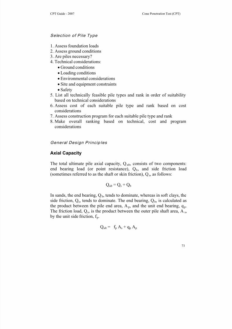
8/13/2019 Cpt Guide Nov 2007 Edition 2
http://slidepdf.com/reader/full/cpt-guide-nov-2007-edition-2 80/126
CPT Guide - 2007 Cone Penetration Test (CPT)
73
Select ion of Pi le Type
1. Assess foundation loads
2. Assess ground conditions3. Are piles necessary?
4. Technical considerations:
• Ground conditions
• Loading conditions
• Environmental considerations
• Site and equipment constraints
• Safety
5. List all technically feasible pile types and rank in order of suitability
based on technical considerations6. Assess cost of each suitable pile type and rank based on cost
considerations
7. Assess construction program for each suitable pile type and rank
8. Make overall ranking based on technical, cost and program
considerations
General Design Princip les
Axial Capacity
The total ultimate pile axial capacity, Qult, consists of two components:
end bearing load (or point resistance), Q b, and side friction load
(sometimes referred to as the shaft or skin friction), Qs, as follows:
Qult = Qs + Q b
In sands, the end bearing, Q b, tends to dominate, whereas in soft clays, the
side friction, Qs, tends to dominate. The end bearing, Q b, is calculated asthe product between the pile end area, A p, and the unit end bearing, q p.
The friction load, Qs, is the product between the outer pile shaft area, A s,
by the unit side friction, f p.
Qult = f p As + q p A p

8/13/2019 Cpt Guide Nov 2007 Edition 2
http://slidepdf.com/reader/full/cpt-guide-nov-2007-edition-2 81/126
CPT Guide - 2007 Cone Penetration Test (CPT)
74
Obviously, different f p values are mobilized along different parts of the
pile, so that, in practice, the calculation is performed as a summation of
small components. For open ended piles, some consideration should be
made regarding whether the pile is plugged or unplugged (de Ruiter and
Beringen, 1979), but the procedure is essentially as outlined above. The
allowable or design pile load, Qall will be then given by the total ultimate
axial capacity divided by a factor of safety. Sometimes separate factors of
safety are applied to Q b and Qs.
Basic approaches are:
• Static Methods
• Pile Dynamics
• Pile Load Tests
Stat ic Methods
Pseudo-theoretical Approach
Pseudo-theoretical methods are based on shear strength parameters.
Similar to bearing capacity calculations for shallow foundations - there
are over 20 different bearing capacity theories. No single solution is
applicable to all piles and most can not account for installation technique.Hence, there has been extensive application of in-situ test techniques
applied via empirical direct design methods.
The most notable is the application of the CPT, since the CPT is a close
model of the pile process. Detailed analysis is generally limited to high-
risk pile design, such as large off-shore piles.
Effect ive Stress App roach ( )
The effective stress (β) approach (Burland, 1973), has been very useful in
providing insight of pile performance.
Unit side friction, f p = β σv’
Unit end bearing, q p = Nt σ b’

8/13/2019 Cpt Guide Nov 2007 Edition 2
http://slidepdf.com/reader/full/cpt-guide-nov-2007-edition-2 82/126
CPT Guide - 2007 Cone Penetration Test (CPT)
75
Soil Type Cast-in-place
Piles
Driven
Piles
Silt 0.2 - 0.3 0.3 - 0.5Loose sand 0.2 - 0.4 0.3 - 0.8
Medium sand 0.3 - 0.5 0.6 - 1.0
Dense sand 0.4 - 0.6 0.8 - 1.2
Gravel 0.4 - 0.7 0.8 - 1.5
Table 11 Range of β coefficients: cohesionless soils
Soil Type Cast-in-place
Piles
Driven
Piles
Silt 10 - 30 20 - 40
Loose sand 20 - 30 30 - 80
Medium sand 30 - 60 50 - 120
Dense sand 50 - 100 100 - 120
Gravel 80 - 150 150 - 300
Table 12 Range of Nt factors: cohesionless soils
The above coefficients are approximate since they depend on ground
characteristics and pile installation details. In the absence of pile load
tests assume FS = 3.
Randolph and Wroth(1982) related β to the overconsolidation ratio (OCR)
for cohesive soils and produced tentative design charts. In general, for
cohesive soils:
β = 0.25 - 0.32, and Nt = 3 - 10
Effective stress concepts may not radically change empirical based design
rules, but can increase confidence in these rules and allow extrapolation to
new situations.

8/13/2019 Cpt Guide Nov 2007 Edition 2
http://slidepdf.com/reader/full/cpt-guide-nov-2007-edition-2 83/126
CPT Guide - 2007 Cone Penetration Test (CPT)
76
Total Stress Appr oach (α )
It has been common to design piles in cohesive soils based on total stressand undrained shear strength, su.
Unit side friction, f p = α su
Unit end bearing, q p = Nt su
Where α varies from 0.5 - 1.0 depending on OCR and Nt varies from 6 to
9 depending on depth of embedment and pile size.
Empir ical App roach
CPT Method
Research has shown (Robertson et al., 1988; Briaud and Tucker, 1988;
Tand and Funegard, 1989; Sharp et al., 1988) that CPT methods generally
give superior predictions of axial pile capacity compared to most
conventional methods. The main reason for this is that the CPT provides a
continuous profile of soil response. Almost all CPT methods usereduction factors to measured CPT values. The need for such reduction
factors is due to a combination of the following influences: scale effect,
rate of loading effects, difference of insertion technique, position of the
CPT friction sleeve and differences in horizontal soil displacements. The
early work by DeBeer (1963) identified the importance of scale effects.
Despite these differences, the CPT is still the test that gives the closest
simulation to a pile. Superiority of CPT methods over non CPT methods
has been confirmed in other studies (e.g. O'Neill, 1986).
The main CPT method by Bustamante and Gianeselli (1982 - LCPCMethod) is outlined below. The LCPC CPT method is recommended
since it provides simple guidance to account for many different pile
installation methods and provides good estimates of axial capacity of
single piles.
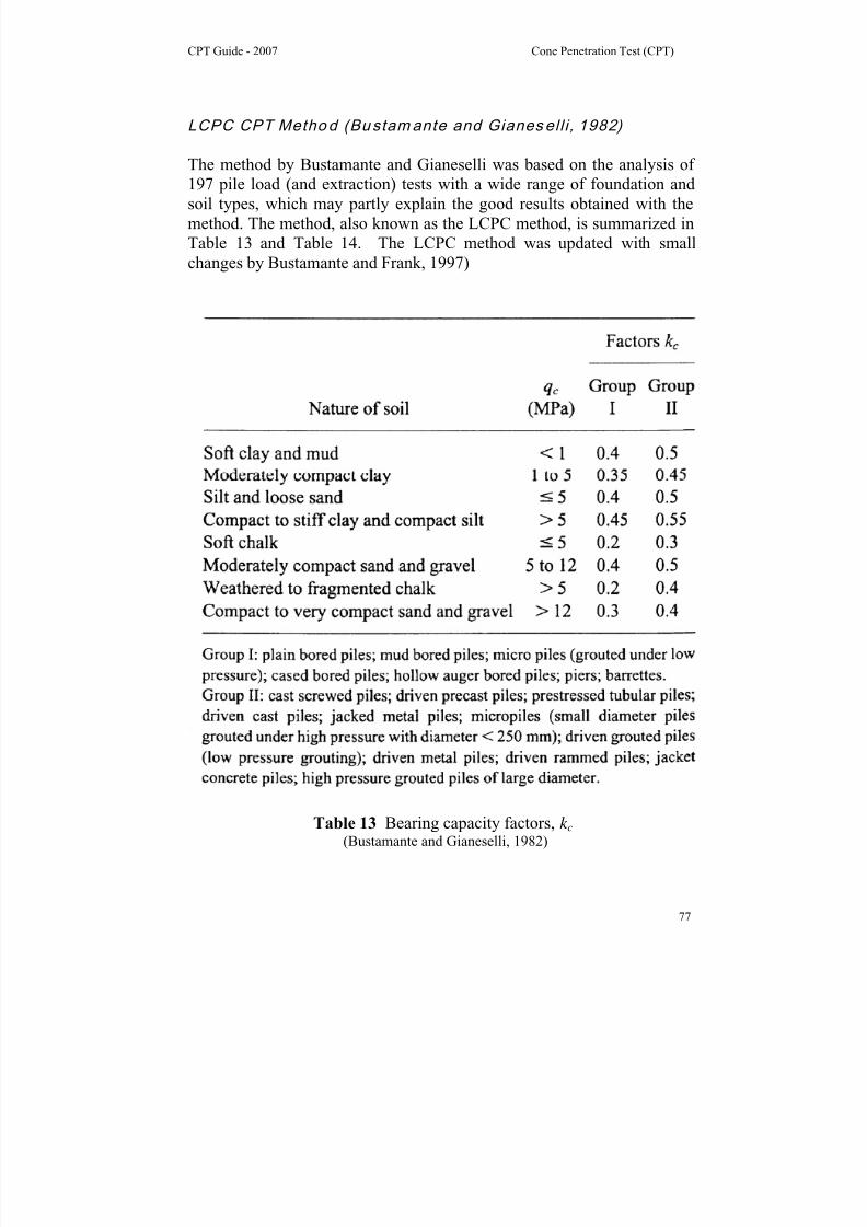
8/13/2019 Cpt Guide Nov 2007 Edition 2
http://slidepdf.com/reader/full/cpt-guide-nov-2007-edition-2 84/126
CPT Guide - 2007 Cone Penetration Test (CPT)
77
LCPC CPT Method (Bustamante and Gianesel l i , 1982)
The method by Bustamante and Gianeselli was based on the analysis of
197 pile load (and extraction) tests with a wide range of foundation andsoil types, which may partly explain the good results obtained with the
method. The method, also known as the LCPC method, is summarized in
Table 13 and Table 14. The LCPC method was updated with small
changes by Bustamante and Frank, 1997)
Table 13 Bearing capacity factors, k c(Bustamante and Gianeselli, 1982)
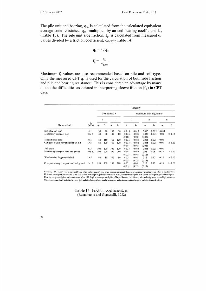
8/13/2019 Cpt Guide Nov 2007 Edition 2
http://slidepdf.com/reader/full/cpt-guide-nov-2007-edition-2 85/126
CPT Guide - 2007 Cone Penetration Test (CPT)
78
The pile unit end bearing, q p, is calculated from the calculated equivalent
average cone resistance, q ca, multiplied by an end bearing coefficient, k c
(Table 13). The pile unit side friction, f p, is calculated from measured q c
values divided by a friction coefficient, αLCPC (Table 14).
q p = k c q ca
f p =LCPC
cq
α
Maximum f p values are also recommended based on pile and soil type.
Only the measured CPT q c is used for the calculation of both side friction
and pile end bearing resistance. This is considered an advantage by many
due to the difficulties associated in interpreting sleeve friction (f s) in CPTdata.
Table 14 Friction coefficient, α(Bustamante and Gianeselli, 1982)
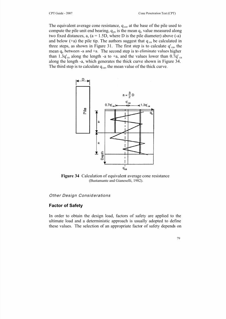
8/13/2019 Cpt Guide Nov 2007 Edition 2
http://slidepdf.com/reader/full/cpt-guide-nov-2007-edition-2 86/126
CPT Guide - 2007 Cone Penetration Test (CPT)
79
The equivalent average cone resistance, q ca, at the base of the pile used to
compute the pile unit end bearing, q p, is the mean q c value measured along
two fixed distances, a, (a = 1.5D, where D is the pile diameter) above (-a)
and below (+a) the pile tip. The authors suggest that q ca be calculated in
three steps, as shown in Figure 31. The first step is to calculate q'ca
, the
mean q c between -a and +a. The second step is to eliminate values higher
than 1.3q'ca along the length -a to +a, and the values lower than 0.7q'ca
along the length -a, which generates the thick curve shown in Figure 34.
The third step is to calculate q ca, the mean value of the thick curve.
Figure 34 Calculation of equivalent average cone resistance(Bustamante and Gianeselli, 1982).
Other Design Consid erations
Factor of Safety
In order to obtain the design load, factors of safety are applied to the
ultimate load and a deterministic approach is usually adopted to define
these values. The selection of an appropriate factor of safety depends on

8/13/2019 Cpt Guide Nov 2007 Edition 2
http://slidepdf.com/reader/full/cpt-guide-nov-2007-edition-2 87/126
CPT Guide - 2007 Cone Penetration Test (CPT)
80
many factors, such as reliability and sufficiency of the site investigation
data, confidence in the method of calculation, previous experience with
similar piles in similar soils and whether or not pile load test results are
available.
Factors of safety are generally of the order of 2, although real values are
sometimes greater, as partial factors of safety are sometimes applied
during calculations (particularly to soil strengths) before arriving to the
ultimate pile capacity.
Recommended factors of safety for calculating the axial capacity of piles
from the CPT are given in Table 15.
Method Factor of safety (FS)
Bustamante and
Gianeselli (1982)2.0 (Qs)
3.0 (Qb)
de Ruiter and Beringen
(1979)2.0 (static loads)
1.5 (static + storm loads)
Table 15 Recommended factors of safety for axial capacity of piles from
CPT
The design of high capacity large diameter bored piles in stiff clay or
dense sand can be difficult due to the fact that settlement criteria usually
control rather than capacity. Hence, very high factors of safety are often
applied to limit settlement.
Pi le Dynam ics
The objective of methods that rely on pile dynamics is to relate the
dynamic pile behavior to the ultimate static pile resistance. Hence, piledynamics can work well in drained soils (sands, gravels, etc.) but can be
difficult in undrained soils (silts, clays, etc.).
The early approach was to use simple pile driving equations (Hiley,
Engineering News, etc.) based on equating the available energy of the
8/13/2019 Cpt Guide Nov 2007 Edition 2
http://slidepdf.com/reader/full/cpt-guide-nov-2007-edition-2 88/126
CPT Guide - 2007 Cone Penetration Test (CPT)
81
hammer to the work performed by the pile. However, these were based
on a rigid pile concept, which is fundamentally incorrect.
Current approaches are based on 1-D wave-equation analyses (Goble et
al., 1970) This method takes into account the characteristics of the;
hammer, driving cap, pile and soil. The method is commonly applied
using commercial software (i.e. WEAP). This method is good to assist in
selection of hammers and prediction of driving stresses and the choice of
driving criteria. It is also useful for dynamic monitoring during
construction.
Pi le Load Tests
Since there is much uncertainty in the prediction of pile capacity and
response, it is common to perform pile load tests on major projects.
For major projects, it is common to apply static methods (i.e. LCPC CPT
method) to obtain a first estimate of capacity, apply pile dynamics if
driven piles selected (aid in hammer selection, driving stresses, driving
criteria) and perform a small number of pile load tests to evaluate pile
response and to calibrate the static method. Results from the pile load
tests can be used to modify the static prediction (i.e. CPT prediction) of
pile capacity and the modified method applied across the site. For low-
risk projects, pile load tests may not be warranted and a slightly
conservative prediction should be applied using the static (CPT) method.
Group Capaci ty
The capacity of a group of piles is influenced by the spacing, pile
installation and ground conditions. The group efficiency is defined as the
ratio of the group capacity to the sum of the individual pile capacities.
Driven piles in cohesionless soils develop larger individual capacities
when installed as a group since lateral earth pressures and soil densityincrease due to pile driving. Hence, it is conservative to use the sum of
the individual pile capacities.
For bored pile groups, the individual capacity can reduce due to reduced
lateral stresses. Meyerhof (1976) suggested a reduction factor of 0.67.

8/13/2019 Cpt Guide Nov 2007 Edition 2
http://slidepdf.com/reader/full/cpt-guide-nov-2007-edition-2 89/126
CPT Guide - 2007 Cone Penetration Test (CPT)
82
For piles in cohesive soils the capacity of the pile group should be
estimated based on the ‘block’ of piles since the soil between the piles
may move with the pile group.
Design of Pi les in Rock
Piles can be placed on or socketed into rock to carry high loads. The
exact area of contact with rock, depth of penetration into rock and quality
of rock are largely unknown, hence, there is much uncertainty. The
capacity is often confirmed based on driving or installation details, local
experience and test loading. End bearing capacity can be based on
pressuremeter test results or strength from rock cores. Shaft resistance
should be estimated with caution, due to possible poor contact between
rock and pile, possible stress concentration and resulting progressivefailure.
Pile Sett lemen t
Although the installation of piles changes the deformation and
compressibility characteristics of the soil mass governing the behavior of
single piles under load, this influence usually extends only a few pile
diameters below the pile base. Meyerhof (1976) suggested that the total
settlement of a group of piles at working load can generally be estimated
assuming an equivalent foundation. For a group of predominately friction piles (i.e. Qs > Q b), the equivalent foundation is assumed to act on the soil
at an effective depth of 2/3 of the pile embedment. For a group of piles
which are predominately end bearing (i.e. Q b > Qs), the equivalent
foundation is taken at or close to the base of the piles. The resulting
settlement is calculated in a manner similar to that of shallow foundations.
Sometimes large capacity piles are installed and used as single piles and
the load settlement response of a single pile is required. The load
settlement response of a single pile is controlled by the combined behavior of the side resistance (Qs) and base resistance (Q b). The side
resistance is usually developed at a small settlement of about 0.5 percent
of the shaft diameter and generally between 5 to 10 mm. In contrast to the
side resistance, the base resistance requires much larger movements to
develop fully, usually about 10 to 20 percent of the base diameter. Hence,
an estimate of the load settlement response of a single pile can be made by
8/13/2019 Cpt Guide Nov 2007 Edition 2
http://slidepdf.com/reader/full/cpt-guide-nov-2007-edition-2 90/126
CPT Guide - 2007 Cone Penetration Test (CPT)
83
combining the two components of resistance according to the above
guidelines. In this way, a friction pile (i.e. Qs >> Q b), will show a clear
plunging failure at a small settlement of about 0.5% of the pile diameter.
On the other hand, an end bearing pile (i.e. Q b >> Qs), will not show a
clear plunging failure until very large settlements have taken place and
usually settlement criteria control before failure can occur. In both cases,
the side friction is almost fully mobilized at working loads. Hence, it is
often important to correctly define the proportions of resistance (Q b/Qs).
Methods have been developed to estimate the load-transfer (t-z) curves
(Verbrugge, 1988). However, these methods are approximate at best and
are strongly influenced by pile installation and soil type. The
recommended method for estimating load settlement response for single
piles is to follow the general guidelines above regarding the development
of each component of resistance.
Negat ive Shaft Fr ict ion and Down Drag on Pi les
When the ground around a pile settles, the resulting downward movement
can induce downward forces on the pile.
The magnitude of the settlement can be very small to develop these
downward forces. For end bearing piles, the negative shaft friction plus
the dead load can result in structural failure of the pile. For friction piles,
the negative shaft friction can result in greater settlements. No pile
subject to down drag will settle more than the surrounding ground.
Lateral Response o f Pi les
Vertical piles can resist lateral loads by deflecting and mobilizing
resistance in the surrounding ground. The response depends on the
relative stiffness of the pile and the ground. In general, the response is
controlled by the stiffness of the ground near the surface, since most long
piles are relatively flexible.
A common approach is to simulate the ground by a series of horizontal
springs. The spring stiffness can be estimated based on a simple subgrade
modulus approach (assumes the ground to be linear and homogeneous) or
as non-linear springs (p-y curves) (Matlock, 1970). The p-y curves can be
8/13/2019 Cpt Guide Nov 2007 Edition 2
http://slidepdf.com/reader/full/cpt-guide-nov-2007-edition-2 91/126
CPT Guide - 2007 Cone Penetration Test (CPT)
84
estimated using empirical relationships based on lab results or in-situ tests
(e.g. pressuremeter, DMT, SCPT) (Baguelin et al., 1978; Robertson et al.,
1986).
Another approach is to simulate the ground as an elastic continuum.
Poulos and Davis, (1980) and Randolph, (1981) suggested design charts
that require estimates of equivalent ground modulus for uniform
homogeneous ground profiles.
The above approaches apply to single piles. When piles are installed in
groups, interaction occurs and lateral deformations can increase. These
can be estimated using simplified theoretical solutions (Poulos and Davis,
1980, Randolph, 1981). The direction of the applied load relative to the
group is important for laterally loaded pile groups.
Liquefaction(see Robertson & Wride, 1998 and Zhang et al., 2002 & 2004 for more details)
Soil liquefaction is a major concern for structures constructed with or on
sand or sandy soils. The major earthquakes of Niigata in 1964 and Kobe
in 1995 have illustrated the significance and extent of damage caused by
soil liquefaction. Soil liquefaction is also a major design problem for
large sand structures such as mine tailings impoundment and earth dams.
To evaluate the potential for soil liquefaction, it is important to determine
the soil stratigraphy and in-situ state of the deposits. The CPT is an ideal
in-situ test to evaluate the potential for soil liquefaction because of its
repeatability, reliability, continuous data and cost effectiveness. This
section presents a summary of the application of the CPT to evaluate soil
liquefaction. Full details are contained in a report prepared for NCEER
(1997) (Youd et al 2001) as a result of a workshop on liquefaction held in
January 1996 and in a paper by Robertson and Wride (1998).
Liqu efact ion Def ini t ions
Several phenomena are described as soil liquefaction, hence, a set of
definitions are provided to aid in the understanding of the phenomena.

8/13/2019 Cpt Guide Nov 2007 Edition 2
http://slidepdf.com/reader/full/cpt-guide-nov-2007-edition-2 92/126
CPT Guide - 2007 Cone Penetration Test (CPT)
85
Flow Liquefaction
• Applies to strain softening soils only (i.e. susceptible to strength loss)
• Requires a strain softening response in undrained loading resulting in
approximately constant shear stress and effective stress• Requires in-situ shear stresses to be greater than the residual or
minimum undrained shear strength
• Either monotonic or cyclic loading can trigger flow liquefaction
• For failure of a soil structure to occur, such as a slope, a sufficient
volume of material must strain soften. The resulting failure can be a
slide or a flow depending on the material characteristics and ground
geometry. The resulting movements are due to internal causes and can
occur after the trigger mechanism occurs
• Can occur in any metastable saturated soil, such as very loose fine
cohesionless deposits, very sensitive clays, and loess (silt) deposits
Cyclic (softening) Liquefaction
• Requires undrained cyclic loading during which shear stress reversal
occurs or zero shear stress can develop
• Requires sufficient undrained cyclic loading to allow effective stresses
to reach essentially zero
• Deformations during cyclic loading can accumulate to large values,
but generally stabilize shortly after cyclic loading stops. The resultingmovements are due to external causes and occur mainly during the
cyclic loading
• Can occur in almost all saturated sands provided that the cyclic loading
is sufficiently large in magnitude and duration
• Clayey soils can experience cyclic softening when the applied cyclic
shear stress is close to the undrained shear strength. Deformations are
generally small due to the cohesive strength at low effective stress.
Rate effects (creep) often control deformations in cohesive soils.
Note that strain softening soils can also experience cyclic liquefaction
depending on ground geometry. Figure 35 presents a flow chart
(Robertson and Wride, 1998) to clarify the phenomena of soil
liquefaction.
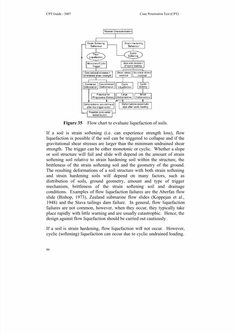
8/13/2019 Cpt Guide Nov 2007 Edition 2
http://slidepdf.com/reader/full/cpt-guide-nov-2007-edition-2 93/126
CPT Guide - 2007 Cone Penetration Test (CPT)
86
Figure 35 Flow chart to evaluate liquefaction of soils.
If a soil is strain softening (i.e. can experience strength loss), flow
liquefaction is possible if the soil can be triggered to collapse and if the
gravitational shear stresses are larger than the minimum undrained shear
strength. The trigger can be either monotonic or cyclic. Whether a slope
or soil structure will fail and slide will depend on the amount of strain
softening soil relative to strain hardening soil within the structure, the
brittleness of the strain softening soil and the geometry of the ground.
The resulting deformations of a soil structure with both strain softening
and strain hardening soils will depend on many factors, such as
distribution of soils, ground geometry, amount and type of trigger
mechanism, brittleness of the strain softening soil and drainage
conditions. Examples of flow liquefaction failures are the Aberfan flow
slide (Bishop, 1973), Zealand submarine flow slides (Koppejan et al.,
1948) and the Stava tailings dam failure. In general, flow liquefactionfailures are not common, however, when they occur, they typically take
place rapidly with little warning and are usually catastrophic. Hence, the
design against flow liquefaction should be carried out cautiously.
If a soil is strain hardening, flow liquefaction will not occur. However,
cyclic (softening) liquefaction can occur due to cyclic undrained loading.
8/13/2019 Cpt Guide Nov 2007 Edition 2
http://slidepdf.com/reader/full/cpt-guide-nov-2007-edition-2 94/126
8/13/2019 Cpt Guide Nov 2007 Edition 2
http://slidepdf.com/reader/full/cpt-guide-nov-2007-edition-2 95/126
CPT Guide - 2007 Cone Penetration Test (CPT)
88
where τav is the average cyclic shear stress; amax is the maximum
horizontal acceleration at the ground surface; g is the acceleration due to
gravity; σvo and σ'vo are the total and effective vertical overburden
stresses, respectively; and r d is a stress reduction factor which is
dependent on depth. The factor r d can be estimating using the followingtri-linear function, which provides a good fit to the average of the
suggested range in r d originally proposed by Seed and Idriss (1971):
r d = 1.0 – 0.00765z
if z < 9.15 m
= 1.174 – 0.0267z
if z = 9.15 to 23 m
= 0.744 – 0.008zif z = 23 to 30 m
= 0.5
if z > 30 m
where z is the depth in meters. These formulae are approximate at best
and represent only average values since r d shows considerable variation
with depth. Recently Idriss has suggested alternate values for r d , but these
are associated with alternate values of CRR and are not recommended.
The sequence to evaluate cyclic liquefaction for level ground sites is:
1. Evaluate susceptibility to cyclic liquefaction
2. Evaluate triggering of cyclic liquefaction
3. Evaluate post-earthquake deformations.
1. Evaluate Susceptibil ity to Cycli c L iquefaction
The response of soil to seismic loading varies with soil type and state
(void ratio, effective confining stress, stress history, etc.). Boulanger andIdriss (2004) correctly distinguished between sand-like and clay-like
behavior. The following criteria can be used to identify soil behavior:
Sand-like Behavior
Sand-like soils are susceptible to cyclic liquefaction when their behavior
is characterized by Plasticity Index (PI) < 12 and Liquid Limit (LL) < 37
8/13/2019 Cpt Guide Nov 2007 Edition 2
http://slidepdf.com/reader/full/cpt-guide-nov-2007-edition-2 96/126
CPT Guide - 2007 Cone Penetration Test (CPT)
89
and natural water content (wc) > 0.8 (LL). More emphasis should be
placed on PI, since both LL and wc tend to be less reliable.
• Low risk project: Assume soils are susceptible to cyclic
liquefaction unless previous local experience shows otherwise.
• High risk project: Either assume soils are susceptible to cyclicliquefaction or obtain high quality samples and evaluate
susceptibility based on appropriate laboratory testing, unless
previous local experience exists.
Clay-like Behavior
Clay-like soils are generally not susceptible to cyclic liquefaction when
their behavior is characterized by PI > 12 but they can experience cyclic
softening.
• Low risk project: Assume soils are not susceptible to cyclic
liquefaction unless previous local experience shows otherwise.Check for cyclic softening.
• High risk project: Obtain high quality samples and evaluate
susceptibility to either cyclic liquefaction and/or cyclic softening
based on appropriate laboratory testing, unless previous local
experience exists.
These criteria are generally conservative. Boulanger and Idriss (2004)
suggested that sand-like behavior is limited to PI < 7. Use the above
criteria, unless local experience in the same geology unit shows that alower PI is more appropriate.
2. Evaluate Tr igger ing of Cyclic L iquefaction
Sand-li ke Mater ials
Seed et al., (1985) developed a method to estimate the cyclic resistance
ratio (CRR) for clean sand with level ground conditions based on the
Standard Penetration Test (SPT). Recently the CPT has become more
popular to estimate CRR, due to the continuous, reliable and repeatable
nature of the data (NCEER, 1997; Youd et al., 2001) and a larger data base.
Apply the simplified (NCEER) approach as described by Youd et al
(2001) using generally conservative assumptions. The simplified
approach should be used for low to medium risk projects and for
preliminary screening for high risk projects. For low risk projects, where

8/13/2019 Cpt Guide Nov 2007 Edition 2
http://slidepdf.com/reader/full/cpt-guide-nov-2007-edition-2 97/126
CPT Guide - 2007 Cone Penetration Test (CPT)
90
the simplified approach is the only method applied, conservative criteria
should be used. The recommended CPT correlation for clean sand is
shown in Figure 36 and can be estimated using the following simplified
equations:
CRR 7.5 =( )
08.01000
q 93
3
cs N1c +⎥⎦
⎤⎢⎣
⎡
if 50 ≤ (q c1N)cs ≤ 160
CRR 7.5 =( )
05.01000
q 833.0
3
cs N1c +⎥⎦
⎤⎢⎣
⎡
if (q c1N)cs < 50
The field observations used to compile the curve in Figure 33 are based
primarily on the following conditions:
• Holocene age, clean sand deposits
• Level or gently sloping ground
• Magnitude M = 7.5 earthquakes• Depth range from 1 to 15 m ( 3 to 45 feet) (85% is for depths < 10 m
(30 ft)
• Representative average CPT values for the layer considered to have
experienced cyclic liquefaction.
Caution should be exercised when extrapolating the CPT correlation to
conditions outside the above range. An important feature to recognize is
that the correlation is based primarily on average values for the inferred
liquefied layers. However, the correlation is often applied to all measured
CPT values, which include low values below the average. Therefore, the
correlation can be conservative in variable deposits where a small part of
the CPT data can indicate possible liquefaction.
8/13/2019 Cpt Guide Nov 2007 Edition 2
http://slidepdf.com/reader/full/cpt-guide-nov-2007-edition-2 98/126
CPT Guide - 2007 Cone Penetration Test (CPT)
91
Figure 36 Cyclic resistance ratio (CRR) from CPT for clean sands(After Robertson and Wride, 1998)
It has been recognized for some time that the correlation to estimate
CRR 7.5 for silty sands is different than that for clean sands. Typically a
correction is made to determine an equivalent clean sand penetration
resistance based on grain characteristics, such as fines content, althoughthe corrections are due to more than just fines content and are influenced
by the plasticity of the fines.
One reason for the continued use of the SPT has been the need to obtain a
soil sample to determine the fines content of the soil. However, this has
been offset by the generally poor repeatability of the SPT data. It is now

8/13/2019 Cpt Guide Nov 2007 Edition 2
http://slidepdf.com/reader/full/cpt-guide-nov-2007-edition-2 99/126
CPT Guide - 2007 Cone Penetration Test (CPT)
92
possible to estimate grain characteristics directly from the CPT.
Robertson and Wride (R&W, 1998) suggest estimating an equivalent
clean sand cone penetration resistance, (q c1N)cs (or more recently, (Qtn)cs )
using the following:
(q c1N)cs = K c (q c1N) = K c Qtn
where K c is a correction factor that is a function of grain characteristics
(combined influence of fines content and plasticity)of the soil.
Robertson and Wride (1998) suggest estimating the grain characteristics
using the soil behavior chart by Robertson (1990) and the soil behavior
type index, Ic, where:
Ic = ( ) ( )[ ]5.022 22.1FlogQlog47.3 ++−
and Qtn =
n
vo
a
2a
voc
'
P
P
q ⎟⎟ ⎠
⎞⎜⎜⎝
⎛
σ⎟⎟ ⎠
⎞⎜⎜⎝
⎛ σ−
is the normalized CPT penetration resistance (dimensionless); n = stress
exponent; F = f s/[(q c - σvo)] x 100% is the normalized friction ratio (in
percent); f s is the CPT sleeve friction stress; σvo and σ'vo are the total
effective overburden stresses respectively; Pa is a reference pressure in thesame units as σ'vo (i.e. Pa = 100 kPa if σ'vo is in kPa) and Pa2 is a reference
pressure in the same units as q c and σvo (i.e. Pa2 = 0.1 MPa if q c and σvo
are in MPa). Note, 1 tsf ~ 0.1 MPa.
The soil behavior type chart by Robertson (1990) (see Figure 16) uses a
normalized cone penetration resistance (Qt) based on a simple linear stress
exponent of n = 1.0 (see above), whereas the chart recommended here for
estimating CRR is essentially based on a normalized cone penetration
resistance (q c1N) based on a stress exponent n = 0.5. Olsen and Malone
(1988) correctly suggested a normalization where the stress exponent (n)varies from around 0.5 in sands to 1.0 in clays. However, this
normalization for soil type is somewhat complex and iterative.
The Robertson (1990) procedure using n = 1.0 (i.e. Qt) is recommended
for soil classification in clay type soils when Ic > 2.6. However, in sandy

8/13/2019 Cpt Guide Nov 2007 Edition 2
http://slidepdf.com/reader/full/cpt-guide-nov-2007-edition-2 100/126
CPT Guide - 2007 Cone Penetration Test (CPT)
93
soils when Ic ≤ 2.6, it is recommended that data being plotted on the
Robertson (1990) chart be modified by using n = 0.5. Hence, the
recommended procedure is to first use n = 1.0 to calculate Qt and,
therefore, an initial value of Ic for CPT data. If Ic > 2.6, the data should be
plotted directly on the Robertson (1990) chart (and assume q c1N = Qt).However, if Ic ≤ 2.6, the exponent to calculate Qt should be changed to n
= 0.5 and Ic should be recalculated based on q c1N and F. If the
recalculated Ic remains less than 2.6, the data should be plotted on the
Robertson (1990) chart using q c1N based on n = 0.5. If, however, Ic
iterates above and below a value of 2.6, depending which value of n is
used, a value of n = 0.75 should be selected to calculate q c1N and plot data
on the Robertson (1990) chart. Note that if the in-situ effective
overburden stresses are in the order of 50 kPa to 150 kPa, the choice of
normalization has little effect on the calculated normalized penetration
resistance. Zhang, Robertson and Brachman (2002 and 2004) updatedthe procedure to estimate the stress exponent ‘n’ as a function of the CPT
soil behavior type, Ic (see Figure 37).
The recommended relationship between Ic and the correction factor K c is
given by the following:
K c = 1.0 if Ic ≤ 1.64
K c = - 0.403 Ic
4
+ 5.581 Ic
3
– 21.63 Ic
2
+ 33.75 Ic – 17.88 if Ic > 1.64
The correction factor, K c, is approximate since the CPT responds to many
factors such as soil plasticity, fines content, mineralogy, soil sensitivity,
age, and stress history. However, in general, these same factors influence
the CRR 7.5 in a similar manner. Caution should be used when applying
the relationship to sands that plot in the region defined by 1.64 < Ic < 2.36
and F < 0.5% so as not to confuse very loose clean sands with sands
containing fines. In this zone, it is suggested to set K c = 1.0. Soils with Ic
> 2.6 (and F > 1%) fall into the clay-like regions of the CPT soil behavior
chart and, in general, are not susceptible to cyclic liquefaction. However,samples should be obtained and liquefaction potential evaluated using
other criteria based primarily on plasticity, e.g. soils with plasticity index
greater than 12 are likely not susceptible to liquefaction. Soils that fall in
the lower left region of the CPT soil behavior chart defined by Ic > 2.6 but
F < 1.0% can be sensitive and hence, possibly susceptible to both cyclic

8/13/2019 Cpt Guide Nov 2007 Edition 2
http://slidepdf.com/reader/full/cpt-guide-nov-2007-edition-2 101/126
CPT Guide - 2007 Cone Penetration Test (CPT)
94
and flow liquefaction. The full methodology to estimate CRR 7.5 from the
CPT is summarized in Figure 37.
For low risk projects and for preliminary screening in high risk projects,
Robertson and Wride (1998) suggested that when Ic > 2.6 and F > 1% the
soil would have clay-like behavior and would likely not be susceptible to
liquefaction. Youd et al (2001) recommends that soils be sampled where
Ic > 2.4 to verify the behavior type. When Ic > 2.4 selected (disturbed)
soil samples (for grain size distribution, Atterberg limits and water
content) should be obtained and tested to confirm susceptibility to cyclic
liquefaction using the criteria in the previous section. Selective soil
sampling based on Ic should be carried out adjacent to some CPT
soundings. Disturbed samples can be obtained using either direct push
samplers (using CPT equipment) or conventional drilling/sampling
techniques close to the CPT sounding.
The factor of safely against cyclic liquefaction is defined as:
Factor of Safety, FS =CSR
CRR5.7 MSF
Where:
MSF is the Magnitude Scaling Factor to convert the CRR 7.5 for M =
7.5 to the equivalent CRR for the design earthquake.
The recommended MSF is given by:
MSF =56.2M
174
The above recommendations are based on the NCEER Workshop in 1996(NCEER, 1997 and Youd et al., 2001)
Juang et al., (2006) related Factor of Safety (FS) to the probability of
liquefaction (PL) for the R&W CPT Methods using:
PL = 1 / (1 + (FS/0.81)5.45
)
8/13/2019 Cpt Guide Nov 2007 Edition 2
http://slidepdf.com/reader/full/cpt-guide-nov-2007-edition-2 102/126
CPT Guide - 2007 Cone Penetration Test (CPT)
95
if Ic <= 1.64, Kc = 1.0
if 1.64< Ic < 2.60, Kc = -0.403I c4 + 5.581 I c
3 – 21.63 I c
2 + 33.75 Ic – 17.88
if Ic >= 2.60, evaluate using other criteria; likely non- liquefiable if F > 1%
BUT , if 1.64 < Ic < 2.36 and F < 0.5%, set Kc = 1.0
08 . 0 1000
) ( 93
3
1
5 . 7 + ⎟ ⎜ ⎝
⎛ ⋅ =
cs N cq CRR , if 50 <= (q c1N)cs < 160
05 . 0 1000
) ( 833 . 0
1
5 . 7 + ⎟ ⎜ ⎝
⎛ ⋅ =
cs N cq CRR , if (qc1N)cs < 50
if Ic >= 2.60, evaluate using other criteria; likely non- liquefiable if F > 1%
Q K q ccs N c ⋅ = ) ( 1
q c : tip resistance, f s : sleeve friction
σ vo , σ vo’ : in-situ vertical total and effective stress
units: all in kPa
initial stress exponent : n = 1.0 and calcualte Q, F, and Ic
if Ic <= 1.64, n = 0.5
if 1.64 < Ic < 3.30, n = ( Ic –1.64)*0.3 + 0.5
if Ic >= 3.30, n = 1.0
iterate until the change in n, Δ n < 0.01
if σ vo’ > 300 kPa, let n = 1.0 for all soils
n
vo
nC ⎟ ⎟
⎜ ⎜
⎝
⎛ =
'
100
σ
n
voc C
q Q ⋅
− =
100
) ( σ , 100
) ( ⋅
− =
voc
s
q F
σ
[ ]22) log 22 . 1 ( ) log 47 . 3 ( F Q I c + + − =
Figure 37 Flow chart to evaluate cyclic resistance ratio from CPT(Updated from Robertson and Wride, 1998)
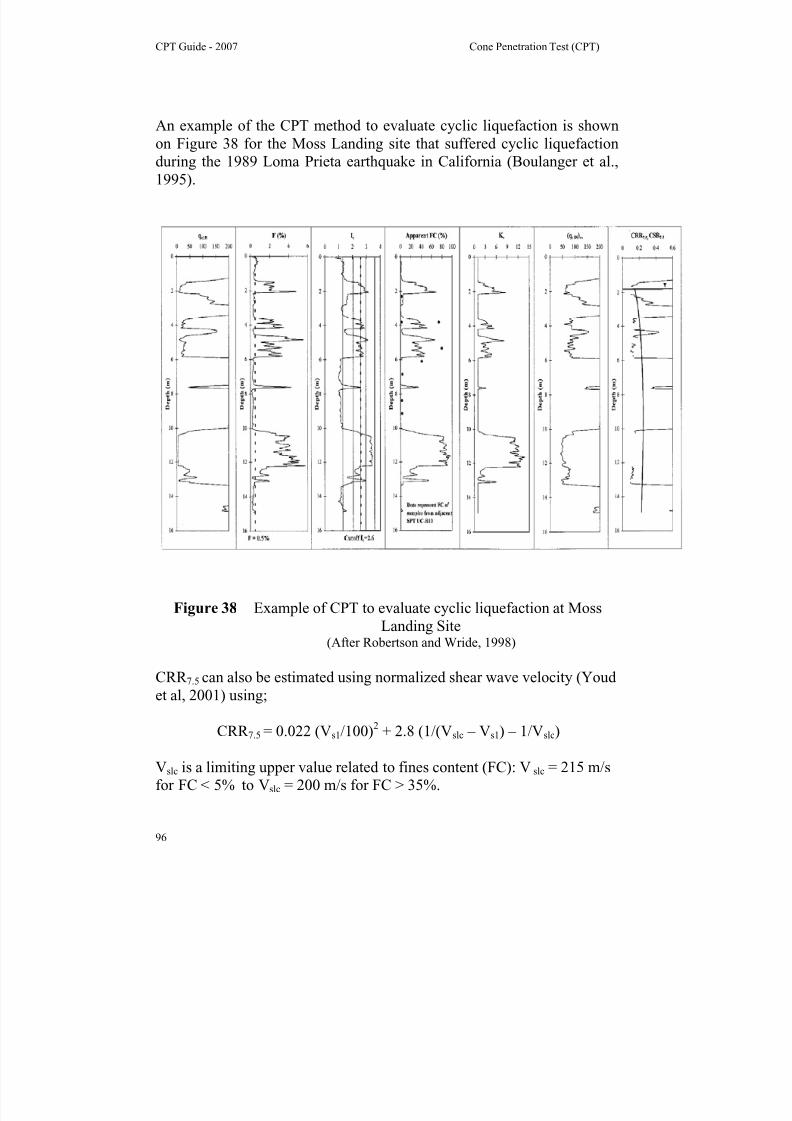
8/13/2019 Cpt Guide Nov 2007 Edition 2
http://slidepdf.com/reader/full/cpt-guide-nov-2007-edition-2 103/126
CPT Guide - 2007 Cone Penetration Test (CPT)
96
An example of the CPT method to evaluate cyclic liquefaction is shown
on Figure 38 for the Moss Landing site that suffered cyclic liquefaction
during the 1989 Loma Prieta earthquake in California (Boulanger et al.,
1995).
Figure 38 Example of CPT to evaluate cyclic liquefaction at Moss
Landing Site(After Robertson and Wride, 1998)
CRR 7.5 can also be estimated using normalized shear wave velocity (Youdet al, 2001) using;
CRR 7.5 = 0.022 (Vs1/100)2 + 2.8 (1/(Vslc – Vs1) – 1/Vslc)
Vslc is a limiting upper value related to fines content (FC): Vslc = 215 m/s
for FC < 5% to Vslc = 200 m/s for FC > 35%.
8/13/2019 Cpt Guide Nov 2007 Edition 2
http://slidepdf.com/reader/full/cpt-guide-nov-2007-edition-2 104/126
CPT Guide - 2007 Cone Penetration Test (CPT)
97
Clay-like Mater ials
Because of the cohesive nature of clay-like materials, they develop much
smaller pore pressures under undrained cyclic loading than sand-like
materials. Hence, clay-like materials do not reach zero effective stress
with resulting large deformations under cyclic loading. Hence, clay-like
materials are not susceptible to cyclic liquefaction. However, when the
cyclic stress ratio (CSR) is large relative to the undrained shear strength
ratio of clay-like materials, deformations can develop. Boulanger and
Idriss (2007) used the term ‘cyclic softening’ to define this build-up of
deformations under cyclic loading in clay-like soils. Boulanger and Idriss
(2007) showed that the CRR for cyclic softening in clay-like materials is
controlled by the undrained shear strength ratio, which in term is
controlled by the stress history (OCR). Boulanger and Idriss (2007)
recommended the following expressions for CRR M=7.5 (for a magnitude7.5 earthquake) in natural deposits of clay-like soils:
CRR M=7.5 = 0.8 (su/σ'vc) K α
and
CRR M=7.5 = 0.18 (OCR)0.8
K α
Where:
Su/σ’vc is the undrained shear strength ratio for the appropriate direction of
loading.K α is a correction factor to account to static shear stress. For well
designed structures where the factor of safety for static loading is large,
K α is generally close to 0.9.
For seismic loading where CSR < 0.6, cyclic softening is possible only in
normally to lightly overconsolidated (OCR < 4) clay-like soils.
Boulanger and Idriss (2007) recommended three approaches to determine
CRR for clay-like materials, which are essentially:
1. Estimate using empirical methods based on stress history
2. Measure su using in-situ tests
3. Measure CRR on high quality samples using appropriate cyclic
laboratory testing.

8/13/2019 Cpt Guide Nov 2007 Edition 2
http://slidepdf.com/reader/full/cpt-guide-nov-2007-edition-2 105/126
CPT Guide - 2007 Cone Penetration Test (CPT)
98
The CPT can be used to estimate both undrained shear strength ratio
(su/σ'vc) and stress history (OCR). The CPT has the advantage that the
results are repeatable and provide a detailed continuous profile of OCR
and hence CRR. Contours of CRR M=7.5 (for K α = 1.0) in the clay-like
region of the CPT SBT chart are shown in Figure 39. Figure 39 alsoshows the contours of CRR M=7.5 in the sand-like region using the R&W
method. If the R&W method (based on clean sand equivalent values) is
used in the clay-like region (where Ic > 2.6) the estimated values of
CRR M=7.5 are generally conservative (i.e. smaller than those derived from
(su/σ'vc) for clay-like soils).
For low risk projects, the CRR M=7.5 for cyclic softening in clay-like soils
can be estimated using conservative correlations from the CPT (see Figure
39). For medium risk projects, field vane tests (FVT) can also be used to
provide site specific correlations with the CPT. For high risk projectshigh quality undisturbed samples should be obtained and appropriate
cyclic laboratory testing performed. Since sampling and laboratory
testing can be slow and expensive, sample locations should be based on
preliminary screening using the CPT.
3. Evaluation of Post-earthquake Deformations
Vertical settlements
For low to medium risk projects and for preliminary estimates for highrisk projects, post earthquake settlements can be estimated using various
empirical methods to estimate post-earthquake volumetric strains (Zhang
et al., 2002). The method by Zhang et al (2002) has the advantage that it
is based on CPT results and can provide a detailed vertical profile of
volumetric strains at each CPT location. The CPT-based approach is
generally conservative since it is applied to all CPT data often using either
commercially available software or in-house spreadsheet software. The
CPT-based approach captures low (minimum) cone values in soil layers
and in transition zones at soil boundaries. These low cone values in
transition zones often result in accumulated volumetric strains that tend toincrease the estimated settlement. Engineering judgment should be used
to remove excessive conservatism in highly inter-bedded deposits where
there are frequent transition zones at soil boundaries. Newer software is
capable of removing values in transition zones at soil boundaries (e.g.
“CLiq” from http://www.geologismiki.gr/).
8/13/2019 Cpt Guide Nov 2007 Edition 2
http://slidepdf.com/reader/full/cpt-guide-nov-2007-edition-2 106/126
CPT Guide - 2007 Cone Penetration Test (CPT)
99
Engineering judgment is required to evaluate the consequences of the
calculated vertical settlements taking into account soil variability, depth of
the liquefied layers and project details (see Zhang et al., 2002). For high
risk projects, selected high quality sampling and appropriate laboratory
testing may be necessary in critical zones identified by the simplified
approach.
In clay-like soils the post-earthquake volumetric strains due to cyclic
softening will be less than those experienced by sand-like soils due to
cyclic liquefaction. A typical value of 0.5% is appropriate for most clay-
like soils.
Lateral Deformations
For low to medium risk projects and for preliminary evaluation for highrisk projects, post earthquake lateral deformation (lateral spreading) can
be estimated using various empirical methods (Youd et al, 2002 and
Zhang et al, 2004). The method by Zhang et al (2004) has the advantage
that it is based on CPT results and can provide a detailed vertical profile
of strains at each CPT location. The CPT-based approach is generally
conservative since it should be applied to all CPT data and captures low
(minimum) cone values in soil layers and in transition zones at soil
boundaries. These low cone values in transition zones often result in
accumulated shear strains that tend to increase the estimated lateral
deformations. Engineering judgment should be used to remove excessive
conservatism in highly inter-bedded deposits where there are frequent
transition zones at soil boundaries. Newer software is capable of
removing values in transition zones at soil boundaries (e.g. “CLiq” from
http://www.geologismiki.gr/).
Engineering judgment is required to evaluate the consequences of the
calculated lateral displacements taking into account, soil variability, site
geometry, depth of the liquefied layers and project details. In general,
assume that any liquefied layer located at a depth more than twice thedepth of the free-face will have little influence on the lateral deformations.
For high risk projects, selected high quality sampling and appropriate
laboratory testing may be necessary in critical zones identified by the
simplified approach.
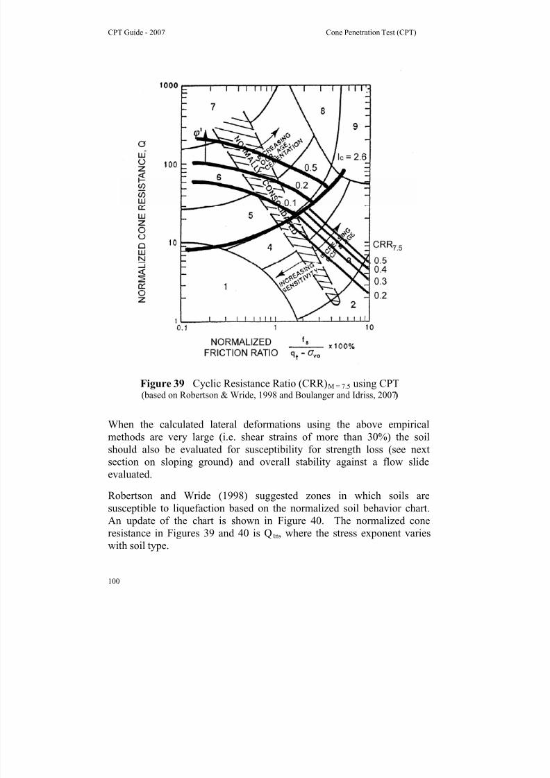
8/13/2019 Cpt Guide Nov 2007 Edition 2
http://slidepdf.com/reader/full/cpt-guide-nov-2007-edition-2 107/126
CPT Guide - 2007 Cone Penetration Test (CPT)
100
Figure 39 Cyclic Resistance Ratio (CRR)M = 7.5 using CPT (based on Robertson & Wride, 1998 and Boulanger and Idriss, 2007)
When the calculated lateral deformations using the above empirical
methods are very large (i.e. shear strains of more than 30%) the soil
should also be evaluated for susceptibility for strength loss (see next
section on sloping ground) and overall stability against a flow slide
evaluated.
Robertson and Wride (1998) suggested zones in which soils are
susceptible to liquefaction based on the normalized soil behavior chart.
An update of the chart is shown in Figure 40. The normalized cone
resistance in Figures 39 and 40 is Qtn, where the stress exponent varies
with soil type.

8/13/2019 Cpt Guide Nov 2007 Edition 2
http://slidepdf.com/reader/full/cpt-guide-nov-2007-edition-2 108/126
CPT Guide - 2007 Cone Penetration Test (CPT)
101
Figure 40 Zones of potential liquefaction based on the CPT
Zone A1 Cyclic liquefaction likely depending on size and duration of
cyclic loading
Zone A2 Cyclic liquefaction and strength loss likely depending on
loading and ground geometryZone B Liquefaction and post-earthquake strength loss unlikely,
check cyclic softening
Zone C Cyclic liquefaction and strength loss possible depending on
soil plasticity, brittleness/sensitivity, strain to peak undrained
strength and ground geometry
8/13/2019 Cpt Guide Nov 2007 Edition 2
http://slidepdf.com/reader/full/cpt-guide-nov-2007-edition-2 109/126
CPT Guide - 2007 Cone Penetration Test (CPT)
102
CPT for Flow Liq uefactio n – Steeply Slop ing Sites
Steeply sloping ground is defined as:
1. Steeply sloping ground (slope angle > 5 degrees)
2. Earth embankments (e.g. dams, tailings structures)
Sequence to evaluate flow liquefaction (i.e. strength loss)
1. Evaluate susceptibility for strength loss
2. Evaluate stability using post-earthquake shear strengths
3. Evaluate if earthquake will trigger strength loss
4. Evaluate deformations.
1. Evaluate Susceptibi l ity For Strength Loss
Use the CPT, plus disturbed samples (for grain size distribution,Atterberg limit and water content) to identify materials that are
susceptible to strength loss due to earthquake shaking, (i.e. loose,
sand-like and sensitive clay-like materials). Use conservative
evaluation techniques, since experience has shown that when
strength loss occurs, instability can be rapid with little warning and
deformations can be very large.
a. Loose, sand-like materials (susceptible to strength loss)
i. Either fines content < 20% or fines content > 35% and
Plasticity Index (PI) < 12 and water content (wc) > 0.85
Liquid Limit (LL)
ii. CPT (q c1N)cs < 70 and SPT (N1)60cs < 14. This represents
the boundary between A1 and A2 in Figure 40.
b. Sensitive Clay-like materials (test for susceptibility, function of
sensitivity and strain to failure)
i. Fines content > 35%, and water content (wc) > 0.85 LL
ii. CPT Zone C (see CPT chart, Figure 40) and/or FVT
(Field Vane Test), where sensitivity, St > 10iii. Strain to failure less than 1%
c. Clay-like materials (not susceptible to strength loss)
i. Fines content > 20% and PI > 12, and water content (wc)
< 0.80 Liquid Limit (LL)
ii. CPT Zone B (see CPT chart, Figure 40)

8/13/2019 Cpt Guide Nov 2007 Edition 2
http://slidepdf.com/reader/full/cpt-guide-nov-2007-edition-2 110/126
CPT Guide - 2007 Cone Penetration Test (CPT)
103
If layers/zones of low permeability exist that could inhibit pore water
redistribution after seismic loading and promote void redistribution,
increase conservatism when evaluating susceptibility for strength loss.
2. Evaluate Stabil ity Using Post-earthquake Shear Strengths
a. Initial stability analysis assuming strength loss is triggered and
using conservative estimates of minimum (liquefied
/residual/steady state) undrained shear strength, Sur , based on
either empirical correlations with in-situ tests or field measured
values:
i. sur /σ'vc or sur from CPT in loose sand-like materials (either
Olson and Stark, 2002 or Idriss and Boulanger, 2007)
Assume sur /σ'vc ~ 0.05, if no data available.ii. Use remolded undrained shear strength, sur , for sensitive
clay-like materials measured from either CPT or FVT
iii. 80% of peak undrained shear strength, sup, measured
using either CPT or FVT in clay-like materials
iv. In zones where strength loss does not occur, use peak
undrained shear strength, sup (or drained strength,
whichever is lower)
If Factor of Safety (FS) > 1.2, assume stability is acceptableand check deformations
If FS < 1.2, evaluate material behavior and triggering in more
detail
• For low risk structures, redesign or modify
• For moderate and high risk structures, carry out more
detailed investigation
b. If project risk is moderate to high risk and FS < 1.2, evaluate
post-earthquake shear strength in more detail:i. Additional in-situ testing, e.g. SCPT, FVT, geophysical
logging.
ii. High quality undisturbed samples and appropriate
laboratory testing.

8/13/2019 Cpt Guide Nov 2007 Edition 2
http://slidepdf.com/reader/full/cpt-guide-nov-2007-edition-2 111/126
CPT Guide - 2007 Cone Penetration Test (CPT)
104
• If FS > 1.2, assume stability is acceptable and check
deformations
• If FS < 1.2, check triggering
If layers/zones of low permeability exist that could inhibit pore
water redistribution after seismic loading and promote void
redistribution, increase conservatism when evaluating post
earthquake shear strengths. For high risk projects, the potential for
void redistribution can be evaluated using complex effective stress
numerical models.
3. Evaluate I f Earthquake Wil l Tr igger Strength Loss
When FS < 1.0 using best estimates of post-earthquake shearstrength parameters, assume that strength loss will be triggered.
When 1.0 < FS < 1.2 using best estimates of post-earthquake shear
strength parameters, check if the earthquake will trigger strength
loss by applying either of the following approaches:
a. Pore-pressure approach, using CRR (Youd et al. 2001)
b. Strain-based approach (Castro, 1999)
c. Yield-strength approach (Sladen , 1985, Olsen and Stark, 2003)
All approaches should be based on improved knowledge of
materials based on combined results from in-situ tests and
appropriate laboratory testing on high quality samples. When soils
are susceptible to strength loss and slopes are steep, a trigger
mechanism should always be assumed to be present (Silvis and de
Groot, 1995). Hence, for high risk structures caution and
conservatism should be exercised.
If one or more zones are not expected to trigger strength loss, re-evaluate stability using higher shear strength in these zones.
• If FS > 1.2, assume stability is acceptable and check
deformations.
• If FS < 1.2 assume unsafe and redesign or modify.
8/13/2019 Cpt Guide Nov 2007 Edition 2
http://slidepdf.com/reader/full/cpt-guide-nov-2007-edition-2 112/126
CPT Guide - 2007 Cone Penetration Test (CPT)
105
4. Evaluate Seismic Deformations
If embankment is considered stable, evaluate seismic deformations
based on size and duration of earthquake shaking.
a. Preliminary screening
i. If no initial liquefaction is identified and earthquake is
small, assume deformations are small.
b. Pseudo-static analysis
i. If earthquake is small, M < 7, and,
ii. If no significant zones indicate cyclic liquefaction, and,
iii. Small deformations (less than 3 feet) are not significant to
the performance of the embankment
Use limit equilibrium stability analyses using pseudo-static
seismic coefficient of 0.5 PGA and 80% of peak undrainedstrength for clay-like and sand-like materials (but not to
exceed 80% of drained strength).
• If 1.0 < FS < 1.2, deformations are likely to be less than
1m (3 feet).
c. Newmark-type analyses (no seismic liquefaction/cyclic
mobility)
Perform a Newmark-type analysis if no zones of materialindicate cyclic liquefaction.
d. Numerical modeling (cyclic liquefaction)
Perform appropriate numerical analyses (finite
element/finite difference) that incorporate special
provisions for pore pressure build-up.

8/13/2019 Cpt Guide Nov 2007 Edition 2
http://slidepdf.com/reader/full/cpt-guide-nov-2007-edition-2 113/126
CPT Guide - 2007 Cone Penetration Test (CPT)
106
Ground Improvement Compaction Control
Ground improvement can occur in many forms depending on soil type
and project requirements. For non-cohesive soil such as sands, silty sands
and so on, deep compaction is a common ground improvement technique.
Deep compaction can comprise: vibrocompaction, vibroreplacement,
dynamic compaction, compaction piles, and deep blasting.
The CPT has been found to be one of the best methods to monitor and
document the effect of deep compaction due to the continuous, reliable
and repeatable nature of the data. Most deep compaction techniques
involve cyclic shear stresses in the form of vibration to induce an increase
in soil density. Vibratory compaction is generally more effective in soil
deposits with a friction ratio less than 1%. When the friction ratio
exceeds about 1.5% vibratory compaction is usually not effective. Theserecommendations apply to average values in a soil deposit. Local seams
or thin layers with higher friction ratio values are often of little practical
importance for the overall performance of a project and their effect should
be carefully evaluated when compaction specifications are prepared. The
zone of soil behavior where vibratory compaction is most applicable is
shown on the CPT soil behavior charts in Figure 41. Soils with an initial
cone resistance below about 3 MPa (30 tsf) can be compressible or
contain organic matter, silt or clay and will not respond well to vibratory
compaction. Soils with a high initial cone resistance will not show
significant compaction and generally do not need compaction. It is also
important to establish the level and variation of the groundwater table
before compaction since some compaction methods are less effective in
dry or partially saturated soils. The CPTU provides the required
information on groundwater conditions.
Often the aim of deep compaction is for one or more of the following:
• increase bearing capacity (i.e. increase shear strength)
• reduce settlements (i.e. increase stiffness)• increase resistance to liquefaction (i.e. increase density).
The need for deep compaction and geotechnical conditions will be project
specific and it is important that design specifications take account of these
site specific requirements. Cone resistance in cohesionless soils is
governed by many factors including soil density, in-situ stresses, stress

8/13/2019 Cpt Guide Nov 2007 Edition 2
http://slidepdf.com/reader/full/cpt-guide-nov-2007-edition-2 114/126
CPT Guide - 2007 Cone Penetration Test (CPT)
107
history, and soil compressibility. Changes in shear strength, stiffness and
density can be documented with changes in measured cone resistance.
A common problem in many deep compaction projects is to specify a
minimum value of q c for compaction over a large depth range. This
results in a variation of relative density with depth, with the required
degree of compaction near the surface being much higher than at depth.
For certain projects, a high degree of compaction close to the ground
surface may be justified.
Figure 41 Guidelines for soils suitable for vibrocompaction techniques.
However, this can be very difficult to obtain with certain deep compaction
techniques and this decision should be based on engineering judgment
related to the geotechnical project requirements. It is generally preferred

8/13/2019 Cpt Guide Nov 2007 Edition 2
http://slidepdf.com/reader/full/cpt-guide-nov-2007-edition-2 115/126
CPT Guide - 2007 Cone Penetration Test (CPT)
108
to specify a minimum normalized value of cone resistance corrected for
overburden stress, Qtn. Since, grain characteristics can vary rapidly in
many sandy deposits, it is preferred to specify an acceptance criteria based
on normalized clean sand equivalent values of cone resistance,(q c1N)cs (or (Q
tn)
cs), using the methodology shown in Figure 37, especially when
compaction is performed to reduce the potential for liquefaction.
Specification using (q c1N)cs can reduce problems in silty zones, where
traditional approaches have often resulted in excessive ground
improvement in an effort to reach unrealistic criteria.
An important aspect of deep compaction which is not yet fully understood
is the increase in cone resistance with time after compaction. This time
effect has been observed in different ground conditions and with different
compaction methods. Often no measurable change in pore pressure has
been observed and the increase takes place without visible groundsettlements. Charlie et al. (1992) studied a number of cases where cone
resistance was measured with time after compaction. A range of
compaction techniques were used and the results are shown in Figure 42.
The cases were representative of a wide range of climates and geologic
conditions with average temperatures varying from -10oC (Beaufort Sea)
to +27oC (Nigeria). Charlie et al. (1992) suggested that the time effect
could be linked to the average air temperature. The possibility of time
effects should be evaluated for each project. For very large projects, it
may be necessary to perform field trials.
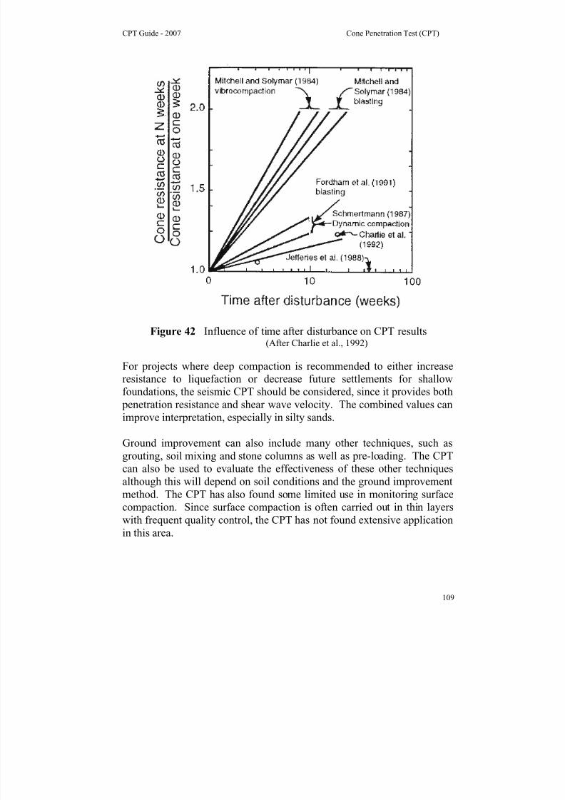
8/13/2019 Cpt Guide Nov 2007 Edition 2
http://slidepdf.com/reader/full/cpt-guide-nov-2007-edition-2 116/126
CPT Guide - 2007 Cone Penetration Test (CPT)
109
Figure 42 Influence of time after disturbance on CPT results(After Charlie et al., 1992)
For projects where deep compaction is recommended to either increaseresistance to liquefaction or decrease future settlements for shallow
foundations, the seismic CPT should be considered, since it provides both
penetration resistance and shear wave velocity. The combined values can
improve interpretation, especially in silty sands.
Ground improvement can also include many other techniques, such as
grouting, soil mixing and stone columns as well as pre-loading. The CPT
can also be used to evaluate the effectiveness of these other techniques
although this will depend on soil conditions and the ground improvementmethod. The CPT has also found some limited use in monitoring surface
compaction. Since surface compaction is often carried out in thin layers
with frequent quality control, the CPT has not found extensive application
in this area.
8/13/2019 Cpt Guide Nov 2007 Edition 2
http://slidepdf.com/reader/full/cpt-guide-nov-2007-edition-2 117/126
CPT Guide - 2007 Cone Penetration Test (CPT)
110
Design of Wick or Sand Drains
Pre-loading is a common form of ground improvement in fine grained
soils where the rate of consolidation is important. Installation of sanddrains or wick drains can significantly decrease the time for consolidation
settlements. Prior to 1975, vertical sand drains were common to aid
consolidation with temporary pre-load. Since 1975, geosynthetics in the
form of wick drains have dominated the market. Wick drains are usually
fluted or corrugated plastic or cardboard cores within geotextile sheaths
that completely encircle those cores. They are usually 100 mm wide by 2
to 6 mm thick. The wick drain is usually pushed or driven into the ground
to the desired depth using a lance or mandrel. The drain then remains in
place when the lance or mandrel is removed. Installation can be in therange of 1 to 5 minutes depending on ground conditions, pushing
equipment and depth of installation. The design of wick drains is not
standardized but most equate the diameter of the particular type of drain
to an equivalent sand drain diameter.
The method developed by Hansbo (1970) is commonly used, and the
relevant design equations are as follows:
[ ] U1
1
n175.0)d /Dln(c8
D
th
2
−−=
Where: t = consolidation
ch = coefficient of consolidation for horizontal flow
d = equivalent diameter of the wick drain
( −~ circumference/π)
D = sphere of influence of the wick drain (for a triangular
pattern use 1.05 times the spacing, for a square pattern use 1.13
times the spacing).
U = average degree of consolidation
The key input parameter for the soil is the coefficient of consolidation for
horizontal flow, ch. This parameter can be estimated from dissipation
tests using the CPTU. The value derived from the CPTU is particularly
useful since, the cone represents a very similar model to the installation
8/13/2019 Cpt Guide Nov 2007 Edition 2
http://slidepdf.com/reader/full/cpt-guide-nov-2007-edition-2 118/126
CPT Guide - 2007 Cone Penetration Test (CPT)
111
and drainage process around the wick drain. Although there is some
possible smearing and disturbance to the soil around the CPT, similar
smearing and disturbance often exists around the wick, and hence, the
calculated value of ch from the CPTU is usually representative of the soil
for wick drain design.
Details on estimation of ch from dissipation tests were given in the section
on (geotechnical parameters) consolidation characteristics. To provide a
reasonable estimate of ch a sufficient number of dissipation tests should be
carried out through the zone of interest. The dissipation tests should be
carried out to at least 50% dissipation. Several dissipation tests should be
carried out to full dissipation to provide an estimate of the equilibrium
groundwater conditions prior to pre-loading.
8/13/2019 Cpt Guide Nov 2007 Edition 2
http://slidepdf.com/reader/full/cpt-guide-nov-2007-edition-2 119/126
CPT Guide - 2007 Main References
112
Main References
Lunne, T., Robertson, P.K., and Powell, J.J.M 1997. Cone penetration
testing in geotechnical practice, E & FN Spon Routledge, 352 p, ISBN0-7514-0393-8.
Jefferies, M.G. and Davies, M.P. 1993. Estimation of SPT N values from
the CPT, ASTM.
Robertson, P.K. 1990. Soil classification using the cone penetration test.
Canadian Geotechnical Journal, 27 (1), 151-8.
Robertson, P.K., Campanella, R.G. and Wightman, A. 1983. SPT-CPT
Correlations, ASCE J. of Geotechnical Engineering 109(11): 1449-59.
Baligh, M.M. and Levadoux, J.N. 1986. Consolidation after undrained
piezocone penetration, II: Interpretation, J. of Geotech. Engineering,
ASCE, 112(7): 727-745.
Jamiolkowski, M., Ladd, C.C., Germaine, J.T. and Lancellotta, R. 1985.
New developments in field and laboratory testing of soils, State-of-
the-art report, Proceedings of the 11th
International Conference on
Soil Mechanics and Foundation Engineering, San Francisco, 1, 57-153, Balkema.
Robertson, P.K., Sully, J.P., Woeller, D.J., Lunne, T., Powell, J.J.M. and
Gillespie, D.G. 1992. Estimating coefficient of consolidation from
piezocone tests, Canadian Geotechnical J., 29(4): 551-557.
Teh, C.I. and Houlsby, G.T. 1991. An analytical study of the cone
penetration test in clay, Geotechnique, 41(1): 17-34.
Robertson, P.K. and Wride, C.E., 1998. Cyclic Liquefaction and its
Evaluation based on the CPT Canadian Geotechnical Journal, 1998,
Vol. 35, August.

8/13/2019 Cpt Guide Nov 2007 Edition 2
http://slidepdf.com/reader/full/cpt-guide-nov-2007-edition-2 120/126
CPT Guide 2007 Main References
113
Youd, T.L., Idriss, I.M., Andrus, R.D., Arango, I., Castro, G.,
Christian, J.T., Dobry, R., Finn, W.D.L., Harder, L.F., Hynes, M.E.,
Ishihara, K., Koester, J., Liao, S., Marcuson III, W.F., Martin, G.R.,
Mitchell, J.K., Moriwaki, Y., Power, M.S., Robertson, P.K., Seed, R.,
and Stokoe, K.H., Liquefaction Resistance of Soils: Summary Report
from the 1996 NCEER and 1998 NCEER/NSF Workshop on
Evaluation of Liquefaction Resistance of Soils, ASCE, Journal of
Geotechnical & Geoenvironmental Engineering, Vol. 127, October, pp
817-833
Zhang, G., Robertson. P.K., Brachman, R., 2002, Estimating
Liquefaction Induced Ground Settlements from the CPT, Canadian
Geotechnical Journal, 39: pp 1168-1180
Zhang, G., Robertson. P.K., Brachman, R., 2004, EstimatingLiquefaction Induced Lateral Displacements using the SPT and CPT,
ASCE, Journal of Geotechnical & Geoenvironmental Engineering,
Vol. 130, No. 8, 861-871

8/13/2019 Cpt Guide Nov 2007 Edition 2
http://slidepdf.com/reader/full/cpt-guide-nov-2007-edition-2 121/126
GEOTECHNICAL SERVICES
Q U A L I T Y • S A F E T Y • V A L U E
Geotechnical Capabilities:
▪ Cone Penetrat ion Testing (CPT)
▪ Seismic Cone Penetration Testing
▪ Mud Rotary and Hollow Stem Auger Drilling
▪ Soil and Rock Coring
▪ SPT Energy Calibration
▪ Diamond Coring
▪ Soil Coring
▪ Vane Shear Test
▪ Pressuremeter Testing
▪ Dilatometer Testing
▪ Vibra Core Sampling
Quality isn’t someth ing we test for after the job is done. It’s a way of doing business,
an integral part of our daily activities that we instill in our personnel, something we build into our
technologies, a guarantee of value that we deliver with all our services.
Gregg Drilling & Testing, Inc. (Gregg) offers a wide range of services for environmental,
geotechnical, and marine site investigation. The Gregg professionals have the training and experienceto fully understand the needs of each client, identify the unique job requirements, and provide the
highest quality services.

8/13/2019 Cpt Guide Nov 2007 Edition 2
http://slidepdf.com/reader/full/cpt-guide-nov-2007-edition-2 122/126
ENVIRONMENTAL SERVICES
Environmental Capabilities:
▪ Well Installation, Development & Abandonment
▪ Groundwater Extraction & Monitoring Wells
▪ Vapor Extraction, Sparge & Bio Vent Wells
▪ Nest Wells, Cluster Wells, Multipoint Sampling Systems
▪ Cone Penet ration Testing with UVIF & Resistivity
▪ Hollow Stem Auger & Mud Rotary Drilling
▪ Direct Push Soil, Groundwater & Vapor Sampling
▪ Air Vacuum Excavation
▪ Well Rehabilitation (submersible & turbine)
▪ Pump Installation & Repair
▪ Video Logging
▪ Hydraulic Fracturing
Protecting our workforce, our clients, and the general public from injuries and hazardous
incidents that may be harmful and disruptive is a core element of our corporate culture. Because
of this we have dedicated ourselves to a “safety first” philosophy which applies to all areas ofoperation and is put into practice by all Gregg personnel on a daily basis. This philosophy has
allowed us to effectively manage the risks inherent in our industry and consistently provide a safe,
sensible, and productive work environment.
Q U A L I T Y • S A F E T Y • V A L U E

8/13/2019 Cpt Guide Nov 2007 Edition 2
http://slidepdf.com/reader/full/cpt-guide-nov-2007-edition-2 123/126
MARINE SERVICES
Marine Capabilities:
▪ Mud Rotary Drilling
▪ Cone Penetrat ion Testing (CPT)
▪ Mini-Cone Penetration Testing
▪ Seismic CPT
▪ Downhole Vane Shear Testing (VST)
▪ Micropile Installation
▪ Vibra Core Sampling
▪ Piston Sampling
▪ Gravity Coring
Testing Equipment:
▪ Mobile B-80/22 and B80/14 Mud Rotary Drill Rig
▪ Miniature CPT System (2 cm2 cone) - depths of up to 5000 feet
▪ CPT Portable System (10 cm2 & 15 cm2 cone, drill rig deployed)
▪ Vibracore Sampling System - up to 20 feet of core
▪ Gravity Core Sampling System - up to 5 feet of core
Platforms Offered:
▪ Quin Delta Drill Ship ▪ Tugboats
▪ Jack-up Boats & Barges ▪ Support Vessels▪ Sectional Barges
Q U A L I T Y • S A F E T Y • V A L U E

8/13/2019 Cpt Guide Nov 2007 Edition 2
http://slidepdf.com/reader/full/cpt-guide-nov-2007-edition-2 124/126
Gregg acquires geotechnical and environmental data using a variety of unique in-house
equipment, tools, sensors, and techniques ranging from cone penetration testing and geophysical methods
to conventional drilling procedures and borehole tests. In addition we offer an array of highly specialized
services including:
▪ CPT with UVIF & Resistivity
▪ Seismic CPT
▪ SPT Energy Calibration
▪ Vane Shear Testing
▪ Pressuremeter Testing
▪ Dilatometer Testing - Flat & Rock
▪ Settlement Monitoring
▪ Goodman Jack Testing
▪ CPT Data Cross Sections
Our advanced data collection techniques, equipment, and monitoring systems combined with
the expertise of our personnel enables us to provide exceptional performance and value time after time.
SPECIALIZED SERVICES
Q U A L I T Y • S A F E T Y • V A L U E

8/13/2019 Cpt Guide Nov 2007 Edition 2
http://slidepdf.com/reader/full/cpt-guide-nov-2007-edition-2 125/126
10 Feet
6 Feet
COMMUNICATION
CATV

8/13/2019 Cpt Guide Nov 2007 Edition 2
http://slidepdf.com/reader/full/cpt-guide-nov-2007-edition-2 126/126
GREGG DRILLING & TESTING, INC.
CORPORATE HEADQUARTERS
2726 WALNUT AVENUE; SIGNAL HILL, CALIFORNIA 90755
Tel: (562) 427-6899 Fax: (562) 427-3314
www.greggdrilling.com
SOUTHERN CALIFORNIA
Signal Hill, California
(Corporate Headquarters)
(562) 427-6899
•SOUTHERN CALIFORNIA
•NORTHERN CALIFORNIA
SOUTHWEST
•