Why Bode? The great popularity of Bode magnitude plots stems from the following useful properties of logarithms:

If kl

mn

dscsbsassH

)()()()()(

++++

= then

[ ] )(log)(log)(log)(log)(log 1010101010 dskcslbsmasnsH +−+−+++=

Thus the magnitude functions are asymptotic to straight lines on a log-log plot. dB or not dB? That is the question Bode Plots are Magnitude and Phase versus frequency graphs. There are two log-log conventions for plotting magnitude versus frequency: log magnitude and decibels (dB). Decibels (dB) to Magnitude Conversion Magnitude dB = 20log10(Magnitude) Magnitude Conversion to Decibels (dB) Magnitude = 10(Magnitude dB)/20 Here is a conversion table:

Decibel ExamplesMagnitude dB1,000,000,000 +180100,000,000 +16010,000,000 +1401,000,000 +120100,000 +10010,000 +801,000 +60100 +4010 +204 +2 +1 01/2 -61/4 -12

0.1 -200.01 -400.001 -600.0001 -800.00001 -1000.000001 -1200.0000001 -1400.00000001 -1600.000000001 -180

126

Bode Plot Slopes for Poles and Zeros at the Origin

Bode Plot with Magnitude on a dB Scale in MATLAB % Magnitude of a Transfer Function on a dB Plot % Save output figures in bitmap mode for best quality s = tf('s'); H = 0.010*(s + 20)/((s + 1)*(s + 7000)); [mag phase w] = bode(H); %Magnitude in dB not on log scale mag2 = 20*log10(mag); figure; semilogx(w, reshape(mag2, 1, length(mag2)), 'LineWidth', 2); grid minor; %finer grid xlabel('\omega (rad/s)'); ylabel('Magnitude in dB'); figure; semilogx(w, reshape(phase, 1, length(phase)), 'LineWidth', 2); grid minor; %finer grid xlabel('\omega (rad/s)'); ylabel('Phase (degrees)'); ______________________________________________________________________

Bode Plot with Magnitude on Log Scale in MATLAB %Log Magnitude Plot % Save output figures in bitmap mode for best quality s = tf('s'); H = (s + 50)/((s + 10)*(s + 60000)); [mag phase w] = bode(H); figure; loglog(w, reshape(mag, 1, length(mag)), 'LineWidth', 2); grid on; xlabel('\omega (rad/s)'); ylabel('Magnitude'); figure; semilogx(w, reshape(phase, 1, length(phase)), 'LineWidth', 2); grid on; xlabel('\omega (rad/s)'); ylabel('Phase (degrees)');

Stability from Bode PlotsL(jω)

Closed Loop System is stable provided the Gain of L(jω) is less than 1 AND the phase of L(jω) is less than 180o for all ω

Let ωπ be the phase cross over frequency where the phase of the open loop transfer function crosses 180o

Let ωg be the gain cross over frequency where the open loop gain crosses 1.

Gain Margin = 1/|L(jωπ )| and Phase Margin = arg L(jωg)+π

System is marginally stable when Gain Margin = 0 dB AND Phase Margin = 0o (i.e., ωg = ωπ )

Gain & Phase Margin Defined

arg L(jω)

ωg

ωg

ω

ωωπ

ωπ

|L(jω)|

O

O

-180o

1

Gain Margin

Phase Margin=arg L(jωg)+π

1= |L(jωπ )|

FINDING CLOSED LOOP STABILITY MARGINS FROM THE OPEN LOOP GAIN

Problem: For the Open Loop Magnitude and Phase Plots shown below, find 1) Gain Crossover Frequency, ωg 2) the Phase Crossover Frequency, ωπ 3) Gain Margin (linear and dB), and 4) the Phase margin (in degrees and radians)

|L(jω

)|

dB 135.422.01

)(1

: MarginGain

=≈==gjL

Kω

ωπωg

L(jω)K-

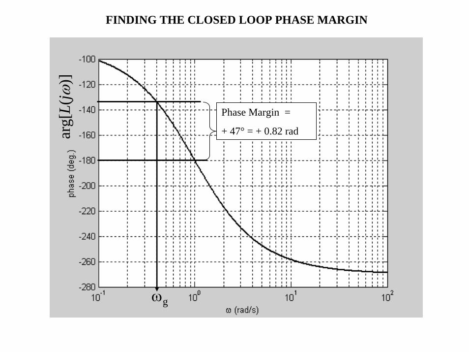
FINDING THE CLOSED LOOP PHASE MARGIN

Phase Margin =

+ 47° = + 0.82 radarg[

L(jω

)]

ωg

EXAMPLE: FINDING K FOR A GIVEN PHASE MARGIN REQUIREMENTProblem: Find the value of K such that the open loop system with the frequency response shown has a closed loop PM of +20° (and thus the closed loop system is stable). (When PM=0°, K is Gain Margin)

22.245.01

)(1

===djL

Kω

L(jω)K-

|L(jω

)|

EXAMPLE: FINDING K FOR A GIVEN PHASE MARGIN REQUIREMENT

PM = + 20°

.sec/7.0 radd =ω

arg[

L(jω

)]

CHAPTER 6 FREQUENCY RESPONSEMAGNITUDE PLOT FOR K=2.22

|KL(

jω)|

.sec/7.0 radd =ω

CHAPTER 6 FREQUENCY RESPONSEPHASE PLOT FOR K=2.22

PM = + 20°

arg[

KL(

jω)]

What is the open loop transfer function KL(jω) for the system whose magnitude and phase plots are shown on the previous few slides?

21

1)(

⎟⎠⎞⎜

⎝⎛ +

=

o

jj

KjKL

ωωω

ω

Inspection of magnitude and phase plot indicates that KL(jω) is of the form:

where |KL(jω)|ω=0.10 =10 ≈ |K1/(jω)|ω=0.10 = K1/ω ω=0.10 = 10K1 => K1 =1

φ(ω=ωo) = φ[1/(jωo)] + φ{1/[1+j(ωo/ωo)]2} = -90o-90o= -180o =>ωo = 1

Hence the transfer function is:

( )211)(

ωωω

jjjKL

+=

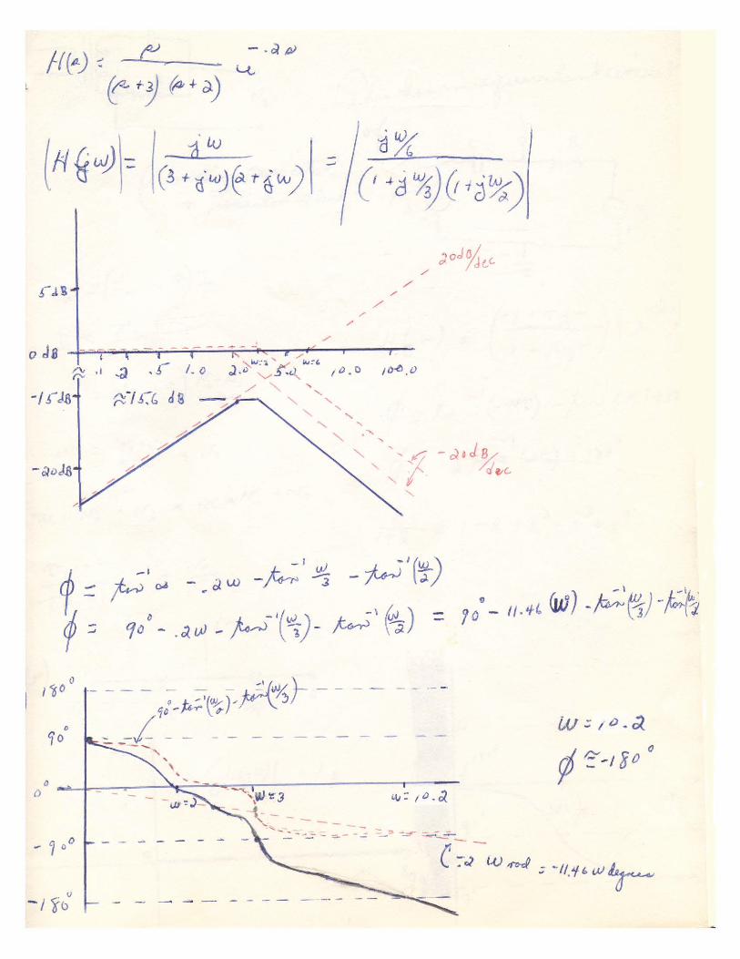
MATLAB CODE: >> sys =tf([1 0],[1 5 6]) Transfer function: s ------------- s^2 + 5 s + 6 >> sys.outputd=0.2 Transfer function: s exp(-0.2*s) * ------------- s^2 + 5 s + 6 >> margin(sys)

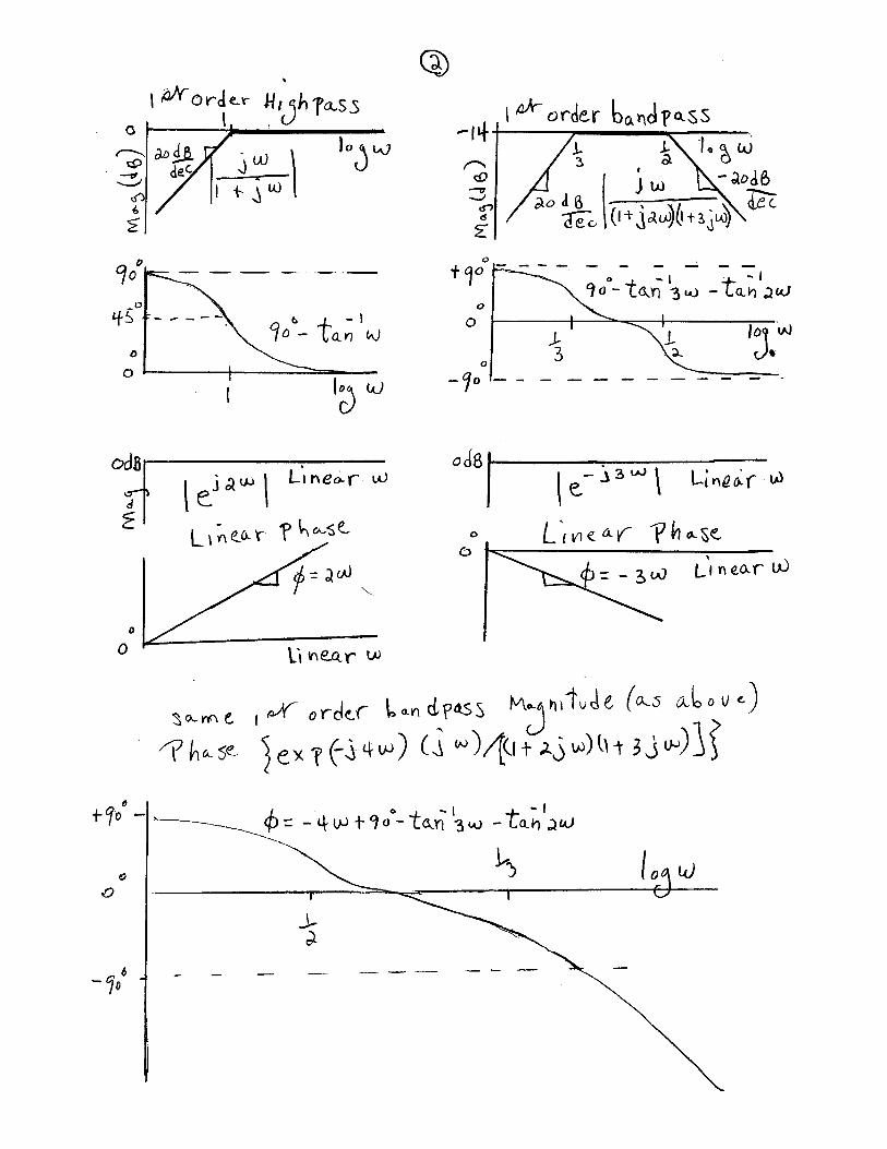
Derive the Magnitude and Phase of the following functions of ω and plot both the Magnitude and Phase functions on the ω axis using the same logarithmic scale for 0< ω <∞. These are often referred to as Bode plots. a) jω b) (jω)2 c) (jω)3 d) 1/jω e)1/(jω)2 d)1/(jω)3

c) 1+jω d) (1+jω)2 e) 1/(1+jω) f) 1/(1+jω)2 g) (1+j3ω)/(1+j2ω) h) (1+j2ω)/(1+j3ω) i) jω/(1+jω) j) jω/[(1+j2ω)(1+j3ω)] l) exp(j2ω) m) exp(-j3ω) n) exp(-j4ω)jω/[(1+j2ω)(1+j3ω)] o) X(jω) = 2sin(ωT)/ ω

π /T

π

0−π /T

X(jω) = 2sin(ωT)/ω

φ(ω) = 2sin(ωT)/ω

ω

Magnitude

Phase