cpaa design manual · pressure pipelines 57 ... hydraulics of precast concrete conduits 3 preface t...

CPAA DESIGN MANUAL

Concrete Pipe Associationof Australasia


Hydraulics of PrecastConcrete Conduits

PIPES AND BOX CULVERTS

1



Hydraulics of PrecastConcrete ConduitsPIPES AND BOX CULVERTS

CPAA DESIGN MANUAL

Hydraulics of PrecastConcrete Conduits

PIPES AND BOX CULVERTS

HYDRAULICS OF PRECAST CONCRETE CONDUITS

2

Contents

PREFACE 3

NOTATIONS AND SYMBOLS 4

SECTION 1FLOW OF WATER IN PRECAST CONCRETE CONDUITS 5

SECTION 2STORMWATER RUNOFF 17

SECTION 3CULVERTS 27

SECTION 4STORMWATER DRAINAGE SYSTEMS 41

SECTION 5SEPARATE SEWERAGE SYSTEMS 51

SECTION 6PRESSURE PIPELINES 57

First published 1983, reprinted 1986, 1991, 2007 and 2012 with minor modifications.


3

Preface

This manual has been prepared to assist engineers with the hydraulic design of precast

concrete conduits. It is hoped it will also be useful in the field of engineering education.

It consolidates information from several sources and presents it in a practical and usable form.

The first section is a precise treatment of theoretical hydraulic concepts used in the manual.

It should be used when necessary to assist with the understanding of the subsequent

subjects. The remaining five sections consider the practical design aspects of individual

subjects, namely, runoff, culverts, drains, sewers and pressure pipes. Each of the latter

sections concludes with worked examples which may be used as models for many practical

problems. If more detailed information is required, references are listed at the end of each

section.

The Concrete Pipe Association of Australasia is indebted to many individual and institutional

researchers and scientists for the information given.

The Concrete Pipe Association of Australasia believes that the information given in this

manual is the most up-to-date and correct available within each subject, but beyond this

statement no guarantee is given nor is any responsibility assumed by the Association and its

members.

Comments and suggestions for improvements to the manual will be welcomed and should

be directed to the Association at [email protected].

Concrete Pipe Association of Australasia

January 2012


4

Notations and Symbols

A Cross sectional area of conduit, or catchment areaC Hazen Williams coefficient or coefficient of runoffD Pipe diameterE Modulus of elasticityF A coefficientFp Passive soil resistanceH Energy head or height of thrust blockHb Bend head lossHc Contraction or expansion head lossHe Entry head lossHf Uniform head lossHo Outlet head lossHs Specific energyHv Valve head lossHW HeadwaterI Rainfall intensity or infiltration allowanceK Bulk modulus of compression for waterL Length of conduitP Wetted perimeterQ DischargeR Hydraulic RadiusRe Reynolds number, D/T ThrustTW Tailwater

a Pressure wave velocity or speedc Soil cohesiond Peak factordc Critical depthe Thickness of pipe wallf Resistance factorg Acceleration due to gravityh A heightk Roughness factorkb Bend loss coefficientkc Contraction or expansion loss coefficientke Entry head loss coefficientko Outlet head loss coefficientkv Valve head loss coefficientn Manning’s or Kutter’s np Hydraulic pressures Tangent to slope of the energy linesc Tangent to critical slopeso Tangent to slope of culvert invertt Critical time or time of concentrationv Flow velocityy Depth of flowz Conduit elevation above base level

An angle Unit weight of waters Unit weight of soil An angle Kinematic viscosity of water Density of water Boundary shear

[ ] Brackets surrounding reference number listed at end of section

FLOW OF WATER IN PRECAST CONCRETE CONDUITS SECTION 1

5

SECTION 1

1. FLOW OF WATER IN PRECAST CONCRETE CONDUITS

1.1 PHYSICAL PROPERTIES OF WATER

1.2 FULL FLOW 1.2.1 THE ENERGY LINE 1.2.2 ENERGY LOSSES AT CROSS SECTIONAL CHANGES 1.2.3 ENERGY LOSS AT UNIFORM FLOW 1.2.3.1 GENERAL

1.2.3.2 THE COLEBROOK–WHITE EQUATION

1.2.3.3 MANNING'S FORMULA

1.2.3.4 HAZEN WILLIAMS' FORMULA

1.2.3.5 SELECTION OF APPROPRIATE VALUES

1.3 PART-FULL FLOW 1.3.1 UNIFORM FLOW 1.3.1.1 ENERGY LOSSES AT SECTIONAL CHANGES

1.3.1.2 UNIFORM ENERGY LOSSES

1.3.1.3 FLOWING VELOCITY IN CLOSED CONDUITS

1.3.2 NON-UNIFORM FLOW 1.3.2.1 GENERAL

1.3.2.2 CRITICAL DEPTH

1.3.2.3 CRITICAL SLOPE

1.3.2.4 THE HYDRAULIC JUMP

1.4 BOUNDARY SHEAR

1.5 WATER HAMMER 1.5.1 THE NATURE OF WATER HAMMER 1.5.2 VALVE CLOSURE 1.5.3 PUMP STOPPAGE 1.5.4 WAVE SPEED

1.6 REFERENCES

HYDRAULICS OF PRECAST CONCRETE CONDUITSSECTION 1

6

1.1 PHYSICAL PROPERTIES OF WATER

Various physical properties of water are of impor-tance in hydraulic calculations. These properties are set out in Table 1.1.

Table 1.1 PHYSICAL PROPERTIES OF WATER [1.1]

1.2 FULL FLOW

1.2.1 THE ENERGY LINE

The concept of the energy line representing the height above a base level of the sum:

z + p/ + v2/2g

is used generally for all full-flowing conduits. It repre-sents the energy in a weight unit of water when passing a given section.

Figure 1.1

From Figure 1.1 follows:

z1 + p1/ + v2/2g = z2 + p2/ + v2/2g + Hf or Hf = (z1 – z2) + (p1/ − p2/ ) where Hf is the energy loss over the length L is the unit weight of water and p the hydraulic pressure p/ is referred to as the hydraulic head and v2/2g as velocity head.

The expression is general and applies whether the conduit is rising, falling or horizontal. If the conduit cannot sustain pressure we have:

Hf = z1 − z2

and only downhill flow is possible.

1.2.2 ENERGY LOSSES AT CROSS SECTIONAL CHANGES

Figure 1.2

The energy line around a standpipe (manhole) with a cross section significant in comparison to the conduit cross section is shown on Figure 1.2.

Note a drop He, where the flow enters the standpipe and a drop Ho, where it leaves.

These energy losses are caused by local turbulence resulting from the changes in cross section. It is cus-tomary to express these losses in terms of the velocity head in the conduit.

Entry loss, He = ke v2/2g

Outlet loss, Ho = ko v2/2g

The loss coefficients ke and ko depend on the geometry of the inlet and outlet respectively. Usually they range between 0 and 1 but can be higher for pits with lateral flow entering. A similar approach is adopted to the head losses caused by other fixtures in a pipeline such as bends and valves [1.2] and par-ticular attention is drawn to outlets into large res-ervoirs where the whole velocity energy is lost. (See Figure 1.3.) Loss coefficients for various fittings are set out in Table 1.2.

Figure 1.3

1. FLOW OF WATER IN PRECAST CONCRETE CONDUITS

Temp Specific Kinematic Bulk Modulus of Vapour C˚ Mass Viscosity Compression Pressure

kg/m3 m2/s N/mm2 N/mm2

0 1000 1.79 x 10–6 2000 0.6 x 10–3

10 1000 1.31 x 10–6 2070 1.2 x 10–3

20 998 1.01 x 10–6 2200 2.3 x 10–3

30 996 0.81 x 10–6 2240 4.3 x 10–3

Table 1.2 ENERGY LOSS COEFFICIENTS FOR PIPE FITTINGS [1.1]


7

1.2.3 ENERGY LOSS AT UNIFORM FLOW

1.2.3.1 GENERAL

An expression for the energy loss in pipes was first proposed by Darcy in 1857 by modifying Chezy’s equation designed for open channels and published in 1775.

Darcy’s equation is written: L v2

Hf = f D 2g

where D is the pipe diameter. It is noted that the energy loss is related to the velocity head as are losses due to sectional changes dealt with in Section 1.2.2. The difficulty in applying Darcy’s equation is that the resistance factor, f, is not constant, but varies with conduit roughness as well as v and D.

Numerous equations have been proposed over the years following tests with various pipe materials and mostly within narrow ranges of v and D. These equa-tions are usually of an exponential form and, as later work has shown, are only valid within limited ranges of diameter and flow velocity.

*Charts are located at the back of this manual.

1.2.3.2 THE COLEBROOK–WHITE EQUATION

The Equation now favoured by most is that of Colebrook– White, first proposed in 1939. Unlike the exponential equations it is soundly based physically, but until the advent of computers in engineering design its complex form has made design engineers reluctant to use it.

The equation is written:

1 = –2log10

( k + 2.51 ) f 3.7D Ref

k is roughness coefficientRe Reynolds number vD/ Kinematic viscosity of water (m2/s) (see Table 1.1)

Flow charts based on this equation are graphed in Figures 1.8 to 1.11 for k = 0.06 to 1.5.* The recom-mended k−values are given in the following sections dealing with special conduit applications.

The Colebrook–White equation applies to what is termed 'Transition flow', i.e. the flow pattern which occurs when the flow changes from 'Smooth turbulence' to 'Rough Turbulence'. This is illustrated in Figure 1.4 which shows f as a function of Re with k/D as a para-meter calculated from the Colebrook–White equation.

Bends Hb = kb v2/2g Value of r/D

Bend angle Sharp 1 2 6

30˚ 0.16 0.07 0.07 0.06

45˚ 0.32 0.13 0.10 0.08 60˚ 0.68 0.18 0.12 0.08 90˚ 1.27 0.22 0.13 0.08 180˚ 2.20

r = radius of bend to centre of pipe D = pipe diameter

Valves Hv = kv v2/2g Opening

Type 1/4 1/2 3/4 full

Sluice (gate) 24 5.6 1.0 0.2 Butterfly 120 7.5 1.2 0.3 Globe 10 Needle 4 1 0.6 0.5 Check 1–2.5

Entry and Outlet losses

Entry He = kev22/2g Outlet Ho = ko v1

2/2g

Protruding 0.8 1.0 Sharp 0.5 1.0 Bevelled 0.25 0.5 Rounded 0.05 0.2

Contractions and expansions in cross section

Wall-to-wall angle Contractions Hc = kc v222g Expansions Hc = kc v1

2/2g

A2/A1 A1/A2

0 0.2 0.4 0.6 0.8 1.0 0 0.2 0.4 0.6 0.8 1.0

7.5˚ 0 0.13 0.08 0.05 0.02 0 0

15˚ 0 0.32 0.24 0.15 0.08 0.02 0

30˚ 0 0.78 0.45 0.27 0.13 0.03 0

180˚ 0.5 0.37 0.25 0.15 0.07 0 1.0 0.64 0.36 0.17 0.04 0

4 6 8 105 2 4 6 8 106 2 4 6 8 107 2 Re

f 0.0360.034

0.032

0.030

0.028

0.026

0.024

0.022

0.020

0.018

0.016

0.014

0.012

0.010

Figure 1.5 RESISTANCE FACTOR, f, AS FUNCTION OF HAZEN WILLIAMS’ C


8

Example

n = 0.0132

D = 1000 mm

f = 0.0215

Re = 7.5 x 105

k/D = 0.0015

k = 1.5 mm

C = 113

C = 110

C = 100

C = 120

C = 130

C = 140

C = 150C = 160

4 6 8 105 2 4 6 8 106 2 4 6 8 107 2 Re

f 0.0360.034

0.032

0.030

0.028

0.026

0.024

0.022

0.020

0.018

0.016

0.014

0.012

0.010

Figure 1.4 COLEBROOK–WHITE RELATIONSHIP BETWEEN f, Re AND k/D

Smooth turbulence

Rough turbulence

k/D = 0.008

k/D = 0.006

k/D = 0.004

k/D = 0.001

k/D = 0.0008

k/D = 0.0006

k/D = 0.0004

k/D = 0.0002

k/D = 0.0001

k/D = 0.00005

k/D = 0.002

Transition flow

0.009 0.010 0.015 0.020 0.023 n

0.0360.034

0.032

0.030

0.028

0.026

0.024

0.022

0.020

0.018

0.016

0.014

0.012

0.010

Figure 1.6 RESISTANCE FACTOR, f, AS FUNCTION OF MANNING’S n


9

Note that for falling Re Colebrook–White curves approach the 'smooth turbulence' curve and for in-creasing values they become increasingly parallel with the Re –axis. For 'rough turbulence' flow f no longer depends on Re but on the relative wall rough-ness k/D only.

In the transition zone where a large proportion of flow in concrete conduits takes place, both wall roughness and flow velocity through Reynolds number affect the resistance factor.

The spacing, gap and alignment of the joints also has an effect, but this is not included in the Colebrook–White equation, nor is it yet adequately accounted for in the technical literature [1.4].

1.2.3.3 MANNING’S FORMULA

The most common of the exponential energy loss equations encountered in the technical literature is Manning’s formula.

v = 1 R2/3 s1/2 or f = 8gn2

n R1/3

n is referred to as Kutter’s n or Manning’s nR is the hydraulic radius, (D/4 for full flow)s is the slope of the energy line

1.2.3.4 HAZEN WILLIAMS' FORMULA

Another exponential energy loss equation in common use is

v = 1.318 C R0.63 s0.54 or 1.552

f 106g C1.85 Re

0.15

C is Hazen Williams' coefficient.

1.2.3.5 SELECTION OF APPROPRIATE VALUES

In above equations v is in m/s if R is in m and s dimensionless. It will therefore be noted that neither n nor C are dimensionless which must be taken into account if units are changed.

Manning’s equation is only valid in the rough turbu-lence region as indicated by f being independent of Re. Its use in connection with concrete pipes should therefore be limited to flow with high Reynolds numbers. Flow in culverts and steep drains often falls within this range and this, plus the simplicity of Manning’s formula justify it often being used in theseapplications. Hazen Williams’ equation, as opposed

f

D = 4

500

mm

D = 4

000

mm

D = 3

500

mm

D = 3

000

mm

D = 2

500

mm

D = 2

000

mm

D = 1

500

mm

D = 1

000

mm

D =

500

mm

D =

300

mm

D =

200

mm

D =

100

mm

1.3 PART-FULL FLOW

1.3.1 UNIFORM FLOW

Under part-full flow the water is flowing with a free surface in the conduit and under uniform flow condi-tions the depth is constant from section to section.

UNIFORM PART-FULL FLOW

Figure 1.7

It then follows that:

H1 + v2 = H2 + v2 + Hf or

2g 2g

Hf = H1 – H2

1.3.1.1 ENERGY LOSSES AT SECTIONAL CHANGES

Energy losses due to sectional changes are as for full flowing conduits related to the velocity head. At the inlet a fraction of the velocity head is lost; at the out-let into a large recipient the whole head will, from a practical viewpoint, be lost.

1.3.1.2 UNIFORM ENERGY LOSSES

The equations given for the energy loss in conduits flowing full are equally valid for part-full flow con-ditions if the pipe diameter D, is replaced with 4R, where R is the hydraulic radius. The hydraulic radius is the cross sectional area divided by the wetted perimeter. For a circular pipe flowing full R = D/4. The Colebrook–White graphs for pipes flowing full (Figure 1.8 to 1.11) (see fold-out section at the back of this manual) can therefore be used for conduits flowing part-full by substituting 4R for D.

1.3.1.3 FLOWING VELOCITY IN CLOSED CONDUITS

Culverts as well as drains and sewers are often flowing part-full. It is of interest to be able to relate part-full depths and velocities to those of the full flowing con-duit. Curves illustrating these relationships are shown on Figures 1.12 and 1.13.


10

to Manning’s is a transition formula and will in most instances give results as accurate as the Colebrook–White equation using the appropriate value of C. Figure 1.5 shows the relationship between f and C and Figure 1.6 between f and n. These graphs will facilitate comparisons between results derived from the different equations.

They can also be used to establish corresponding values of the different roughness coefficients. This is done below for the k-values recommended in the manual and for a velocity range of 0.5–8.0 m/s for drainage and sewerage. For water supply the high velocity is never likely to apply, and the comparative roughness coefficients are based on a flow velocity of 1.5 m/s.

Stormwater Drainage

Sewerage

Water Supply

v = 0.5 – 8 m/s k = 0.6 mm

DIA k/D Re x 10–6 n C

300 .002 0.1–2.5 .011 120–130

1200 .0005 0.5–10 .012 130

2100 .0003 0.8–17 .0125 130

3000 .0002 1.2–24 .013 130

v = 0.5 – 8 m/s k = 1.5 mm


300 .0050 0.1–2.5 .013 100–110

1200 .00125 0.5–10 .013 120

2100 .0007 0.8–17 .0135 120

3000 .0005 1.2–24 .014 120

v = 1.5 m/s k = 0.6–15 mm


300 .0002–.0005 0.4–0.5 .009–.010 130–140

1200 .00005–.00012 1.4–1.8 .010–.011 140–150

2100 .00003–.00007 2.4–3.1 .010–.011 150


11

RELATIVE DISCHARGE AND VELOCITY IN PART-FULL PIPE FLOW [1.2]

Figure 1.12

RELATIVE DISCHARGE AND VELOCITY IN PART-FULL BOX CULVERT FLOW

Figure 1.13


12

1.3.2 NON-UNIFORM FLOW

1.3.2.1 GENERAL

As long as the cross section and bottom grade of a part-full flowing conduit remain constant along its course the water surface falls at an even rate.

Changes in the conduit parameters result in changes in the grade of the water surface and the formulation of longitudinal surface curves referred to as back- water and drawdown curves.

To calculate these curves is complex and only warranted under special circumstances. See [1.6].

Changes in the bottom grade from steep to mild result in decelerations of the flow which in certain instances may lead to the formation of a zone of severe turbulence called a hydraulic jump.

This discontinuity in the flow pattern is important because of the erosion it may cause.

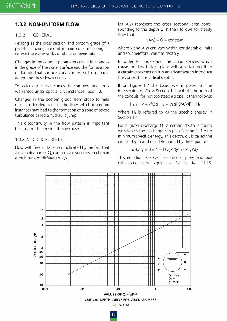
1.3.2.2. CRITICAL DEPTH

Flow with free surface is complicated by the fact that a given discharge, Q, can pass a given cross section in a multitude of different ways.

VALUES OF Q/gD2.5

CRITICAL DEPTH CURVE FOR CIRCULAR PIPES

Figure 1.14

VA

LUES

OF

dc/

D

.0001 .001 .01 .1 1.0

1.0.8

.6

.4

.2

.1.08

.06

.04

.02

.01

Let A(y) represent the cross sectional area corre-sponding to the depth y. It then follows for steady flow that:

vA(y) = Q = constant

where v and A(y) can vary within considerable limits and so, therefore, can the depth y.

In order to understand the circumstances which cause the flow to take place with a certain depth in a certain cross section it is an advantage to introduce the concept 'the critical depth'.

If on Figure 1.7 the base level is placed at the intersection of Cross Section 1-1 with the bottom of the conduit, for not too steep a slope, it then follows:

H1-1 = y + v2/2g = y + 1/2g[Q/A(y)]2 = Hs

Where Hs is referred to as the specific energy in Section 1-1.

For a given discharge Q, a certain depth is found with which the discharge can pass Section 1−1 with minimum specific energy. This depth, dc, is called the critical depth and it is determined by the equation:

dHs/dy = 0 = 1 − Q2/gA3(y) x dA(y)/dy

This equation is solved for circular pipes and box culverts and the results graphed on Figures 1.14 and 1.15.

Q: m3/sD: mg: m/s2

Ddc


13

For uniform flow conditions with given discharge a certain velocity and a certain slope correspond to the critical depth. This velocity and this slope are re-ferred to as the critical velocity and the critical slope respectively. Velocities higher than the critical velocity are supercritical, velocities below are subcritical and flow patterns are referred to as rapid flow (mountain stream) and tranquil flow (river) respectively.

The critical depth occurs in some cross sections near culvert inlets and outlets as dealt with in Section 3.

1.3.2.3 CRITICAL SLOPE

It was mentioned in the previous section that flow under uniform conditions will be rapid or tranquil de-pending on whether the slope is steeper or flatter than the critical slope.

An assessment of critical slopes for part-full flow in concrete conduits indicates that a large proportion will fall into the rapid flow pattern.

This is important when considering the outlet veloci-ties and the possibility of the formation of a hydraulic jump at culvert and drain outlets.

1.3.2.4 THE HYDRAULIC JUMP

In Section 1.3.2.2 it was pointed out that a given discharge can be associated with many different depths of flow. Whichever depth applies in a given cross section depends on the roughness, slope and cross sectional shape not only of the cross section under consideration but also of those adjoining for a considerable length upstream and downstream.

If along the length of the conduit the parameters alter in a manner changing the conditions from supercriti-cal to subcritical the change in depth will take place over a fairly short length and is associated with a con-siderable energy loss. It is referred to as a hydraulic jump and consists of a standing eddy, eddies or waves.

It is of interest to note that although the energy loss caused by the eddies cannot be determined directly it is possible to establish an approximate relationship between the depths before and after the jump.

The turbulence in the eddies has a severe effect on the sides and bottom of the conduit, and it is therefore im-portant to be able to predict where the jump will occur.

VA

LUES

OF

dc(

m)

.1 1 10 100 1000

10080

60

40

20

108

6

4

2

1.0.8

.6

.4

.2

VALUES OF Q/B (m3/sm)

CRITICAL DEPTH CURVE FOR BOX CULVERTS

Figure 1.15

Figure 1.16 TYPICAL HYDRAULIC JUMPS

dc = 0.467 (Q/B)2/3


14

1.4 BOUNDARY SHEAR

The boundary shear is important for questions related to erosion of the conduit wall material and the transport of solids in the water. Traditionally con-trol of both of these effects as well as damage by cavitation has been sought by imposing limitations on flow velocity. Whilst for cavitation the flow velocity is undoubtedly the controlling factor, erosion and transport of solids are better controlled through restrictions on boundary shear.

Using Newton’s second law on a steady, uniform flow situation as illustration on Figure 1.7 shear and grav-ity forces acting on the water prism between cross sections 1 and 2 must be in balance because the pressure forces in the two end sections cancel each other out. Therefore:

PL = ALg sin ALs or

= A s = Rs where P

is boundary shear N/m2

P is wetted perimeter mA is cross sectional area m2

R is hydraulic radius A/P m is density of water kg/m3

g is acceleration due to gravity m/s2

is specific weight of water N/m3

Boundary shear increases approximately with veloc-ity squared, but velocities corresponding to a given shear are larger for large conduits than for small ones. To illustrate the flow velocity − boundary shear relationship for turbulent flow in the transition zone Hf /L from Darcy’s equation in Section 1.2.3.1 is sub-stituted for s in the equation for . The expression can then be written:

= f v2

4 2g

In order to facilitate a comparison between velocity and boundary shear for various relative roughnesses and Reynolds’ numbers this equation is solved graph-ically in Figure 1.17 using for f Colebrook–White’s equation from Section 1.2.3.2.

BOUNDARY SHEAR VERSUS FLOW VELOCITY

Figure 1.17

Re


15

1.5 WATER HAMMER [1.7, 1.8, 1.9]

1.5.1 THE NATURE OF WATER HAMMER

This phenomenon which can result in large increases in the working pressure is caused by a sudden change in the flow rate. The most common causes are the rapid closure of a valve or the sudden stoppage of a pump due to power failure.

Water hammer pressure in metre head is approxi-mately 100 times the velocity change in m/s. That is ha = 100v or a 100 m head for 1 m/s change in velocity.

Reflections of water hammer waves from blank ends, closed valves or reservoirs return the effect to the sys-tem either as an altered velocity or a change in sign of the water hammer pressure. (See Figure 1.18.)

1.5.2 VALVE CLOSURE

In Figure 1.18 (a) the instantaneous closure of a valve makes v go to zero, the head rises by ha and a wave travels from A to B.

Figure 1.18

In concrete pipes the wave travels at a speed of 1000 to 1200 m/s so that after about L/1000 seconds the whole pipe in (b) is expanded a little and the veloc-ity is zero everywhere. The reflection at the reservoir drops the pressure so the pipe returns to normal size and stimulates a negative v (c). In (d) there is − v throughout when the reflection reaches A.

At the closed valve the velocity must return to zero with a corresponding fall of ha and the pipe con-tracts slightly as a wave goes to B as shown in (e).

With another reflection from B in (g) a wave proceeds to A returning the pipe velocity to +v and at the end of 4L/1000 the system is about to repeat the whole process. Energy losses will eventually reduce the value of ha to zero.

Time and magnitude of the change in velocity are both crucial elements in determining the water ham-mer. Reflections can be beneficial and so if the valve closure is longer than 2L/1000 instead of adding water hammer during (a), (b) or (c) above, it is added after (d) and the net result will be less.

This 2L/1000 is a critical time, since total valve closure in less than this time produced the maximum water hammer.

1.5.3 PUMP STOPPAGE

When a pump with an electric motor suffers an un-controlled power failure, inertia effects can help in slowing the process of velocity change but in general a drop in pressure occurs on the delivery side and a rise in pressure occurs on the suction side.

In Figure 1.19 water hammer is just as important on both sides of the pump.

Figure 1.19

The illustration shows that a vacuum can occur with a fall in pressure. Water cannot sustain tension and so a pressure approaching a full vacuum causes vapour to form (separation). The rejoin due to subsequent reflection can produce devastating local water hammer.

First rise

NPump

Pump is subjectto a vacuum

First fall

1.6 REFERENCES

[1.1] D Stephenson, ‘Pipeline Design for Water Engi-neers’, Developments in Water Science, Vol. 6, Elsevier 1976.

[1.2] Design charts for water supply and sewerage. AS 2200:2002.

[1.3] CF Colebrook, ‘Turbulent Flow in Pipes with Particular Reference to the Transition Regional between the Smooth and Rough Pipe Laws’, J Inst Civ Eng 1939, Vol. 11, pp. 133-156.

[1.4] LG Straub, CE Bowers and M Pilch.‘Resistant to flow in two types of concrete pipe’, St Anthony Falls Hydraulic Laboratory. Technical Paper, No. 22, Series B, 1960.

[1.5] AE Bretting ‘Hydraulik’ (in Danish), Copenhagen 1960, p. 241.

[1.6] BA Bakhmeteff, ‘Hydraulics of Open Channels’, Engineering Societies Monograph, McGrath-Hill Book Co, 1932.

[1.7] BB Sharp, E Arnold, ‘Water Hammer – Prob-lems and Solutions’. 1981.

[1.8] J Parmakiain, ‘Water Hammer Analysis’. Dover, 1963.

[1.9] BB Sharp and HR Graze, ‘Water Hammer in Pumping Systems’, Pump Technical Congress, APMA, University of Melbourne, Nov 1980.


16

1.5.4 WAVE SPEED

The water hammer is more precisely

ha = ± Co v

g

Where Co is the wave speed and g acceleration due to gravity.

1 K DK Co = (1 +

eE )and K is the bulk modulus for water (see Section 1.1), its density, D the internal pipe diameter, e the wall thickness and E the elastic modulus for the pipe material, approximately 40,000 MPa.

The above formula ignores a small correction depending on the nature of the pipe support.

STORMWATER RUNOFF SECTION 2

17

SECTION 2

2. STORMWATER RUNOFF

2.1 INTRODUCTION

2.2 RAINFALL 2.2.1 FREQUENCY 2.2.2 POINT MEASUREMENT OF RAINFALL APPLIED TO AN AREA

2.3 PEAK FLOW FORMULA 2.3.1 COEFFICIENT OF RUNOFF 2.3.2 TIME OF CONCENTRATION 2.3.3 LIMITATIONS TO PEAK FLOW FORMULA 2.3.4 TANGENT CHECK

2.4 EXAMPLES 2.4.1 URBAN CATCHMENT 2.4.2 RURAL CATCHMENT 2.4.3 LARGE CATCHMENT

2.5 REFERENCES


18

2.1 INTRODUCTION

Methods of determining the maximum volumes of water to be carried by a stormwater drainage system vary in complexity and difficulty. Depending on the importance of the installation, the safety of life and property, and the degree of inconvenience that may be caused by its inadequacy, the estimate can be a simple matter using basic formulae or just sound judgement or can involve a major scientific and statistical study.

Reviews, methods and comments on their use, are published in [2.1] and [2.2]. This manual deals only with comparatively straightforward circumstances. When more complex conditions occur reference should be made to [2.1], [2.2] and [2.3]. Irrespective of the size and importance of a drainage installation, certain factors should be known and included in the estimate of the design discharge. These factors are given here with methods by which they can be quantified sufficiently accurately for use in relatively simple systems.

2.2 RAINFALL

For any particular location the rainfall is estimated using rainfall intensity-frequency-duration (IFD) data on:

Intensity − mm per hour Frequency − recurrence interval, years Duration − hours

In Australia records of these items are maintained by the Bureau of Meteorology for nearly 500 locations and details can be obtained from the Bureau’s Regional Departments, Municipalities and private organisations and frequently available on request. The rainfall data are used to produce smooth curves of intensity – frequency – duration, examples of which are shown in Figures 2.1 to 2.7.

Note that intensities diminish rapidly as duration increases.

For 100 Australian localities outside the capital cities formulae are available from which intensity – duration graphs may be drawn [2.3].

Outside these areas daily rainfall data will have to be used. The method used for constructing intensity – duration curves depends on the magnitudes of the duration and recurrence interval of the rainfall inten-sity. Maps are provided for these parameters for the whole of Australia in [2.3].

In New Zealand design rainfalls are based on rainfall intensity-frequency-duration (IFD) data. The different sources of this data are given below.

(1) IFD information for a number of rainfall stations throughout New Zealand, for periods from 10 minutes to 72 hours, for Average Recurrence Intervals (ARI’s) of 2, 5, 10, 20 and 50 years, are given in the following reports:

(a) The Frequency of High Intensity Rainfalls in New Zealand – Part I, Water And Soil Tech-nical Publication No. 19 (National Water and Soil Conservation Organisation, Water and Soil Development, MWD, Christchurch, NZ, 1980).

(b) The Frequency of High Intensity Rainfalls in New Zealand – Part II Point Estimates, NZ Met. Serv. Misc. Publ. 162 (Coulter, J.D. and Hes-sell, J.W.D., 1980).

The second report listed above provides IFD information developed from data for a number of automatic rainfall stations throughout New Zealand. The first report provides mapped IFD information derived using the point estimates from the first report. It may be useful for obtaining IFD estimates where there is no rainfall station.

(2) In 1993 NIWA Atmospheric used rainfall data from a large number of gauges (from the start of their records to 1988/89) to develop a computer program, ‘HIRDS – High Intensity Rainfall Design System’. The program allows IFD information for a given location (latitude/longitude) to be obtained for periods from 10 minutes to 72 hours, for Average Recurrence Intervals (ARI’s of 2 to 100 years.

For locations where there is a rain gauge the data is directly related to that gauge, where there is no gauge the program uses an interpolation routine to obtain the IFD point estimates. It also gives standard errors on IFD rainfall estimates which can be used in the rational formula to give upper and lower bound estimates based on rain-fall (if this is required). The program is available for sale from NIWA, who will also provide the IFD tables on a fee for service basis.

(3) IFD data may also be available from a local Regional Council or can be developed (using statistical analysis) from rainfall data obtained from regional Councils or NIWA (previously NZ Meteorological Service).

2. STORMWATER RUNOFF


19

IFD information from the listed sources is for specific point locations. Using this data is reasonable for small catchments less than about 25km2. For larger catch-ments or very complex situations other methods should be used. This manual deals only with compar-atively straight forward circumstances and reviews, descriptions of alternative methods, and comments on their use, are published elsewhere.

IFD tables for Auckland, Wellington, Christchurch and Dunedin are presented in Tables 2.1a-d. It has been supplied by NIWA using the HIRDS program (version 1.03). The data presented is given in mm for the duration being considered (mm/duration). When it is used in the national formula it is very important that the rainfall is converted into mm/hour values for use in the formulas where this is required.

2.2.1 FREQUENCY

The selection of a recurrence interval of the design flood for a drainage system depends on several factors [2.3].

(i) The system will sometimes be surcharged by floods larges than the design flood.

(ii) The design should take into account ultimate development of the catchment area.

(iii) The marginal benefit derived from the systems should equal the marginal cost of providing it. This involves difficult and somewhat subjective calculations and is not always feasible as intan-gible benefits can be involved. The recurrence interval is therefore often a matter of policy rather than calculation.

(iv) All components of a drainage system need not be designed with the same recurrence interval provided that if downstream portions have shorter recurrence intervals the upstream sections are not flooded in consequence.

(v) In the absence of local knowledge or the requirements of supervising authorities and other relevant data, the values in Table 2.1 are a rough guide for use in urban areas.

Table 2.1 RECURRENCE INTERVALS FOR URBAN AREAS[2.4]

When choosing a recurrence interval care should be taken to ensure that potential loss due to flooding is understood and accepted by those responsible for the work.

2.2.2 POINT MEASUREMENTS OF RAINFALL APPLIED TO AN AREA

Principal conditions for which point data may be considered representative of other locations are:

(i) Elevations are within 200 m of each other.

(ii) Annual rainfalls differs by less than 10%.

(iii) Terrains and aspects of the general areas within 5 km of each site are similar.

Type of area Recurrence(ultimate development) interval (years)

Intensely developed business andindustrial where flooding would cause damage or inconvencience 25 to 100

Other business and industrial,developed residential 10 to 25

Sparsely populated residential such as parks, playing fields 5 to 10


Duration (M=min H=hour) 10M 20M 30M 1H 2H 3H 6H 12H 24H 48H 72H

ARI = 2 yrs 9 (1) 13 (2) 17 (2) 24 (3) 33 (3) 38 (3) 50 (5) 63 (6) 80 (8) 99 (10) 110 (11)

ARI = 5 yrs 13 (1) 18 (2) 23 (3) 33 (3) 43 (4) 51 (4) 67 (5) 84 (7) 106 (9) 132 (11) 146 (12)

ARI = 10 yrs 15 (1) 22 (2) 28 (3) 39 (4) 51 (4) 59 (5) 78 (7) 98 (8) 124 (10) 154 (13) 170 (15)

ARI = 20 yrs 17 (2) 25 (3) 32 (3) 45 (5) 57 (5) 67 (6) 88 (8) 111 (10) 141 (13) 174 (16) 193 (18)

ARI = 30 yrs 19 (2) 27 (3) 34 (4) 48 (5) 61 (5) 72 (6) 94 (8) 119 (11) 150 (14) 186 (18) 207 (20)

ARI = 50 yrs 20 (2) 29 (3) 37 (4) 52 (6) 66 (6) 78 (7) 102 (9) 129 (12) 162 (15) 201 (20) 223 (22)

ARI = 60 yrs 21 (2) 30 (3) 38 (4) 54 (6) 68 (6) 80 (7) 104 (10) 132 (12) 167 (16) 207 (21) 229 (23)

ARI = 70 yrs 21 (2) 31 (3) 39 (4) 55 (6) 70 (6) 81 (7) 107 (10) 135 (13) 170 (17) 211 (21) 234 (24)

ARI = 80 yrs 22 (2) 31 (4) 39 (5) 56 (6) 71 (6) 83 (8) 109 (10) 137 (13) 173 (17) 215 (22) 239 (25)

ARI = 90 yrs 22 (3) 32 (4) 40 (5) 57 (7) 72 (6) 84 (8) 110 (10) 139 (13) 176 (18) 219 (23) 242 (25)

ARI = 100 yrs 22 (3) 32 (4) 41 (5) 58 (7) 73 (7) 85 (8) 112 (10) 141 (14) 179 (18) 222 (23) 246 (26)


ARI = 2 yrs 6 (1) 10 (1) 12(1) 18 (2) 26 (2) 31 (3) 43 (4) 59 (5) 82 (8) 102 (10) 113 (11)

ARI = 5 yrs 9 (1) 13 (1) 17 (2) 25 (2) 34 (3) 41 (3) 57 (5) 79 (7) 109 (9) 136 (11) 150 (12)

ARI = 10 yrs 11 (1) 16 (1) 20 (2) 29 (3) 40 (3) 48 (4) 67 (6) 92 (8) 127 (11) 158 (13) 175 (15)

ARI = 20 yrs 12 (1) 18 (2) 23 (2) 33 (3) 45 (4) 55 (5) 76 (7) 105 (9) 145 (13) 180 (16) 199 (18)

ARI = 30 yrs 13 (1) 19 (2) 25 (3) 36 (4) 48 (4) 58 (5) 81 (7) 112 (10) 155 (14) 192 (18) 213 (20)

ARI = 50 yrs 14 (2) 21 (2) 27 (3) 39 (4) 52 (5) 63 (6) 88 (8) 121 (11) 167 (16) 207 (20) 230 (23)

ARI = 60 yrs 14 (2) 21 (2) 28 (3) 40 (4) 54 (5) 65 (6) 90 (8) 124 (12) 172 (17) 213 (21) 236 (24)

ARI = 70 yrs 15 (2) 22 (2) 28 (3) 41 (5) 55 (5) 66 (6) 92 (8) 127 (12) 175 (17) 217 (22) 241 (25)

ARI = 80 yrs 15 (2) 22 (3) 29 (3) 42 (5) 56 (5) 67 (6) 94 (9) 129 (12) 179 (18) 221 (23) 246 (25)

ARI = 90 yrs 15 (2) 23 (3) 29 (3) 42 (5) 57 (5) 69 (6) 95 (9) 131 (12) 181 (18) 225 (23) 249 (26)

ARI = 100 yrs 16 (2) 23 (3) 30 (3) 43 (5) 57 (5) 69 (6) 96 (9) 133 (13) 184 (18) 228 (24) 253 (27)



Table 2.1A. IFD DATA FOR AUCKLAND CITY 36.85S 174.75E (BASED ON DATA FROM 1962 TO 1989)STANDARD ERRORS ARE GIVEN IN BRACKETS. (RAINFALL DEPTHS MM PER DURATION)

Table 2.1B. IFD DATA FOR KELBURN, WELLINGTON 41.28S 174.77E (BASED ON DATA FROM 1928 TO 1989)STANDARD ERRORS ARE GIVEN IN BRACKETS. (RAINFALL DEPTHS MM PER DURATION)

20



ARI = 2 yrs 5 (1) 7 (1) 9 (1) 11 (1) 16 (1) 20 (2) 27 (2) 40 (4) 57 (5) 71 (7) 78 (8)

ARI = 5 yrs 7 (1) 10 (1) 12 (1) 16 (1) 22 (2) 26 (2) 37 (3) 53 (4) 76 (6) 94 (8) 104 (9)

ARI = 10 yrs 8 (1) 11 (1) 14 (1) 19 (2) 25 (2) 31 (3) 43 (4) 61 (5) 88 (7) 110 (9) 122 (10)

ARI = 20 yrs 10 (1) 13 (1) 16 (2) 21 (2) 29 (2) 35 (3) 48 (4) 70 (6) 100 (9) 125 (11) 138 (13)

ARI = 30 yrs 10 (1) 14 (1) 17 (2) 23 (2) 31 (3) 37 (3) 52 (5) 75 (7) 107 (10) 133 (13) 148 (14)

ARI = 50 yrs 11 (1) 15 (2) 19 (2) 25 (3) 33 (3) 40 (4) 56 (5) 81 (7) 116 (11) 144 (14) 160 (16)

ARI = 60 yrs 12 (1) 16 (2) 19 (2) 25 (3) 34 (3) 41 (4) 57 (5) 83 (8) 119 (11) 148 (15) 164 (17)

ARI = 70 yrs 12 (1) 16 (2) 20 (2) 26 (3) 35 (3) 42 (4) 59 (5) 84 (8) 122 (12) 151 (15) 167 (17)

ARI = 80 yrs 12 (1) 16 (2) 20 (2) 27 (3) 36 (3) 43 (4) 60 (5) 86 (8) 124 (12) 154 (16) 170 (18)

ARI = 90 yrs 12 (1) 17 (2) 20 (2) 27 (3) 36 (3) 44 (4) 61 (6) 87 (8) 126(13) 156 (16) 173 (18)

ARI = 100 yrs 12 (1) 17 (2) 21 (2) 27 (3) 37 (3) 44 (4) 62 (6) 89 (8) 128 (13) 158 (16) 175 (19)


ARI = 2 yrs 7 (1) 9 (1) 12 (1) 16 (2) 23 (2) 27 (2) 37 (3) 50 (5) 67 (6) 83 (8) 92 (9)

ARI = 5 yrs 9 (1) 13 (1) 16 (1) 22 (2) 30 (2) 36 (3) 49 (4) 66 (5) 89 (7) 110 (9) 122 (10)

ARI = 10 yrs 11 (1) 15 (2) 19 (2) 26 (2) 35 (3) 42 (4) 57 (5) 77 (6) 104 (9) 129 (11) 143 (12)

ARI = 20 yrs 12 (1) 17 (2) 22 (2) 30 (3) 40 (3) 48 (4) 65 (6) 88 (8) 118 (10) 146 (13) 162 (15)

ARI = 30 yrs 13 (1) 19 (2) 23 (2) 32 (3) 43 (4) 51 (4) 70 (6) 94 (8) 126 (12) 156 (15) 173 (17)

ARI = 50 yrs 14 (2) 20 (2) 25 (3) 35 (4) 46 (4) 55 (5) 75 (7) 101 (9) 136 (13) 169 (17) 187 (19)

ARI = 60 yrs 15 (2) 21 (2) 26 (3) 36 (4) 47 (4) 57 (5) 77 (7) 104 (10) 140 (13) 173 (17) 192 (19)

ARI = 70 yrs 15 (2) 21 (2) 27 (3) 37 (4) 48 (4) 58 (5) 79 (7) 106 (10) 143 (14) 177 (18) 196 (20)

ARI = 80 yrs 16 (2) 22 (3) 27 (3) 38 (4) 49 (4) 59 (5) 80 (7) 108 (10) 145 (14) 180 (18) 200 (21)

ARI = 90 yrs 16 (2) 22 (3) 28 (3) 38 (4) 50 (4) 60 (5) 82 (8) 110 (10) 148 (15) 183 (19) 203 (21)

ARI = 100 yrs 16 (2) 22 (3) 28 (3) 39 (5) 51 (4) 61 (5) 83 (8) 111 (11) 150 (15) 185 (19) 206 (22)



Table 2.1C. IFD DATA FOR CHRISTCHURCH AIRPORT 43.48S 172.53E (BASED ON DATA FROM 1943 TO 1989)STANDARD ERRORS ARE GIVEN IN BRACKETS. (RAINFALL DEPTHS MM PER DURATION)

Table 2.1D. IFD DATA FOR DUNEDIN (MUSSELBURGH) 45.90S 170.52E (BASED ON DATA FROM 1918 TO 1989)STANDARD ERRORS ARE GIVEN IN BRACKETS. (RAINFALL DEPTHS MM PER DURATION)

21


22

11

Hydraulics of Precast Concrete Conduits

SECTION 2

11


SECTION 2

locations on opposite sides of the Great Dividing Range are not similar.

11


SECTION 2


RAINFALL INTENSITY – FREQUENCY – DURATION CURVES FOR

ADELAIDEFigure 2.1


CANBERRAFigure 2.3


BRISBANEFigure 2.2

DURATION h


ADELAIDEFigure 2.1


SECTION 2


DARWINFigure 2.4

11


SECTION 2


11


SECTION 2


11


SECTION 2



23

11


SECTION 2

11


SECTION 2

11


SECTION 2

11


SECTION 2


HOBARTFigure 2.5


MELBOURNEFigure 2.6


PERTHFigure 2.7


SYDNEYFigure 2.8


2424

2.3 PEAK FLOW RATE FORMULA

A common method of estimating a peak flow is the 'Rational Method'.

Q = 2.78 CIAwhere Q = maximum flow rate l/s C = coefficient of runoff A = catchment area ha I = rainfall intensity mm/h for the selected recurrence interval with duration equal to the catchment’s time of concentration, tc (Section 2.3.2).

2.3.1 COEFFICIENT OF RUNOFF

The coefficient of runoff is the fraction of rainfall that becomes runoff. Its value depends on the characteristics of the catchment, e.g. paved city areas, forests, etc. Average coefficients for common characteristics and a range of rainfall intensities are shown on Figure 2.9.

During a rainstorm the actual runoff coefficient in-creases as the soil becomes saturated.

2.3.2 TIME CONCENTRATION

The time of concentration is the maximum time taken by water to travel from within the catchment boundaries to the catchment outlet. When this water reaches the outlet under conditions of uniform rainfall, all the catchment is contributing to the run-off. During a storm of duration shorter than the time of concentration only part of the catchment is con-tributing to the runoff. It is generally assumed that the maximum flow occurs when the rainfall duration equals the time of concentration, hence the use of intensity for duration equal to time of concentration in the peak flow formula. The time required for water to flow over natural surfaces is a function of the nature and the slope of the surface.

For distances up to 1000 m the time of overland flow can be found with sufficient accuracy from the nomogram Figure 2.10.

For larger systems times of concentration should pref-erably be estimated on the basis of locally observed data such as the time of occurrence of flood peaks at or near the catchment outlet compared with the time of commencement of associated storms.

RAINFALL INTENSITY mm/h RAINFALL INTENSITY mm/h RURAL CATCHMENTS URBAN CATCHMENTS

Figure 2.9 [2.3]

1.0

0.9

0.8

0.7

0.6

0.5

0.4

0.3

0.2

0.1

0.00 10 20 30 40 50 60 70 80 90 100 110 120 130 140 150

CO

EFFI

CIE

NT

OF

RU

NO

FF

Steep rocky slopes

1.0

0.9

0.8

0.7

0.6

0.5

0.4

0.3

0.2

0.1

0.00 10 20 30 40 50 60 70 80 90 100 110 120 130 140 150 160 170 180

CO

EFFI

CIE

NT

OF

RU

NO

FF

Clay soil – open crop, close crop or forest

Sandy so

il – fo

rest

Sandy soil –

close cropSandy so

il – open crop

Medium soil – close cropMedium soil – open crop

Parks, l

awns and meadows

Cultivated fi e

lds with good growth

Medium soil – forest

Sand strata

Suburban, fu

lly built-

up on sand

Suburb

an re

sidentia

l with

gardens

Bare loam

Widely detach

ed houses on ordinary loam

Urb

an re

siden

tial, f

ully built-

up with limited gardens

City areas full and solidly built up

Bare

ear

th, e

arth

with

sandsto

ne outcrops

Sem

i det

ache

d houses on bare earth

COm

mer

cial a

nd city areas clo

sely built up

Surf

ace

clay

, p

oor paving, sa

ndstone rock

Impervious roofs, concrete


2525

In the absence of such information recourse may be made to empirical formulae as for instance that of Bransby-Williams [2.3].

Here the overland flow time including the travel time in natural channels is expressed.

tc = __FL__ where

A0.1 s0.2

tc = time of concentration (min)F = a coefficient, 58.5 when area A expressed in km2

= 92.5 when area A expressed in ha L = mainstream length kms = mainstream slope m/km

In urban catchment areas the time of concentration to a drainage inlet is between five and about 30 minutes, and is the sum of:

(a) The time to reach gutters: from roofs – assumed to be five minutes from other runoff areas – see Figure 2.10

(b) The time to flow along the gutter – see Figure 2.11

Gutter flow is normally not significant except in small sub-catchments near the headwater of a catchment area. Pipe flow times may be important. (See Figures 2.10 and 1.10.)

2.3.3. LIMITATIONS TO PEAK FLOW FORMULA

As a general guide to the limitations of the formula Q = 2.78 CIA, its use should be restricted to areas less than 25 km2, but in many parts of Australia there is no practical alternative to its use for much larger areas [2.1], [2.2], [2.3].

2.3.4 TANGENT CHECK [2.5]

It is possible that for a particular urban catchment and assumed recurrence interval and intensity, a more severe storm of shorter duration may not cover the whole area and yet result in a larger flow. Allowance for this possibility can be made by adding a 'Tangent check' to Q = 2.78 CIA.

In general this is only necessary for:

(a) urban catchment areas larger than 15 hectares

(b) significant urban sub-catchments with considerably different times of concentration.

TIME OF TRAVEL OVER SURFACE (min) LENGTH OF OVERLAND FLOW (m)

TIME OF OVERLAND TRAVELFigure 2.10 [2.3]

60 50 40 30 20 10 5 4 3 2 1 5 10 20 50 100 200 500 1000

FLOW DISTANCE L (metres)FLOW IN ‘GUTTERS’

Figure 2.11 [2.4]

Average surfa

ce slopes

0.2%

0.5%

1%2%

5%

10%

20%

Paved surface (n = 0.015)

Bare soil surface (n = 0.0275)

Poorly grassed surface (n = 0.035)

Average grassed surface (n = 0.045)

Densely grassed surface (n = 0.060)


26

2.4 EXAMPLES

2.4.1 URBAN CATCHMENT

Calculate runoff from 0.2 ha of grassed area plus 0.1 ha of paved road contributing to pit A. Recurrence interval – 20 years (Sydney).

tc = time of concentration = t (over land flow) + t (gutter flow). = 14 (Figure 2.10) + 1.7 (Figure 2.11) = 16 min. = 0.27hl20 = (Figure 2.8) 130 mm/hRunoff coefficients:C1 (Figure 2.9):0.50C2 (Figure 2.9):0.90Design discharge to pit A,Q = 2.78 (C1I20A1 + C2I20Ac) = 2.78 (0.5 x 130 x 0.2 + 0.9 x 130 x 0.1) = 69 l/s

2.4.2 RURAL CATCHMENT

Calculate runoff from a 6 ha rural catchment in the Melbourne area. Catchment medium soil, open crop, recurrence interval – five years.

tc (Figure 2.10 – poorly grassed surface) = 24 min = 0.4 hI5 (Figure 2.6) – 45 mm/hC (Figure 2.9) = 0.67Q = 2.78 Cl5A = 2.78 x 0.67 x 45 x 6 = 503 l/s

2.4.3 LARGE CATCHMENT

Determine the peak discharge for use in the design of a highway creek crossing near Sydney. The catch-ment has the following characteristics:

Mainstream length L = 2.5 km Catchment area A = 8.5 km2

Mainstream slope S = 5.4 m/km

Catchment type: Medium soil, close crop.

A recurrence interval of ten years is considered suitable.

From 2.3.2

tc = FL A0.1S0.2

= 58.5 x 2.5 8.50.1 x 5.40.2

= 58.5 x 2.5 = 84 min or 1.40 h 1.24 x 1.40

L10 (Figure 2.8) 45 mm/h Data relating to a locality closer to the site in question may be obtained by referring to [2.3].

C (Figure 2.9) 0.56Peak Discharge Q = 2.78 Cl10A = 2.78 x 0.56 x 45 x 850 = 60,000 l/s

2.5 REFERENCES

[2.1] PJ Colyer and RW Pethick. ‘Storm Drainage Design Methods’, Report No INT 154 March 1976 Hydraulics Research Station, Wallingford, Great Britain.

[2.2] SH Webb and GG O’Loughlin, ‘An Evaluation of Methods used for Design Flood Estimations in NSW’, Local Government Engineering Con-ference 1981.

[2.3] ‘Australian Rainfall and Runoff’, 1977, The Institution of Engineers, Australia.

[2.4] Road Design Manual, Chapter 6, Country Road Board, Victoria, 1974.

[2.5] Urban Road Design Manual, Vol. 2, 1975, Main Roads Department, Queensland.

Pit A

100 m

A2 = 0.1 ha of road pavement

A1 = 0.2 ha grassed area

500 m – Fall 21 mArea 6 ha

50 m at

4% slope Kerb and gutter at 1.5% slope

Slope = 21 x 100 = 4.2% 500

CULVERTS SECTION 3

27

SECTION 3

3. CULVERTS

3.1 INTRODUCTION 3.1.1 TYPES OF CULVERT FLOW CONTROL 3.1.1.1 FLOW WITH INLET CONTROL 3.1.1.2 FLOW WITH OUTLET CONTROL 3.1.1.3 DETERMINATION OF OPERATING CONDITION

3.1.2 HEADWATER 3.1.3 TAILWATER 3.1.4 FREEBOARD

3.2 CULVERTS WITH INLET CONTROL

3.3 CULVERTS WITH OUTLET CONTROL 3.3.1 CULVERTS FLOWING FULL 3.3.2 CULVERTS NOT FLOWING FULL

3.4 FLOW VELOCITY 3.4.1 INLET CONTROL 3.4.2 OUTLET CONTROL 3.4.3 EROSION 3.4.4 SILTATION

3.5 CULVERT SHAPE

3.6 MINIMUM ENERGY CULVERTS

3.7 EXAMPLES 3.7.1 PIPE SOLUTION (INLET CONTROL) 3.7.2 BOX CULVERT SOLUTION (INLET CONTROL) 3.7.3 PIPE SOLUTION (OUTLET CONTROL) 3.7.4 BOX CULVERT SOLUTION (OUTLET CONTROL) 3.7.5 MINIMUM ENERGY CULVERT

3.8 REFERENCES


28

3. CULVERTS

3.1 INTRODUCTION

Road culverts, despite their apparent simplicity, are complex engineering structures from a hydraulic as well as a structural view point [3.5]. Their functional adequacy is no better than the estimate of the design flood, and the hydraulic design described below must be preceded by a careful flood evaluation together with an assessment of the cost resulting from damage caused by design flood being exceeded.

The hydraulic complexity of culverts is a result of the many parameters influencing their flow pattern. This influence can be summarised by referring to two major types of culvert flow.

3.1.1 TYPES OF CULVERT FLOW CONTROL

3.1.1.1 FLOW WITH INLET CONTROL

The culvert flow is restricted to the discharge which can pass the inlet with a given headwater level. The discharge is controlled by the depth of headwater, the cross section area at the inlet and the geometry of the inlet edge. It is not appreciably affected by the length, roughness, slope or outlet conditions and the culvert is not flowing full at any point except perhaps at the inlet. This culvert type is mostly short or steep.

3.1.1.2 FLOW WITH OUTLET CONTROL

The culvert flow is restricted to the discharge which can pass through the pipe and get away from the outlet with a given tailwater level.

The culvert can run full over at least some of its length. The discharge is affected by the length, slope, rough-ness and outlet conditions in addition to the depth of headwater, the cross section area and inlet geometry.

INLET CONTROLFigure 3.1

3.1.1.3 DETERMINATION OF OPERATING CONDITION

It is rarely immediately obvious which pattern of flow a culvert is going to adopt, it is therefore necessary to investigate the consequences of both inlet and outlet control.

The most restrictive of the flow types applies, i.e. the one giving least discharge for given headwater level, or requiring higher headwater level for given discharge.

3.1.2 HEADWATER

Headwater (HW) is the depth of water at the inlet above the invert of the culvert. It is influenced by factors such as:

• acceptable upstream flooding

• pipe flow velocity

• overtopping of the roadway

• possibility of water penetration into the road or rail pavement.

Reference should be made to the appropriate government authorities who have policies on headwater levels and the permissible frequencies and depths of road overtopping.

UNSUBMERGED

WS

WSTW

WSTW

WSTW

SUBMERGEDOUTLET CONTROL

Figure 3.2

CULVERTS SECTION 3

29

3.1.3 TAILWATER

Tailwater (TW) is the depth from the natural water surface at the outlet to the invert of the culvert. The tailwater level may be governed by downstream obstructions or the discharge from other streams.

3.1.4 FREEBOARD

Freeboard is the distance between the headwater level and the crown of the culvert. A minimum is sometimes included in government authority’s poli-cies. [3.1]

3.2 CULVERTS WITH INLET CONTROL

Headwater-discharge relationships are for both pipes and box culverts strongly influenced by inlet geom-etry. [3.4]

Figure 3.3 shows the relationship between diameter, discharge and headwater depth for pipe culverts with square and edged inlet and headwall, socketed inlet and headwall and socketed inlet projecting.

Similarly Figure 3.4 shows the relationship for box culverts and various wing wall angles.

3.3 CULVERTS WITH OUTLET CONTROL

A culvert flowing under outlet control may flow full, full for part of its length or even part full for its entire length as illustrated on Figure 3.2 (a), (b), (c) and (d).

3.3.1 CULVERTS FLOWING FULL

The simplest case of outlet control is illustrated on Figures 3.2(a) and 3.2(b). Here the culvert is flowing full for its entire length. The energy head, H, required to maintain this flow can be expressed:

H = Hv + He + Hf

Where: Hv (velocity head) equals v2/2g

He (energy loss) equals kev2/2g

The entrance loss coefficient ke is given in Table 3.1 for various pipe and box culvert entry conditions and culverts flowing with outlet control.

The entry loss, Hf is ideally calculated from the Colebrook–White equation (see Section 1.2.3.2) but in this particular context the Manning formula has been used because it has been used in [3.4] which forms the basis for most of this chapter.

Figure 3.5 shows the relationship between diameter, discharge and energy head for two different entrance

loss coefficients and the selected value n = 0.011. Similarly Figure 3.6 shows the same relationship for box culverts.

Knowing the energy head H, the headwater, HW, can be calculated from the equation H = HW + Lso – TW when TW is known.

This equation derives from Figure 3.7 and highlights the importance of the tailwater under outlet control.

Table 3.1 [3.4]

ENTRANCE LOSS COEFFICIENT Ke

DESIGN OF ENTRANCE Ke

PIPE CULVERTSPipe projecting from fillsquare cut end 0.5socket end 0.2

Headwall with or without wingwallssquare end 0.5socket end 0.2

Pipe mitred to conform to fill slopeprecast end 0.5field cut end 0.7

BOX CULVERTSNo wingwalls, headwall parallel to embankmentsquare edged on three edges 0.5three edges rounded to 1/12 barrel dimensions 0.2

Wingwalls at 30˚ to 75˚ to barrelsquare edge at crown 0.4crown rounded to 1/12 culvert height 0.2

Wingwall at 10˚ to 30˚ to barrelsquare edge at crown 0.5

Wingwall parallel (extension of sides)square edge at crown 0.7


30

HEADWATER DEPTH FOR CONCRETE PIPE CULVERTSWITH INLET CONTROL

Figure 3.3Adapted from [3.4]

CULVERTS SECTION 3

31

HEADWATER DEPTH FOR BOX CULVERTWITH INLET CONTROL



32

ENERGY HEAD H FOR CONCRETE PIPE CULVERTS FLOWING FULLn = 0.011


NOTE: (a) For a difference value of n, use the length scale shown with an

adjusted length L1 = L (n1/n)2

(b) For a different value of ke connect the given length on adjacent scales by a straight line and select a point on this line spaced

from the two chart scales in proportion to the ke values.

CULVERTS SECTION 3

33

NOTE: (a) For a difference value of n, use the length scale shown with an

adjusted length L1 = L (n1/n)2

(b) For a different value of ke connect the given length on adjacent scales by a straight line and select a point on this line spaced from the two chart scales in proportion to the ke values.

(c) For areas less than 0.3 m2 and boxes with width to height ratios greater than 2 or less than 1, determine H from:

H = [1 + ke + 19.62 n2L] Q2

R4/3 2gA2

ENERGY HEAD H FOR CONCRETE BOX CULVERTS FLOWING FULLn = 0.011



34

dc + D or TW = ho 2

3.3.2 CULVERTS NOT FLOWING FULL

Figure 3.2(c) shows a culvert flowing full for only part of its length and 3.2(d) shows a culvert flowing partly full for its full length.

Both of these flow conditions require complex back-water computations for their rigid analysis, which is beyond the scope of this publication.

CULVERT FLOWING PART FULL

Figure 3.7

However it can be shown that if

dc + D 2

is greater than the tailwater depth, TW, a good approximation for the headwater level can be found by using the charts in Figures 3.5 and 3.6 for full flowing culverts, but substituting

dc + D 2

for TW when calculating HW (for values of d2 refer to Figures 1.14 and 1.15). This approximation is sat-isfactory for normal design purposes if HW > 0.75D. For a more comprehensive approach to the free sur-face flow condition refer to [3.4].

3.4 FLOW VELOCITY

Except when the culverts flow full the highest veloc-ity occurs near the outlet, and this is the point where most erosion damage is likely to occur.

A check on outlet velocity, therefore, must be consid-ered as part of the culvert design.

3.4.1 INLET CONTROL

For culverts flowing with inlet control the outlet velocity can be determined from Figure 1.10 (k = 0.6) in combination with the charts for part full flow Figures 1.12 and 1.13. This approach assumes that the depth of flow at the outlet equals the depth corresponding to uniform flow, but the short length of the average

culvert mostly precludes this, making this approach conservative.

The depth of flow should be checked against critical depth as determined from Figures 1.14 or 1.15.

If flow is supercritical the effect of a hydraulic jump must be considered.

3.4.2 OUTLET CONTROL

For outlet control the average outlet velocity will be the discharge divided by the cross-sectional area of flow at the outlet. This flow area can be either that corresponding to critical depth, tailwater depth (if below the crown of the culvert) or the full cross section of the culvert barrel.

3.4.3 EROSION

Flow of water subjects the conduit material to abra-sion, and too fast a velocity for a given wall material will cause erosion of the conduit. Very fast flows (over 18 – 20 m/s) can cause cavitation unless the conduit surface is very smooth, and this results in erosion taking place at a rapid rate. Cavitation damage does not occur in full flowing pipes with velocities less than about 7.5 – 8 m/s and about 12 m/s in open conduits. [3.10]

Absolute velocities beyond which erosion will take place cannot be given because it depends on factors like smoothness of conduit, quantity and nature of debris discharged and frequency of peak velocity. Commonly adopted values based on experience are listed in Table 3.2.

Table 3.2 [3.1, 3.2, 3.3]

MAXIMUM RECOMMENDED FLOW VELOCITIES,m/s FOR VARIOUS CONDUIT MATERIALS

Precast concrete pipes to AS/NZS 4058 or equal 8.0

Precast box culverts to AS 1597 or equal 8.0

In situ concrete and hard packed rock (300 mm min.) 6.0

Beaching or boulders (250 mm min.) 5.0

Stones (150–100 mm) 3.0–2.5

Grass covered surfaces 1.8

Stiff, sandy clay 1.3–1.5

Coarse gravel 1.3–1.8

Coarse sand 0.5–0.7

Fine sand 0.2–0.5

HW

LSo

HD

L

dc TW

CULVERTS SECTION 3

35

3.4.4 SILTATION

If the flow velocity becomes too low siltation occurs. Flow velocities below 0.5 m/s will cause settlement of fine to medium sand particles, as will be apparent from Table 3.2.

Siltation in culverts mostly occurs if they are placed at incorrect levels, because the flow velocity in the culvert is higher than the average stream flow.

To be self-cleansing they must be graded to the aver-age grade of the water course upstream and down-stream of the culvert, and levels must represent the average stream levels before the culvert was built.

3.5 CULVERT SHAPE

Conventional culvert installation of moderate dis-charge capacity (less than about 25 m3/s) usually have their flow area shaped to fit the natural watercourse as closely as possible.

For such installations a waterway area in m2 of

Q/3 m3/s

can usually be assumed as a first approximation. This area may be provided as single or multiple lines of pipes or box culverts as best suited in each particular case.

Multiple units of equal size are each designed to carry the design flow divided by the number of culvert lines.

3.6 MINIMUM ENERGY CULVERTS

Torrential rains in the coastal regions of Queensland during the monsoon season place heavy demands on road culverts.

In the coastal plains the natural slope of the land is often little more than a fraction of one per thousand which in concrete conduits laid on natural grade, grass covered channels and natural water courses results in tranquil flow (see Section 1.3.2.3).

This has given rise to the development of the concept 'The Minimum Energy Culvert' for use where little fall is available. [3.6]

The aim of 'The Minimum Energy Culvert' concept is to concentrate the flow in a narrow, deep cross section flowing with critical velocity under maximum design flow thus taking advantage of the minimum specific energy under critical flow condition. (Section 1.3.2.2) By keeping the flow outside the supercritical region one avoids the energy loss in a hydraulic jump and the cost of having to protect against the erosion associated with the jump. (Section 1.3.2.4)

The design method is simple but requires knowledge of:

• design discharge

• average natural slope of terrain

• flood levels

• survey details of flood plain adjacent to culvert.

Figure 3.8

Energy line

Water surfaceCulvert and channel bottom

Culvert


36

On the basis of this information a plan and longitudinal section of the culvert is drawn up (Figure 3.8). In doing so the following assumptions are made:

(i) The energy line parallels the natural fall of the terrain.

(ii) Energy losses at entry and exit of culvert are disregarded.

The justification for the latter assumption is that losses at smooth transitions are generally small.

In this context it is worth noting that the exit expan-sion of the stream bed needs to progress at a smaller angle than the entry angle if the formation of stand-ing eddies is to be avoided.

Flow lines and contour perpendicular to these are consequently drawn as smooth curves avoiding sharp angles. The start and finishing levels of the narrowed cross section are those of the natural flood plain.

Using the equations:

Hs,c = 1.5 dc

and Q = b dc g dc

corresponding values of b, dc and Hs can be tried and compared.

The disadvantage of the dip in the longitudinal pro-file can be overcome by a small diameter pipe drain or a channel connecting the culvert to a suitable point downstream.

3.7 EXAMPLES3.7.1 PIPE SOLUTION (INLET CONTROL)

3.7.1.1 DATA

Flow = Q = 5.00 m3/s

Culvert length = L = 90 m

Natural waterway invert levels: Inlet: RL 50.00 m Outlet: RL 49.00 m

Acceptable upstream flood level: RL 52.50

Desirable upstream flood level: RL 52.00

Minimum height of pavement above headwater: 0.30

Required freeboard: Nil

Estimated downstream tailwater level: RL 49.80

(i) Maximum practical culvert height: 52.00 – 0.30 – 50.00 = 1.70 m

(ii) Maximum headwater height, HW, is the lesser of: 52.50 – 50.00 = 2.50 m and (i) above: Maximum HW = 1.70 m

3.7.1.2 ASSUME INLET CONTROL

Enter Figure 3.3 with = 5.00 m3/s and maximum HW = 1.70m.

(i) Try 1650 mm – D = 1.65 m Draw line 1 as shown above and obtain HW/D = 1.09 HW = 1.80 > 1.70 m

(ii) 1800 mm D = 1.8 m Draw line 2 and obtain HW/D = 0.93 HW = 1.67 m But maximum culvert height available is only

1.70 m.

(iii) Twin lines – 2/1050 mm D = 1.05 Q = 2.5 m3/s Draw line 3 and obtain HW/D = 1.62 HW = 1.70 m Use 2/1050 mm diameter pipes

3.7.1.3 CHECK FOR OUTLET CONTROL

Height of tailwater above invert:TW = 49.80 – 49.00 = 0.80 < proposed pipe diameter 1.05 m

Diagram in Figure 3.2(c) depicts actual conditions. Now enter Figure 1.14 to determine critical depth for Q = 2.5 m3/s and D = 1.05 m

Q = 2.5 = 0.71; dc /D = 0.82

gD2.5 9.8 1.052.5

dc = 0.82 x 1.05 = 0.86 m

dc + D = 0.86 + 1.05 = 0.96 >TW = 0.80 2 2 As outlined in Section 3.3.1 enter Figure 3.6 with L = 90 m D = 1050 mm ke = 0.2 (female end of pipe upstream).

Int.

dia

m.

Dis

char

ge

1.62

1.09

0.93

180016501050

(1) (2) (3)

3

1

2

CULVERTS SECTION 3

37

Then use Q = 2.50 m3/s to draw line 2 and obtain H = 1.05 m

Fall of culvert invert, Ls = 50.00 – 49.00 = 1.00 hence:

HW = dc + D + H – Ls = 0.96 + 1.05 – 1.00 = 1.01 m 2HW (inlet control) = 1.70 m greater thanHW (outlet control) = 1.01 m

Inlet control governs.

3.7.1.4 FLOW VELOCITY

For 1050 mm diameter pipes

A = 0.87 m2 and s = 1/90 = 0.011

From Colebrook–White’s Chart for k = 0.6 mm (figure 1.10):

Qf = 3.1 m3/s vf = 3.6 m/s Q/Qf = 2.5/3.1 = 0.81 and from Fig 1.12 v/vf = 1.01 and v = 1.01 x 3.6 = 3.6 m/s y/D = 0.75 and y = 0.75 x 1.05 = 0.79 <dc = 0.86

This means that unless the stream which receives the culvert discharge flows at supercritical flow a hydraulic jump will form at the culvert outlet (see Section 1.3.2.3) and danger of erosion must be checked.

3.7.1.5 SUMMARY

Use 2/1050 mm diameter concrete pipes with female end facing upstream.

Pipes will flow with inlet control with a headwater height of 1.70 m and headwater RL = 51.70 m.

Outlet velocity = 3.6 m/s and the possibility of the formation of a hydraulic jump at the outlet must be checked.

3.7.2 BOX CULVERT SOLUTION (INLET CONTROL)

3.7.2.1

Using the same data as provided for the previous pipe culvert calculate a suitable box culvert size and check for the effects of the outlet velocity.


Enter Figure 3.4 with Q = 5.00 m3/s and max HW = 1.70 m.

Try 1800 x 1200

Q = 5.00 = 2.78 m3/s/m B 1.80

Draw line as shown above and obtain H W/D – 1.25HD = 1.25 x 1.2 = 1.50 < 1.70 m.


TW = 0.8 < 1.2 mEnter Figure 1.15 with

Q = 5.00 = 2.78 m3/s B 1.80

dc = 0.94 m

dc + D = 0.94 + 1.20 = 1.07 >TW = 0.80 m 2 2 As outlined in Section 3.3.1 enter Figure 3.6 with L = 90 m A = 1.2 x 1.8 = 2.16 m2

Ke = 0.5

Draw line 1 and with Q = 5.0 m3/s then line 2 and obtain H = 0.64 m.

Fall of culver invert, Ls = 50.00 – 49.00 = 1.0 m hence:

HW = dc + D + H – Ls 2 = 1.07 + 0.64 – 1.00 = 0.71 m

HW (inlet control) = 1.5 greater than HW (outlet control) = 0.71 Inlet control governs.

Q

D

L

H = 1.05

1

2

ke = 0.2 (1) (2) (3)

HW/DQ/B

2.78 1.25

D

1.2


38

(i) Maximum practical culvert height: 102.5 – 0.5 – 100.0 = 2.0 m

(ii) Maximum headwater height, HW, is the lesser of: 103.0 – 100.0 = 3.0 m And (i) above = 2.0 m Maximum HW = 2.0 m


Enter Figure 3.3 with Q = 0.5 m3/s and max HW = 2.0 m.

Try 450 mm D = 0.45 mDraw line as shown above and obtain: HW/D = 3.5 HW = 3.5 x 0.45 = 1.58 m < 2.0 m


Height of tailwater above invert: TW = 99.8 – 99.0 = 0.80 > 0.45 m

Diagram in Figure 3.2 (a) depicts flow condition, i.e. pipe is flowing full.

Now enter Figure 3.5 with: D = 450 mm L = 120 m Ke = 0.2 (female end of pipe upstream)

Draw line 1

Then use Q – 0.5 m3/m to draw line 2 and obtain H = 3.4 m.

Fall of culvert invert, Ls = 100.0 – 99.0 = 1.00 hence: HW = TW + H – Ls = 0.8 + 3.4 – 1.0 = 3.2 m

Which is unacceptable because HWmax = 2.0 m.

Return to Section 3.7.3.2 using 525 mm pipe diameter in Figure 3.3 and obtain HW/D = 1.9and HW = 1.9 x 0.525 – 1.0 m.

Re-enter Figure 3.5 with D = 525 mm and obtain H = 1.5 hence: HW = 0.8 + 1.5 – 1.0 = 1.3 m.

n 3.7.2.4 FLOW VELOCITY

For 1800 x 1200 A = 1.8 x 1.2 = 2.16 m R = 2.16 = 0.36 2(1.8 + 1.2)

Equivalent D = 4 x 0.36 = 1.44and s = 1/90 = 0.011

From Colebrook-White’s Chart for k = 0.6 mm (Figure 1.10) we get: Vf = 4.4 m/s Qf = 2.16 x 4.4 = 9.5 m3/s

(Note that when using chart for box culverts only D, s, v – relationship can be used. Q must be calculated as Av.)

Q = 5.0 = 0.526 and from Figure 1.13 for B/D = 1.5 Qf = 9.5

v = 1.02 and v = 1.02 x 4.4 = 4.5 m/s vf

y = 0.53 and y = 0.53 x 1.2 = 0.635 < dc = 0.94 m D

Hence the same remark about hydraulic jump applies as made for pipes (Section 3.7.1.4).

3.7.2.5 SUMMARY

Using 1800 x 1200 mm concrete box culvert with square edges.

Culvert will flow with inlet control with a headwater height of 1.5 m and HW RL = 51.5 m.

Outlet velocity = 4.5 m/s and the possibility of hydraulic jump must be checked.

3.7.3 PIPE SOLUTION (OUTLET CONTROL)

Given the following data: calculate a suitable pipe size and check the outlet velocity for the possibility of erosion.

3.7.3.1 DATA

Flow = Q = 0.5 m3/s

Culvert length, L = 120 m

Natural waterway invert levels: Inlet RL = 100.0 m Outlet RL = 99.0 m

Acceptable upstream flood level: RL = 103.0 mDesirable road pavement level: RL = 102.5 mMinimum height of road above headwater: 0.5 mRequired freeboard: NilEstimated downstream tailwater level: RL = 99.8 m

Int.

dia

m.

Dis

char

ge 3.5

0.5 450

(1) (2) (3)

H = 3.4 m

ke = 0.2

Q D

L

2

1

concrete box culvert

CULVERTS SECTION 3

39

This HW is acceptable because 1.3 < HWmax = 2.0 mand since 1.3 > 1.0 = HW (inlet control) outlet control governs.

With HW and TW both well above the crown of the pipe and a moderate slope of 1.0/120 = .0083 the pipe will flow full hence:

v = 4 x 0.5 = 2.3 m/s x 0.5252

which must be checked against erosion danger at outlet (Table 3.2).

3.7.3.4 SUMMARY

Use a single line of 525 mm diameter control pipes with socket end upstream.

The pipe will flow with outlet control and with a HW height of 1.3 m giving a HW RL of 101.3 m and an outlet velocity of 2.3 m/s.

3.7.4 BOX CULVERT SOLUTION (OUTLET CONTROL)

3.7.4.1 DATA

Using the same data as provided for the previous pipe culvert calculate a suitable box culvert size and check for the effects of the outlet velocity.


Enter Fig 3.4 with Q = 0.5 m3/s and HWmax = 2.0 m

Try 600 mm x 300 mmQ/B = 0.5/0.6 = 0.83 m3/smDraw line as shown above and obtain HW/D = 3.6 HW = 3.6 X 0.30 = 1.1m < 2.0 m


TW = 0.80 (see Section 3.73) > 0.30 m hence diagram in Figure 3.2(a) depicts flow condition, i.e. culvert is flowing full.A = 0.6 x 0.3 = 0.18 m2 which is < 0.32 m

...Calculate H from H = 1 + ke + 19.62n2L Q2

R4/3 2gA2

H = 1 + 0.5 + 19.62 x 0.0112 x 120 0.52

= 3.0 0.14/3 2 x 9.81 x 0.182

then HW = TW + H – Ls = 0.8 + 3.0 – 1.0 = 2.8 m.

This is not acceptable because 2.8 > HWmax = 2.0. Try 600 x 375

Inlet control HW will be less than 1.1 m (0.9 m)A = 0.23 which is < 0.3 m2

...Calculate H = 1.65m and HW = 1.45 mThis is acceptable because 1.45 < HWmax = 2.0 and the culvert flows with outlet control since 1.45 m > 0.9 m = HW (inlet control).

As culvert flow full:

v = 0.5 = 2.2 m/s 0.23

3.7.4.4 SUMMARY

Use a single 600 x 375 concrete box culvert with square edges.

The culvert will flow with outlet control with a HW height of 1.45 m giving a HW RL of 101.45 and an outlet velocity of 2.2 m/s.

3.7.5 MINIMUM ENERGY CULVERT

Given a required design flow of 25 m3/s and refer-ring to Figure 3.8 with chosen widths b as set in Table 3.3, calculate suitable levels for the bottom profile of the flared culvert entry at the given sections to achieve critical flow through the culvert. Choose an appropriate box culvert size for the culvert.

Table 3.2 [3.1, 3.2, 3.3]

The widths b are chosen with regard to the survey data, hence q and dc can be calculated for each section.

The depth of flow is required to be critical in the culvert and unchanged subcritical at the start of the flared entry. Intermediate depths are interpolated. For chosen values of d, Hs can be calculated and the

Section 1-1 2-2 3-3

b 14 9 4 q = Q/b 1.79 2.77 6.25

dc = 3q2/g 0.69 0.92 1.58 d 1.10 0.92 1.58 v 1.63 2.13 3.95 v2/2g 0.14 0.23 0.80 Hs 1.24 1.53 2.38

3.6

0.830.30

(1) (2) (3)

D Q/B HW/D


40

bottom level of the culvert and approach is located Hs metre below the energy line in each section. From Table 3.3 it will be noted that a box culvert flow area of 4 m x 1.58 m is required hence a 4.0 m wide x 8.1 m high culvert with a flow area of 7.2 m2 will suffice.

Analysing the problem in the conventional manner as outlined in examples 3.7.2 and 3.7.4, a box culvert flow area of approximately 15 m2 is required.

The conventional approach requires more culvert flow area than the low energy culvert but the latter requires more earthworks and the exit velocity from the culvert is high in comparison to the recommen-dations of Table 3.2 for grass cover.

3.8 REFERENCES

[3.1] Country Roads Boards. Victoria Road Design Manual, 1974.

[3.2] Main Roads Department. Queensland Urban Design Manual, Vol. 2 1979.

[3.3] AE Bretting, Hydraulik (in Danish), Copen-hagen, 1960, p. 428.

[3.4] ‘Hydraulic Charts for the selection of Highway Culverts,’ Hydraulic Engineering Circulars No. 5 & 10, 1965, Bureau of Public Roads, Washing-ton, USA.

[3.5] NH Cottman, KF Porter, JE Tiller, BC Tonkin, ‘A Commentary and Bibliography on the Hydraulics of Culver Design’, ARRB internal report AIR 806-4, 1980.

[3.6] GR McKay, Design of Minimum Energy Culverts, University of Queensland, 1971.

[3.7] Culvert Manual Vol 1, Civil Division Publication 706/A August 1978, Ministry of Works and De-velopment, New Zealand.

[3.8] ‘Hydraulic Design of Energy Dissipators for Culverts & Channels’, US Department of Trans-portation, Hydraulic Circular No. 14.

[3.9] W Bujard (in German), ‘Pipes of Reinforced and non-Reinforced Concrete, Flow, Velocity and Durability’, Tiefbau Vol. 1, 1972.

[3.10] Swedish Building Research Summaries S31: 1976.

STORMWATER DRAINAGE SYSTEMS SECTION 4

41

SECTION 4

4. STORMWATER DRAINAGE SYSTEMS

4.1 INTRODUCTION 4.1.1 HEAD LOSSES 4.1.2 MINIMUM AND MAXIMUM VELOCITIES 4.1.3 TOPOGRAPHY

4.2 RESISTANCE TO FLOW IN CONDUITS 4.2.1 STRAIGHT DRAINS 4.2.2 CURVED DRAINS 4.2.2.1 PIPES 4.2.2.2 BOX CULVERTS

4.2.3 ACTUAL INTERNAL CONDUIT DIMENSIONS

4.3 INLET SHAPE AND CAPACITY

4.4 JUNCTION PITS 4.4.1 INLET PIT WITH INLET FLOW ONLY 4.4.2 JUNCTION PITS WITH INLET AND LATERAL FLOW 4.4.3 OTHER PIT TYPES 4.4.4 INVERT DROP THROUGH PITS

4.5 DEPTH OF DRAINS

4.6 GUTTER FLOW

4.7 STEEP DRAINS

4.8 EXAMPLES 4.8.1 URBAN CATCHMENT UNDERGROUND DRAINAGE 4.8.1.1 DESIGN DISCHARGE

4.8.1.2 DRAIN DESIGN

4.8.2 STEEP SLOPES

4.9 REFERENCES


42

4.1 INTRODUCTION

4.1.1 HEAD LOSSES

The design flow is established as outlined in Section 2, and it is customary in the hydraulic design to assume the pipes flowing full.

The design must take into consideration:

(i) resistance to flow in conduits

(ii) losses at inlets and junction pits, bends and other deviations from straight lines of uniform cross section and flow.

Investigations have shown that the latter source of losses can be of greater significance than the energy losses on uniform straight runs, particularly on short lengths of pipeline [4.1, 4.2].

4.1.2 MINIMUM AND MAXIMUM VELOCITIES

Much of the debris entering stormwater drains is heavier than water, and to ensure some measure of self cleansing a minimum velocity of about 0.5 to 1 m/s at full and half full flow or a boundary shear of 1.5 N/m2 is recommended [4.1, 4.3]. (Refer also to Section 1.4 and 3.4.4.)

Maximum velocities are discussed in Section 3.4.3. Generally velocities should be kept below 8 m/s if possible.

4.1.3 TOPOGRAPHY

Topographic conditions are significant for the design. In very flat country of minimal fall, layout and details minimising head losses are important in order to avoid excessively deep drains.

In hilly country with steep grades design must con-sider the possibility of erosion.

4.2 RESISTANCE TO FLOW IN CONDUITS

4.2.1 STRAIGHT DRAINS

For straight, precast concrete pipes or box culverts flowing full with clean water a k value of 0.15 would be appropriate when using the Colebrook-White equation. Having regard to the effect of the debris a value of 0.6 seems reasonable (Figure 1.10) but it must be realised that no tests under these conditions are known to exist.

4. STORMWATER DRAINAGE Figures 1.8 – 1.11 can be used for box culverts (full or part-full flowing) by substituting 4R for diameter D, where R is the hydraulic radius for the cross section.

4.2.2 CURVED DRAINS

4.2.2.1 PIPES

It is common for drainage pipelines to be laid straight, but there are circumstances when curves or bends are desirable. Concrete pipes can be laid satisfactorily with deflections at the joints to construct curved pipelines with curve radii of 100–300 pipe diameters. Joint deflections range from 0.6 to 3.0˚ dependent on diameter. (See Figure 4.1.)

Splayed pipes and bends can be produced to provide curve radii down to about 5 pipe diameters.

Energy losses in curves formed by joint deflections are only slightly higher than those in straight lines and can be treated as such or an extra allowance of

0.1 v2

2g

can be added for curve deflections over 20˚.

Lobster-back bends show losses with kb –values rang-ing up to 1.3 for 90˚ single splay bends. This and oth-er examples are shown in Table 1.2.

4.2.2.2 BOX CULVERTS

Most box culverts are made with simple butt joints without any claims to watertightness. The joint itself, consequently, offers little scope for joint deflection.

Pipe curves usingpermissible joint

deflections

Deflected sockets

Prefabricated bends

PIPE CURVES AND BENDSFigure 4.1


43

KERB OPENING INLETTYPE E

COMBINATION GRATE AND KERB INLETTYPE G

Section A–A

TYPICAL INLET TYPES

Figure 4.2


44

Splayed joints, however, are incorporated where circumstances require and losses resulting may be estimated from Table 1.2.

4.2.3 ACTUAL INTERNAL CONDUIT DIMENSIONS

Internal dimensions of precast concrete conduits may vary from the nominal dimensions for many reasons. Hydraulic design therefore should be based on actual dimensions of conduits available.

4.3 INLET SHAPE AND CAPACITY

Many forms of drainage inlets leading stormwater from gutters or pavements to adjacent gully pits and underground drainage systems have been devel-oped. Some are grated, some open and others are a combination of the two.

Examples are shown in Figure 4.2. Capacities range from about 20 to 200 l/s and most authorities have developed standard details and information about the types in use in their particular area.

References should be made to these [4.1, 4.7].

4.4 JUNCTION PITS

Underground drainage systems require a multitude of junction pit types to cater for:(i) drainage inlets(ii) inspection(iii) junction of two or more underground drains.

Under peak flood conditions the turbulence in these pits is often considerable and so are the energy losses. These losses must therefore be given careful consideration.

In all instances pit losses are calculated in terms of the velocity head at the pit outlet:

Ho = ko vo2

2g

Ko varies considerably with pit details, but is always positive and mostly in the range 0 to 2.

4.4.1. INLET PIT WITH INLET FLOW ONLY

At the upstream end of most drainage lines is an inlet pit with only an outlet pipe. The energy loss at this point is strongly dependent on the relative depths of water in the pit, as illustrated in Figure 4.3.

RELATIVE DEPTH OF WATER IN INLET d/Do

ENERGY LOSS COEFFICIENT KoFOR INLET FLOW ONLY (BASED ON [4.2])

Figure 4.3

ENER

GY

LO

SS C

OEF

FIC

IEN

T, K

o


45

This water level is assumed to equal the total head at the top of the line, and it must be adequate to over-come both the entry loss and to accelerate the water up to the flow velocity.

In addition it must be far enough below the street level to avoid flooding.

Within these restraints there are still many possibilities and economic considerations will have to be applied in order to reconcile opposing requirements. (i) The top pit must be deep enough to protect the

outlet pipe and to prevent flooding. The deeper it is the lower the pit energy loss and the lower the risk of flooding.

(ii) However, particularly on flat terrain, it is desirable to keep the top pit as high as possible in order to save excavation in the lower region of the system.

4.4.2 JUNCTION PITS WITH INLET AND LATERAL FLOW

The most common types of junction pits are shown diagrammatically on Figure 4.4. Type (a) is a straight through flow pit which can also have an inlet flow. Type (b) is a straight through flow pit with flow en-tering from a lateral. Type (c) is as Type (b) but with provision for inlet flow as well.

In all instances the additional flow enters the pit perpendicular to the direction of the flow passing through the pit.

This entry causes turbulence resulting in the energy losses graphed on Figure 4.5. The graph is derived from [4.2]* and the results are arrived at experimen-tally but they can also be developed theoretically. The lateral flow and top inlet flow are combined and applied as inlet flow only to give a slightly more conservative result but a considerably simpler design procedure.

* Note that ko values graphed in reference [4.2] relate to piezometric or hydraulic pressure loss and not to the energy loss as is common practice and is used throughout this manual.

ENERGY LOSS COEFFICIENT Ko FOR THROUGH-PIT WITH INLET AND LATERAL FLOW

Figure 4.5

Figure 4.4


46

4.4.3 OTHER PIT TYPES

An arrangement where a main is fed by laterals from both sides as in pit type (a) in Figure 4.6 is a possible detail. It should, however, be avoided wherever possible because unless the discharge velocities from L1 and L2 are fairly well balanced the outflow from the lateral with the highest flow velocity is likely to restrict the outflow from the opposite lateral and cause flooding further up that line. Alternative solutions are shown on details (b) and (c).

In general it must be remembered that energy losses through pits are caused by the impact of particles of different velocities and the smoother such transitions are made, the lower the energy loss.

This is of particular importance in flat country where little fall is available.

Figure 4.6

4.4.4 INVERT DROP THROUGH PITS

Particular attention is drawn to the case where on account of change in grade the outlet pipe diameter is smaller than the inlet diameter. Provision must here be made for a drop between pipe inverts of

(1.2 v2o – v2

u ) 2g 2g

to allow for the acceleration of the water.

4.5 DEPTHS OF DRAINS

The depth of the pipes must be such that the head necessary to ensure full flow in the pipes can be accommodated with the water level in all pits remaining below street inlet level. Also the drains must be deep enough to ensure protection of the pipes against traffic loads.

4.6 GUTTER FLOW

A prime requirement is that the design flow will not overtop the gutter. The width also must be limited for the convenience of pedestrians and to avoid the traf-fic hazard caused by water extending into the traffic lane. Design details are shown on Figure 4.7.

4.7 STEEP DRAINS

Drains located on steep slopes must be restrained against the effect of the downwards component of both water and pipe weight.

This component in the direction of the slope can be expressed:

P = [ w D2/4 + c (D + t)t] sin [ w D2/4 + c (D + t)t] s where

t is the wall thickness of the pipe and the angle of the slope.

4.8 EXAMPLES

4.8.1 URBAN CATCHMENT UNDERGROUND DRAINAGE

For the carpark area shown in the diagram below calculate suitable pipe sizes and invert levels for pipes and pits.

ASPHALT CARPARK – ADELAIDE


47

EQUATION: Q + 0.38 (Z/n) S1/2 d8/3

n is Roughness Coeffiecient appropriate to material in bottom of Channel Z is reciprocal of the shoulder cross fall.

(Z/n)S1/2d8/3

NOTES: 1. For shallow V-shaped channel as shown use

nomograph but with Z = T/d2. To determine discharge Qx in portion of channel

having width x: Determine depth d for total discharge in entire

section. Then use nomograph to determine Qb in section of width b for depth d' = d – (x/Z) then Qx = Q – Qb

3. To determine discharge (QT) in composite section: Follow instruction 2 to obtain discharge (Qa) in sec-

tion a at assumed depth d based on an extension of slope ratio Za to intersect water surface: obtain Qc for slopE ratio Z and depth d' = d – x/Za then QT = Qa + Qc

CHANNEL FLOWFLOW IN TRIANIGULAR CHANNELS

Figure 4.7 [4.4]

d d

x x

d' d a

T

b

d'


48

4.8.1.1 DESIGN DISCHARGE

Overland flow distance, ab = 252 = 35 m Slope 1%

Overland flow time (Figure 2.9) 5 min

Assuming pipe flow velocity of 1 m/s pipe flow time for distance bcdef becomes 150/1s = 2.5 min

Time of concentration 7.5 min = 0.125 h

For a recurrence interval of 10 years a rainfall inten-sity of 75 mm/h is obtained from Figure 2.1. With a runoff coefficient of 0.9 (Figure 2.8) the discharges to pits b, g and h then become:

Qb = Qg = Qh = 2.78 CIA = 2.78 x 0.9 x 75 x 0.25 = 47 l/s

And similarly to pits c, d and e.Q2 = Qd = Qe

= 2.78 x 0.9 x 75 x 0.025 = 4.7 l/s

Consequently: Qbc = 47 l/s Qcd = 47 + 5 = 52 l/s Qde = 52 + 47 + 5 = 104 l/s Qef = 104 + 47 5 = 156 l/s

4.8.1.2 DRAIN DESIGN

Calculations proceed from the outfall to the top pit.

Assume: Pipe invert at f : RL 0.000 Total energy head at f : RL 1.000 Pipe diameter e – f : 300 mm

Hence:

Ve–f = Qe–f = 4 x 0.156 = 2.21 m/s

Ae–f x 0.3002

V2e–f = 2.212 = 0.25

2g 19.60 Head loss in e – f (Fig 1.10 – k = 0.6 mm) = (0.02 x 25) = 0.50 m

At pit e: Qo = 156 l/s Qu = 104 l/s Qu/Qo = 0.67

Assuming diameter d – e = 3—mm Do/Du = 1.0 From Fig 4.5 ko = 0.8 hence loss at pit e: 0.8 x 0.25 = 0.20 m

RL energy line just upstream of pit e: 1.00 + 0.50 + 0.20 = 1.70 m

Assume: pipe diameter d – e: 300 mm

head loss in d – e: 0.0085 x 50 = 0.43 mAt pit d: Qo = 104 l/s Qu = 52 l/s Qu/Qo = 0.5

Assuming diameter: c – d = 225 mm Do/Du = 1.33 Hence ko = 1.4

Hence:Head loss at pit d: 1.4 x 0.11 = 0.15 m and RL energy line just upstream of pit d: 1.70 + 0.43 + 0.15 = 2.28 m

Assume: Pipe diameter c – d : 225 mm

Head loss in c – d: 0.0095 x 50 = 0.48 m

At pit c: Qo = 52 l/s Qg + Ql = 52 l/s (see Figure 4.5)

Estimate ko at pit c = 1.5 (sharp 90˚ bend and effect of grate discharge)

Head loss at pit c: 1.5 x 0.09 = 0.14 m hence RL energy line just upstream of pit c: 2.28 + 0.48 + 0.14 = 2.90 m.Assume: Pipe diameter b – c: 225 mHead loss in b – c: 0.0095 x 25 = 0.24 m

RL energy line at b = 2.90 + 0.24 = 3.14 m

If in all instances slope of drains is made equal to line energy losses and pit drops equal to pit energy losses bottom RL of pit b will be 1 m below RL energy line at this point, i.e. 14 (refer to assumption at point f).

Therefore:

And ko = 1.4. Head loss at b < 1.4 x 0.07 = 0.10 m and RL water level at b = 3.14 + 0.10 = 3.24 m which gives a freeboard at the inlet of 0.26 m. The assump-tions made lead to a workable scheme and a longi-tudinal section of the drain may be represented as shown opposite. (Figure 4.8)

For larger schemes it is better to tabulate the calcula-tions. An example of this is shown for the scheme investigated. (Table 4.1)

4.8.2 STEEP SLOPES

Calculate the downward force which must be resist-ed by backfill or anchor blocks for a 1000 mm pipe with a wall thickness of 50 mm on a slope of 1 in 5.

P = x 1/5 (9.8 x ¼ + 24.5 x 1.05 x 0.05) kN/m = 2.35 kN/m (See Section 4.7)


49

PIT

LENGTH DISCHARGE DIAMETER

VELOCITY ENERGY V2/2g

PIT LOSS HEAD I.L. L Q V LINE SLOPE FACTOR ko LOSS

b 1.4 0.10 2.14 25 47 225 1.18 0.0095 0.07 0.24 c 1.5 0.14 1.90/1.16 50 52 225 1.31 0.0095 0.09 0.48 d 1.4 0.15 1.28/1.13 50 104 300 1.47 0.0085 0.11 0.43 e 0.8 0.20 0.70/0.50 25 156 300 2.21 0.02 0.25 0.50 f 0.00

Diameter 225 225 300 300

Final surface

Invert level

Chainage

0

2.14

3.

5

25

1.90

3.

40

1.76

75

1.28

3.

40

1.13

125

0.

70

3.40

0.

50

150

0.

00

3.75

hgb c

d

I.L. g – d 1.90

I.L. h – e 1.90

ef

Table 4.1

Figure 4.8


50

4.9 REFERENCES

[4.1] Urban Road Design Manual Vol. 2, 1975, Main Roads Department, Queensland.

[4.2] WH Sagster, HW Wood, ET Smedon and HC Bossy, Pressure Changes at Storm Drain Junctions, Engineering Series Bulletin No. 1, University of Missouri.

[4.3] Concrete Pipe Handbook,1980 American Con-crete Pipe Association.

[4.4] JR Argue, Urban Surface Drainage Design, ARRB Regional Symposium, Perth 1979.

[4.5] WP Clarke, PJ Strode, JR Argue, Gutter Pavement Flow Relationships for Roadway Channels of Moderate or Steep Grade, Insti-tute of Technology, South Australia, SA Local Government Engineers Conference 1981.

[4.6] BC Tonkin, PK Read, RI Williams, Stormwater Drainage Design Procedure: their efficacy in relation to recent technological advance, Local Government Engineering Conference, August 1981.

[4.7] Road Design Manual, Country Roads Board, Victoria, 1974.

[4.8] ASCE – Manuals and Reports on Engineering Practice – No. 37, Design and Construction of Sanitary and Storm Sewers, New York, 1970.

SEPARATE SEWERAGE SYSTEMS SECTION 5

51

SECTION 5

5. SEPARATE SEWERAGE SYSTEMS

5.1 INTRODUCTION

5.2 THE DESIGN FLOW 5.2.1 DESIGN FLOW COMPONENTS

5.3 GRAVITY SEWERS 5.3.1 MINIMUM GRADE 5.3.2 MAXIMUM GRADE

5.4 THE SEWER DIMENSIONS 5.4.1 ROUGHNESS COEFFICIENT, k 5.4.2 SEWER DESIGN FOR MAXIMUM AND MINIMUM FLOW (GRAVITY) 5.4.3 PUMPING STATIONS AND RISING MAINS 5.4.4. RETICULATION SYSTEMS

5.5 MANHOLES

5.6 CURVES AND BENDS

5.7 DEPTH OF COVER

5.8 OVERFLOWS

5.9 EXAMPLES 5.9.1 GRAVITY TRUNK MAIN 5.9.2 SEWERAGE RETIRCULATION

5.10 REFERENCES


52

5. SEPARATE SEWERAGE SYSTEMS

5.1 INTRODUCTIONIt is a requirement of any sewerage design to comply with local regulations and where necessary the following general guidelines must be modified to ensure such compliance.

5.2 THE DESIGN FLOWFor sewer mains the design flow is usually deter-mined on an area basis for reticulation sewers on a person or household basis.

5.2.1 DESIGN FLOW COMPONENTS

The factors to be considered when establishing the design flow are:

(i) nature of land use (i.e. residential, industrial or commercial

(ii) peak flow relative to mains capacity and possible use of overflow structures

(iii) minimum flow and its effect on the self-cleaning ability of the sewer.

For residential developments the average dry weather flow usually ranges from 200–250 l/person /day, the latter figure corresponding to 'ultimate' development with extensive use of washing machines, etc.

On the basis of the latter figure average conservative sewage discharge rates for residential developments are as show in Table 5.1 and similarly the range of industrial and commercial rates are indicated.

Table 5.1 [5.1, 5.2]

AVERAGE SEWAGE DISCHARGE RATES L/sha

For areas smaller than 40–50 ha average discharge is usually assessed on a person, family or industrial basis.

Peak dry weather discharge in relation to average dry weather discharge is accounted for by multiplying the average flow with a peak factor which is related to area or population to be sewered [5.1].

For catchments up to 40 ha a factor of 3 may be assumed and this may be progressively reduced to 2.5 for areas of around 100 ha.

Wet weather infiltration of stormwater into the sewer system has to be allowed for in the design. It is mostly due to faulty house connections and is therefore considerably higher in old, developed areas than in new ones.

It can be catered for with an additive term of the order given in Table 5.2.

Table 5.2 [5.1]

WET WEATHER INFILTRATION RATES l/sha

The expression for the peak wet weather discharge can now be written:

Q = DWF x d + I (l/sha) where DWF is average dry weather flow d is peak factor I is infiltration allowance.

5.3 GRAVITY SEWERS

5.3.1 MINIMUM GRADE

The presence of suspended matter as well as grit in the sewage and the desire to keep the sewers self-cleansing to the greatest extent possible impose boundary shear or grade restraint on the design. (See Section 1.4.)

Minimum boundary shear for self-cleansing is of the order:

min = 1.3 to 2.5 N/m2 or

Expressed in terms of grade (see 1.4)

smin = 1.3 x 10–4 to 2.5 x 10–4

R R

where R is the hydraulic radius in metres.

RESIDENTIAL (Over 200 inhabitants)Low density 30-45 persons/ha 0.10–0.15Medium density 45-70 persons/ha 0.15–0.25High density 70-150 persons/ha 0.25–0.50

INDUSTRIALNormal average but individual industries 0.25–0.35may rate as high as 10–15

COMMERCIALSuburban business area 0.25–1.5High rise city development 8

Old residential development 0.8–1.2

New residential development 0.4–0.8

New commercial and industrial development 0.1–0.2

sD > 0.0008 m or smin = 0.8/Dmm (self-cleansing)

And sD > 0.0020 m or smin = 2.0/Dmm (slime control)

5.3.2 MAXIMUM GRADE

For plain concrete pipes the same maximum flow ve-locity applies as for stormwater systems, i.e. 8 m/s, but some authorities prefer to keep the velocity well below this value.

In terms of maximum wall shear this corresponds approximately to

max = 150 N/m2 (see Figure 1.17)

or in terms of grade

Smax = 150 x 10–4

R

For PVC lined pipes (see Section 5.4.1) minor dam-age has been known to occur around joint strips if flow velocity exceeded 4.5 m/s. Limiting the veloc-ity to this figure results in the maximum wall shear corresponding approximately to:

Smax = 45 x 10–4

R

This expression is valid for full-flow and part full-flow alike when R-values are used in accordance with Figure 1.12.

The growth of slime on the walls of the sewer has adverse effect on the flow characteristics of the con-duits and produces H2S gas which has a corrosive effect on the concrete. Tests indicate that fast flow-ing sewers are less prone to slime growth than slow flowing ones. Grade control with the objective of limiting slime growth is therefore desirable and wall shear and grades ensuring this are:

min = 3 to 4 N/m2 or

smin = 3 x 10–4 to 4 x 10–4

R R

where the last value applies to rising mains.

Above results are summarised on Figure 5.1 where sD is graphed against Q/QF.

These curves are arrived at by combining the expres-sions for smin corresponding to = 1.35 and 3.4 N/m2 [5.2] for self-cleansing and slime control with the curve for part full flow on Figure 1.12. For Q/QF > 0.2 the minimum grade requirements can be expressed:


53

s = SLOPE m/mD = PIPE DIAMETER

sD

7

6

5

4

3

2

0.0019

8

7

6

5

4

3

2

0.00010 0.2 0.4 0.6 0.8 1.0 Q/QFull

SLOPE DIAMETER LIMITATONS FOR SEWER PIPES

Figure 5.1

Smin Slime control

Smin Self Cleansing


54

For full flowing pipes this can be expressed: sD < 0.060 m or smax = 60/D mm for plain concreteand sD < 0.018 m or smax = 18/D mm for PVC lined concrete

If high velocities are used the flow is often supercritical and attention must be given to the possibility of hydraulic jumps forming where flow is suddenly retarded. Sharp edges also should be avoided in order to prevent cavation.

5.4 THE SEWER DIMENSIONS

5.4.1 ROUGHNESS COEFFICIENT, k (See Section 1.2.3.2)

The special conditions relating to the discharge of sewage as opposed to clean water relate mainly to biological and chemical characteristics of the effluent.

Physically sewage is not much different from clean water but the growth of slime on the sewer surface, caused by its organic content, can influence the roughness appreciably. Tests have indicated rough-nesses up to 6 mm in slimy sewers [5.5], but having regard to the ability of a sufficiently rapid flow to clean off the growth this effect is usually disregarded.

A k-value of 1.5 mm is adopted for design purposes in line with common practice in Australia and Europe [5.1, 5.2, 5.3]. An Australian test series on friction losses in a concrete sewer has given results of the order 0.5–0.7 mm [5.4].

To counter the effect of H2S gas a PVC lining is sometimes used. In centrifugally spun concrete pipes circumferential keys result in longitudinal corruga-tions with a depth of about 3 mm and a pitch of 70.

The effect of this corrugation on the flow resistance has not been experimentally tested but is considered to be similar to that of the joints in unprotected lines; hence no special allowance needs to be made.

5.4.2 SEWER DESIGN FOR MAXIMUM AND MINIMUM FLOW (GRAVITY)

Since two flow conditions impose restraints on the performance, two checks of the design must be made:

(i) the peak wet weather flow(ii) the average dry weather flow.

The sewer dimensions shall be adequate for the first flow conditions with the sewer flowing full and for

the second one flowing part-full with a wall shear adequate to ensure self-cleansing. The overall dry weather flow is important in very flat country, and if the available grade is inadequate to ensure the re-quired wall shear, periodic flushing of the main must be provided for. Flushing may also be necessary in the early stage of a sewerage scheme for a develop-ing area when the ultimate design flows have not yet been reached.

The design for peak flow is carried out using Cole-brook–White’s equation for k = 1.5 (Figure 1.11).

In order to facilitate the check for minimum and maximum flow imposed by cleaning and erosion considerations the grade limits discussed in Section 5.3.1 and 5.3.2 have been superimposed in Figure 1.11. The sewer dimensions can thus be chosen from amongst the possibilities available within the limits here shown.

5.4.3 PUMPING STATIONS AND RISING MAINS

The design flow for pumping stations and rising mains must be established with a balanced view to the environment as well as economy and service. To design small pumping stations for full wet flow is un-economical as this capacity would rarely be used.

Melbourne and Metropolitan Board of Works prac-tice is to provide pumping and main capacity for 4 x DWF. Pumping stations are often provided with wet water by-passes and generally with emergency relief outlets to operate in case of pump breakdown or power failure.

Rising mains are dealt with in Section 6.

5.4.4 RETICULATION SYSTEMS

In the upper reaches of a scheme where only few connections have been made the hydraulic design of the sewer would often lead to diameters too small for practical considerations. Most authorities, therefore, stipulate a minimum which usually is 100–150 mm.

Frequently the design of the smaller diameters (100– 300) is by rule of thumb based on the number of dwell-ings served and the grade of the sewer. Such rules can easily be established on the basis of the above.

5.5 MANHOLESAccess shafts are provided at intervals to gain entry to the sewers for purposes of inspection and mainte-nance. They are usually spaced 100–150 m apart on lines of diameters too small to allow human entry.


55

In lines of larger diameters, the spacing is increased substantially.

In order to reduce the energy losses and the chance of blockage as much as possible the manhole bases are shaped to ensure smooth flow.

Energy losses are as for drainage pits expressed as:

ko v2

2g

where v is the design outlet velocity, and ko the loss factor. The latter is relatively small and can be assumed to range from 0.1–0.4 with the first value corresponding to straight-through manholes and the latter to 90˚ bend ones [5.1].

Mostly the design specifications for major sewerage authorities specify the minimum drops to be provided through the manholes, representative values being as follows:

Straight through manholes – 0.03 m 90˚ bend manholes – 0.08 m

and where outlet diameter is larger than inlet, the minimum drop shall equal the diameter difference with a maximum of 0.25 m [5.2].

Where the outlet diameter is smaller than the entry diameter and an acceleration of flow is necessary, a drop of the order of

(1 + ko) vo

2 – ve

2

m 2g 2g

must be provided.

Ko can be assumed to have values given above.

5.6 CURVES AND BENDS

Curves and bends can be incorporated in sewers in the same manner as outlined for stormwater drains (Section 4.2.2).

5.7 DEPTH OF COVER

Dependant on pipe class, diameter and vehicle load minimum earth covers range between 0.3 and 0.6 m unless special precautions are taken. Demands by other services however may often increase this requirement as may considerations of expansion and contraction of certain soil types under the influence of climatic changes.

Maximum sewer depth depends on the construction technique applied. For sewers constructed in open trenches a maximum trench depth of 6–7 m normally

applies. Deeper sewers are usually constructed in tunnels.

Detailed information about required pipe strength for various depths of the pipes subjected to earth and standard highway loading is determined using the appropriate concrete pipe standards.

5.8 OVERFLOWS

It is common practice to provide overflow structures for sewerage schemes in order to prevent uncon-trolled flooding from manholes and house fittings.

Such overflows are designed to operate in emer-gencies caused by flood water entering the system or breakdowns resulting from blockages or pump failures. Typically they are made to discharge into a stormwater system, but environmental protection regulations must be considered.

5.9 EXAMPLES

5.9.1 GRAVITY TRUNK MAIN

A gravity trunk main has to serve a medium density residential area of 200 ha. Calculate a suitable pie size.

The discharge rate from Table 5.1 is 0.2 l/sha and infiltration rate from Table 5.2 is 0.6 l/sha hence:

Average dry weather flow 0.2 x 200 = 40 l/s, peak wet weather flow 0.2 x 200 x 2.5 + 0.6 x 200 = 220 l/s.

Figure 1.11 gives the following possibilities: 450 @ 0.75% grade 525 @ 0.33% grade 600 @ 0.16% grade

Considering the average dry weather flow as the min-imums for which the main is to be designed, then:

Qmin = 40 = 0.18 QF 220

525 mm is flowing at a velocity slightly less than what would ensure slime control for:

Qmin = 0.20 QF

Unless slime control is required, choose 525 @ 0.33% grade, having regard to the natural surface. If this slopes very steeply the optimum in sewer slope of 300 @ 6% may be acceptable, but beyond this the velocity becomes so high that pipe erosion needs consideration.


56

5.9.2. SEWERAGE RETICULATION

The design discharges for a portion of the layout of a sewerage reticulation system are given in the left hand column of Table 5.2. From this information es-tablish suitable concrete pipe dimensions assuming

Q > 0.2 QF

and self-cleansing.

Table 5.2

MH7 – MH8Figure 1.11 gives the following diameter possibilities: 300 @ 0.82% slope or 225 @ 4.0% slopeSince topography is such that grade must be kept to a minimum in order to save on excavation, 300 @ 0.82% is preferable.

For the drop at MH7 apply the rule for a 90˚ bend from Section 5.5 and adopt 0.08.

MH8 – MH9As for previous section: 450 @ 0.25% or 375 @ 0.68% or 300 @ 1.90%For the same reason as above choose 450 @ 0.25% and a drop at MH8 of 0.15 m.

MH9 – MH10As for the previous MH-length choose the diameter which will handle the flow with the mildest slope giv-ing self cleansing, i.e. 525 @ 0.24%. This solution gives an earth cover of 1.0 m to the pipe at MH10 which in this instance is considered adequate.

MH10 – MH11The slope of the natural surface on this MH-length is 6.28%. At MH 10 the sewer is as shallow as acceptable hence from MH10 to MH11 the line must preferably slope at least as steeply as the natural surface.

From Figure 1.11 it is found that 300 @ 6.28% is more than adequate and acceptable for plain con-crete sewers.

A reduction in diameter from 525 to 300 requires an acceleration from v525 = 0.93 to v300 = 2.83 m/s and in order to avoid the sewage backing up the line from MH10 we must provide a drop at this point of

(1 + ko) v2

300 – v2525

= 1.2 2.832

– 0.932 = 0.44 m

2g 2g 19.6 19.6

The available fall is hence reduced to

10.64 – 0.44 x 100 = 6.01% 577.89 – 408.18

and 300 @ 6.01% becomes a suitable answer.

5.10 REFERENCES

[5.1] International Training Course in Water Supply and Sewerage Practice, Melbourne and Metro-politan Board of Works, 1977.

[5.2] Design of Separate Sewerage Systems, Metro-politan Water Sewerage and Drainage Board Sydney, 1979.

[5.3] The Pipe Handbook, The Danish Concrete Industry (in Danish), 1976.

[5.4] T Clifford, 1978, Head loss measurements on 450 mm sewer rising main, Geelong Water and Sewerage Trust (unpublished).

[5.5] M Johnson, ‘A Literature Review on the Effects of Slime in Sewers’, The British Hydro- mechanics Research Association, Cranfield, Bedford England, 1980.

[5.6] ‘ASCE – Manuals and Reports on Engineering Practice’, No. 37, Design and Construction of Sanitary and Storm Sewers, New York, 1970.

MH Q D s% V IL NS Depth No l/s mm m/s To IL

90 225 2.27 105.41 2.11 7 105.33 107.52 2.19 90 300 0.82 1.27 104.30 4.10 8 108.40 140 450 0.25 0.88

104.15

4.25

9 103.78 109.05 5.27

200 525 0.24 0.93 103.70 5.35

10 103.38 104.96 1.58 200 300 6.01 2.83 102.93 2.02

11 92.74 94.32 1.59

PRESSURE PIPELINES SECTION 6

57

SECTION 6

6. PRESSURE PIPELINES

6.1 INTRODUCTION

6.2 PIPELINE DESIGN 6.2.1 DESIGN INFORMATION 6.2.2 THE DESIGN FLOW (DISCHARGE Q) 6.2.3 ROUGHNESS COEFFICIENT, k 6.2.4 THE PIPE DIAMETER 6.2.5 SLIME GROWTH 6.2.6. MAXIMUM FLOW VELOCITY 6.2.7 THE WORKING PRESSURE 6.2.8 WATER HAMMER GUIDELINES 6.2.8.1 VALVE CLOSURE 6.2.8.2 PUMP LOCATION 6.2.8.3 PUMP START 6.2.8.4 PUMP FAILURE

6.2.8.5 WATER HAMMER PROTECTION

6.2.9 THE FACTORY TEST PRESSURE AND THE EFFECT OF EXTERNAL LOAD 6.2.9.1 REINFORCED CONCRETE PIPES 6.2.9.2 PRESTRESSED CONCRETE PIPES

6.3. THRUST RESTRAINT 6.3.1 CALCULATION OF THRUST 6.3.2 CONCRETE THRUST BLOCKS

6.4 FITTINGS AND VALVES 6.4.1 FITTINGS 6.4.2 VALVES

6.5 FIELD HYDROSTATIC TESTING OF PIPELINES

6.6 EXAMPLES 6.6.1 A PUMPED MAIN 6.6.2 A GRAVITY MAIN 6.6.3 THRUST RESTRAINT 6.6.4 DESIGN FOR PRESSURE AND EXTERNAL LOAD 6.6.5 FIELD TESTING

6.7 REFERENCES


58

6. PRESSURE PIPELINES

6.1 INTRODUCTION

Precast concrete pressure pipes may be used for domestic or industrial water supply, sewerage, irrigation or power station cooling systems.

The pipes are jointed with rubber rings providing flexible joints capable of accommodating ground movements without leaking.

6.2 PIPELINE DESIGN

6.2.1 DESIGN INFORMATION

Before the pipeline can be designed certain basic information is required. It is essential to know:

(i) the required maximum flow (discharge Q)(ii) the longitudinal section(iii) the discharge pressure.

With this information and using the appropriate Colebrook–White chart from Section 1 a suitable pipe size can be determined. Minor losses due to valves, fittings, bends, etc., can be calculated (see Section 1.2.2),

Concrete pressure pipelines should always be buried in the ground in order to protect them against climatic extremes.

An indication of the test pressure ranges which can reasonably be covered by reinforced and prestressed concrete pipes is given in Figure 6.1.

but in supply mains these are usually insignificant. In very short pipelines, however, entry and exit losses may become significant and need to be considered.

6.2.2 THE DESIGN FLOW (DISCHARGE Q)

The relation between design flow, average and peak flow depends on the purpose of the pipeline. If, as in water supply systems, the demand is fluctuating it is common practice to bring the water to a holding reservoir of sufficient capacity to cater for the peak demands. The supply to the reservoir is then main-tained by a pipeline flowing continuously at about average flow. (6.1)

PIPE DIAMETER, mmPRESSURE RANGE – REINFORCED AND PRESTRESSED

CONCRETE PRESSURE PIPES

Figure 6.1


59

The balancing of reservoir capacity and main size is a typical optimisation problem requiring for its solu-tion the relationship between demand and duration of demand.

The domestic water requirement per service can be expressed approximately:

Y (kl/day) = A X–B (1< x <104)

where X is the duration of the demand in hours. A is of the order 10–15 and B 0.2 -0.3. This formula represents a straight line in a double logarithmic plot resembling the rainfall intensity curves (Figures 2.1 to 2.7).

For sewer rising mains the discharge fluctuations are provided for by designing for intermittent operation under average flow conditions and near constant operation under average flow conditions and near constant operation under peak flow. ([6.3] and Section 5.4.4.)

In irrigation work the discharge fluctuations charac-teristic of water supply and sewerage are not present because irrigation mains are designed to meet a constant watering demand. Typical crop require-ments are shown in Table 6.1.

Table 6.1

TYPICAL IRRIGATION REQUIREMENT

With a constant flow 24 hours a day and a known irri-gation area required main capacity can be calculated.

6.2.3 ROUGHNESS COEFFICENT, k

An appropriate value of k must be chosen when using Colebrook–White charts to design concrete pressure pipes (Figures 1.8, 1.9, 1.10).

Test results from measurements on various Australian and overseas concrete pressure pipelines constructed of pipes made by centrifugal spinning of the roller suspension method are listed in Table 6.2.

Of the 7 test series, 5 relate to operating lines and therefore include the effect of some bends and fittings.

Table 6.2ROUGHNESS TESTS

*These tests were carried out on laboratory lines – other lines tested were operating water supply and cooling water lines.

From these results it is concluded that a design value of 0.15 mm is appropriate for concrete pipes flowing full and carrying clean water. This value allows for energy losses caused by fittings normally associated with a supply main.

For sewer rising mains a value of 0.6 mm is recom-mended.

6.2.4 THE PIPE DIAMETER

The pipe diameter necessary to discharge the design flow depends on the head loss acceptable in a given situation.

For gravity mains this is represented by the head available but for pumping mains it is not so simple because a whole range of diameter/pumping heads is technically feasible. The optimum solution will therefore have to be found by considering several alternative schemes.

In each case it is possible to estimate the head, H, necessary to effect the required flow. From Section 1.2.3. H = f Lv2 =f L Q2

D2g D D2

2 2g

4

and the diameter, D, is found from the graphs in Figures 1.8 to 1.10 using the discharge, Q, and the hydraulic gradient H/L.

6.2.5 SLIME GROWTH

An important consideration in pipeline design is the possibility of slime growth on the inside of a pipe-line due to bacterial action. This can cause severe head loss – perhaps more than doubling the original friction loss. Consideration should be given in the pipeline design to the likelihood of swabbing being necessary if this problem occurs and provision made for access to the line for suitable equipment.

Quantity Per Frequency Crop State Watering, of Watering, mm Days

Citrus, Vine Victoria 150 15–21

Sugar Cane Queensland 100 15–peak 30–off peak Cotton Southern Qld Northern NSW 90–100 10

Name of Diameter Roughness Test Line m/m K mm

Liddell Power Station 1690 0.10–0.12 Chicago Test 915 0.005–0.05 Ackers Test 305 0.03–0.06* Barbes Test 800 0.08–0.16 Thai Test 400 0.006–0.08* Perseverance Creek 691 0.09 Rochester, Victoria 450 0.09


60

tc> 10

Lv gH0.25ha

0.75

Where L is the length of the pipeline v the flow velocity and H the total flow energy loss.

For example: L = 500m, v = 2 m/s, H = 5m and ha = 15 m then tc must be at least 90 seconds.

6.2.8.2 PUMP LOCATION

If there is a choice of pump location, then approxi-mately equal lengths of suction and delivery will significantly reduce the water hammer expectation.

6.2.8.3 PUMP START

The working head including water hammer will rarely exceed the shutoff head of the pump provided there is an open delivery point. Trapped air in the pipeline should be avoided at all times as it will contribute to water hammer problems.

6.2.8.4 PUMP FAILURE

In Figure 6.3(a) a classification of pipeline profiles is illustrated as it significantly affects the likelihood of vacuum (separation) conditions on the delivery side after pump failure.

(a) (b)Figure 6.3

Hydraulic pressincluding water hammer

Res. level

p1, p2 and p3 are pipe working pressures correspondingto operating conditions indicated

Pump Flow Flow

HYDRAULIC PRESSURE GRADIENT HYDRAULIC PRESSURE GRADIENT PUMPING MAIN GRAVITY MAIN

Figure 6.2

6.2.6 MAXIMUM FLOW VELOCITY

Economical considerations for pumping mains usually result in flow velocities less than 2 m/s but velocities up to 8 m/s are acceptable where head is available.

6.2.7 THE WORKING PRESSURE

The working pressure is the maximum pressure to which the pipeline will be subjected under operating conditions taking into consideration both steady and fluctuating flow conditions. This pressure will vary along the pipeline and depends on both the longitu-dinal profile of the line and the manner in which it is to be operated.

Water hammer pressures resulting from fluctuations in the operating conditions were introduced in Sec-tion 1.5. Figure 6.2 shows typical longitudinal sec-tions of a gravity main and a pumping main with their operating pressures under steady and fluctuating flow conditions.

6.2.8 WATER HAMMER GUIDELINES (see 1.5)

6.2.8.1 VALVE CLOSURE

If the water hammer resulting from a valve closure is to be kept below a certain value, ha, the closing time tc, for the valve must satisfy the following condition:


61

Profile (iii) is the worst and profile (ii) the best with respect to vacuum conditions. In (b) the pump fail-ure may fall along line AB or AC; both are capable of causing separation but the extent is determined by profile details as in (a). The non-return valve is an essential device which must operate properly. Malfunction produces excess water hammer.

6.2.8.5 WATER HAMMER PROTECTION

Various devices can be used to reduce water hammer pressures, particularly in pumping lines. The principle behind most is to feed water into the line when the pressure begins to drop after a sudden pump stop-page, thus reducing the elastic water hammer effect on the line. In the case of a pump stopping, the initial pressure wave is negative reducing pressure below the hydraulic gradient. The wave changes sign when it returns to the pump the first time and increases the pressure above the hydraulic gradient. If the initial pressure drop can be reduced then the subsequent rise in pressure can also be reduced.

Some devices used for water hammer protection are: flywheels on pumps (pump inertia), a pump bypass with non return valve, surge tanks, discharge tanks, air vessels, inline check valves and automatic pressure release valves [6.4]. The proper use of these devices can significantly reduce water hammer. Obviously the extent to which protection is provided depends on the relative cost of providing it, compared with the cost of designing pipes to withstand the full surge pressure. Detailed analysis is always required.

6.2.9 THE FACTORY TEST PRESSURE AND THE EFFECT OF EXTERNAL LOAD

When establishing the test pressure the effect of both working pressure and external load must be taken into consideration.

6.2.9.1 REINFORCED CONCRETE PIPES

If the pipeline follows the contours of the ground with a nominal cover of about 1 metre, pipes will perform satisfactorily under both pressure and earth load if designed for a minimum test pressure of 1.2 x maximum working pressure (working pressure being defined as the maximum operating pressure includ-ing water hammer effects).

For minor pipelines where no water hammer study is carried out and where consequently only the work-ing pressure applicable to constant operating condi-tions is known a rule of thumb that has being used is:

(i) for gravity mainsFactory test pressure = 1.25 x working pressure or working pressure + 150 kPa, whichever is greater.

(ii) for pumping mainsFactory test pressure = 1.50 x working pressure or working pressure + 150 kPa, whichever is greater.

Although there can be no guarantee that these test pressures will not be exceeded, they include reason-able margins which will cover operating conditions where the line has been properly designed to pre-clude rapid or instantaneous valve closures.

If the external load is considerable due to high fills or heavy traffic loads then the pipe strength may have to be increased to carry this load in combination with the internal pressure; AS/NZS 3725: 2007 provides a method for calculating the hydrostatic test pressure, Pt, and the external test load, T, which when conducted separately are tests of the pipes’ ability to withstand the combined load and pressure.

6.2.9.2 PRESTRESSED CONCRETE PIPES

With prestressed concrete pressure pipes it is usual to design the pipes for various combinations of pressure and external load which take account of long-term loads from working pressures and external load from earth fill, and short-term transient loads from surge pressure and traffic loadings. The usual procedure is to require a factory test pressure which subjects the pipe wall to stresses equivalent to the worst design conditions.

6.3 THRUST RESTRAINT

Concrete pressure pipes with rubber ring joints must be restrained to prevent lateral or longitudinal move-ment and separation of the joints. This must be done wherever these are unbalanced forces such as at bends, reducers, tees and valves. These forces are caused by both pressure and the change in momen-tum of the flowing water. The latter effect is usually ignored as it is very small compared with the pressure component at velocities normally experienced.

6.3.1 CALCULATION OF THRUST

The magnitude of the thrust force due to a change in direction is given by the term:

T = 2pA sin /2 (kN) P = Internal pressure (kPa) A = Cross-sectional area of pipe (m2) = Deflection angle of the bend


62

If the angle of the bend and the pressure are small the thrust is small and the friction drag due to self weight of pipe, water and earth cover combined with the passive resistance of soil against the fitting may be sufficient to balance the forces. If not, thrust blocks will be necessary to resist these forces, which can be very large.

At reducers the pipeline is subjected to longitudinal forces resulting from the change in diameter.

T = p(A1 – A2) (for reducers)

At valves, tees or blank ends similar unbalanced forces occur:

T = pA (for valves, tees and blank ends)

Here also thrust blocks will have to be provided if the forces become too large to be resisted by the backfill alone.

6.3.2 CONCRETE THRUST BLOCKS

The most common method for concrete pipelines is to provide concrete thrust blocks which distribute the load from the fittings over sufficient area to keep the bearing pressure below the safe value for the soil.

Important thrust blocks should be designed using soil mechanics theory so that the line of action of the resisting forces coincides with that of the out of bal-ance pipe thrust. The passive resistance of the soil can be used to resist loads. To develop full passive resistance in soils some movement must take place. For this reason a factor of safety of not less than 2 should be used to allow for water hammer.

The passive soil resistance according to Rankine theory is as follows:

Fp = kp shHL + 2cHLkp

where coefficient of passive earth pressure

= kp = 1 + sin

1 – sin

h = depth of centroid of the thrust block area H = height of the thrust block L = length of the thrust block = soil density cs = soil cohesion

Table 6.2

STRENGTHS OF SOILS TYPICAL VALUES

6.4 FITTINGS AND VALVES

6.4.1 FITTINGS

Fittings are special pipes such as bends, tees, reducers or adaptors which are necessary to accommodate branch lines or valves with various functions.

Fittings can be made from concrete, steel, cast iron or a combination of these materials with final details depending on diameter and pressures.

Small diameter offtakes of low to medium pressure can often be cast into the pipe wall.

Typical examples are shown in Figure 6.5.

Type of Soil Angle of Cohesion Friction N/mm2

Gravel 35˚ 0 Sand 30˚ 0 Silt 28˚ 0.007 Dense clay 5˚ 0.15 Soft saturated clay 0˚ 0.035

REDUCER STEEL OFFTAKE

STEEL SADDLE CONNECTION BEND

SPLAY

TYPICAL FITTINGS

Figure 6.5

BRASS FERRULE REDUCER


63

6.4.2 VALVES

Air valves and scour are usually placed at the peaks and troughs of pressure pipelines in order to facilitate their filling and emptying.

Stop valves are used in various locations to regulate flow and pressure or to isolate sections of a pipeline system.

Check (non-return) valves are usually placed above pumps to prevent backflow in case of power failure or routine stoppage.

Too quick an action by these valves can result in high water hammer pressures. (See Section 6.2.8.1.)

Pressure reducing valves are often used as a water hammer reducing device.

There are many different shapes of each of these valve types, some of them are shown in Fig 6.6.

Figure 6.6

6.5 FIELD HYDROSTATIC TESTING OF PIPELINES

It is usual to pressurise a pipeline on completion as a final acceptance test. This test is to ensure that the pipes have been laid and bedded properly, that joints have been made properly, that pipes have not been damaged during laying and that all associated structures such as valve housings, anchor blocks, etc., perform satisfactorily.

6.6 EXAMPLES

6.6.1 A PUMPED MAIN

A pumping line is required to deliver 600 litres per second from a low level dam to a high level holding reservoir. The length of the line is 5000 metres. The maximum level of the high level reservoir is 150m and the minimum level of the low level dam is 100m. Calculate a suitable pipe size and the head required at the pump.

From Colebrook–White Chart for k = 0.15 (Figure 1.9)Hydraulic gradient required with v = 2.5m/s,

Q = 600 l/sec = 0.85% with pipe diameter = 550 mm.

Using commercial size 600 mm would require gradient of 0.58% at a velocity of 2.2 m per sec.

Head required at pump would be:

150 – 100 m = 50 m (static head)

0.58 x 5000 = 29 m (friction head) 100 2.22 = 0.25 m (velocity head) 2 x 9.8 = 79.25 (total)

If the line had 4 x 90˚ bends and 2 gate valves, calculate the head loss due to these fittings. Using loss coefficients from Table 1.2.

Velocity head = 0.25 m as calculated above90˚ bends – r/D = 1000/600 = 1.67 kb = 0.16Loss = 4 x 0.16 x 0.25 = 0.16 mGrate valves – kv = 0.2 fully openLoss = 2 x 0.2 x 0.25 = 0.10 mTotal loss through fittings = 0.26 m As can been seen the loss due to fittings is of a minor nature and can usually be ignored. The assumed roughness of the pipeline has sufficient allowance for these minor losses.

A 600 mm diameter pressure pipe with a pumping head of 77.25 m would be required.

6.6.2 A GRAVITY MAINA gravity main 3000 m long is required to provide a minimum head of 15 m at the downstream end when flowing at a rate of 400 litres per sec. Minimum level of the storage dam is 120 m and the level of the downstream end is 80 m.

Available hydraulic gradient ignoring minor losses

= 40 – 15 = 0.00833 = 0.833% 3000

AIR VALVE GLOBE VALVE GATE VALVE

CHECK VALVE PRESSURE REDUCING VALVE


64

Using Colebrook–White Chart for Q = 400 l/s and k = 0.15 Figure 1.9

a 500 mm diameter pipe is required, velocity would be 2.5 m/s.

Losses at bends, valves, etc., can be neglected as they are very small. Therefore a 500 mm diameter pipe would be satisfactory.

6.6.3 THRUST RESTRAINTCalculate the size of thrust block to resist the unbal-anced load from a 90˚ bend in a 1200 mm diameter pipeline operating at a pressure of 300 kPa.

Soil properties are = 30˚ (Table 6.2)c = 0.005 mPa. (Table 6.2)s = 19kN/m3

Depth to centre of the thrust block = 3 mOut of balance thrustT = 2 x 300 x /4 x 1.22 sin 45˚ = 480kN

Try an area of 6 m2, L = 3 m, H = 2 m

Angle of friction = 30˚ coefficient of passive earth pressure kp

kp = 1 + sin = 1 + 0.5 1 – sin 1 – 0.5 = 3

Fp = 3 x 19 x 3 x 2 x 3 + 2 x 0.005 x 2 x 3 x 3 x 103

= 1026 + 104 = 1130kN

Factor of Safety = 1130 = 2.35 OK 480

6.6.4 DESIGN FOR PRESSURE AND EXTERNAL LOADA reinforced concrete pressure pipe of 1200 mm diameter is subject to a field external load equivalent to a factory test load W/F of 46 kN/m.

The working pressure (including allowance for surge)

Pw is 450 kPa

The factory test pressure Pt is to be 1.2 times the working pressure (minimum recommended is AS/NZS 3725 – 2007 Design for installation of buried con-crete pipe) = 540 kPa.

The factory test load to allow for combined loading effect: T = W Pt

1/3

F Pt – Pw

= 46 540 1/3

540 – 450

= 46 x 1.82 = 83.6 kN/m

Note: If the external load is the most severe design condition then a more economical design may be chosen by using a larger ratio of Pt /Pw.

6.6.5 FIELD TESTING

Consider the following 1200 mm diameter pipeline.

The pipeline is to be hydrostatically tested in the field to the maximum sustained pressure which equals the static head (gravity line). Calculate the allowable leakage rate for the test. The pipe lengths are 2.5 m.

The number of joints = 5000 2.5

= 2000The average pressure on the line

= 3000 x 40/2 + 2000 x (20/2 + 40/2) 5000

P = 24 m 240 kPa

QL = NdP [6.2] 70 = 2000 x 1.2 240 70 = 531 1/hr

6.7 REFERENCES

[6.1] D Stevenson, 'Developments in Water Science', Pipeline Design for Water Engineers.

[6.2] 'Field Testing of Concrete Pipelines and Joints, CPAA Brochure.

[6.3] 'Design of Separate Sewerage Systems', Metro-politan Water, Sewerage and Drainage Board, Sydney, 1949.

[6.4] ARD Thorley, KJ Everow, Control and Suppression of Pressure Surges in Pipelines and Tunnels, London 1979.

cpaa design manual · pressure pipelines 57 ... hydraulics of precast concrete conduits 3 preface t...

Documents