covid economics - uni-wuppertal.de

COVID ECONOMICS VETTED AND REAL-TIME PAPERS

CHANGING SKILL STRUCTUREElena Mattana, Valerie Smeets and Frederic Warzynski

CAPITAL MARKETS AND POLICIES

Khalid ElFayoumi and Martina Hengge

TRAVEL RESTRICTIONS AND TRADE IN SERVICESSebastian Benz, Frederic Gonzales, Annabelle Mourougane

SOCIAL DISTANCING AND THE POORParantap Basu, Clive Bell and T.Huw

EMERGENCY LOANS AND CONSUMPTION IN IRANMohammad Hoseini and Thorsten Beck

STATE FISCAL RELIEF AND EMPLOYMENT IN THE USChristian Bredemeier, Falko Juessen, Roland Winkler

DEFAULTING ON COVID DEBTWojtek Paczos, Kirill Shakhnov

ISSUE 45 28 AUGUST 2020


Covid Economics Issue 45, 28 August 2020

Copyright: Christian Bredemeier, Falko Juessen, Roland Winkler

Sectoral Employment Effects of State Fiscal Relief: Evidence from the Great Recession, Lessons for the Covid-19 Crisis

Christian Bredemeier1, Falko Juessen2 and Roland Winkler3

Date submitted: 21 August 2020; Date accepted: 22 August 2020

This paper documents that the employment effects of financial aid to U.S. states during the Great Recession were strongly unevenly distributed across sectors. We show that state fiscal relief had a double dividend: not only did it preserve a substantial number of jobs, but it also fostered employment most strongly in the sectors hit hardest by the recession. We exploit differences in the distribution of recessionary job losses across states to draw conclusions for the Covid-19 recession. Our results suggest that the double dividend of state fiscal relief cannot be taken for granted.

1 University of Wuppertal and IZA2 University of Wuppertal and IZA3 University of Antwerp

147C

ovid

Eco

nom

ics 4

5, 2

8 A

ugus

t 202

0: 1

47-1

66


1 Introduction

For state governments in the U.S., the Covid-19 crisis has led to precipitous declines in revenues

and soaring expenses. Since states are effectively required by law to run balanced budgets, many

of them will have to slush costs or raise taxes if not supported financially by the federal govern-

ment. Spending contractions or tax hikes on the part of state governments are likely to deepen

the economic downturn further. Accordingly, there are prominent calls for Congress to provide

financial help to state governments beyond the $150 billion Coronavirus Relief Fund established

in the Coronavirus Aid, Relief, and Economic Security (CARES) Act. The National Governors

Association requested an additional $500 billion in federal aid. The Coronavirus supplemental

spending bill proposed by the Democratic majority in the House of Representatives in May 2020

includes $1 trillion in funding for state and local governments. While Fed Chairman Jerome H.

Powell warned that leaving state governments fight for themselves would make the economic crisis

worse, extending the federal aid to state governments faces powerful opposition from, e.g., Senate

majority leader Mitch McConnel and President Donald Trump.

In this paper, we seek to learn from the Great Recession about the labor-market consequences

of state fiscal relief and to draw conclusions for the Covid-19 crisis. During the Great Recession,

state fiscal relief was one of the major components of the American Recovery and Reinvestment Act

(ARRA), the around $800 billion fiscal stimulus package signed by President Obama in February

2009. The spending component of the ARRA stimulus (which also included about $350 billion in

transfers and tax cuts) was largely channeled through state and local governments who received

close to $250 billion from the federal government. A considerable fraction of this money was

explicitly intended to relax the strain on states’ budgets, and almost all transfers were fungible,

i.e., states could effectively use the money as they wished (Chodorow-Reich et al., 2012, Conley and

Dupor, 2013). Most transfers to states took the form of relieving state governments from payment

obligations, either through increasing federal spending shares in, e.g., Medicaid, or through waiving

states’ cost shares in (e.g., infrastructure) projects financed by the federal government. In both

cases, the respective funds effectively increased states’ budgetary leeway. State fiscal relief has also

been implemented in the course of previous recessions, but the context of the Great Recession is

148C

ovid

Eco

nom

ics 4

5, 2

8 A

ugus

t 202

0: 1

47-1

66


particularly suited to learn about its effects due to the detailed documentation of the outlays.1

Chodorow-Reich et al. (2012), Wilson (2012), Conley and Dupor (2013), and Chodorow-Reich

(2019), among others, have shown that the financial transfers to state governments implemented

in the ARRA had positive employment effects, including substantial effects in the private econ-

omy. In this paper, we look beyond this aggregate effect and study its distribution across sectors.

Specifically, we investigate to what extent state fiscal relief fostered employment in those sectors

that had been hit hardest by the economic downturn. This is important because it is difficult

for workers to switch industries (Weinberg, 2001; Artuc and McLaren, 2015). As a consequence,

promoting employment is particularly valuable in sectors that have been affected severely by the

crisis because this will improve the labor-market prospects of the hardest-hit groups of workers.

From an aggregate perspective, the costs of a recession can be reduced when displaced workers

are enabled to find new jobs in their old industries such that the loss of industry-specific human

capital (Neal, 1995; Sullivan, 2010) are avoided. This is reflected in the statement of purpose of

the ARRA which includes the goals to preserve and create jobs and to assist those most impacted

by the recession.

We build on the approach by Chodorow-Reich (2019) to estimate how the employment effects of

financial aid to states were distributed across sectors. This approach uses pre-recession information

on the size of states’ obligations to avoid endogeneity due to states in worse shape receiving more

federal assistance. We find substantial heterogeneity in the employment effects of state fiscal relief

across sectors. Most strikingly, about 40% of the employment effects (roughly 0.8 out of a total

of 2 job-years per additional $100,000 in aid) materialized in the construction sector, which made

up only about 5.5% of pre-crisis employment. Importantly, we find that the positive employment

effects of transfers to states occurred disproportionately in sectors that were hit harder by the

recession. For example, the construction sector was the sector in which employment had declined

strongest in the early phase of the recession, and our results show that this sector benefitted most

strongly from additional intergovernmental transfers. Hence, state fiscal relief during the Great

1In smaller volume than in the Great Recession, state fiscal relief measures were also implemented in the 1972 Stateand Local Fiscal Assistance Act and the 2003 Jobs and Growth Tax Relief Reconciliation Act. The ARRA includedan unusually strict provision on documentation – section 1512 of the bill requires federal agencies to report outlaysin each state and all prime recipients to report the funds received – as part of President Obama’s transparency andopen government promises.

149C

ovid

Eco

nom

ics 4

5, 2

8 A

ugus

t 202

0: 1

47-1

66


Recession had a double dividend. Not only did it preserve a substantial number of jobs, but it also

protected employment most strongly in the hardest-hit parts of the economy.

We then investigate in how far the double dividend of state fiscal relief can also be expected

in the Covid-19 crisis. This time, most job losses accrued in industries that are characterized

by a high intensity of face-to-face contact between workers and clients such as the leisure and

hospitality sector and retail trade (Adams-Prassl et al., 2020). To shed light on whether extending

state fiscal relief measures would again help most strongly the hardest-hit parts of the economy,

we exploit differences across states in the extent to which the Great Recession hit different sectors

disproportionately. We find that, in states where a specific sector had been hit harder, federal

transfers did not have a significantly more pronounced effect on employment in this sector. This

result hints at the strong employment effects in these sectors, e.g., the construction sector, being

mostly systematic and unrelated to the specifics of the Great Recession. We therefore conclude

that to support the sectors which are hit hardest by the Covid-19 recession, state lawmakers would

have to use intergovernmental transfers in a sharply different way than they did during the Great

Recession.

The remainder of this paper is organized as follows. Section 2 summarizes the econometric

approach, and Section 3 presents the results and discusses the implications of our findings for the

Covid-19 crisis. Section 4 concludes.

2 Methodology

To determine the relationship between the effects of state fiscal relief in a sector and the degree to

which the Great Recession hit the sector, we proceed in two steps. First, we estimate sector-specific

job-year coefficients, i.e., we estimate, sector by sector, the number of additional job-years in this

sector per additional $100,000 of ARRA spending. As discussed in the Introduction, transfers

received through the different programs of the ARRA were essentially alike from the perspective

of a state’s government as they increased budgetary leeway. We therefore analyze the effects of

total ARRA payouts to states. In the second step, we translate the estimated sector-specific job-

year coefficients from the first step into percentage employment effects and regress those on the

percentage job losses before ARRA by sector.

150C

ovid

Eco

nom

ics 4

5, 2

8 A

ugus

t 202

0: 1

47-1

66


To estimate sector-specific job-year coefficients (step 1), we use the Chodorow-Reich (2019)

approach, which exploits variation in ARRA outlays across U.S. states. To address that outlays

were endogenous to a state’s economic condition in the crisis, they are instrumented by states’

pre-crisis payments in domains where the federal government took over parts of the states’ obli-

gations. Chodorow-Reich (2019) has harmonized the instrumental-variable approaches developed

in the literature, and his updated analysis provides a template for studies on the effects of ARRA

intergovernmental transfers. We follow Chodorow-Reich (2019)’s preferred specification and com-

bine three instruments: states’ pre-recession Medicaid spending (as proposed by Chodorow-Reich

et al., 2012), the formulaic component of states’ highway spending (Wilson, 2012; Conley and

Dupor, 2013), and the formulaic component of all ARRA spending by federal agencies allocated

independently of state-specific developments in the recession (Dupor and Mehkari, 2016; Dupor

and McCrory, 2018). For our purpose, it is important that the instruments do not directly affect

the industry mix of employment. The studies cited above carefully demonstrate that funds received

by states through ARRA were fungible, i.e., could be used by state governments as they wished.

This means that, e.g., Medicaid relief did not constitute a stimulus directed to the health sector.

We run separate regressions for each NAICS supersector.2 For supersector i, the baseline

cross-sectional 2SLS regression is given by

H∑h=0

(Ys,i,t+h − Ys,i,t) = αi + βiFs + γ′iXs + εs,i, (1)

with

Fs = Π0 + Π′1Zs + Π′2Xs + νs, (2)

where s denotes federal states, i denotes sectors, and t is the start of the treatment period (in our

case, this is December 2008, when important components of the ARRA became known publicly).

The dependent variable is the cumulated monthly employment level from December 2008 through

December 2010 (by state and sector), net of the level in December 2008, normalized by the adult

2We separate both retail trade and wholesale trade from the trade, transportation, and utilities supersector. Welabel the remaining group of industries in this supersector the transportation, warehousing, and utilities sector. Wefurther separate the manufacturing supersector into durable goods and non-durable goods manufacturing.

151C

ovid

Eco

nom

ics 4

5, 2

8 A

ugus

t 202

0: 1

47-1

66


population, and translated into job-years, i.e.,

Ys,i,t+h − Ys,i,t =1

12

(Employments,i,t+h − Employments,i,t

Working age populations,t

). (3)

Accordingly, the time span is H = 24 months. The endogenous variable Fs is total ARRA outlays

to state s from December 2008 to December 2010, measured in $100,000 increments and per person

of working age in December 2008. It is instrumented by the vector Zs, as described above, where

instruments are normalized by the adult population in December 2008. Following Chodorow-Reich

(2019), we include as control variables (captured in vector Xs) states’ pre-ARRA employment-to-

population ratio as well as pre-ARRA trends in employment and production to account for the

potential threat to identification that states’ differential pre-crisis trends were correlated with the

pre-crisis spending levels measured by the instruments. Specifically, the regressions account for the

December 2008 employment-to-population ratio, the change in employment from December 2007

to December 2008, and the change in gross state product (GSP) from the fourth quarter of 2007

to the fourth quarter of 2008. As in Chodorow-Reich (2019), the control variables are normalized

to have unit variance. In robustness checks, we also control for sector-specific employment trends

within states. The coefficient on ARRA outlays, βi, measures the number of additional job-years in

sector i due to an additional $100,000 spent across all sectors. It compares the actual employment

development in a sector to the counterfactual with fewer ARRA transfers. The approach does not

allow us to disentangle between prevented job destruction and induced job creation. As discussed

by Chodorow-Reich et al. (2012), relief payments were used in two ways: to avoid or alleviate

spending cuts and to prevent or lower tax and fee increases. Accordingly, we phrase our results in

terms of job-years preserved through state fiscal relief.

To determine the relationship between the sectoral employment effects of ARRA transfers to

states and sectoral job losses during the recession (step 2 of our analysis), we calculate, for each

sector i, relative employment gains from an additional $1 billion in yearly ARRA payments,

Gainsi ≡βi · κ

Employmenti,t−13, (4)

where βi · κ with κ ≡ $1 billion/year/$100, 000 is the absolute employment gain from an addi-

tional $1 billion, which we divide by the sector’s pre-crisis employment level in November 2007,

152C

ovid

Eco

nom

ics 4

5, 2

8 A

ugus

t 202

0: 1

47-1

66


Employmenti,t−13. We then regress these relative employment gains on sector-specific relative

employment changes during the first year of the recession (i.e., the part of the downturn before

ARRA):

Gainsi = δ + ζ ·Employmenti,t−1 − Employmenti,t−13

Employmenti,t−13+ εi. (5)

To take into account estimation uncertainty from step 1, we weigh observations by the statistical

significance (one minus p-value) of the estimated job-year coefficients βi. This regression does not

aim at identifying a causal relation between recessionary job losses and the sectoral effects of the

ARRA, but it is merely an accounting tool that helps to summarize the descriptive relationship

between the two.3

Data. Monthly employment data by state and industry come from the Current Employment

Statistics (CES) of the Bureau of Labor Statistics (BLS).4 For a few sector-state combinations, the

required monthly employment information is missing (see Table A.1 in the Appendix for sample

sizes). We use the data on ARRA outlays and the instruments from Chodorow-Reich (2019).

Population data are from the BLS Local Aea Unemployment Statistics and GSP data are from the

Bureau of Economic Analysis (BEA) Regional Data, GDP by state.5

3 Results

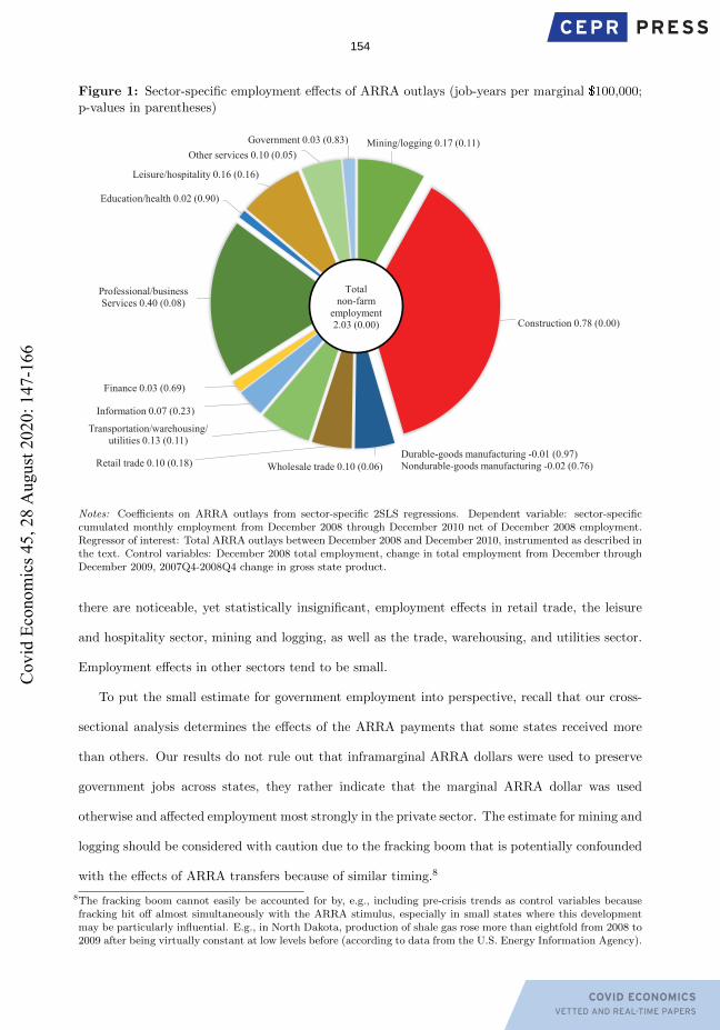
Sector-specific employment effects. The results from the first step of our analysis are sum-

marized in Figure 1, which displays the estimated sector-specific job-year coefficients (the full

regression results are shown in Table A.1 in the Appendix).6 As Chodorow-Reich (2019), we esti-

mate that an additional $100,000 in ARRA payouts increased total employment by the equivalent

of about two jobs, each of which lasts for one year.7 Figure 1 illustrates that there was substantial

heterogeneity in the effects across sectors. Close to 0.8 job-years, or nearly 40% of the total im-

pact, accrued in the construction sector. Professional and business services, wholesale trade, and

the residual “other services” sector also experienced significant employment effects. Furthermore,

3As emphasized in Chodorow-Reich et al. (2012), it is unlikely that employment developments until November 2008already reflected anticipated effects of the ARRA stimulus. Important components of the ARRA became apparentno sooner than in December 2008.

4See https://www.bls.gov/sae/data/home.htm5See https://www.bls.gov/lau/ and https://www.bea.gov/data/gdp/gdp-state, respectively.6First-stage F-statistics range from 39.8 to 46.1.7The difference between our estimate (2.03) and Chodorow-Reich (2019)’s estimate (2.01) is due to data revisions.

153C

ovid

Eco

nom

ics 4

5, 2

8 A

ugus

t 202

0: 1

47-1

66


Figure 1: Sector-specific employment effects of ARRA outlays (job-years per marginal $100,000;p-values in parentheses)

Mining/logging 0.17 (0.11)

Construction 0.78 (0.00)

Wholesale trade 0.10 (0.06)Retail trade 0.10 (0.18)

Transportation/warehousing/utilities 0.13 (0.11)

Information 0.07 (0.23)

Finance 0.03 (0.69)

Professional/business Services 0.40 (0.08)

Education/health 0.02 (0.90)

Leisure/hospitality 0.16 (0.16)

Other services 0.10 (0.05)Government 0.03 (0.83)

Durable-goods manufacturing -0.01 (0.97)Nondurable-goods manufacturing -0.02 (0.76)

Total non-farm

employment 2.03 (0.00)

Notes: Coefficients on ARRA outlays from sector-specific 2SLS regressions. Dependent variable: sector-specificcumulated monthly employment from December 2008 through December 2010 net of December 2008 employment.Regressor of interest: Total ARRA outlays between December 2008 and December 2010, instrumented as described inthe text. Control variables: December 2008 total employment, change in total employment from December throughDecember 2009, 2007Q4-2008Q4 change in gross state product.

there are noticeable, yet statistically insignificant, employment effects in retail trade, the leisure

and hospitality sector, mining and logging, as well as the trade, warehousing, and utilities sector.

Employment effects in other sectors tend to be small.

To put the small estimate for government employment into perspective, recall that our cross-

sectional analysis determines the effects of the ARRA payments that some states received more

than others. Our results do not rule out that inframarginal ARRA dollars were used to preserve

government jobs across states, they rather indicate that the marginal ARRA dollar was used

otherwise and affected employment most strongly in the private sector. The estimate for mining and

logging should be considered with caution due to the fracking boom that is potentially confounded

with the effects of ARRA transfers because of similar timing.8

8The fracking boom cannot easily be accounted for by, e.g., including pre-crisis trends as control variables becausefracking hit off almost simultaneously with the ARRA stimulus, especially in small states where this developmentmay be particularly influential. E.g., in North Dakota, production of shale gas rose more than eightfold from 2008 to2009 after being virtually constant at low levels before (according to data from the U.S. Energy Information Agency).

154C

ovid

Eco

nom

ics 4

5, 2

8 A

ugus

t 202

0: 1

47-1

66


Figure 2: Employment effects of ARRA outlays by sector’s exposure to downturn.

-10 -8 -6 -4 -2 0 2 4

employment change, 11/2007-11/2008 (% of pre-crisis)

-0.4

-0.2

0

0.2

0.4

0.6

0.8

1

1.2

emp

loy

men

t ef

fect

of

$1

B a

id t

o s

tate

s (%

of

pre

-cri

sis)

Construction

Durable goods

Non-durable goods

WholesaleRetail

TWU

Information

Finance

Prof./bus. serv.

Education/health

Leisure/hospitality

Other services

Government

Total

Goods-producing industries

Service-providing industries

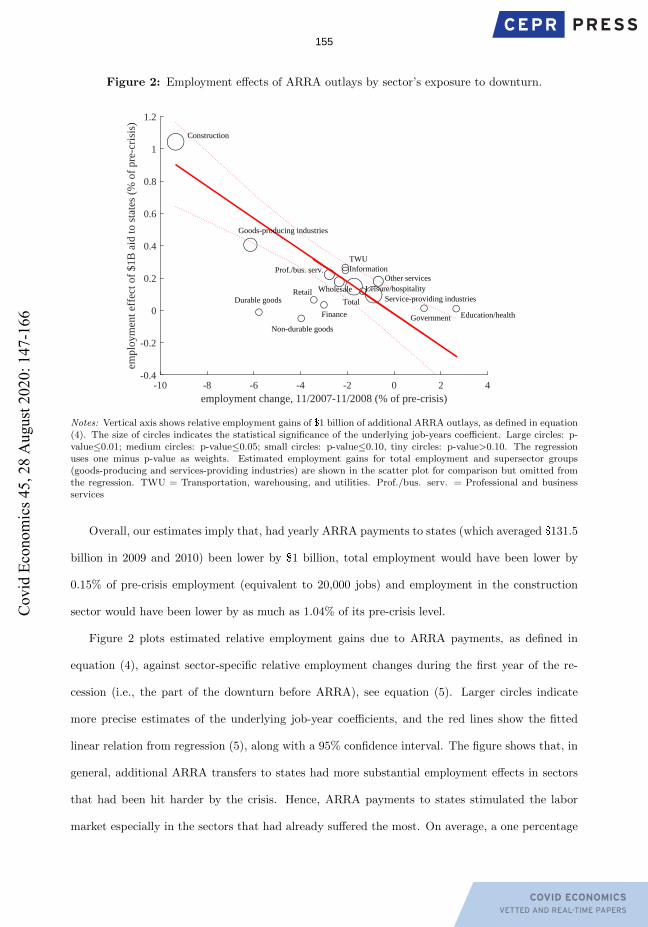
Notes: Vertical axis shows relative employment gains of $1 billion of additional ARRA outlays, as defined in equation(4). The size of circles indicates the statistical significance of the underlying job-years coefficient. Large circles: p-value≤0.01; medium circles: p-value≤0.05; small circles: p-value≤0.10, tiny circles: p-value>0.10. The regressionuses one minus p-value as weights. Estimated employment gains for total employment and supersector groups(goods-producing and services-providing industries) are shown in the scatter plot for comparison but omitted fromthe regression. TWU = Transportation, warehousing, and utilities. Prof./bus. serv. = Professional and businessservices

Overall, our estimates imply that, had yearly ARRA payments to states (which averaged $131.5

billion in 2009 and 2010) been lower by $1 billion, total employment would have been lower by

0.15% of pre-crisis employment (equivalent to 20,000 jobs) and employment in the construction

sector would have been lower by as much as 1.04% of its pre-crisis level.

Figure 2 plots estimated relative employment gains due to ARRA payments, as defined in

equation (4), against sector-specific relative employment changes during the first year of the re-

cession (i.e., the part of the downturn before ARRA), see equation (5). Larger circles indicate

more precise estimates of the underlying job-year coefficients, and the red lines show the fitted

linear relation from regression (5), along with a 95% confidence interval. The figure shows that, in

general, additional ARRA transfers to states had more substantial employment effects in sectors

that had been hit harder by the crisis. Hence, ARRA payments to states stimulated the labor

market especially in the sectors that had already suffered the most. On average, a one percentage

155C

ovid

Eco

nom

ics 4

5, 2

8 A

ugus

t 202

0: 1

47-1

66


point stronger decline in employment during the first year of the recession is associated with a

roughly 0.1 percentage points stronger estimated employment effect of an additional $1 billion in

ARRA outlays (i.e., ζ = 0.099, p-value<0.001).9 This reveals the double dividend of state fiscal

relief in the Great Recession: many jobs were preserved, and disproportionately so in sectors that

were affected disproportionately by the downturn. This way, state fiscal relief prevented further

deterioration of the labor-market prospects of the hardest-hit groups of workers.

We corroborated our results in several robustness checks. In particular, we applied the Medicaid

instrument suggested by Chodorow-Reich et al. (2012) rather than the baseline combination of

instruments controlled for sector-specific pre-ARRA employment trends, and accounted for the full

set of control variables considered in Chodorow-Reich (2019)’s sensitivity analysis. See Appendix

for details.

Lessons for the Covid-19 crisis. While the Great Recession was a typical recession regarding

the distribution of job losses across sectors with construction and manufacturing being the hardest-

hit sectors (Hoynes et al., 2012), the Covid-19 crisis is different. This time, other sectors are most

strongly affected by the downturn, such as retail trade, leisure, and hospitality. We now discuss

whether extending financial aid to states in the Covid-19 crisis would also yield a double dividend

in the sense that the additional funds would save or create jobs disproportionately in the sectors

that are hit hardest by this recession. One the one hand, we have documented that the overall

employment gains due to state fiscal relief during the Great Recession were moderate in those

sectors that are now hit hard by the Covid-19 crisis, see Figure 1. On the other hand, we have

shown that, during the Great Recession, there was a positive relationship between the employment

gains due to state fiscal relief and how strongly a sector was affected by the downturn, see Figure

2. If the latter finding applies to recessions in general, we can expect that extending state fiscal

relief in the Covid-19 crisis would support employment predominantly in the hardest-hit parts of

the economy, in particular retail trade, leisure, and hospitality. To shed light on this, we exploit

that, in the Great Recession, the distribution of job losses across sectors differed between states.

For example, in the first twelve months of the Great Recession, the construction sector in the U.S.

9In line with our previous results, the construction sector is an important driver of this result, being the sector mostaffected by the crisis and the strongest beneficiary of the relief money. Leaving out this sector weakens the relationbetween crisis exposure and employment effects of ARRA outlays, but the relationship continues to be negative.

156C

ovid

Eco

nom

ics 4

5, 2

8 A

ugus

t 202

0: 1

47-1

66


was about six percentage points more affected by job losses than the U.S. economy as a whole.

In New York State and Texas, however, job losses in the construction sector were less than two

percentage points higher than the drop in total employment in these states, while in California and

Florida, they were over 11 percentage points higher than the state-specific average. Exploiting this

variation between state-specific recessions allows us to investigate how the distribution of job losses

in a downturn affects the distribution of the effects of state fiscal relief. Our empirical approach is

to examine whether a particular sector tended to benefit more strongly from ARRA payments in

those states where it had previously suffered more severely from the crisis. If this is the case, then

it can be concluded that systematic forces ensured that specific sectors benefited strongly from the

ARRA payments because they had been strongly affected by the crisis. Then, we may expect the

double dividend of state fiscal relief to occur also in the Covid-19 crisis.

Technically, we consider an additional set of regressions where we interact ARRA payouts with

the pre-ARRA drop in sector-specific employment relative to total employment. We define, for each

sector i in each state s, a measure of the excess exposure to the downturn in 2007/08 as the percent

employment change for sector i in state s between December 2007 and December 2008 minus the

percent change in total employment in state s, and normalize this variable to have mean zero

and variance one. Our baseline empirical model (1) is then augmented by the interaction between

ARRA outlays and the excess-exposure measure, and the excess-exposure measure further enters

the second stage as an additional control variable. Here, we use the three instruments from the

baseline regressions as well as their respective interactions with the excess exposure measure as

instruments (giving a total of six instruments) to instrument ARRA outlays and the interaction

term.

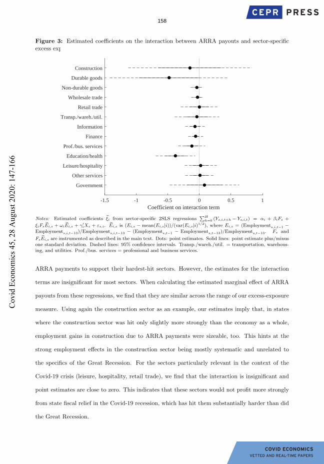
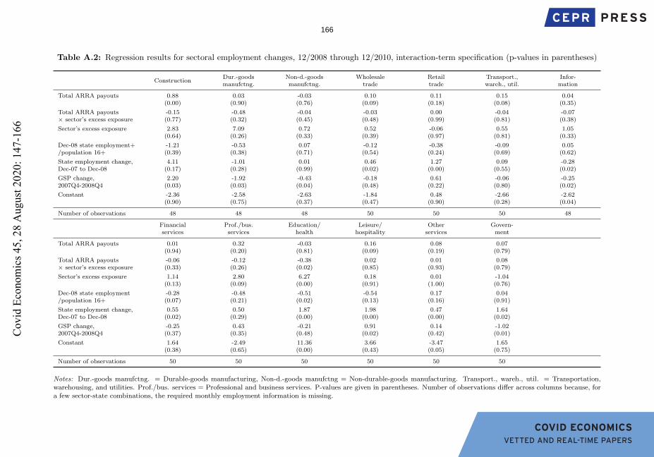
Figure 3 illustrates the estimated coefficients on the interaction terms in the sector-specific

regressions (the full regression results are documented in Table A.2 in the Appendix). In most

sectors, the estimated coefficient on the interaction term is negative. This result implies that,

in states where the respective sector was hit harder by the Great Recession, ARRA transfers to

this state tended to have a more substantial effect on employment in this sector. The strong

employment effects in the construction sector may thus partly result from this sector’s significant

exposure to the crisis, for example, because state governments deliberately decided to use the

157C

ovid

Eco

nom

ics 4

5, 2

8 A

ugus

t 202

0: 1

47-1

66


Figure 3: Estimated coefficients on the interaction between ARRA payouts and sector-specificexcess exposure to the Great Recession.

-1.5 -1 -0.5 0 0.5 1

Coefficient on interaction term

Government

Other services

Leisure/hospitality

Education/health

Prof./bus. services

Finance

Information

Transp./wareh./util.

Retail trade

Wholesale trade

Non-durable goods

Durable goods

Construction

Notes: Estimated coefficients ξi from sector-specific 2SLS regressions∑H

h=0 (Ys,i,t+h − Ys,i,t) = αi + βiFs +

ξiFsEi,s + ωiEi,s + γ′iXs + εs,i. Ei,s is (Ei,s − mean(Ei,s|i))/(var(Ei,s|i)1/2), where Ei,s = (Employments,i,t−1 −Employments,i,t−13)/Employments,i,t−13 − (Employments,t−1 − Employments,t−13)/Employments,t−13. Fs and

FsEi,s are instrumented as described in the main text. Dots: point estimates. Solid lines: point estimate plus/minusone standard deviation. Dashed lines: 95% confidence intervals. Transp./wareh./util. = transportation, warehous-ing, and utilities. Prof./bus. services = professional and business services.

ARRA payments to support their hardest-hit sectors. However, the estimates for the interaction

terms are insignificant for most sectors. When calculating the estimated marginal effect of ARRA

payouts from these regressions, we find that they are similar across the range of our excess-exposure

measure. Using again the construction sector as an example, our estimates imply that, in states

where the construction sector was hit only slightly more strongly than the economy as a whole,

employment gains in construction due to ARRA payments were sizeable, too. This hints at the

strong employment effects in the construction sector being mostly systematic and unrelated to

the specifics of the Great Recession. For the sectors particularly relevant in the context of the

Covid-19 crisis (leisure, hospitality, retail trade), we find that the interaction is insignificant and

point estimates are close to zero. This indicates that these sectors would not profit more strongly

from state fiscal relief in the Covid-19 recession, which has hit them substantially harder than did

the Great Recession.

158C

ovid

Eco

nom

ics 4

5, 2

8 A

ugus

t 202

0: 1

47-1

66


An explanation for our findings is that state governments used additional ARRA payments to

a large degree to extend construction-related spending or to alleviate cuts in this type of spending,

largely irrespective of how job losses were distributed across sectors in their states. Leduc and

Wilson (2017) document, for one component of the ARRA stimulus, that intergovernmental trans-

fers were used mostly for infrastructure spending. This can be a consequence of, e.g., the relative

easiness of cutting back on construction expenditures and these cuts being avoided due to the relief

payments or intensive lobbying of firms in the construction sector (as documented by Leduc and

Wilson, 2017). An alternative explanation for the distribution of the employment effects of ARRA

could be that structural characteristics of the construction sector make employment in this sector

distinctly responsive to demand changes. This explanation seems unlikely as the literature has

identified several sources of strong sector-specific employment reactions to changes in government

demand – an upstream position in the production network (Bouakez et al. 2020), low unionization

(Nekarda and Ramey 2011), and large shares of pink-collar workers (Bredemeier et al., 2020a,

2020b) – none of which apply to the construction sector.

The finding that ARRA outlays did not have more substantial employment effects in a sector

in states where this sector was hit harder by the recession implies that the double dividend of state

fiscal relief cannot be taken for granted in other recessions. To help the industries that have been

struck this time, such as retail trade, leisure, and hospitality, the funds would have to be used in

a distinctly different way than during the Great Recession. For example, these sectors could be

exempted from tax or fee increases, or the relief payments could be used for direct subsidies to the

severely affected industries.

4 Conclusion

We have provided evidence of pronounced heterogeneity in the employment effects of the ARRA’s

state fiscal relief program during the Great Recession, with the construction sector being the main

beneficiary. Our findings imply that intergovernmental transfers to states did not only protect jobs,

but they also protected jobs in the industries hit hardest, thereby preventing further accelerations

in the distributional costs of the crisis. We have argued that such a double dividend could be

generated in the Covid-19 recession only if states use relief payments in distinctly different ways

than they did during the Great Recession.

159C

ovid

Eco

nom

ics 4

5, 2

8 A

ugus

t 202

0: 1

47-1

66


References

Adams-Prassl, A., T. Boneva, M. Golin, and C. Rauh (2020). Inequality in the impact of

the Coronavirus shock: evidence from real time surveys. Journal of Public Economics,

https://doi.org/10.1016/j.jpubeco.2020.104245.

Artuc, E. and J. McLaren (2015). Trade policy and wage inequality: a structural analysis with

occupational and sectoral mobility. Journal of International Economics 97 (2), 278 – 294.

Bouakez, H., O. Rachedi, and E. Santoro (2020). The government spending multiplier in a

multi-sector economy. Working paper, HEC Montreal.

Bredemeier, C., F. Juessen, and R. Winkler (2020a). Bringing back the jobs lost to Covid-19:

the role of fiscal policy. Covid Economics: Vetted and Real-Time Papers 29, 99–140.

Bredemeier, C., F. Juessen, and R. Winkler (2020b). Fiscal policy and occupational employment

dynamics. Journal of Money, Credit and Banking 52 (6), 1527–1563.

Chodorow-Reich, G. (2019). Geographic cross-sectional fiscal spending multipliers: what have

we learned? American Economic Journal: Economic Policy 11 (2), 1–34.

Chodorow-Reich, G., L. Feiveson, Z. Liscow, and W. Woolston (2012). Does state fiscal relief

during recessions increase employment? Evidence from the American Recovery and Rein-

vestment Act. American Economic Journal: Economic Policy 4 (3), 118–145.

Conley, T. G. and B. Dupor (2013). The American Recovery and Reinvestment Act: solely a

government jobs program? Journal of Monetary Economics 60 (5), 535 – 549.

Dupor, B. and P. B. McCrory (2018). A cup runneth over: fiscal policy spillovers from the 2009

Recovery Act. The Economic Journal 128 (611), 1476–1508.

Dupor, B. and M. Mehkari (2016). The 2009 Recovery Act: stimulus at the extensive and

intensive labor margins. European Economic Review 85, 208 – 228.

Hoynes, H., D. L. Miller, and J. Schaller (2012). Who suffers during recessions? Journal of

Economic Perspectives 26 (3), 27–48.

Leduc, S. and D. Wilson (2017). Are state governments roadblocks to federal stimulus? Evidence

on the flypaper effect of highway grants in the 2009 Recovery Act. American Economic

160C

ovid

Eco

nom

ics 4

5, 2

8 A

ugus

t 202

0: 1

47-1

66


Journal: Economic Policy 9 (2), 253–92.

Neal, D. (1995). Industry-specific human capital: evidence from displaced workers. Journal of

Labor Economics 13 (4), 653–677.

Nekarda, C. and V. Ramey (2011). Industry evidence on the effects of government spending.

American Economic Journal: Macroeconomics 3 (1), 36–59.

Sullivan, P. (2010). Empirical evidence on occupation and industry specific human capital.

Labour Economics 17 (3), 567–580.

Weinberg, B. A. (2001). Long-term wage fluctuations with industry-specific human capital. Jour-

nal of Labor Economics 19 (1), 231–264.

Wilson, D. (2012). Fiscal spending jobs multipliers: evidence from the 2009 American Recovery

and Reinvestment Act. American Economic Journal: Economic Policy 4, 251–282.

161C

ovid

Eco

nom

ics 4

5, 2

8 A

ugus

t 202

0: 1

47-1

66


Appendix

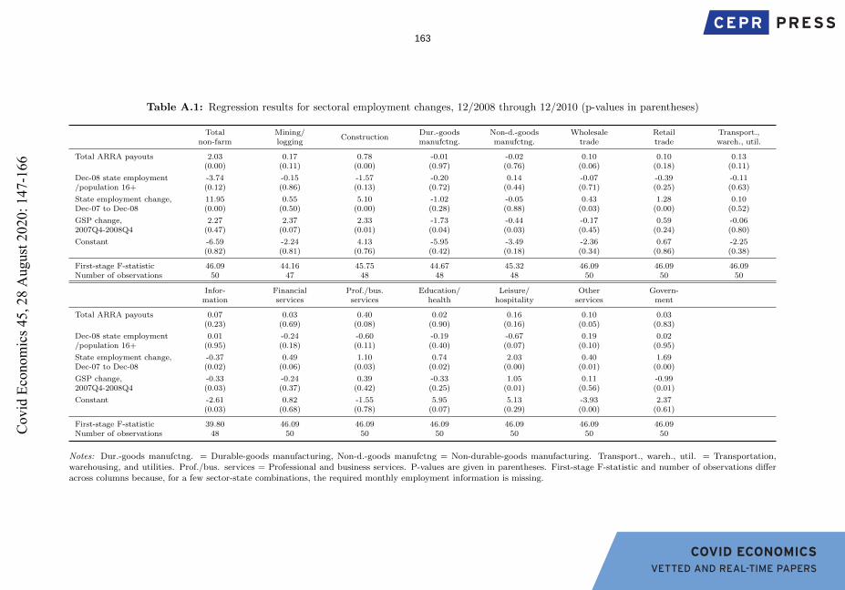
Table A.1 shows the full results of our baseline 2SLS regressions, which we use to estimate sector-

specific job-year coefficients as displayed in the pie chart in Figure 1. Each column corresponds to

a sector-specific regression.

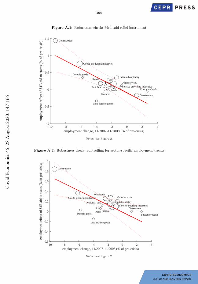
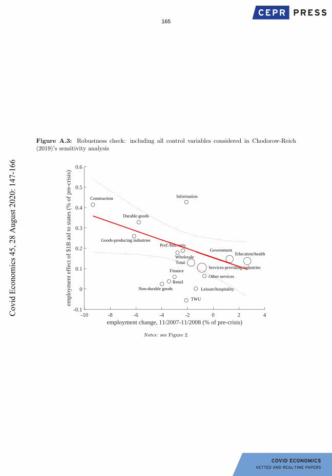
Figures A.1 through A.3 show the results of robustness checks. In Figure A.1, we used the

Medicaid relief instrument suggested by Chodorow-Reich et al. (2012) rather than the baseline

combination of instruments. In Figure A.2, we controlled for sector-specific pre-ARRA employment

trends. In Figure A.3, we accounted for the full set of control variables considered in Chodorow-

Reich (2019)’s sensitivity analysis. In all specifications, we find that sectors hit harder by the

recession were more strongly affected by state fiscal relief, as in our baseline specification.

Table A.2 shows the full results of the augmented sector-specific 2SLS regressions with inter-

action terms, given by

H∑h=0

(Ys,i,t+h − Ys,i,t) = αi + βiFs + ξiFsEi,s + ωiEi,s + γ′iXs + εs,i,

where

Ei,s =Ei,s −mean(Ei,s|i)

var(Ei,s|i)1/2

with

Ei,s =Employments,i,t−1 − Employments,i,t−13

Employments,i,t−13−

Employments,t−1 − Employments,t−13Employments,t−13

.

Each column of Table A.2 corresponds to a sector-specific regression.

162C

ovid

Eco

nom

ics 4

5, 2

8 A

ugus

t 202

0: 1

47-1

66


Table A.1: Regression results for sectoral employment changes, 12/2008 through 12/2010 (p-values in parentheses)

Total Mining/Construction

Dur.-goods Non-d.-goods Wholesale Retail Transport.,non-farm logging manufctng. manufctng. trade trade wareh., util.

Total ARRA payouts 2.03 0.17 0.78 -0.01 -0.02 0.10 0.10 0.13(0.00) (0.11) (0.00) (0.97) (0.76) (0.06) (0.18) (0.11)

Dec-08 state employment -3.74 -0.15 -1.57 -0.20 0.14 -0.07 -0.39 -0.11/population 16+ (0.12) (0.86) (0.13) (0.72) (0.44) (0.71) (0.25) (0.63)

State employment change, 11.95 0.55 5.10 -1.02 -0.05 0.43 1.28 0.10Dec-07 to Dec-08 (0.00) (0.50) (0.00) (0.28) (0.88) (0.03) (0.00) (0.52)

GSP change, 2.27 2.37 2.33 -1.73 -0.44 -0.17 0.59 -0.062007Q4-2008Q4 (0.47) (0.07) (0.01) (0.04) (0.03) (0.45) (0.24) (0.80)

Constant -6.59 -2.24 4.13 -5.95 -3.49 -2.36 0.67 -2.25(0.82) (0.81) (0.76) (0.42) (0.18) (0.34) (0.86) (0.38)

First-stage F-statistic 46.09 44.16 45.75 44.67 45.32 46.09 46.09 46.09Number of observations 50 47 48 48 48 50 50 50

Infor- Financial Prof./bus. Education/ Leisure/ Other Govern-mation services services health hospitality services ment

Total ARRA payouts 0.07 0.03 0.40 0.02 0.16 0.10 0.03(0.23) (0.69) (0.08) (0.90) (0.16) (0.05) (0.83)

Dec-08 state employment 0.01 -0.24 -0.60 -0.19 -0.67 0.19 0.02/population 16+ (0.95) (0.18) (0.11) (0.40) (0.07) (0.10) (0.95)

State employment change, -0.37 0.49 1.10 0.74 2.03 0.40 1.69Dec-07 to Dec-08 (0.02) (0.06) (0.03) (0.02) (0.00) (0.01) (0.00)

GSP change, -0.33 -0.24 0.39 -0.33 1.05 0.11 -0.992007Q4-2008Q4 (0.03) (0.37) (0.42) (0.25) (0.01) (0.56) (0.01)

Constant -2.61 0.82 -1.55 5.95 5.13 -3.93 2.37(0.03) (0.68) (0.78) (0.07) (0.29) (0.00) (0.61)

First-stage F-statistic 39.80 46.09 46.09 46.09 46.09 46.09 46.09Number of observations 48 50 50 50 50 50 50

Notes: Dur.-goods manufctng. = Durable-goods manufacturing, Non-d.-goods manufctng = Non-durable-goods manufacturing. Transport., wareh., util. = Transportation,warehousing, and utilities. Prof./bus. services = Professional and business services. P-values are given in parentheses. First-stage F-statistic and number of observations differacross columns because, for a few sector-state combinations, the required monthly employment information is missing.

163C

ovid

Eco

nom

ics 4

5, 2

8 A

ugus

t 202

0: 1

47-1

66


Figure A.1: Robustness check: Medicaid relief instrument

-10 -8 -6 -4 -2 0 2 4


-1

-0.5

0

0.5

1

1.5em

plo

ym

ent

effe

ct o

f $

1B

aid

to

sta

tes

(% o

f p

re-c

risi

s) Construction

Durable goods

Non-durable goods

Wholesale

Retail

TWU

Info

Finance

Prof./bus. serv.Education/health

Leisure/hospitality

Other services

Government

Total



Notes: see Figure 2.

Figure A.2: Robustness check: controlling for sector-specific employment trends

-10 -8 -6 -4 -2 0 2 4


-0.6

-0.4

-0.2

0

0.2

0.4

0.6

0.8

1

emplo

ym

ent

effe

ct o

f $1B

aid

to s

tate

s (%

of

pre

-cri

sis)

Leisure/hospitality


Prof./bus. serv.

TotalFinance

Construction

Wholesale

Info


Durable goods

Non-durable goods

Retail

TWU

Education/health

Other services

Government


164C

ovid

Eco

nom

ics 4

5, 2

8 A

ugus

t 202

0: 1

47-1

66


Figure A.3: Robustness check: including all control variables considered in Chodorow-Reich(2019)’s sensitivity analysis

-10 -8 -6 -4 -2 0 2 4


-0.1

0

0.1

0.2

0.3

0.4

0.5

0.6

emplo

ym

ent

effe

ct o

f $1B

aid

to s

tate

s (%

of

pre

-cri

sis)

Prof./bus. serv.

Services-providing industriesTotal

Other services

Leisure/hospitality

Durable goods

Construction

Non-durable goods

Wholesale

Retail

TWU

Information

Finance

Education/healthGovernment



165C

ovid

Eco

nom

ics 4

5, 2

8 A

ugus

t 202

0: 1

47-1

66


Table A.2: Regression results for sectoral employment changes, 12/2008 through 12/2010, interaction-term specification (p-values in parentheses)

ConstructionDur.-goods Non-d.-goods Wholesale Retail Transport., Infor-manufctng. manufctng. trade trade wareh., util. mation

Total ARRA payouts 0.88 0.03 -0.03 0.10 0.11 0.15 0.04(0.00) (0.90) (0.76) (0.09) (0.18) (0.08) (0.35)

Total ARRA payouts -0.15 -0.48 -0.04 -0.03 0.00 -0.04 -0.07× sector’s excess exposure (0.77) (0.32) (0.45) (0.48) (0.99) (0.81) (0.38)

Sector’s excess exposure 2.83 7.09 0.72 0.52 -0.06 0.55 1.05(0.64) (0.26) (0.33) (0.39) (0.97) (0.81) (0.33)

Dec-08 state employment+ -1.21 -0.53 0.07 -0.12 -0.38 -0.09 0.05/population 16+ (0.39) (0.38) (0.71) (0.54) (0.24) (0.69) (0.62)

State employment change, 4.11 -1.01 0.01 0.46 1.27 0.09 -0.28Dec-07 to Dec-08 (0.17) (0.28) (0.99) (0.02) (0.00) (0.55) (0.02)

GSP change, 2.20 -1.92 -0.43 -0.18 0.61 -0.06 -0.252007Q4-2008Q4 (0.03) (0.03) (0.04) (0.48) (0.22) (0.80) (0.02)

Constant -2.36 -2.58 -2.63 -1.84 0.48 -2.66 -2.62(0.90) (0.75) (0.37) (0.47) (0.90) (0.28) (0.04)

Number of observations 48 48 48 50 50 50 48

Financial Prof./bus. Education/ Leisure/ Other Govern-services services health hospitality services ment

Total ARRA payouts 0.01 0.32 -0.03 0.16 0.08 0.07(0.94) (0.20) (0.81) (0.09) (0.19) (0.79)

Total ARRA payouts -0.06 -0.12 -0.38 0.02 0.01 0.08× sector’s excess exposure (0.33) (0.26) (0.02) (0.85) (0.93) (0.79)

Sector’s excess exposure 1.14 2.80 6.27 0.18 0.01 -1.04(0.13) (0.09) (0.00) (0.91) (1.00) (0.76)

Dec-08 state employment -0.28 -0.48 -0.51 -0.54 0.17 0.04/population 16+ (0.07) (0.21) (0.02) (0.13) (0.16) (0.91)

State employment change, 0.55 0.50 1.87 1.98 0.47 1.64Dec-07 to Dec-08 (0.02) (0.29) (0.00) (0.00) (0.00) (0.02)

GSP change, -0.25 0.43 -0.21 0.91 0.14 -1.022007Q4-2008Q4 (0.37) (0.35) (0.48) (0.02) (0.42) (0.01)

Constant 1.64 -2.49 11.36 3.66 -3.47 1.65(0.38) (0.65) (0.00) (0.43) (0.05) (0.75)

Number of observations 50 50 50 50 50 50

Notes: Dur.-goods manufctng. = Durable-goods manufacturing, Non-d.-goods manufctng = Non-durable-goods manufacturing. Transport., wareh., util. = Transportation,warehousing, and utilities. Prof./bus. services = Professional and business services. P-values are given in parentheses. Number of observations differ across columns because, fora few sector-state combinations, the required monthly employment information is missing.

166C

ovid

Eco

nom

ics 4

5, 2

8 A

ugus

t 202

0: 1

47-1

66

covid economics - uni-wuppertal.de

Documents