coverage and capacity analysis of mmwave cellular systems

Coverage and Capacity Analysis of mmWave Cellular Systems

Robert W. Heath Jr. The University of Texas at Austin

Joint work with Tianyang Bai

www.profheath.org

http://www.profheath.org

http://www.profheath.org

WNCG Enhances UT Visibility Large multi-PI grants, e.g.

$1m Intel / Cisco grand challenge on video networks (PI: Heath) $1.3m on cross-layer delay-tolerant nets (PI: Shakkottai)

Seven major best paper awards in last four yearsWNCG Impacts Industry Definitive textbooks on wireless

Widely-cited magazine articles on hot topics

Developed key features of wireless standards

Software packages and toolkits

Host popular annual conference. www.twsummit.com

WNCG: Premier Wireless Research Center

1

WNCG AffiliatesWN

CG

Fac

ulty

20 faculty from 4 departments, all actively involved in center activities

Recent additions:

WN

CG

Stu

dent

s 120 PhD students in pooled space Many co-advised students 64%/yr intern at affiliates in last 4 yrs

• Students receive perks, special awards and travel funds for help with affiliates• Staff, space & other resources shared efficiently amongst all faculty/students

Affiliates champion large federal proposals, provide technical input/feedback, unrestricted gift funds

WNCG provides pre-prints, pre-competitive research ideas, vast expertise, first access to students

Wireless Networking andCommunica:ons Group

2

Andrea AlùMetamaterials

Joydeep GhoshData mining

François Baccelli *Stochasticgeometry

Alex Dimakis *Info theory

* New faculty at UT

http://www.twsummit.com/

http://www.twsummit.com/

Wireless Communications LabUndergrad/grad lab course

QAM & OFDM experiments

Complete lab manual & software

Uses USRP equipment

LabVIEW programming

Complete lab manual available

3

Dr. Robert W. Heath, University of Texas at Austin

DIGITAL COMMUNICATIONS

PHYSICAL LAYER EXPLORATION LAB USING THE NI USRP™ PLATFORM

front.pdf 1 9/12/11 4:46 PM

http://sine.ni.com/nips/cds/view/p/lang/en/nid/210087



Conclusions

mmWave isGreat for Cellular

There are many theoretical challenges

Introduction

(c) Robert W. Heath Jr. 2013

Why mmWave for Cellular?

Microwave

3 GHz 300 GHz

7

28 GHz 38-49 GHz 70-90 GHz300 MHz

Huge amount of spectrum available in mmWave bands*Cellular systems live with limited microwave spectrum ~ 600MHz

29GHz possibly available in 23GHz, LMDS, 38, 40, 46, 47, 49, and E-band

Technology advances make mmWave possibleSilicon-based technology enables low-cost highly-packed mmWave RFIC**

Commercial products already available (or soon) for PAN and LAN

Already deployed for backhaul in commercial products

1G-4G cellular 5G cellular

m i l l i m e t e r w a v e

* Z. Pi,, and F. Khan. "An introduction to millimeter-wave mobile broadband systems." IEEE Communications Magazine, vol. 49, no. 6, pp.101-107, Jun. 2011.** T.S. Rappaport, J. N. Murdock, and F. Gutierrez. "State of the art in 60-GHz integrated circuits and systems for wireless communications." Proceedings of the IEEE, vol. 99, no. 8, pp:1390-1436, 2011


Smaller wavelength means smaller captured energy at antenna3GHz->30GHz gives 20dB extra path loss due to aperture

Larger bandwidth means higher noise power and lower SNR50MHz -> 500MHz bandwidth gives 10dB extra noise power

The Need for Gain

8

Solution: Exploit array gain from large antenna arrays

microwave noise bandwidth

mmWave noise bandwidth

microwave aperture

mmWave aperture

TXRX

1

Summary of Cellular Millimeter Wave Channels

I. MEASUREMENT RESULTS

Aeff =�2

4⇡

Pr = D

✓�

4⇡R

◆2

Pr = AeffPt

4⇡R2

=

✓�

4⇡R

◆2

D =Pmax

(✓,�)

Pavg

1



Aeff =�2

4⇡

Pr = D

✓�

4⇡R

◆2

Pr = AeffPt

4⇡R2

=

✓�

4⇡R

◆2

D =Pmax

(✓,�)

Pavg


Antenna Arrays are Important

9

Narrow beams are a new feature of mmWaveReduces fading, multi-path, and interference

Implemented in analog due to hardware constraints

Baseband Processing

~100 antennas

Baseband Processing

antennas are small (mm)

highly directional MIMO transmission

used at TX and RX

Arrays will change system design principles


Traditional Beamforming Limitations

Power consumption limits the # of RF & ADC/DACs

Analog beamforming has additional constraintsConstant gains: Only phases is typically adjusted

Quantized phases: Fixed set of steering directions are allowed

10

Possible solution Precoding in the analog domain

RF

Phase shifters

Need beamforming strategies suitable for mmWave hardware

BasebandRF

Baseband

Hybrid Beamforming for mmWave

Combine both digital and analog beamforming

Small number of digital basebands (2 or 4)

Allows more advanced MIMO strategies to be exploited

Spatial multiplexing or multiuser MIMO

11

RF Chain

RF Chain

DigitalPrecoder

FBB

NBS

NMSN

RFN

S

RFChain

RF Chain

DigitalPrecoder

FBB

FRFFRF

Digital/Baseband

Analog/RF

NS

NRFBS

BS BSMS

Digital/Baseband

Analog/RF

RF Chain

RF Chain

DigitalPrecoder

FBB

NBS

NMSN

RFN

S

RFChain

RF Chain

DigitalPrecoder

FBB

FRFFRF

Digital/Baseband

Analog/RF

NS

NRFBS

BS BSMS

Digital/Baseband

Analog/RF

O. El Ayach, S. Abu-Surra, S. Rajagopal, Z. Pi, and R. W. Heath, Jr., `` Spatially Sparse Precoding in Millimeter Wave MIMO Systems,'' submitted to IEEE Trans. on Wireless, May 2013. Available on ArXiv.

Hybrid approach allows more advanced beam design

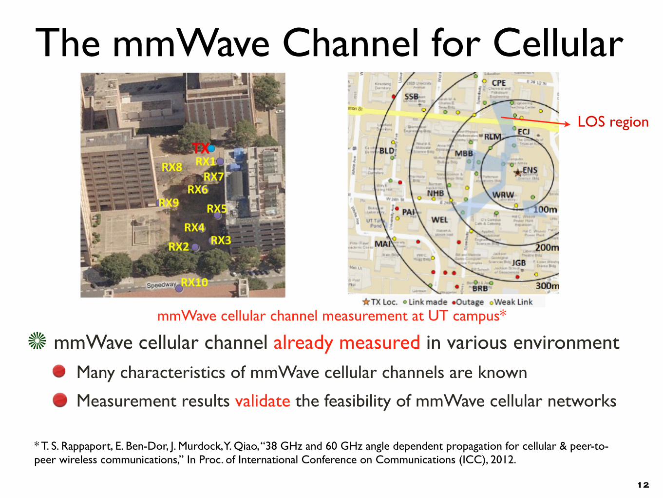
The mmWave Channel for Cellular

mmWave cellular channel already measured in various environmentMany characteristics of mmWave cellular channels are known

Measurement results validate the feasibility of mmWave cellular networks

12

38 GHz measurements between buildings were conducted in LOS, partially obstructed LOS, and NLOS links in clear weather, rain, and in hail storms. Worst-case attenuation of 26 dB above free space was found during a severe hail storm [1]. Narrowband millimeter wave propagation during weather events was studied in [13] where the Laws-Parsons model was shown to give reasonable statistical results of measured attenuation versus rain rate at 60 GHz, and showed the importance of the rain drop diameter.

In [14], a 230 m link at 35 GHz was studied and found excess attenuation of at least 2.5 dB for all rain events, and an excess attenuation of 10 dB or more occurring for 30% of the time.

II. MEASUREMENT HARDWARE The channel sounder used here employs a variable rate

PN sequence generator, adjusted to 400 Mcps for 38 GHz measurements and 750 Mcps for 60 GHz. The system is a superheterodyne with IF frequency of 5.4 GHz, which is fed to the millimeter wave up- and down-converters. The 38 and 60 GHz switchable up and down converters were built by Hughes Research Laboratories (HRL), and contain a mixer and LO frequency multipliers to yield carrier frequencies of 37.625 and 59.4 GHz. The 37.625 GHz carrier is sent at a power of 22 dBm and the 59.4 GHz carrier is sent at a power of 5 dBm. Since a sliding correlator requires a slower rate identical PN sequence, chip rates of 749.9625 MHz (slide factor of 20,000) and 399.95 MHz (slide factor of 8,000) were used for the 60 and 38 GHz receivers, respectively, to provide good processing gain and minimal pulse distortion. The system is able to measure at least 150dB of path loss in each band.

For 38 GHz, identical Ka-band vertically polarized horn antennas with gains of 25 dBi and half-power beamwidth of 7.0o were used at the transmitter and receiver. The 60 GHz peer-to-peer measurements used identical U-band vertically polarized horn antennas with gains of 25 dBi and beamwidth of 7.3o at the transmitter and receiver. All antennas were rotated on 3-D tripods.

III. EXPERIMENTAL DESIGN

A. Peer-to-Peer ChannelMeaurements For the peer-to-peer study, a single transmitter and ten

random receiver locations were chosen around a pedestrian walkway area surrounded by buildings of 1 to 12 stories. The

transmitter was placed 20 meters away from a 7 story building. The receiver was moved to locations with distances of 19 to 129 meters from the transmitter. The locations in Fig. 1 offered typical urban reflectors and scatterers such as automobiles, foliage, brick and aluminum-sided buildings, lampposts, signs, and handrails.

In order to characterize the various LOS and NLOS links present at each receiver location, the narrowbeam horn antennas were systematically steered in the azimuth direction

(similar to a beam-steering antenna array). For LOS links, the transmitter and receiver were first pointed directly at each other, corresponding to azimuth scanning angles of 0o for both the transmitter and receiver. Next, the transmitter antenna was pointed at the direction of a large scatterer. Then, the receiver antenna was steered to point towards that same scatterer. If a link was successfully established, a measurement was recorded. Next, the transmitter orientation was left fixed on the scatterer and the receiver antenna was then steered a full 360o to find and measure any additional links due to double-scattering or other propagation events. These additional links were found at most receiver locations, with one or two additional receiver angles at 60 GHz, and one to three different receiver angles at 38 GHz, although at substantially lower (-20 dB typ.) signal strength. All peer-to-peer receiver locations had a LOS path to the transmitter and, as a consequence, no outages were found for the peer-to-peer measurements.

Measurements made at each receiver location for a particular transmitter-receiver angle combination consisted of the average of eight local area point PDP measurements, where each point in the local-area was spaced equally on a circular measurement track with 10λ separation between each point. Each point PDP measurement consisted of a time average of 20 power delay profiles (PDPs) acquired in rapid succession over a fraction of second. As the receiver antenna was moved around the local area circular track, it was oriented to always point at the cause of the multipath link, as illustrated in Fig. 3. The eight local area PDPs were averaged together to form a local average PDP at each location. Fig. 4 shows a scatter plot of the receiver and transmitter azimuth angles that resulted in successful links. The plot shows a concentration in the second and fourth quadrants. On the right side of Fig. 4, both antennas are pointed at or near the same reflector. The

Figure 1. Overhead image of 38 and 60 GHz peer-to-peer measurement area with transmitter location marked as TX and receiver locations as RX#.

Figure 2. Overhead image of the outdoor cellular measurement area with the transmitter on a 5-story rooftop and receiver located on the ground.

6085

mmWave cellular channel measurement at UT campus*

* T. S. Rappaport, E. Ben-Dor, J. Murdock, Y. Qiao, “38 GHz and 60 GHz angle dependent propagation for cellular & peer-to-peer wireless communications,” In Proc. of International Conference on Communications (ICC), 2012.

Tx and Rx beams matching. We can see that radio propagation characteristics can be made more favorable by matching the best Tx and Rx beams.

FIGURE 2

Left : Measurement sites in UT Austin campus, Right : Pathloss and RMS delay spread results

Campaign 2: Dense Urban (New York, Manhattan), 28 GHz [14][15]

The second measurements were carried out at 28 GHz bands in Manhattan area. Channel bandwidth is 400 MHz, transmission power at amplifier 30 dBm, and horn antenna gain 24.5 dBi for both transmitter and receiver. Since these measurement environments are dense urban whose buildings have bricks and concrete walls, received signals are lower than at UT Austin campus. In these measurements, pathloss exponents are 1.68 in LOS and 4.58 in NLOS links, for the case of the best Tx and Rx beams matching.

AWG-14/INP-60

Page 5 of 8

LOS region

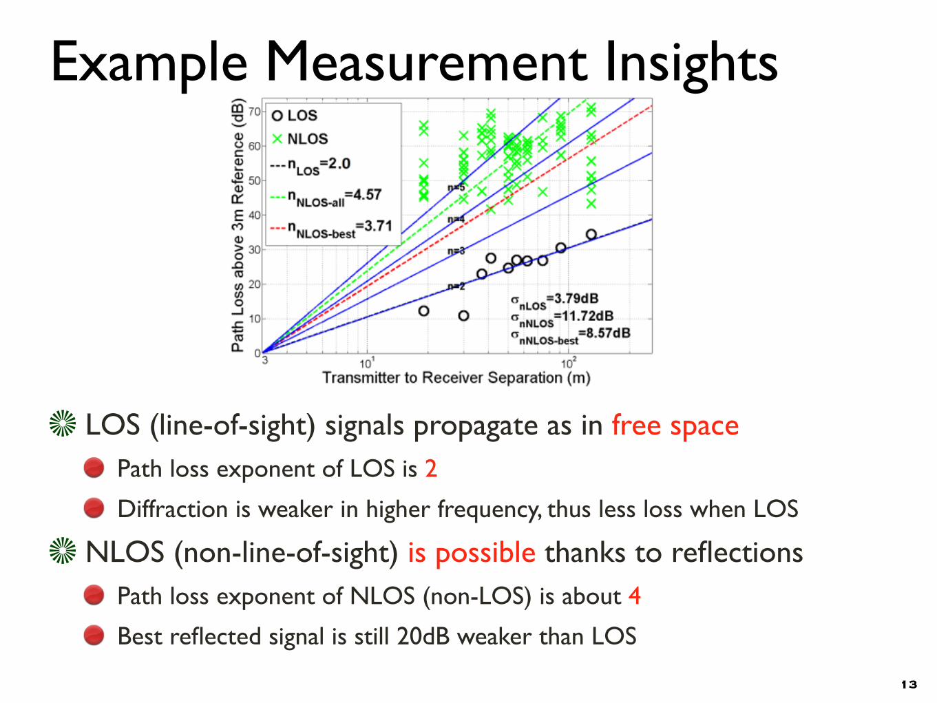
Example Measurement Insights

LOS (line-of-sight) signals propagate as in free spacePath loss exponent of LOS is 2

Diffraction is weaker in higher frequency, thus less loss when LOS

NLOS (non-line-of-sight) is possible thanks to reflectionsPath loss exponent of NLOS (non-LOS) is about 4

Best reflected signal is still 20dB weaker than LOS

13

Figure 6. Scatter plot of the measured path loss values relative to 3 m free space path loss for the 60 GHz outdoor urban peer-to-peer channel.

Figure 7. Scatter plot of the measured path loss values relative to 3 m free space path loss for the 38 GHz outdoor urban peer-to-peer channel.

exponents for all LOS links, all NLOS links, and for the strongest (best) NLOS link selected from all unique antenna pointing combinations for each receiver location. All path loss measurements were based on a common free space close-in anchor/reference distance of 3 meters at which the free space reference path loss is 77.5 and 73.5 dB for 60 and 38 GHz, respectively. The 60 GHz LOS links have a path loss exponent of 2.25, slightly greater than free space and a standard deviation of 2 dB. The LOS path loss exponent being slightly greater than 2 is due to atmospheric absorption of 60 GHz [15]. For millimeter wave systems using beam-steering antenna arrays, once the LOS path is completely blocked, the beam will be steered until the strongest NLOS link is identified. Thus, we considered the strongest NLOS link that can be made at each location, as this link is the one which future systems will need to select. Figs. 6 and 7 indicate advantages for systems that can find the strongest NLOS link over those which receive a random NLOS link. Fig. 6 shows the strongest 60 GHz NLOS links have a path loss exponent of 3.76, as compared to 4.22 when all possible NLOS links are considered. The stronger NLOS links were also characterized by lower RMS delay spreads.

Fig. 7 shows a path loss scatter plot for the 38 GHz peer-to-peer channel, which exhibited free space LOS propagation (n=2). Interestingly, NLOS links for the 38 GHz channel had a greater path loss exponent of 4.57 than 60 GHz peer-to-peer NLOS links when all NLOS links were considered, but a slightly better path loss exponent of 3.71 when considering only the strongest NLOS links at each location. Comparing Figs. 4, 6 and 7, we can infer differences in specular scattering at 38 versus 60 GHz. The longer wavelength of 38 GHz results in rough surfaces appearing more smooth, so that the same environment will provide more links created through scattering off rough surfaces at 38 GHz, and with less free space loss than at 60 GHz. Therefore, at 38 GHz, many more

links (some very weak) are made as compared to 60 GHz. When the best path is selected, we see the path loss for identical beamwidth antennas in 38 GHz and 60 GHz NLOS channels are similar (n=3.71 @ 38GHz vs. 3.76 @ 60GHz).

Fig. 8 shows the cumulative distribution function (CDF) of the RMS delay spreads measured for the peer-to-peer channel at both 38 and 60 GHz. From the plot, it is apparent that LOS links do not show any resolvable multipath, with differences between 60 GHz and 38 GHz links attributable to the difference in the chip rates. Notably, the 38 GHz channel was characterized by higher RMS delay spreads compared to the 60 GHz channel, with mean RMS delay spreads of 23.6 ns and 7.4 ns for the 38 and 60 GHz channels, respectively. This is likely due to lower free space path loss and more objects in the environment serving as scatterers at 38 GHz than at 60 GHz. The plot shows the expected and maximum values for the RMS delay spread.

Figure 8. CDF of the RMS delay spread for the 38 and 60 GHz urban outdoor peer-to-peer channels.

Figure 9. Larger absolute azimuth pointing angles at the receiver, transmitter, or both are associated with probabilistically higher RMS delay spreads. Fit lines are added to illustrate the increased mean RMS delay spread.

Fig. 9 shows a scatter plot of measured RMS delay spread vs. the sum of the absolute values for the azimuth pointing angles of the transmitter and receiver antennas for each link over all locations. The plot reveals that large scanning angles at the transmitter or receiver (or both) exhibit high RMS delay spread paths more often than narrow scanning angle paths. This is likely due to the greater travel distance of NLOS links formed with large or extreme azimuth pointing angles (greater than 500), and hence the larger number of objects illuminated by the transmitter for these links. This is an important trend for beam-steering algorithm development, as wide scan-angle links will require greater channel equalization as well as longer propagation time than shorter LOS links.

6087


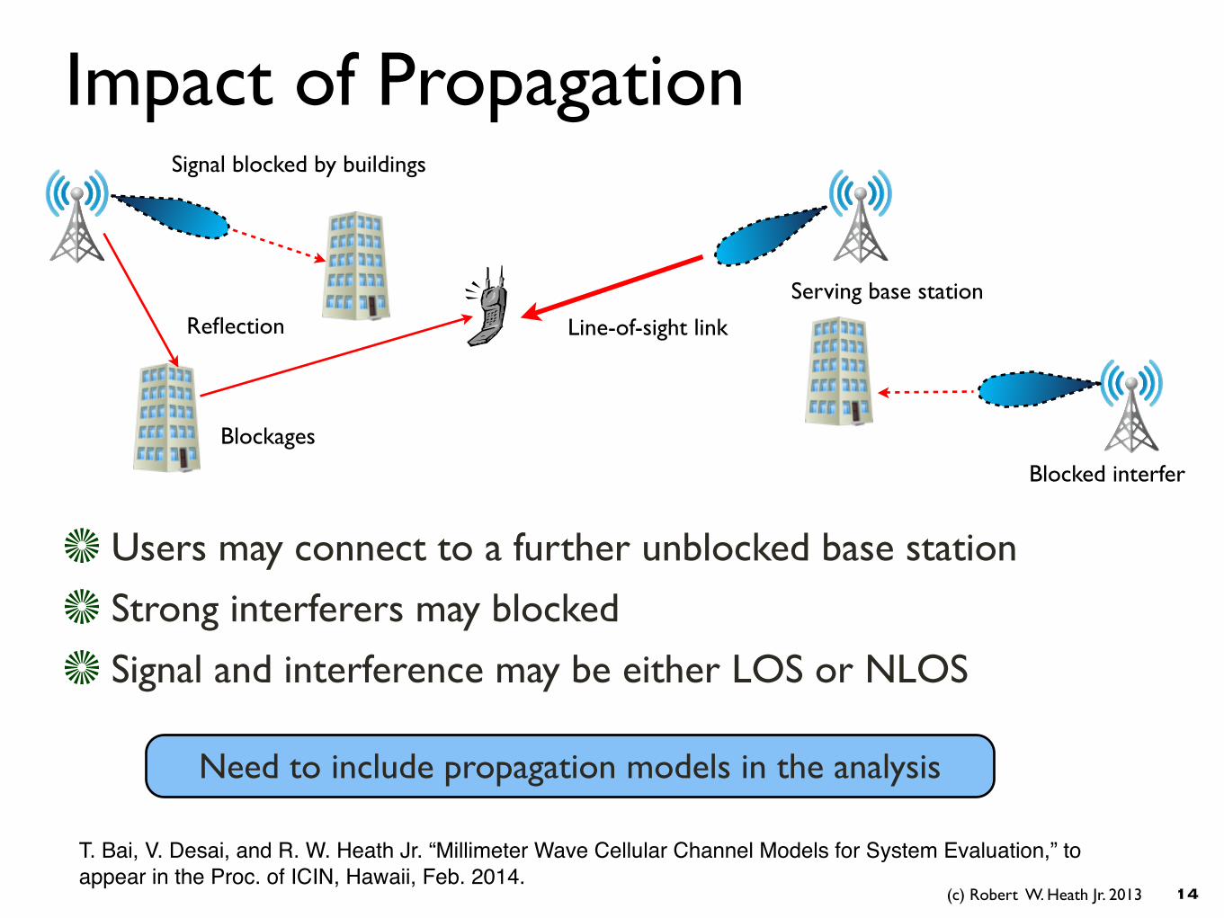
Impact of Propagation

Users may connect to a further unblocked base station

Strong interferers may blocked

Signal and interference may be either LOS or NLOS

14

Need to include propagation models in the analysis

T. Bai, V. Desai, and R. W. Heath Jr. “Millimeter Wave Cellular Channel Models for System Evaluation,” to appear in the Proc. of ICIN, Hawaii, Feb. 2014.

Line-of-sight linkReflection

Blockages

Signal blocked by buildings

Serving base station

Blocked interfer


mmWave Performance Analysis

15

LOS & non-LOS linksDirectional Beamforming (BF)

How to including beamforming + blockages in mmWave cellular analysis?

Need to incorporate directional beamformingRX and TX communicate via main lobes to achieve array gain

Steering directions at interfering BSs are random

Need to distinguish LOS and NLOS pathsIncorporate different characteristics in LOS & NLOS channels

Better characterize blockages

Stochastic Geometry for mmWave Cellular

System Analysis


Stochastic Geometry for Cellular

Stochastic geometry is a tool for analyzing microwave cellularReasonable fit with real deployments

Closed form solutions for coverage probability available

Provides a system-wide performance characterization

17

J. G. Andrews, F. Baccelli, and R. K. Ganti, "A Tractable Approach to Coverage and Rate in Cellular Networks", IEEE Transactions on Communications, November 2011.T. X. Brown, "Cellular performance bounds via shotgun cellular systems," IEEE JSAC, vol.18, no.11, pp.2443,2455, Nov. 2000.

base station locations distributed (usually) as a

Poisson point process (PPP)performance analyzed for a typical user

Need to incorporate LOS/non-LOS links and directional antennas

Baccelli


Poisson Point Processes

Poisson point process (PPP): the simplest point process# of points is a Poisson variable with mean λS

Given N points in certain area, locations independent

Useful results like Campbell’s Theorem & Displacement Theorem apply

Assigning each point an i.i.d. random variable forms a marked PPP

18

14

Fig. 7. .

Antenna steering orientations as marks of the

BS PPP


Blockages in mmWave

Use random shape theory to model buildingsModel random buildings as a rectangular Boolean scheme

Buildings distributed as PPP with independent sizes & orientations

Compute the LOS probability based on the building model# of blockages on a link is a Poisson random variable

The LOS probability that no blockage on a link of length R is

19

Boolean scheme of rectanglesK: # of blockages on a link

Randomly located buildings

e��R

LOS: K=0non-LOS

K>0

Tianyang Bai and R. W. Heath, Jr., ``Using Random Shape Theory to Model Blockage in Random Cellular Networks,'' Proc. of the International Conf. on Signal Processing and Communications, Bangalore, India, July 22-25, 2012.


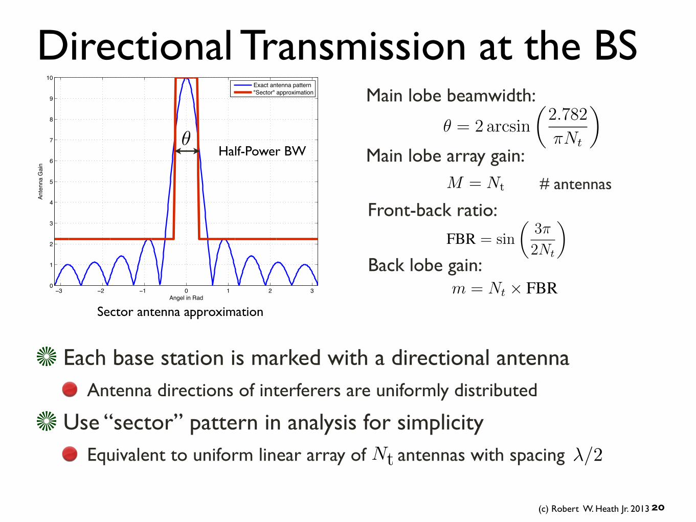
Directional Transmission at the BS

Each base station is marked with a directional antennaAntenna directions of interferers are uniformly distributed

Use “sector” pattern in analysis for simplicityEquivalent to uniform linear array of antennas with spacing

20

1



−3 −2 −1 0 1 2 30

1

2

3

4

5

6

7

8

9

10

Angel in Rad

Ante

nna

Gai

n

Exact antenna pattern"Sector" approximation

Fig. 1.

Sector antenna approximation

Half-Power BW✓

Nt �/2

Main lobe beamwidth:

Main lobe array gain:M = Nt

Front-back ratio:

Back lobe gain:

3

✓ = 2arcsin

✓2.782

⇡Nt

◆

FBR = sin

✓3⇡

2Nt

◆

m = Nt ⇥ FBR

3

✓ = 2arcsin

✓2.782

⇡Nt

◆

FBR = sin

✓3⇡

2Nt

◆

m = Nt ⇥ FBR

3

✓ = 2arcsin

✓2.782

⇡Nt

◆

FBR = sin

✓3⇡

2Nt

◆

m = Nt ⇥ FBR

# antennas


15

Fig. 8. .

Proposed mmWave Model

Use stochastic geometry to model BSs as marked PPPModel the steering directions as independent marks of the BSs

Use random shape theory to model buildingsModel the building as rectangle Boolean schemes

Different path loss exponents for LOS and non-LOS paths

21

PPP Interfering BSs

Serving BS

Buildings

Typical User

Reflections


System Parameters Different path loss model for LOS and nonLOS links

Line-of-sight with probability

LOS path Loss in dB:

Non-LOS path loss in dB:

28Ghz system: let C=50 dB, K=10 dB

General small scale fadingNo fading case: small scaling fading is minor in mmWave [RapSun]

Link budgetTx antenna input power: 30dBm

Signal bandwidth: 500 MHz (Noise: -87 dBm)

Noise figure: 5dB

22

e��R

PL2 = C +K + 40 logR(m)

PL1 = C + 20 logR(m)

h

Results on Coverage


Coverage Analysis

24

where

7

P(SINR > T ) =

Z 1

�1

Z 1

0

E[e�tP

k

Lk |L⇤

= x ]fL⇤(x)

e

j2⇡t/T � 1

j2⇡tdxdt,

E[e�tP

k

Lk |L⇤

= x ] = exp

� sx

MrMt⇢+

Z 1

x

⇣ptpre

� sx

u

+ (1� pt)pre� sxmt

uMt+ pt(1� pr)e

� sxmruMr

+(1� pt)(1� pr)e� sxmtmr

uMrMt � 1

⌘⇤(du)

i,

Li = r↵i

i ,

L⇤= max

i{Li} ,

SINR =

MrMtH0`(r0)

N0/Pt +P

k>0 AkBkHk`(rk),

`(x) =

8<

:Cx�2 w. p. e��x

C Kx�4 w. p. 1� e

��x,

Ak =

8<

:Mt w. p. ✓t

2⇡

mt w. p. 1� ✓t2⇡

,

Bk =

8<

:Mr w. p. ✓r

2⇡

mr w. p. 1� ✓r2⇡

,

H0`(r0) = min

k>0{Hk`(rk)} ,

7

P(SINR > T ) =

Z 1

�1

Z 1

0

E[e�tP

k

Lk |L⇤

= x ]fL⇤(x)

e

j2⇡t/T � 1

j2⇡tdxdt,

E[e�tP

k

Lk |L⇤

= x ] = exp

� sx

MrMt⇢+

Z 1

x

⇣ptpre

� sx

u


uMt+ pt(1� pr)e

� sxmruMr


uMrMt � 1

⌘⇤(du)

i,

Li = r↵i

i ,

L⇤= max

i{Li} ,

SINR =

MrMtH0`(r0)

N0/Pt +P

k>0 AkBkHk`(rk),

`(x) =

8<

:Cx�2 w. p. e��x

C Kx�4 w. p. 1� e

��x.

Ak =

8<

:Mt w. p. ✓t

2⇡

mt w. p. 1� ✓t2⇡

,

Bk =

8<

:Mr w. p. ✓r

2⇡

mr w. p. 1� ✓r2⇡

,

H0`(r0) = min

k>0{Hk`(rk)} ,

Connecting to the strongest signal before BF

Array gain of the TX antenna

Array gain of the RX antenna

Path Loss of LOS or non-LOS

Serving BS and User connect via main lobe

Use stochastic geometry to compute SINR distribution

General small-scale fading

7

P(SINR > T ) =

Z 1

�1

Z 1

0

E[e�tP

k

Lk |L⇤

= x ]fL⇤(x)

e

j2⇡t/T � 1

j2⇡tdxdt,

E[e�tP

k

Lk |L⇤

= x ] = exp

� sx

MrMt⇢+

Z 1

x

⇣ptpre

� sx

u


uMt+ pt(1� pr)e

� sxmruMr


uMrMt � 1

⌘⇤(du)

i,

Li = r↵i

i ,

L⇤= max

i{Li} ,

SINR =

NrNtH0`(r0)

N0/Pt +P

k>0 AkBkHk`(rk),

`(x) =

8<

:Cx�2 w. p. e��x

C Kx�4 w. p. 1� e

��x.

Ak =

8<

:Nt w. p. ✓t

2⇡

NtFBRt w. p. 1� ✓t2⇡

,

Bk =

8<

:Nr w. p. ✓r

2⇡

NrFBRr w. p. 1� ✓r2⇡

,

H0`(r0) = min

k>0{Hk`(rk)} ,

7

P(SINR > T ) =

Z 1

�1

Z 1

0

E[e�tP

k

Lk |L⇤

= x ]fL⇤(x)

e

j2⇡t/T � 1

j2⇡tdxdt,

E[e�tP

k

Lk |L⇤

= x ] = exp

� sx

MrMt⇢+

Z 1

x

⇣ptpre

� sx

u


uMt+ pt(1� pr)e

� sxmruMr


uMrMt � 1

⌘⇤(du)

i,

Li = r↵i

i ,

L⇤= max

i{Li} ,

SINR =

NrNtH0`(r0)

N0/Pt +P

k>0 AkBkHk`(rk),

`(x) =

8<

:Cx�2 w. p. e��x

C Kx�4 w. p. 1� e

��x.

Ak =

8<

:Nt w. p. ✓t

2⇡


,

Bk =

8<

:Nr w. p. ✓r

2⇡


,

H0`(r0) = min

k>0{Hk`(rk)} ,

7

P(SINR > T ) =

Z 1

�1

Z 1

0

E[e�tP

k

Lk |L⇤

= x ]fL⇤(x)

e

j2⇡t/T � 1

j2⇡tdxdt,

E[e�tP

k

Lk |L⇤

= x ] = exp

� sx

MrMt⇢+

Z 1

x

⇣ptpre

� sx

u


uMt+ pt(1� pr)e

� sxmruMr


uMrMt � 1

⌘⇤(du)

i,

Li = r↵i

i ,

L⇤= max

i{Li} ,

SINR =

NrNtH0`(r0)

N0/Pt +P

k>0 AkBkHk`(rk),

`(x) =

8<

:Cx�2 w. p. e��x

C Kx�4 w. p. 1� e

��x.

Ak =

8<

:Nt w. p. ✓t

2⇡


,

Bk =

8<

:Nr w. p. ✓r

2⇡


,

H0`(r0) = min

k>0{Hk`(rk)} ,


Coverage Probability of mmWaveMain Theorem [mmWave Coverage probability] The coverage probability can be computed as

where

,

,

.

25

P[SINR > T ]

4

P(SINR > T ) =

Z 1

�1

Z 1

0

U(x, t)fL⇤(x)

e

j2⇡t/T � 1

j2⇡tdxdt

U(x, s) = exp

� sx

MrMt⇢+

Z 1

x

⇣ptpre

� sx

u


uMt+ pt(1� pr)e

� sxmruMr


uMrMt � 1

⌘⇤(du)

i

⇤(x) = 2⇡�

0

@Z x

14

0

t�1� e

��t�dt+

Z px

0

te��tdt

1

A

⇤L(x) = 2⇡�

Z px

0

te��tdt

⇤NL(x) = 2⇡�

Z(

x

K

)

1/4

0

t�1� e

��t�dt

fL⇤(x) = � d

dxe

�⇤(x)

Li = r↵i

i

L⇤= max

i{Li}

F =

1

SINR

E⇥e

�sF |L⇤= x

⇤= U(x, s)

E⇥e

�sF⇤=

Z 1

0

U(x, s)fL⇤(x)dx

4

P(SINR > T ) =

Z 1

�1

Z 1

0

U(x, t)fL⇤(x)

e

j2⇡t/T � 1

j2⇡tdxdt

U(x, s) = exp

� sx

MrMt⇢+

Z 1

x

⇣ptpre

� sx

u


uMt+ pt(1� pr)e

� sxmruMr


uMrMt � 1

⌘⇤(du)

i

⇤(x) = 2⇡�

0

@Z x

14

0

t�1� e

��t�dt+

Z px

0

te��tdt

1

A

⇤L(x) = 2⇡�

Z px

0

te��tdt

⇤NL(x) = 2⇡�

Z(

x

K

)

1/4

0

t�1� e

��t�dt

fL⇤(x) = � d

dxe

�⇤(x)

Li = r↵i

i

L⇤= max

i{Li}

F =

1

SINR

E⇥e

�sF |L⇤= x

⇤= U(x, s)

E⇥e

�sF⇤=

Z 1

0

U(x, s)fL⇤(x)dx

4

P(SINR > T ) =

Z 1

�1

Z 1

0

U(x, t)fL⇤(x)

e

j2⇡t/T � 1

j2⇡tdxdt

U(x, s) = exp

� sx

MrMt⇢+

Z 1

x

⇣ptpre

� sx

u


uMt+ pt(1� pr)e

� sxmruMr


uMrMt � 1

⌘⇤(du)

i

⇤(x) = 2⇡�

0

@Z x

14

0

t�1� e

��t�dt+

Z px

0

te��tdt

1

A

⇤L(x) = 2⇡�

Z px

0

te��tdt

⇤NL(x) = 2⇡�

Z(

x

K

)

1/4

0

t�1� e

��t�dt

fL⇤(x) = � d

dxe

�⇤(x)

Li = r↵i

i

L⇤= max

i{Li}

F =

1

SINR

E⇥e

�sF |L⇤= x

⇤= U(x, s)

E⇥e

�sF⇤=

Z 1

0

U(x, s)fL⇤(x)dx

Transform interference field into 1D space by Displacement Thm

4

P(SINR > T ) =

Z 1

�1

Z 1

0

U(x, t)fL⇤(x)

e

j2⇡t/T � 1

j2⇡tdxdt

U(x, s) = exp

� sx

MrMt⇢+

Z 1

x

⇣ptpre

� sx

u


uMt+ pt(1� pr)e

� sxmruMr


uMrMt � 1

⌘⇤(du)

i

⇤(x) = 2⇡�Eh

"Z(

xh

K

)

0.25

0

t�1� e

��t�dt+

Z pxh

0

te��tdt

#

⇤L(x) = 2⇡�

Z px

0

te��tdt

⇤NL(x) = 2⇡�

Z(

x

K

)

1/4

0

t�1� e

��t�dt

fL⇤(x) = � d

dxe

�⇤(x)

Li = r↵i

i

L⇤= max

i{Li}

F =

1

SINR

E⇥e

�sF |L⇤= x

⇤= U(x, s)

E⇥e

�sF⇤=

Z 1

0

U(x, s)fL⇤(x)dx


10

−10 −8 −6 −4 −2 0 2 4 6 8 100.2

0.3

0.4

0.5

0.6

0.7

0.8

0.9

1

SINR Threshold

Co

ve

rag

e P

rob

ab

ilit

y

Nt=64, θ=1.6o

Nt=32, θ=3.2O

Nt=16, θ=6.5o

Microwave: SU MIMO 4X4

Fig. 6.

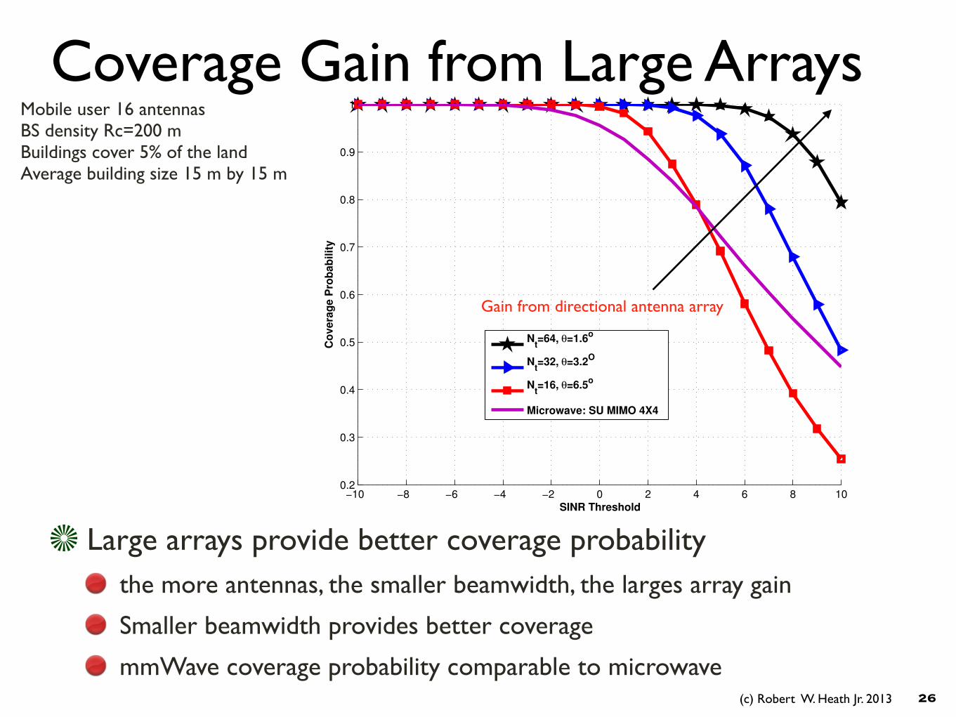
Coverage Gain from Large Arrays

26

Mobile user 16 antennasBS density Rc=200 mBuildings cover 5% of the landAverage building size 15 m by 15 m

Large arrays provide better coverage probabilitythe more antennas, the smaller beamwidth, the larges array gain

Smaller beamwidth provides better coverage

mmWave coverage probability comparable to microwave

Gain from directional antenna array


10

−10 −8 −6 −4 −2 0 2 4 6 8 10

0.4

0.5

0.6

0.7

0.8

0.9

1

SINR Threshold

Co

ve

rag

e P

rob

ab

ilit

y

rc=50 m

rc=100 m

rc=200 m

rc=300 m

Microwave: 4X4 SU MIMO

Fig. 6.

Coverage Gain from Higher Density

27

Higher density can also increase coverage probabilityCoverage probability no longer invariant with BS density

Become interference-limited when coverage probability is good

32 antennas at BSBlockages covers 10% land

Noise-limited region due to high path loss

Interference-limited region

Gain over microwave


LOS & non-LOS Path Loss

Coverage probability differs in LOS and non-LOS regionNeed to incorporate blockage model & differentiate LOS and nonLOS

Non-LOS coverage probability generally provides a lower bound

Buildings may improve coverage by blocking more interference28

7

−10 −8 −6 −4 −2 0 2 4 6 8 100.2

0.3

0.4

0.5

0.6

0.7

0.8

0.9

1

SINR Threshold

Co

ve

rag

e P

rob

ab

ilit

y

Proposed model

LOS path loss only

non−LOS path loss only

Fig. 2. .

32 antennas at BSsBlockages covers 10% landRc=100 m

Gain from blocking more interference

pure LOS (no buildings)

pure NLOS

proposed model


LOS & Reflection CoverageCorollary 1 [Coverage probability by LOS BSs]

The coverage probability provided by LOS BSs is

,

where

29

6

P(SINR > T ) =

Z 1

�1

Z 1

0

U1(x, t)U2(t)fL⇤(x)

e

j2⇡t/T � 1

j2⇡tdxdt

U2(s) = exp

Z 1

0

⇣ptpre

� sx

u


uMt+ pt(1� pr)e

� sxmruMr


uMrMt � 1

⌘⇤2(du)

i

U1(x, s) = exp

� sx

MrMt⇢+

Z 1

x

⇣ptpre

� sx

u


uMt+ pt(1� pr)e

� sxmruMr


uMrMt � 1

⌘⇤1(du)

i

⇤1(x) = 2⇡�

Z px

0

te��tdt

⇤2(x) = 2⇡�

Z(

x

K

)

1/4

0

t�1� e

��t�dt

fL⇤(x) = � d

dxe

�⇤1(x)

6

P(SINR > T ) =

Z 1

�1

Z 1

0


e

j2⇡t/T � 1

j2⇡tdxdt

U2(s) = exp

Z 1

0

⇣ptpre

� sx

u


uMt+ pt(1� pr)e

� sxmruMr


uMrMt � 1

⌘⇤2(du)

i,

U1(x, s) = exp

� sx

MrMt⇢+

Z 1

x

⇣ptpre

� sx

u


uMt+ pt(1� pr)e

� sxmruMr


uMrMt � 1

⌘⇤1(du)

i,

⇤1(x) = 2⇡�

Z px

0

te��tdt,

⇤2(x) = 2⇡�

Z(

x

K

)

1/4

0

t�1� e

��t�dt,

fL⇤(x) = � d

dxe

�⇤1(x).

6

P(SINR > T ) =

Z 1

�1

Z 1

0


e

j2⇡t/T � 1

j2⇡tdxdt

U2(s) = exp

Z 1

0

⇣ptpre

� sx

u


uMt+ pt(1� pr)e

� sxmruMr


uMrMt � 1

⌘⇤2(du)

i,

U1(x, s) = exp

� sx

MrMt⇢+

Z 1

x

⇣ptpre

� sx

u


uMt+ pt(1� pr)e

� sxmruMr


uMrMt � 1

⌘⇤1(du)

i,

⇤1(x) = 2⇡�

Z px

0

te��tdt,

⇤2(x) = 2⇡�

Z(

x

K

)

1/4

0

t�1� e

��t�dt,

fL⇤(x) = � d

dxe

�⇤1(x).

6

P(SINR > T ) =

Z 1

�1

Z 1

0


e

j2⇡t/T � 1

j2⇡tdxdt

U2(s) = exp

Z 1

0

⇣ptpre

� sx

u


uMt+ pt(1� pr)e

� sxmruMr


uMrMt � 1

⌘⇤2(du)

i,

U1(x, s) = exp

� sx

MrMt⇢+

Z 1

x

⇣ptpre

� sx

u


uMt+ pt(1� pr)e

� sxmruMr


uMrMt � 1

⌘⇤1(du)

i,

⇤1(x) = 2⇡�

Z px

0

te��tdt,

⇤2(x) = 2⇡�

Z(

x

K

)

1/4

0

t�1� e

��t�dt,

fL⇤(x) = � d

dxe

�⇤1(x).

6

P(SINR > T ) =

Z 1

�1

Z 1

0


e

j2⇡t/T � 1

j2⇡tdxdt

U2(s) = exp

Z 1

0

⇣ptpre

� sx

u


uMt+ pt(1� pr)e

� sxmruMr


uMrMt � 1

⌘⇤2(du)

i,

U1(x, s) = exp

� sx

MrMt⇢+

Z 1

x

⇣ptpre

� sx

u


uMt+ pt(1� pr)e

� sxmruMr


uMrMt � 1

⌘⇤1(du)

i,

⇤1(x) = 2⇡�

Z px

0

te��tdt,

⇤2(x) = 2⇡�

Z(

x

K

)

1/4

0

t�1� e

��t�dt,

fL⇤(x) = � d

dxe

�⇤1(x).

6

P(SINR > T ) =

Z 1

�1

Z 1

0


e

j2⇡t/T � 1

j2⇡tdxdt

U2(s) = exp

Z 1

0

⇣ptpre

� sx

u


uMt+ pt(1� pr)e

� sxmruMr


uMrMt � 1

⌘⇤2(du)

i,

U1(x, s) = exp

� sx

MrMt⇢+

Z 1

x

⇣ptpre

� sx

u


uMt+ pt(1� pr)e

� sxmruMr


uMrMt � 1

⌘⇤1(du)

i,

⇤1(x) = 2⇡�

Z px

0

te��tdt,

⇤2(x) = 2⇡�

Z(

x

K

)

1/4

0

t�1� e

��t�dt,

fL⇤(x) = � d

dxe

�⇤1(x).

Coverage probability by reflections derived in a similar way


10

−10 −8 −6 −4 −2 0 2 4 6 8 100

0.1

0.2

0.3

0.4

0.5

0.6

0.7

0.8

0.9

1

SINR Threshold

Co

ve

rag

e P

rob

ab

ilit

y

Overall coverage probability

Covergage probability by LOS BSs

Coverage probability by reflections

Fig. 6.

Reflections Improve Coverage

Reflections can establish links in the shadowed areasWith dense blockages, most users are served by reflected links

Non-LOS links improve the coverage probability of mmWave

30

128 antennas at BSsBlockages covers 30% land(Heavy shadowing case)Rc=200 m

With dense blockages, a large fraction of users is non-LOS

Results on Rate


Data Rate ComparisonGiven coverage probability, the achievable rate is

Microwave network 4X4 MU MIMO with bandwidth 50MHz: Spectrum efficiency is 4.95 bps/ Hz

Data rate is 248 Mbps (invariant with the cell size Rc)

mmWave network with bandwidth 500MHz:

32

3

A. Distribution of L0

Lemma 8: The probability density function (pdf) of L0 is fL0(x) = ⇤

0(x)(e)⇤x, where ⇤

0(x) =

d⇤(x)dx , ⇤(x) = ⇤1(x) + ⇤2(x), and

⇤1(x) = 2⇡�EH1

"Z pxH1

0

te��tdt

#, (3)

⇤2(x) = 2⇡�EH2

"Z pxH2

0

t�1� e

��t�dt

#. (4)

Remark 9: Note that if there is no fading in both LOS and non-LOS links, then

⇤1(x) = 2⇡�

Z px

0

te��tdt, (5)

⇤2(x) = 2⇡�

Z px

0

t�1� e

��t�dt. (6)

B. Laplace Transform of F

First, we compute the conditional Laplace transform of F, given that L0 = x, in the following

lemma.

Lemma 10: Given that L0 = x, the conditional Laplace transform of F is

E⇥e

�sF |L0 = x⇤= e

�sx

M⇢

exp

✓Z 1

x

⇣e

�Msx

u � 1

⌘ ✓

2⇡⇤(u)du

◆exp

✓Z 1

x

�e

�msx

u � 1

�2⇡ � ✓

2⇡⇤(u)du

◆

(7)The unconditional Laplace transform of F is

E⇥e

�sF⇤=

Z 1

0

E⇥e

�sF |L0 = x⇤fL0(x)dx (8)

C. Computation of Coverage probability

Using Parseval’s Theorem, we can obtain the coverage probability as

Pc(T ) = P(SINR > T ) (9)

= P(F < 1/T ) (10)

=

Z 1

0

E⇥e

�sF⇤e

j2⇡/T � 1

j2⇡dt (11)

D. Rate

As we did previously, the achievable rate ⌘ can be computed as

⌘ =

Z 1

0

Pc(T )

1 + TdT (12)

100m 200m

32 3.4Gbps 3.25Gbps

64 3.8Gbps 3.45Gbps

NtRc

mmWave achieves high gain in average rate

16 antenna at MSBlockages covers 10% land

# of antenna at BS

Average cell radius


7

0 500 1000 1500 2000 2500 3000 3500 4000 4500 50000

0.1

0.2

0.3

0.4

0.5

0.6

0.7

0.8

0.9

1

Cell Throughput in Mbps

Rate

Co

vera

ge P

rob

ab

ilit

y

CoMP: Nt=4, 2 Users, 3 BSs/ Cluster

Massive MIMO: Nt=∞

mmWave: Nt=64, R

c=100m

SU MIMO: 4X4

Fig. 3.

Cell Throughput Comparison

33

Gain from larger bandwidth

Gain from serving multiple users

mmWave can support much higher data rate

* for more information on this setup refer to: Robert W. Heath Jr., “ Role of MIMO Beyond LTE: Massive? Coordinated? mmWave?”, Workshop on Beyond 3GPP LTE-A ICC 2013.

Conclusions


Going Forward with mmWave

mmWave coverage probability and rateNeed to include both LOS and Non-LOS conditions

Interference is reduced by directional antennas and blockages

Good rates and coverage can be achieved

Theoretical challenges aboundAnalog beamforming algorithms & hybrid beamforming

Channel estimation, exploiting sparsity, incorporating robustness

Multi-user beamforming algorithms and analysis

Microwave-overlaid mmWave system a.k.a. phantom cells

More advanced stochastic geometry models including multi-tier

35


Questions?

36

T. Rappaport, R. W. Heath Jr., R. C. Daniels, and J. Murdock, Millimeter Wave Wireless Communications, Prentice Hall, (expected) 2013.

O. El Ayach, S. Abu-Surra, S. Rajagopal, Z. Pi, and R. W. Heath, Jr., `` Spatially Sparse Precoding in Millimeter Wave MIMO Systems,'' submitted to IEEE Trans. on Wireless, May 2013. Available on ArXiv.

N. Valliappan, A. Lozano, and R. W. Heath, Jr.``Antenna Subset Modulation for Secure Millimeter-Wave Wireless Communication,'' to appear in IEEE Trans. on Communications.

R. Daniels, J. N. Murdock, T. Rappapport, and R. W. Heath, Jr., ``State-of-the-Art in 60 GHz,'' IEEE Microwave Magazine, vol. 11, no. 7, pp. 44-50, Dec. 2010.

Cheol Hee Park, R. W. Heath, Jr., and T. Rappapport, ``Frequency-Domain Channel Estimation and Equalization for Continuous-Phase Modulations with Superimposed Pilot Sequences,'' IEEE Trans. on Veh. Tech., vol. 58, no. 9, Nove. 2009.

R. Daniels and R. W. Heath, Jr., ``60 GHz Wireless Communications: Emerging Requirements and Design Recommendations,'' IEEE Vehicular Technology Magazine, vol. 2, no. 3, pp. 41-50, Sept. 2007.

T. Bai, V. Desai, and R. W. Heath Jr. “Millimeter Wave Cellular Channel Models for System Evaluation,” to appear in the Proc. of ICIN, Hawaii, Feb. 2014.

Tianyang Bai and R. W. Heath, Jr., ``Using Random Shape Theory to Model Blockage in Random Cellular Networks,'' Proc. of the International Conf. on Signal Processing and Communications, Bangalore, India, July 22-25, 2012.

S. Akoum, O. El Ayach and R. W. Heath, Jr., `` Coverage and Capacity in mmWave MIMO Systems ,'' (invited) to appear in Proc. of the IEEE Asilomar Conf. on Signals, Systems, and Computers, Pacific Grove, CA, November 4-7, 2013.

coverage and capacity analysis of mmwave cellular systems

Documents