covariance matrix estimation and linear process bootstrap

Submitted to the Annals of Statistics

arXiv: arXiv:0000.0000

COVARIANCE MATRIX ESTIMATION AND LINEAR

PROCESS BOOTSTRAP FOR MULTIVARIATE TIME

SERIES OF POSSIBLY INCREASING DIMENSION

By Carsten Jentsch and Dimitris N. Politis

University of Mannheim and University of California at San Diego

Multivariate time series present many challenges, especially whenthey are high dimensional. The paper’s focus is twofold. First, weaddress the subject of consistently estimating the autocovariance se-quence; this is a sequence of matrices that we conveniently stack intoone huge matrix. We are then able to show consistency of an estimatorbased on the so-called flat-top tapers; most importantly, the consis-tency holds true even when the time series dimension is allowed toincrease with the sample size. Secondly, we revisit the linear processbootstrap (LPB) procedure proposed by McMurry and Politis (Jour-nal of Time Series Analysis, 2010) for univariate time series. Basedon the aforementioned stacked autocovariance matrix estimator, weare able to define a version of the LPB valid for multivariate timeseries. Under rather general assumptions, we show that our multi-variate linear process bootstrap (MLPB) has asymptotic validity forthe sample mean in two important cases: (a) when the time seriesdimension is fixed, and (b) when it is allowed to increase with samplesize. As an aside, in case (a) we show that the MLPB works also forspectral density estimators which is a novel result even in the uni-variate case. We conclude with a simulation study that demonstratesthe superiority of the MLPB in some important cases.

1. Introduction. Resampling methods for dependent data such as timeseries have been studied extensively over the last decades. For an overviewof existing bootstrap methods see the monograph of Lahiri (2003), and thereview papers by Buhlmann (2002), Paparoditis (2002), Hardle, Horowitzand Kreiss (2003), Politis (2003a) or the recent review paper by Kreiss andPaparoditis (2011). Among the most popular bootstrap procedures in timeseries analysis we mention the autoregressive (AR) sieve bootstrap [cf. Kreiss(1992, 1999), Buhlmann (1997), Kreiss, Paparoditis and Politis (2011)], andblock bootstrap and its variations [cf. Kunsch (1989), Liu and Singh (1992),Politis and Romano (1992,1994), etc.]. A recent addition to the availabletime series bootstrap methods was the linear process bootstrap (LPB) in-

MSC 2010 subject classifications: Primary 62G09; secondary 62M10Keywords and phrases: Asymptotics, bootstrap, covariance matrix, high dimensional

data, multivariate time series, sample mean, spectral density

1imsart-aos ver. 2014/07/30 file: MLPB_ims-template_black.tex date: September 30, 2014

http://www.imstat.org/aos/

http://arxiv.org/abs/arXiv:0000.0000

2 C. JENTSCH AND D. N. POLITIS

troduced by McMurry and Politis (2010) who showed its validity for thesample mean for univariate stationary processes without actually assuminglinearity of the underlying process.

The main idea of the LPB is to consider the time series data of lengthn as one large n-dimensional vector and to estimate appropriately the en-tire covariance structure of this vector. This is executed by using taperedcovariance matrix estimators based on flat-top kernels that were defined inPolitis (2001). The resulting covariance matrix is used to whiten the data bypre-multiplying the original (centered) data with its inverse Cholesky ma-trix; a modification of the eigenvalues, if necessary, ensures positive definite-ness. This decorrelation property is illustrated in Figures 5 and 6 in Jentschand Politis (2013). After suitable centering and standardizing, the whitenedvector is treated as having independent and identically distributed ( i.i.d.)components with zero mean and unit variance. Finally, i.i.d. resampling fromthis vector and pre-multiplying the corresponding bootstrap vector of resid-uals with the Cholesky matrix itself results in a bootstrap sample that has(approximately) the same covariance structure as the original time series.

Due to the use of flat-top kernels with compact support, an abruptlydying-out autocovariance structure is induced to the bootstrap residuals.Therefore, the LPB is particularly suitable for—but not limited to—timeseries of moving average (MA) type. In a sense, the LPB could be consid-ered the closest analog to an MA-sieve bootstrap which is not practicallyfeasible due to nonlinearities in the estimation of the MA parameters. Afurther similarity of the LPB to MA fitting, at least in the univariate case,is the equivalence of computing the Cholesky decomposition of the covari-ance matrix to the innovations algorithm; cf. Rissanen and Barbosa (1969),Brockwell and Davis (1988), and Brockwell and Mitchell (1997)—the latteraddressing the multivariate case.

Typically, bootstrap methods extend easily from the univariate to themultivariate case, and the same is true for time series bootstrap proceduressuch as the aforementioned AR- sieve bootstrap and the block bootstrap.By contrast, it has not been clear to date if/how the LPB could be success-fully applied in the context of multivariate time series data; a proposal tothat effect was described in Jentsch & Politis (2013)–who refer to an earlierpreprint of the paper at hand—but it has been unclear to date whether themultivariate LPB is asymptotically consistent and/or it competes well withother methods. Here we attempt to fill this gap: we show how to implementthe LPB in a multivariate context, and prove its validity for the sample meanand for spectral density estimators—the latter being a new result even inthe univariate case. Note that the limiting distributions of the sample mean

imsart-aos ver. 2014/07/30 file: MLPB_ims-template_black.tex date: September 30, 2014

COVARIANCE MATRIX ESTIMATION AND MULTIVARIATE LPB 3

and of kernel spectral density estimators depend only on the second-ordermoment structure. Hence, it is intuitive that the LPB would be well-suitedfor such statistics since it generates a linear process in the bootstrap worldthat mimics well the second-order moment structure of the real world. Fur-thermore, in the spirit of the times, we consider the possibility that the timeseries dimension is increasing with sample size, and identify conditions un-der which the multivariate linear process bootstrap (MLPB) maintains itsasymptotic validity even in this case. The key here is to address the subjectof consistently estimating the autocovariance sequence; this is a sequence ofmatrices that we conveniently stack into one huge matrix. We are then ableto show consistency of an estimator based on the aforementioned flat-toptapers; most importantly, the consistency holds true even when the timeseries dimension is allowed to increase with the sample size.

The paper is organized as follows. In Section 2, we introduce the notationof this paper, discuss tapered covariance matrix estimation for multivariatestationary time series and state assumptions used throughout the paper; wethen present our results on convergence with respect to operator norm oftapered covariance matrix estimators. The MLPB bootstrap algorithm andsome remarks can be found in Section 3 and results concerned with validityof the MLPB for the sample mean and kernel spectral density estimatesare summarized in Section 4. Asymptotic results established for the caseof increasing time series dimension are stated in Section 5, where operatornorm consistency of tapered covariance matrix estimates and a validity re-sult for the sample mean are discussed. A finite-sample simulation study ispresented in Section 6. Finally, all proofs, some additional simulations anda real data example on the weighted mean of an increasing number of stockprices taken from the German stock index DAX can be found at the paper’ssupplementary material [Jentsch and Politis (2014)], which is available athttp://www.math.ucsd.edu/~politis/PAPER/MLPBsupplement.pdf.

2. Preliminaries. Suppose we consider an Rd-valued time series pro-

cess {Xt, t ∈ Z} with Xt = (X1,t, . . . , Xd,t)T and we have data X1, . . . , Xn

at hand. The process {Xt, t ∈ Z} is assumed to be strictly stationary andits (d× d) autocovariance matrix C(h) = (Cij(h))i,j=1,...,d at lag h ∈ Z is

C(h) = E((Xt+h − µ)(Xt − µ)T

),(2.1)



where µ = E(Xt) and the sample autocovariance C(h) = (Cij(h))i,j=1,...,d

at lag |h| < n is defined by

C(h) =1

n

min(n,n−h)∑

t=max(1,1−h)

(Xt+h −X)(Xt −X)T ,(2.2)

whereX = 1n

∑nt=1Xt is the d-variate sample mean vector. Here and through-

out the paper, all matrix-valued quantities are written as bold letters, allvector-valued quantities are underlined, AT indicates the transpose of a ma-

trix A, A the complex conjugate of A and AH = ATdenotes the transposed

conjugate of A. Note that it is also possible to use unbiased sample auto-covariances, i.e., having n − |h| instead of n in the denominator of (2.2).Usually the biased version as defined in (2.2) is preferred because it guar-antees a positive semi-definite estimated autocovariance function, but ourtapered covariance matrix estimator discussed in Section 2.2 is adjusted inorder to become positive definite in any case.

Now, let X = vec(X) = (X1, . . . , Xdn)T be the dn-dimensional vectorized

version of the (d× n) data matrix X = [X1 : X2 : · · · : Xn] and denote thecovariance matrix of X, which is symmetric block Toeplitz, by Γdn, that is,

Γdn =

(C(i− j)

i, j = 1, . . . , n

)=

(Γdn(i, j)

i, j = 1, . . . , dn

),(2.3)

where Γdn(i, j) = Cov(Xi, Xj) is the covariance between the ith and jthentry of X. Note that the second order stationarity of {Xt, t ∈ Z} does notimply second order stationary behavior of the vectorized dn-dimensionaldata sequence X. This means that the covariances Γdn(i, j) truly dependon both i and j and not only on the difference i − j. However, the follow-ing one-to-one correspondence between {Cij(h), h ∈ Z, i, j = 1, . . . , d} and{Γdn(i, j), i, j ∈ Z} holds true. Precisely, we have

Γdn(i, j) = Cov(Xi, Xj)

= Cov(Xm1(i),m2(i), Xm1(j),m2(j))(2.4)

= Cm1(i,j)(m2(i, j)),

where m1(i, j) = (m1(i),m1(j)) and m2(i, j) = m2(i)−m2(j) with m1(k) =(k − 1)mod d + 1 and m2(k) = ⌈k/d⌉ and ⌈x⌉ denotes the smallest integergreater or equal to x ∈ R.

If one is interested in estimating the quantity Γdn, it seems natural toplug in the sample covariances C(i− j) and Γdn(i, j) = Cm

1(i,j)(m2(i, j)) in



Γdn and to use

Γdn =

(C(i− j)

i, j = 1, . . . , n

)=

(Γdn(i, j)

i, j = 1, . . . , dn

).

But unfortunately this estimator is not a consistent estimator for Γdn in thesense that the operator norm of Γdn − Γdn does not converge to zero. Thiswas shown by Wu and Pourahmadi (2009) and to dissolve this problem in theunivariate case, they proposed a banded estimator of the sample covariancematrix to achieve consistency. This has been generalized by McMurry andPolitis (2010), who considered general flat-top kernels as weight functions.

In Section 2.2, we follow the paper of McMurry and Politis (2010) andpropose a tapered estimator of Γdn and show its consistency in Theorem2.1 for the case of multivariate processes. Moreover, we state a modifiedestimator that is guaranteed to be positive definite for any finite samplesize and show its consistency in Theorem 2.2 and of related quantities inCorollary 2.1. But prior to that, we state the assumptions that are usedthroughout this paper in the following.

2.1. Assumptions.

(A1) {Xt, t ∈ Z} is an Rd-valued strictly stationary time series process with

mean E(Xt) = µ and autocovariances C(h) defined in (2.1) such that∑∞h=−∞ |h|g|C(h)|1 < ∞ for some g ≥ 0 to be further specified. Let

|A|p = (∑

i,j |aij |p)1/p for some matrix A = (aij).(A2) There exists a constant M < ∞ such that for all n ∈ N, all h with

|h| < n and all i, j = 1, . . . , d, we have∥∥∥∥∥

n∑

t=1

(Xi,t+h −Xi)(Xj,t −Xj)− nCij(h)

∥∥∥∥∥2

≤ M√n.

where ‖A‖p = (E(|A|pp))1/p.(A3) There exists an n0 ∈ N large enough such that for all n ≥ n0 the

eigenvalues λ1, . . . , λdn of the (dn × dn) covariance matrix Γdn arebounded uniformly away from zero.

(A4) Define the projection operator Pk(X) = E(X|Fk) − E(X|Fk−1) forFk = σ(Xt, t ≤ k) and suppose that for all i = 1, . . . , d, we have∑∞

m=0 ‖P0Xi,m‖q < ∞ and ‖Xi − µi‖q = O( 1√n), respectively, for

some q ≥ 2 to be further specified.(A5) For the sample mean, a CLT holds true. That is, we have

√n(X − µ)

D−→ N (0,V),



whereD−→ denotes weak convergence, N (0,V) is a normal distribution

with zero mean vector and covariance matrix V =∑∞

h=−∞C(h) withV positive definite.

(A6) For kernel spectral density estimates fpq(ω) as defined in (4.2) inSection 4, a CLT holds true. That is, for arbitrary frequencies 0 ≤ω1, . . . , ωs ≤ π, we have that

√nb

(fpq(ωj)− fpq(ωj) : p, q = 1, . . . , d; j = 1, . . . , s

)

converges to an sd2-dimensional normal distribution for b → 0 andnb → ∞ such that nb5 = O(1) as n → ∞, where the limiting covariancematrix is obtained from

nbCov(fpq(ω), frs(λ)

)=

(fpr(ω)fqs(ω)δω,λ + fps(ω)fqr(ω)τ0,π

)

× 1

2π

∫K2(u)du+ o(1)

and the limiting bias from

E(fpq(ω)

)− fpq(ω) = b2f ′′

pq(ω)1

4π

∫K(u)u2du+ o

(b2)

for all p, q, r, s = 1, . . . , d, where δω,λ = 1 if ω = λ and τ0,π = 1if ω = λ ∈ {0, π} and zero otherwise, respectively. Therefore, f(ω)is assumed to be component-wise twice differentiable with Lipschitz-continuous second derivatives.

Assumption (A1) is quite standard and the uniform convergence of sampleautocovariances in (A2) is satisfied under different types of conditions [cf.Remark 2.1 below] and appears to be a crucial condition here. The uniformboundedness of all eigenvalues away from zero in (A3) is implied by a non-singular spectral density matrix f of (Xt, t ∈ Z). This follows with (2.3) andthe inversion formula from

cTΓdnc = cT(∫ π

−πJTω f(ω)Jωdω

)c ≥ 2π|c|22 infω λmin(f(ω))

for all c ∈ Rdn, where Jω = (e−i1ω, . . . , e−inω)⊗ Id and ⊗ denotes the Kro-

necker product. The requirement of condition (A3) fits into the theory for theunivariate autoregressive sieve bootstrap as obtained in Kreiss, Paparoditisand Politis (2011). Similarly, a non-singular spectral density matrix f implies



positive definiteness of the long-run variance V = 2πf(0) defined in (A5).Assumption (A4) is for instance fulfilled, if the underlying process is linearor α-mixing with summable mixing coefficients by Ibragimov’s inequality[cf. e.g. Davidson (1994), Theorem 14.2]. To achieve validity of the MLPBfor the sample mean and for kernel spectral density estimates in Section 4,we have to assume unconditional CLTs in (A5) and (A6), which are satisfiedalso under certain mixing conditions [cf. Doukhan (1994), Brillinger (1981)],linearity [cf. Brockwell and Davis (1991), Hannan (1970)] or weak depen-dence [cf. Dedecker et al. (2007)]. Note also that the condition nb5 = O(1)includes the optimal bandwidth choice nb5 → C2, C > 0 for second-orderkernels, which leads to a non-vanishing bias in the limiting normal distribu-tion.

Remark 2.1. Assumption (A2) is implied by different types of condi-tions imposed on the underlying process {Xt, t ∈ Z}. We present sufficientconditions for (A2) under assumed linearity and under mixing- and weakdependence type conditions. More precisely, (A2) is satisfied if the process{Xt, t ∈ Z} fulfills one of the following conditions:

(i) Linearity: Suppose the process is linear, i.e. Xt =∑∞

k=−∞Bket−k, t ∈Z, where {et, t ∈ Z} is an i.i.d. white noise with finite fourth momentsE(ei,tej,tek,tel,t) < ∞ for all i, j, k, l = 1, . . . , d and the sequence of(d × d) coefficient matrices {Bk, k ∈ Z} is component-wise absolutelysummable.

(ii) Mixing-type condition: Let

cuma1,...,ak(u1, . . . , uk−1) = cum(Xa1,u1, . . . , Xak−1,uk−1

, Xak,0)

denote the kth order joint cumulant of Xa1,u1, . . . , Xak−1,uk−1

, Xak,0 [cf.Brillinger (1981)] and suppose

∑∞s,h=−∞ |cumi,j,i,j(s + h, s, h)| < ∞

for all i, j = 1, . . . , d. Note that this is satisfied if {Xt, t ∈ Z} is α-mixing such that E(|X1|4+δ

2 ) < ∞ and∑∞

j=1 j2α(j)δ/(4+δ) < ∞ for

some δ > 0 [cf. Shao (2010), p.221].(iii) Weak dependence-type condition: Suppose for all i, j = 1, . . . , d, we

have

|Cov((Xi,t+h − µi)(Xj,t − µj), (Xi,t+s+h − µi)(Xj,t+s − µj))| ≤ C · νs,h,

where C < ∞ and (νs,h, s, h ∈ Z) is absolutely summable, that is,∑∞s,h=−∞ |νs,h| < ∞ [cf. Dedecker et al. (2007)].



2.2. Tapered covariance matrix estimation of multiple time series data.To adopt the technique of McMurry and Politis (2010), let

κ(x) =

1, |x| ≤ 1

0, |x| > cκ

g(|x|), otherwise

(2.5)

be a so-called flat-top taper [cf. Politis (2001)], where |g(x)| < 1 and cκ ≥1. The l-scaled version of κ(·) is defined by κl(x) = κ

(xl

)for some l >

0. As Politis (2011) argues, it is advantageous to having a smooth taperκ(x), so the truncated kernel that corresponds to g(x) = 0 for all x is notrecommended. The simplest example of a continuous taper function κ withcκ > 1 is the trapezoid

κ(x) =

1, |x| ≤ 1

2− |x|, 1 < |x| ≤ 2

0, |x| > 2

(2.6)

which is used in Section 6 for the simulation study; the trapezoidal taperwas first proposed by Politis and Romano (1995) in a spectral estimationsetup. Observe also that the banding parameter l > 0 does not need to bean integer. The tapered estimator Γκ,l of Γdn is given by

Γκ,l =

(κl(i− j)C(i− j)i, j = 1, . . . , n

)=

(Γκ,l(i, j)

i, j = 1, . . . , dn

),(2.7)

where Γκ,l(i, j) = Cκ,lm

1(i,j) (m2(i, j)) and Cκ,l

i,j (h) = κl(h)Ci,j(h).

The following Theorem 2.1 deals with consistency of the tapered estimatorΓκ,l with respect to operator norm convergence. It extends Theorem 1 inMcMurry and Politis (2010) to the multivariate case and does not rely onthe concept of physical dependence only. The operator norm of a complex-valued (d× d) matrix A is defined by

ρ(A) = maxx∈Cd:|x|2=1

|Ax|2,

and it is well known that ρ2(A) = λmax(AHA) = λmax(AAH), where

λmax(B) denotes the largest eigenvalue of a matrix B [cf. Horn and Johnson(1990), p.296].



Theorem 2.1. Suppose that assumptions (A1) with g = 0 and (A2) aresatisfied. Then, it holds

‖ρ(Γκ,l − Γdn)‖2 ≤ 4Md2(⌊cκl⌋+ 1)√n

+ 2

⌊cκl⌋∑

h=0

|h|n|C(h)|1

+2n−1∑

h=l+1

|C(h)|1.(2.8)

The second term on the right-hand side of (2.8) can be represented as

2 ⌊cκl⌋n

∑⌊cκl⌋h=0

|h|⌊cκl⌋ |C(h)|1 and vanishes asymptotically due to the Kronecker-

Lemma for any choice of l and is of order o(l/n). The third one convergesto zero for l = l(n) → ∞ as n → ∞ and the leading first term for l =o(√n). Hence, for 1/l + l/

√n = o(1) the right-hand side of (2.8) vanishes

asymptotically. However, if |C(h)|1 = 0 for |h| > h0 for some h0 ∈ N, settingl = h0 fixed suffices. In this case, the expression on the right-hand side of(2.8) is of faster order O(n−1/2).

As already pointed out by McMurry and Politis (2010), the tapered esti-mator Γκ,l is not guaranteed to be positive semi-definite or even to be posi-

tive definite for finite sample sizes. However, Γκ,l is at least “asymptoticallypositive definite” under assumption (A3) and due to (2.8) if 1/l + l/

√n =

o(1) holds. In the following, we require a consistent estimator for Γdn which ispositive definite for all finite sample sizes to be able to compute its Choleskydecomposition for the linear process bootstrap scheme that will be intro-duced in Section 3 below.

To obtain an estimator of Γdn related to Γκ,l that is assured to be posi-

tive definite for all sample sizes, we construct a modified estimator Γǫκ,l in

the following. Let V = diag(Γdn) be the diagonal matrix of sample vari-ances and define Rκ,l = V−1/2Γκ,lV

−1/2. Now, we consider the spectral

factorization Rκ,l = SDST , where S is an (dn× dn) orthogonal matrix andD = diag(r1, . . . , rdn) is the diagonal matrix containing the eigenvalues ofRκ,l such that r1 ≥ r2 ≥ · · · ≥ rdn. It is worth noting that this factoriza-

tion always exists due to symmetry of Rκ,l, but that the eigenvalues can bepositive, zero or even negative. Now, define

Γǫκ,l = V1/2Rǫ

κ,lV1/2 = V1/2SDǫST V1/2,(2.9)

where Dǫ = diag(rǫ1, . . . , rǫdn) and rǫi = max(ri, ǫn

−β). Here, β > 1/2 and

ǫ > 0 are user defined constants that ensure the positive definiteness of Γǫκ,l.

Contrary to the univariate case discussed in McMurry and Politis (2010),



we propose to adjust the eigenvalues of the (equivariant) correlation matrixRκ,l instead of Γκ,l, which then comes along without a scaling factor in thedefinition of rǫi . Further, note that setting ǫ = 0 leads to a positive semi-

definite estimate if Γκ,l is indefinite, which does not suffice for computing

the Cholesky decomposition, and also that Γǫκ,l generally loses the banded

shape of Γκ,l. Theorem 2.2 below which extends Theorem 3 in McMurry andPolitis (2010), shows that the modification of the eigenvalues does affect theconvergence results obtained in Theorem 2.1 just slightly.

Theorem 2.2. Under the assumptions of Theorem 2.1, it holds

‖ρ(Γǫκ,l − Γdn)‖2 ≤ 8Md2(⌊cκl⌋+ 1)√

n+ 4

⌊cκl⌋∑

h=0

|h|n|C(h)|1 + 4

n−1∑

h=l+1

|C(h)|1,

+ǫ maxi Cii(0)n−β +O

(1

n1/2+β

).(2.10)

In comparison to the upper bound established in Theorem 2.1, two moreterms appear on the right-hand side of (2.10) which do converge as wellto zero as n tends to infinity. Note that the first three summands that theright-hand sides of (2.8) and (2.10) have in common, remain the leadingterms if β > 1

2 .We also need convergence and boundedness in operator norm of quan-

tities related to Γǫκ,l. The required results are summarized in the following

corollary.

Corollary 2.1. Under assumptions (A1) with g = 0, (A2) and (A3),we have

(i) ρ(Γǫκ,l−Γdn) and ρ((Γǫ

κ,l)−1−Γ−1

dn ) are terms of order OP (rl,n), where

rl,n =l√n+

∞∑

h=l+1

|C(h)|1,(2.11)

and rl,n = o(1) if 1/l + l/√n = o(1).

(ii) ρ((Γǫκ,l)

1/2−Γ1/2dn ) and ρ((Γǫ

κ,l)−1/2−Γ

−1/2dn ) are of order OP (log

2(n)rl,n)

and log2(n)rl,n = o(1) if 1/l + log2(n)l/√n = o(1) and (A1) holds for

some g > 0.

(iii) ρ(Γdn), ρ(Γ−1dn ), ρ(Γ

−1/2dn ), ρ(Γ

1/2dn ) are bounded from above and below.

ρ(Γǫκ,l), ρ((Γǫ

κ,l)−1) and ρ((Γǫ

κ,l)−1/2), ρ((Γǫ

κ,l)1/2) are bounded from

above and below (in probability) if rl,n = o(1) and log2(n)rl,n = o(1),respectively.



Remark 2.2. In Section 2.2, we propose to use a global banding param-eter l that down-weights the autocovariance matrices for increasing lag, i.e.the entire matrix C(h) is multiplied with the same κl(h) in (2.7). However,it is possible to use individual banding parameters lpq for each sequence ofentries {Cpq(h), h ∈ Z}, p, q = 1, . . . , d as proposed in Politis (2011).

2.3. Selection of tuning parameters.To get a tapered estimate Γκ,l of the covariance matrix Γdn some parametershave to be chosen by the practitioner. These are the flat-top taper κ and thebanding parameter l, which are both responsible for the down-weighting ofthe empirical autocovariances C(h) with increasing lag h.

To select a suitable taper κ from the class of functions (2.5), we have toselect cκ ≥ 1 and the function g which determine the range of the decay ofκ to zero for |x| > 1 and its form over this range, respectively. For someexamples of flat-top tapers, compare Politis (2003b, 2011). However, the se-lection of the banding parameter l appears to be more crucial than choosingthe tapering function κ among the family of well-behaved flat-top kernelsas discussed in Politis (2011). This is comparable to nonparametric kernelestimation where usually the bandwidth plays a more important role thanthe shape of the kernel.

We focus on providing an empirical rule for banding parameter selectionthat has already been used in McMurry and Politis (2010) for the univariateLPB. They make use of an approach primarily proposed in Politis (2003b)to estimate the bandwidth in spectral density estimation which has beengeneralized to the multivariate case in Politis (2011). In the following, weadopt this technique based on the correlogram/cross-correlogram [cf. Politis(2011, Section 6)] for our purposes. Let

Rjk(h) =Cjk(h)√

Cjj(0)Ckk(0), j, k = 1, . . . , d(2.12)

be the sample (cross-)correlation between the two univariate time series(Xj,t, t ∈ Z) and (Xk,t, t ∈ Z) at lag h ∈ Z. Now, define qjk as the smallestnonnegative integer such that

|Rjk(qjk + h)| < M0

√log10(n)/n

for h = 1, . . . ,Kn, where M0 > 0 is a fixed constant, and Kn is a positive,nondecreasing integer-valued function of n such that Kn = o(log(n)). Notethat the constant M0 and the form of Kn are the practitioner’s choice. As a



rule of thumb, we refer to Politis (2003b, 2011) who makes the concrete rec-ommendation M0 ≃ 2 and Kn = max(5,

√log10(n)). After having computed

qjk for all j, k = 1, . . . , d, we take

l = maxj,k=1,...,d

qjk(2.13)

as a data-driven global choice of the banding parameter l. By setting ljk =qjk, we get data-driven individual banding parameter choices as discussedin Remark 2.2. For theoretical justification of this empirical selection of aglobal cut-off point as the maximum over individual choices and assumptionsthat lead to successful adaptation, we refer to Theorem 6.1 in Politis (2011).

Note also that for positive definite covariance matrix estimation, i.e. forcomputing Γǫ

κ,l, one has to select two more parameters ǫ and β, which haveto be nonnegative and might be set equal to one as suggested in McMurryand Politis (2010).

3. The multivariate linear process bootstrap procedure. In thissection, we describe the multivariate linear process bootstrap (MLPB) indetail, discuss some modifications and comment on the special case wherethe tapered covariance estimator becomes diagonal.

Step 1. Let X be the (d × n) data matrix consisting of Rd-valued time seriesdata X1, . . . , Xn of sample size n. Compute the centered observationsY t = Xt − X, where X = 1

n

∑nt=1Xt, let Y be the corresponding

(d× n) matrix of centered observations and define Y = vec(Y) to bethe dn-dimensional vectorized version of Y.

Step 2. Compute W = (Γǫκ,l)

−1/2Y , where (Γǫκ,l)

1/2 denotes the lower left tri-

angular matrix L of the Cholesky decomposition Γǫκ,l = LLT .

Step 3. Let Z be the standardized version of W , that is, Zi = Wi−WσW

, i =

1, . . . , dn, where W = 1dn

∑dnt=1Wt and σ2

W = 1dn

∑dnt=1(Wt −W )2.

Step 4. Generate Z∗ = (Z∗1 , . . . , Z

∗dn)

T by i.i.d. resampling from {Z1, . . . , Zdn}.Step 5. Compute Y ∗ = (Γǫ

κ,l)1/2Z∗ and let Y∗ be the matrix that is obtained

from Y ∗ by putting this vector column-wise into an (d×n) matrix anddenote its columns by Y ∗

1, . . . , Y∗n.

Regarding the Steps 3 and 4 above and due to the multivariate natureof the data, it appears to be even more natural to split the dn-dimensionalvector Z in Step 3 above in n sub-vectors, to center and standardize themand to apply i.i.d. resampling to these vectors to get Z∗. More precisely,Steps 3 and 4 can be replaced by



Step 3′. Let Z = (ZT1 , . . . , Z

Tn )

T be the standardized version of W , that is,

Zi = Σ−1/2W (W i −W ), where W = (W T

1 , . . . ,WTn )

T , W = 1n

∑nt=1W t

and ΣW = 1n

∑nt=1(W t −W )(W t −W )T .

Step 4′. Generate Z∗ = (Z∗1, . . . , Z

∗n)

T by i.i.d. resampling from {Z1, . . . , Zn}.This might preserve more higher order features of the data that are not

captured by Γǫκ,l. However, comparative simulations (not reported in the

paper) indicate that the finite sample performance is only slightly affectedby this sub-vector resampling.

Remark 3.1. If 0 < l < 1cκ, the banded covariance matrix estimator

Γκ,l (and Γǫκ,l as well) becomes diagonal. In this case and if Steps 3′ and

Steps 4′ are used, the LPB as described above is equivalent to the classicali.i.d. bootstrap. Here, note the similarity to the autoregressive sieve bootstrapwhich boils down to an i.i.d. bootstrap if the autoregressive order is p = 0.

4. Bootstrap consistency for fixed time series dimension.

4.1. Sample mean.In this section, we establish validity of the MLPB for the sample mean. Thefollowing theorem generalizes Theorem 5 of McMurry and Politis (2010) tothe multivariate case under somewhat more general conditions.

Theorem 4.1. Under assumptions (A1) for some g > 0, (A2), (A3),(A4) for q = 4, (A5) and 1/l + log2(n)l/

√n = o(1), the MLPB is asymp-

totically valid for the sample mean X, that is,

supx∈Rd

∣∣∣P{√

n(X − µ

)≤ x

}− P ∗

{√n Y

∗ ≤ x}∣∣∣ = oP (1)

and V ar∗(√

n Y∗)

=∑∞

h=−∞C(h) + oP (1), where Y∗= 1

n

∑nt=1 Y

∗t . The

short-hand x ≤ y for x, y ∈ Rd is used to denote xi ≤ yi for all i = 1, . . . , d.

4.2. Kernel spectral density estimates.Here we prove consistency of the MLPB for kernel spectral density matrixestimators; this result is novel even in the univariate case. Let In(ω) =Jn(ω)J

Hn (ω) the periodogram matrix, where

Jn(ω) =1√2πn

n∑

t=1

Y te−itω(4.1)



is the discrete Fourier transform (DFT) of Y 1, . . . , Y n, Y t = Xt − X. Wedefine the estimator

f(ω) =1

n

⌊n

2⌋∑

k=−⌊n−1

2⌋

Kb(ω − ωk)In(ωk)(4.2)

for the spectral density matrix f(ω), where ⌊x⌋ is the integer part of x ∈R, ωk = 2π k

n , k = −⌊n−12 ⌋, . . . , ⌊n2 ⌋ are the Fourier frequencies, b is the

bandwidth and K is a symmetric and square integrable kernel function K(·)that satisfies

∫K(x)dx = 2π and

∫K(u)u2du < ∞ and we set Kb(·) =

1bK( ·b). Let I

∗n(ω) be the bootstrap analogue of In(ω) based on Y ∗

1, . . . , Y∗n

generated from the MLPB scheme and let f∗(ω) be the bootstrap analogueof f(ω).

Theorem 4.2. Suppose assumptions (A1) with g ≥ 0 specified below,(A2), (A3), (A4) for q = 8 and (A6) are satisfied. If b → 0 and nb → ∞such that nb5 = O(1) as well as 1/l +

√bl log2(n) +

√nb log2(n)/lg and

1/k + bk4 +√nb log2(n)/kg for some sequence k = k(n), the MLPB is

asymptotically valid for kernel spectral density estimates f(ω). That is, forall s ∈ N and arbitrary frequencies 0 ≤ ω1, . . . , ωs ≤ π (not necessarilyFourier frequencies), it holds

supx∈Rd2s

∣∣∣P{(√

nb(fpq(ωj)− fpq(ωj)) : p, q = 1, . . . , d; j = 1, . . . , s)≤ x

}

−P ∗{(√

nb(f∗pq(ωj)− fpq(ωj)) : p, q = 1, . . . , d; j = 1, . . . , s

)≤ x

}∣∣∣= oP (1),

where fpq(ω) =12π

∑n−1h=−(n−1) κl(h)Cpq(h)e

−ihω and, in particular,

nbCov∗(f∗pq(ω), f

∗rs(λ)

)=

(fpr(ω)fqs(ω)δω,λ + fps(ω)fqr(ω)τ0,π

)

× 1

2π

∫K2(u)du+ oP (1),

and E∗(f∗pq(ω))−fpq(ω) = b2f ′′

pq(ω)14π

∫K(u)u2du+pP (b

2), for all p, q, r, s =1, . . . , d and all ω, λ ∈ [0, π], respectively.

4.3. Other statistics and LPB-of-blocks bootstrap.For statistics Tn contained in the broad class of functions of generalizedmeans, Jentsch and Politis (2013) discussed how by using a preliminary



blocking scheme tailor-made for a specific statistic of interest, the MLPBcan be shown to be consistent. This class of statistics contains estimates Tn

of w(ϑ) with ϑ = E(g(Xt, . . . , Xt+m−1)) such that

Tn = w

{1

n−m+ 1

n−m+1∑

t=1

g(Xt, . . . , Xt+m−1)

},

for some sufficiently smooth functions g : Rd×m → Rk, w : Rk → R and fixed

m ∈ N. They propose to block the data first according to the known functiong and to apply then the (M)LPB to the blocked data. More precisely, themultivariate LPB-of-blocks bootstrap is as follows:

Step 1. Define Xt := g(Xt, . . . , Xt+m−1) and let X1, . . . , Xn−m+1 be the setof blocked data.

Step 2. Apply the MLPB scheme of Section 3 to the k-dimensional blockeddata X1, . . . , Xn−m+1 to get bootstrap observations X

∗1, . . . , X

∗n−m+1.

Step 3. Compute T ∗n = w{(n−m+ 1)−1

∑n−m+1t=1 X

∗t }.

Step 4. Repeat Steps 2 and 3 B-times, where B is large, and approximate theunknown distribution of

√n{Tn −w(ϑ)} by the empirical distribution

of√n{T ∗

n,1 − Tn}, . . . ,√n{T ∗

n,B − Tn}.The validity of the multivariate LPB-of-blocks bootstrap for some statistic

Tn can be verified by checking the assumptions of Theorem 4.1 for the samplemean of the new process {Xt, t ∈ Z}.

5. Asymptotic results for increasing time series dimension. Inthis section, we consider the case when the time series dimension d is allowedto increase with the sample size n, i.e. d = d(n) → ∞ as n → ∞. Inparticular, we show consistency of tapered covariance matrix estimates andderive rates that allow for an asymptotic validity result of the MLPB forthe sample mean in this case.

The recent paper by Cai, Ren and Zhou (2013) gives a thorough discussionof the estimation of Toeplitz covariance matrices for univariate time series.In their setup, that covers also the possibility of having multiple datasetsfrom the same data generating process, Cai, Ren and Zhou (2013) estab-lish the optimal rates of convergence using the two simple flat-top kernelsdiscussed in Section 2.2, namely the truncated (i.e., case of pure banding—no tapering), and the trapezoid taper. When the strength of dependenceis quantified via a smoothness condition on the spectral density, they showthat the trapezoid is superior to the truncated taper, thus confirming theintuitive recommendations of Politis (2011). The asymptotic theory of Cai,



Ren and Zhou (2013) allows for increasing number of time series and in-creasing sample size, but their framework does not contain the multivariatetime series case neither for fixed nor for increasing time series dimension,which will be discussed in this section.

Note that Theorem 1 in McMurry and Politis (2010) for the univariatecase, as well as our Theorem 2.1 for the multivariate case of fixed time seriesdimension, give upper bounds that are quite sharp, coming within a log-termto the (Gaussian) optimal rate found in Theorem 2 of Cai, Ren and Zhou(2013).

Instead of assumptions (A1)–(A5) that have been introduced in Section2.1 and used in Theorem 4.1 to obtain bootstrap consistency for the sam-ple mean for fixed dimension d, we impose the following conditions on the

sequence of time series process ({X(n)t , t ∈ Z})n∈N of now increasing dimen-

sion.

5.1. Assumptions.

(A1′) ({Xt = (X1,t, . . . , Xd(n),t)T , t ∈ Z})n∈N is a sequence of Rd(n)-valued

strictly stationary time series processes with mean vectors E(Xt) =µ = (µ1, . . . , µd(n)) and autocovariances C(h) = (Cij(h))i,j=1,...,d(n)

defined as in (2.1). Here, (d(n))n∈N is a non-decreasing sequence ofpositive integers such that d(n) → ∞ as n → ∞ and, further, suppose

∞∑

h=−∞

{supn∈N

supi,j=1,...,d(n)

|h|g|Cij(h)|}

< ∞

for some g ≥ 0 to be further specified.(A2′) There exists a constant M ′ < ∞ such that for all n ∈ N and all h with

|h| < n, we have

supi,j=1,...,d(n)

∥∥∥∥∥

n∑

t=1

(Xi,t+h −X i)(Xj,t −Xj)− nCij(h)

∥∥∥∥∥2

≤ M ′√n.

(A3′) There exists an n0 ∈ N large enough such that for all n ≥ n0 and alld ≥ d0 = d(n0) the eigenvalues λ1, . . . , λdn of the (dn× dn) covariancematrix Γdn are bounded uniformly away from zero and from above.

(A4′) Define the sequence of projection operators P(n)k (X) = E(X|F (n)

k ) −E(X|F (n)

k−1) for F(n)k = σ(Xt, t ≤ k) and suppose

∞∑

m=0

{supn∈N

supi=1,...,d(n)

‖P (n)0 Xi,m‖4

}< ∞ and sup

n∈Nsup

i=1,...,d(n)‖X i − µi‖4 = O(n−1/2).



(A5′) For the sample mean, a Cramer-Wold-type CLT holds true. That is,for any real-valued sequence b = b(d(n)) of d(n)-dimensional vectorswith 0 < M1 ≤ |b(d(n))|22 ≤ M2 < ∞ for all n ∈ N and v2 = v2d(n) =

V ar(√n(bT

(X − µ

))), we have

√n(bT

(X − µ

))/v

D−→ N (0, 1).

The assumptions (A1′)–(A4′) are uniform analogues of (A1)–(A4), whichare required here to tackle the increasing time series dimension d. In partic-ular, (A1′) implies

∞∑

h=−∞|C(h)|1 = O(d2).(5.1)

Observe also that the autocovariances Cij(h) are assumed to decay withincreasing lag h, i.e. in time direction, but they are not assumed to de-cay with increasing |i − j|, i.e., with respect to increasing time series di-mension. Therefore, we have to make use of square summable sequences in(A5′) to get a CLT result. This techniques has been used e.g. by Lewis andReinsel (1985) and Goncalves and Kilian (2007) to establish central limitresults for the estimation of an increasing number of autoregressive coef-ficients. A simple sufficient condition for (A5′) is e.g. the case of ({Xt =(X1,t, . . . , Xd(n),t)

T , t ∈ Z})n∈N being a sequence of i.i.d. Gaussian processes

with eigenvalues of E(XtXTt ) bounded uniformly from above and away from

zero.

5.2. Operator norm convergence for increasing time series dimension.The following theorem generalizes the results of Theorems 2.1 and 2.2 and ofCorollary 2.1 to the case where d = d(n) is allowed to increase with the sam-ple size. In contrast to the case of a stationary spatial process on the planeZ2 (where a data matrix is observed that grows in both directions asymptot-

ically as in our setting), we do not assume that the autocovariance matrixdecays in all directions. Therefore, to be able to establish a meaningful the-ory, we have to replace (A1)–(A5) by the uniform analogues (A1′)–(A5′) anddue to (5.1), an additional factor d2 turns up in the convergence rate andhas to be taken into account.

Theorem 5.1. Under assumptions (A1′) with g ≥ 0 specified below,(A2′) and (A3′), we have



(i) ρ(Γǫκ,l − Γdn) and ρ((Γǫ

κ,l)−1 − Γ−1

dn ) are terms of order OP (d2rl,n),

where

rl,n =l√n+

∞∑

h=l+1

{supn∈N

supi,j=1,...,d(n)

|Cij(h)|},(5.2)

and d2rl,n = o(1) if 1/l + d2l/√n+ d2/lg = o(1).

(ii) ρ((Γǫκ,l)

1/2 − Γ1/2dn ) and ρ((Γǫ

κ,l)−1/2 − Γ

−1/2dn ) are both terms of order

OP (log2(dn)d2rl,n) and log2(dn)d2rl,n = o(1) if 1/l+log2(dn)d2l/

√n+

log2(dn)d2/lg = o(1).

(iii) ρ(Γdn), ρ(Γ−1dn ), ρ(Γ

−1/2dn ) and ρ(Γ

1/2dn ) are bounded from above and

below. ρ(Γǫκ,l) and ρ((Γǫ

κ,l)−1) as well as ρ((Γǫ

κ,l)−1/2) and ρ((Γǫ

κ,l)1/2)

are bounded from above and below in probability if d2rl,n = o(1) andlog2(dn)d2rl,n = o(1), respectively.

The required rates for the banding parameter l and the time series di-mension d to get operator norm consistency ρ(Γǫ

κ,l − Γdn) = oP (1) can be

interpreted nicely. If g is chosen to be large enough, d2l/√n becomes the

leading term and there is a trade-off between capturing more dependence ofthe time series in time direction (large l) and growing dimension of the timeseries in cross-sectional direction (large d).

5.3. Bootstrap validity for increasing time series dimension.The subsequent theorem is a Cramer-Wold-type generalization of Theorem4.1 to the case where d = d(n) is allowed to grow at an appropriate ratewith the sample size. To tackle the increasing time series dimension and toprove such a CLT result, we have to make use of appropriate sequences ofsquare summable vectors b = b(d(n)) as described in (A5′) above.

Theorem 5.2. Under assumptions (A1′) with g ≥ 0 specified below,(A2′), (A3′), (A4′) for q = 4, (A5′) as well as 1/l + log2(dn)d2l/

√n +

log2(dn)d2/lg = o(1) and 1/k + d5k4/n + log2(dn)d2/kg = o(1) for somesequence k = k(n), the MLPB is asymptotically valid for the sample meanX. That is, for any real-valued sequence b = b(d(n)) of d(n)-dimensionalvectors with 0 < M1 ≤ |b(d(n))|22 ≤ M2 < ∞ for all n ∈ N and v2 = v2d(n) =

V ar∗(√n(bTY

∗)), we have

supx∈R

∣∣∣P{√

n(bT

(X − µ

))/v ≤ x

}− P ∗

{√n(bTY

∗)/v ≤ x

}∣∣∣ = oP (1)

and |v2 − v2| = oP (1).



5.4. Reduction of computation time.In practice, the computational requirements can become very demandingfor large d and n. In this case, we suggest to split the data vector X infew subsamples X(1), . . . , X(S), say, and to apply the MLPB scheme to eachsubsample separately. This operation can be justified by the fact that de-pendence structure is distorted only few times. Precisely, we suggest thefollowing procedure:

Step 1. For small S ∈ N, define nsub = ⌈n/S⌉ and Nsub = dnsub such thatSNsub ≥ N and let X(i) = (XT

(i−1)nsub+1, . . . , XTinsub

)T , i = 1, . . . , S,

where X(S) is filled up with zeros if SNsub > N .Step 2. Apply the MLPB bootstrap scheme as described in Section 3 sepa-

rately to the subsamples X(1), . . . , X(S) to get Y (1)∗, . . . , Y (S)∗.Step 3. Put X(1)∗, . . . , X(S)∗ end-to-end together and discard the last SNsub−

N values to get Y ∗ and Y∗.

Here, computationally demanding operations as eigenvalue decomposi-tion, Cholesky decomposition and matrix inversion have to be executed onlyfor lower-dimensional matrices, such that the algorithm above is capableto reduce the computation time considerably. Further, to regain efficiency,we propose to use the pooled sample mean X for centering and Γǫ

κ,l,Nsub

for whitening and re-introducing correlation structure for all subsamples inStep 2. Here, Γǫ

κ,l,Nsubis obtained analogously to (2.9), but based on the

upper-left (Nsub ×Nsub) sub-matrix of Γκ,l.

6. Simulations. In this section we compare systematically the perfor-mance of the multivariate linear process bootstrap (MLPB) to that of thevector-autoregressive sieve bootstrap (ARsieve), the moving block bootstrap(MBB) and the tapered block bootstrap (TBB) by means of simulation. Inorder to make such a comparison, we have chosen a statistic for which allmethods lead to asymptotically correct approximations. Being interested inthe distribution of the sample mean, we compare the aforementioned boot-strap methods by plotting

a) root mean squared errors (RMSE) for estimating the variances of√n(X − µ)

b) coverage rates (CR) of 95% bootstrap confidence intervals for the com-ponents of µ

for two data generating processes (DGPs) and three sample sizes in twodifferent setups. First, in Section 6.1, we compare the performance of allaforementioned bootstraps with respect to (wrt) tuning parameter choice.



These are the banding parameter l (MLPB), the autoregressive order p (AR-sieve) and the block length s (MBB, TBB). Furthermore, we report RMSEand CR for data-adaptively chosen tuning parameters to investigate howaccurate automatic selection procedures can work in practice. Second, inSection 6.2, we investigate the effect of the time series dimension d on theperformance of the different bootstrap approaches.

For each case, we have generated T = 500 time series and B = 500bootstrap replications have been used in each step. For a), the exact covari-ance matrix of

√n(X −µ) is estimated by 20, 000 Monte Carlo replications.

Further, we use the trapezoidal kernel defined in (2.6) to taper the samplecovariance matrix for the MLPB and the blocks for the TBB. To correctthe covariance matrix estimator Γκ,l to be positive definite, if necessary,

we set ǫ = 1 and β = 1 to get Γǫκ,l. This choice has already been used by

McMurry and Politis (2010) and simulation results (not reported in this pa-per) indicate that the performance of the MLPB reacts only slightly to thischoice. We have used the sub-vector resampling scheme, i.e. Steps 3’ and 4’described in Section 3.

Some additional simulation results and a real data application of theMLPB to the weighted mean of an increasing number of German stockprices taken from the DAX index can be found in a supplementary mate-rial to this paper [Jentsch and Politis (2014)]. The R code is available athttp://www.math.ucsd.edu/∼politis/SOFT/function_MLPB.R.

6.1. Bootstrap performance: the effect of tuning parameter choice. Weconsider realizations X1, . . . , Xn of length n = 100, 200, 500 from two bivari-ate (d = 2) DGPs. Precisely, we study a first order vector moving averageprocess

VMA(1) model Xt = Aet−1 + et

and a first order vector autoregressive process

VAR(1) model Xt = AXt−1 + et,

where et ∼ N (0,Σ) is a normally distributed i.i.d. white noise process and

Σ =

(1 0.50.5 1

)and A =

(0.9 −0.40 0.5

)

have been used in all cases. It is worth noting, that (asymptotically) allbootstrap procedures under consideration yield valid approximations forboth models above. For the VMA(1) model, MLPB is valid for all (suffi-ciently small) choices of banding parameters l ≥ 1, but ARsieve is valid



only asymptotically for p = p(n) tending to infinity at an appropriate ratewith increasing sample size n. This relationship of MLPB and ARsieve isreversed for the VAR(1) model. For the MBB and the TBB, the block lengthhas to increase with the sample size for both DGPs.

Additionally to the results for tuning parameters l, p, s ∈ {1, . . . , 20}, weshow also RMSE and CR for tuning parameters chosen by automatic se-lection procedures in Figures 1 and 2. For the MLPB, we report resultsfor data-adaptively chosen global and individual banding parameters as dis-cussed in Section 2.3. For the ARsieve, the order of the VAR model fittedto the data has been chosen by using the R routine V AR() contained in thepackage vars with lag.max = sqrt(n/log(n)). The block length is chosen byusing the R routine b.star() contained in the package np. In Figure 1 and2, we report only the results corresponding to the first component of thesample mean as those for the second component lead qualitatively to thesame results. We show them in the supplementary material, that containsalso corresponding simulation results for a normal white noise DGP.

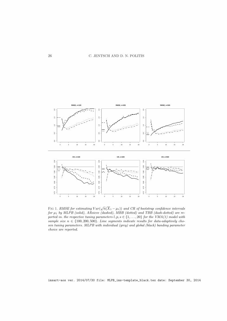
For data generated by the VMA(1) model, Figure 1 shows that the MLPBoutperforms AR sieve, MBB and TBB for adequate tuning parameter choice,that is, l ≈ 1. In this case, the MLPB behaves generally superior wrt RMSEand CR to the other bootstrap methods for all tuning parameter choices ofp and s. This was not unexpected since, by design, the MLPB can approx-imate very efficiently the covariance structure of moving average processes.Nevertheless, due to the fact that all proposed bootstrap schemes are validat least asymptotically, ARsieve gets rid of its bias with increasing order p,but at the expense of increasing variability and consequently also increasingRMSE. MLPB with data-adaptively chosen banding parameter performsquite well, where the individual choice tends to perform superior to theglobal choice in most cases. In comparison, MBB and TBB seem to performquite well for adequate block length, but they lose in terms of RMSE as wellas CR performance if the block length is chosen automatically.

The data from the VAR(1) model is highly persistent due to the coeffi-cient A11 = 0.9 near to unity. This leads to autocovariances that are ratherslowly decreasing with increasing lag and, consequently, to large variancesof

√n(X − µ). Figure 2 shows that ARsieve outperforms MLPB, MBB and

TBB wrt to CR for small AR orders p ≈ 1. This was to be expected sincethe underlying VAR(1) model is captured well by ARsieve even with fi-nite sample size. But the picture appears to be different wrt RMSE. Here,MLPB may perform superior for adequate tuning parameter choice, butthis effect can be explained by the very small variance that compensates itslarge bias in comparison to the AR sieve [not reported here] leading to a



smaller RMSE. This phenomenon is also illustrated by the poor performanceof MLPB wrt to CR for small choices of l. However, more surprising is therather good performance of the MLPB if the banding parameter is chosendata-adaptively, where the MLPB appears to be comparable to the ARsievein terms of RMSE and at least close wrt CR. Further, as observed alreadyfor the VMA(1) model in Figure 1, the individual banding parameter choicegenerally tends to outperform the global choice here again. Similarly, it canbe seen here that the performance of ARsieve worsens with increasing p atthe expense of increasing variability. The block bootstraps MBB and TBBappear to be clearly inferior to MLPB and AR sieve particularly wrt CR,but also wrt to RMSE if tuning parameters are chosen automatically.

6.2. Bootstrap performance: the effect of larger time series dimension.We consider d-dimensional realizations X1, . . . , Xn with n = 100, 200, 500from two DGPs of several dimensions. Precisely, we study first order vectormoving average processes

VMAd(1) model Xt = Aet−1 + et

and first order vector autoregressive processes

VARd(1) model Xt = AXt−1 + et

of dimension d ∈ {2, . . . , 10}, where et ∼ N (0,Σd) is a d-dimensional nor-mally distributed i.i.d. white noise process and Σ = (Σij) and A = (Aij) aresuch that

Σij =

1, i = j

0.5, |i− j| = 1

0, otherwise

and Aij =

0.9, i = j, (i+ 1)/2 ∈ N

0.5, i = j, i/2 ∈ N

−0.4, i+ 1 = j

0, otherwise

.

Observe that the VMA(1) and VAR(1) models considered in Section 6.1 areincluded in this setup for d = 2.

In Figures 3 and 4, we compare the performance of MLPB, ARsieve,MBB and TBB for the DGPs above using RMSE and CR averaged over alld time series coordinates. Precisely, we compute RMSE individually for theestimates of V ar(

√n(X i − µi)), i = 1, . . . , d and plot the averages in the

upper half of Figures 3 and 4. Similarly, we plot averages of individuallycalculated CR of bootstrap confidence intervals for µi, i = 1, . . . , d in thelower halfs. All tuning parameters are chosen data-based and optimal as



described in Section 6.1 and to reduce computation time, the less demandingalgorithm as described in Section 5.4 with S = dn/500 is used.

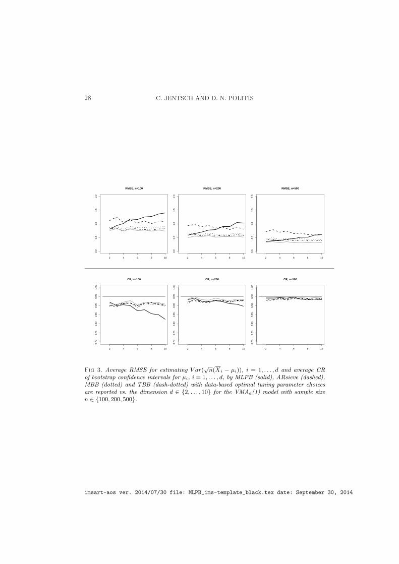
For the VMA(1) DGPs in Figure 3, the MLPB with individual bandingparameter choice outperforms the other approaches essentially for all timeseries dimension under consideration wrt to averaged RMSE and CR. Inparticular, larger time series dimensions do not seem to have a large effecton the performance of all bootstraps for the VMA(1) DGPs with the onlyexception of the MLPB with global banding parameter choice. In particular,the latter is clearly inferior in comparison to the MLPB with individuallychosen banding parameter, which might be explained by sparsity of thecovariance matrix Γdn.

In Figure 4, for the VAR(1) DGPs, the picture is different to the VMA(1)case above. The influence of larger time series dimension on RMSE (andless pronounced for CR) performance is much more pronounced and clearlyvisible. In particular, the RMSE blows up with increasing dimension d forall four bootstrap methods, which is due to the also increasing variance ofthe process. Note that the zig-zag shape of the RMSE curves is due to theback and forth switching from 0.9 to 0.5 on the diagonal of A. As already ob-served for the VMA(1) DGPs, the MLPB with individual banding parameterchoice again performs best over essentially all time series dimensions wrt toaverage RMSE and average CR. In particular, MLPB with individual choiceis superior to the global choice. Here, the good performance of the MLPBis somewhat surprising as the VAR(1) DGPs have rather slowly decreas-ing autocovariance structure, where we expected an ARsieve to be moresuitable.

ACKNOWLEDGEMENTS

The research of the first author was supported by a fellowship within thePhD-Program of the German Academic Exchange Service (DAAD) whenCarsten Jentsch was visiting the University of California, San Diego, USA.The research of Dimitris Politis was partially supported by NSF grants DMS13-08319 and DMS 12-23137. The authors thank Timothy McMurry for hishelpful advice on the univariate case and three anonymous referees and theeditor who helped to significantly improve the presentation of the paper.

SUPPLEMENTARY MATERIAL

Additional proofs, simulations and a real data example

(doi: 10.1214/00-AOASXXXXSUPP; .pdf). In the supplementary materialwe provide proofs, additional supporting simulations and an application ofthe MLPB to German stock index data.


http://dx.doi.org/10.1214/00-AOASXXXXSUPP


The supplementary material to this paper is also abvailable online athttp://www.math.ucsd.edu/~politis/PAPER/MLPBsupplement.pdf

REFERENCES

[1] Brillinger, D. (1981). Time Series: Data Analysis and Theory. Holden-Day, SanFrancisco.

[2] Brockwell, P.J. and Davis, R.A. (1988). Simple consistent estimation of the coef-ficients of a linear filter. Stochastic Processes and Their Applications 22, 47–59.

[3] Brockwell, P.J. and Davis, R.A. (1991). Time series: theory and methods. 2nd ed.Springer-Verlag, Berlin.

[4] Brockwell, P.J. and Mitchell, H. (1997). Estimation of the coefficients of a mul-tivariate linear filter using the innovations algorithm. J. Time Ser. Anal. 18 157–179.

[5] Buhlmann, P. (1997). Sieve bootstrap for time series. Bernoulli 3 123–148.[6] Buhlmann, P. (2002). Bootstraps for Time Series. Statist. Sci. 17 52–72.[7] Cai, T., Ren, Z., and Zhou, H. (2013). Optimal Rates of Convergence for Estimating

Toeplitz Covariance Matrices. Probab. Theory Relat. Fields 156 101–143.[8] Davidson, J. (1994). Stochastic Limit Theory. Oxford University Press, New York.[9] Dedecker, J., Doukhan, P., Lang, G., Leon, J.R.R., Louhichi, S., and Prieur,

C. (2007). Weak dependence. With examples and applications. Lecture Notes in Statis-tics 190. Springer, New York.

[10] Doukhan, P. (1994). Mixing: Properties and examples. Lecture Notes in Statistics85. Springer, New York.

[11] Goncalves, S. and Kilian, L. (2007). Asymptotic and bootstrap inference forAR(∞) processes with conditional heteroskedasticity. Econometric Reviews 26 609–641.

[12] Hannan, E.J. (1970). Multiple Time Series.Wiley, New York.[13] Hardle, W., Horowitz, J., and Kreiss, J.-P. (2003). Bootstrap Methods for Time

Series. Int. Statist. Rev. 71 435–459.[14] Horn, R.A. and Johnson, C.R. (1990). Matrix analysis. Cambridge University

Press, New York.[15] Jentsch, C. and Politis, D.N. (2013). Valid resampling of higher order statistics

using linear process bootstrap and autoregressive sieve bootstrap. Commun. Stat.,Theory Methods 42 1277–1293.

[16] Jentsch, C. and Politis, D.N. (2014). Supplement to ‘Covariance matrix estima-tion and linear process bootstrap for multivariate time series of possibly increasingdimension”.

[17] Kreiss, J.-P. (1992). Bootstrap Procedures for AR(∞) Processes. In: Bootstrappingand Related Techniques. Jockel, K. H., Rothe, G., Sender, W., eds. Lecture Notes inEconomics and Mathematical Systems 376, Heidelberg: Springer-Verlag, pp. 107–113.

[18] Kreiss, J.-P. (1999). Residual and Wild Bootstrap for Infinite Order Autoregression.Unpublished manuscript.

[19] Kreiss, J.-P. and Paparoditis, E. (2011). Bootstrap for dependent data: a review.J. Korean Statist. Soc. 40 357–378.

[20] Kreiss, J.-P., Paparoditis, E., and Politis, D. N. (2011). On the range of validityof the autoregressive sieve bootstrap. Ann. Statist. 39 2103-2130.

[21] Kunsch, H.R. (1989). The Jackknife and the Bootstrap for General Stationary Ob-servations. Ann. Statist. 17 1217–1241.

[22] Lahiri, S.N. (2003). Resampling methods for dependent data. Springer, New York.



[23] Lewis, R. and Reinsel, G. (1985). Prediction of multivariate time series of autore-gressive model fitting. Journal of Multivariate Analysis. 16 393–411

[24] Liu, R.Y. and Singh, K. (1992). Moving blocks jackknife and bootstrap capture weakdependence. In: Exploring the Limits of Bootstrap (Eds.: LePage, R. and Billard, L.),pp. 225–248. Wiley, New York.

[25] McMurry, T.L. and Politis, D.N. (2010). Banded and tapered estimates for auto-covariance matrices and the linear process bootstrap. J. Time Ser. Anal. 31 471–482.CORRIGENDUM: J. Time Ser. Anal. 33, 2012.

[26] Paparoditis, E. (2002). Frequency Domain Bootstrap for Time Series. In EmpiricalProcess Techniques for Dependent Data (H. Dehling, T. Mikosch and M. Sorensen,eds.) 365-381. Birkhauser, Boston.

[27] Politis, D.N. (2001). On nonparametric function estimation with infinite-order flat-top kernels, in Probability and Statistical Models with applications, Ch. Charalambideset al. (Eds.), pp. 469–483. Chapman and Hall/CRC, Boca Raton.

[28] Politis, D.N. (2003a). The impact of bootstrap methods on time series analysis.Statistical Science 18 219–230.

[29] Politis, D.N. (2003b). Adaptive bandwidth choice. J. Nonparametric Statist. 15

517–533.[30] Politis, D.N. (2011). Higher-order accurate, positive semi-definite estimation of

large-sample covariance and spectral density matrices. Econometric Theory 27 703–744.

[31] Politis, D.N. and Romano, J.P. (1992). A General Resampling Scheme for Trian-gular Arrays of alpha-mixing Random Variables with Application to the Problem ofSpectral Density Estimation. Ann. Statist. 20 1985–2007.

[32] Politis, D.N. and Romano, J.P. (1994). Limit Theorems for Weakly DependentHilbert Space Valued Random Variables with Applications to the Stationary Boot-strap. Statistica Sinica 4 461–476.

[33] Politis, D.N. and Romano, J.P. (1995). Bias-Corrected Nonparametric SpectralEstimation. J. Time Ser. Anal. 16 67–104.

[34] Rissanen, J. and Barbosa, L. (1969). Properties of infinite covariance matrices andstability of optimum predictors. Information Sci. 1 221–236.

[35] Shao, X. (2010). The dependent wild bootstrap. J. Am. Stat. Assoc. 105 218–235.[36] Wu, W.B. and Pourahmadi, M. (2009). Banding sample autocovariance matrices

of stationary processes. Statistica Sinica 19 1755–1768.

C. Jentsch

Department of Economics

University of Mannheim

L7, 3-5

68131 Mannheim

Germany

E-mail: [email protected]

D. N. Politis

Department of Mathematics

University of California, San Diego

La Jolla, CA 92093-0112

USA

E-mail: [email protected]


mailto:[email protected]

mailto:[email protected]


0 5 10 15 20

0.0

0.5

1.0

1.5

2.0

RMSE, n=100

0 5 10 15 20

0.0

0.5

1.0

1.5

2.0

RMSE, n=200

0 5 10 15 200.

00.

51.

01.

52.

0

RMSE, n=500

0 5 10 15 20

0.70

0.75

0.80

0.85

0.90

0.95

1.00

CR, n=100

0 5 10 15 20

0.70

0.75

0.80

0.85

0.90

0.95

1.00

CR, n=200

0 5 10 15 20

0.70

0.75

0.80

0.85

0.90

0.95

1.00

CR, n=500

Fig 1. RMSE for estimating V ar(√n(X1 −µ1)) and CR of bootstrap confidence intervals

for µ1 by MLPB (solid), ARsieve (dashed), MBB (dotted) and TBB (dash-dotted) are re-ported vs. the respective tuning parameters l, p, s ∈ {1, . . . , 20} for the VMA(1) model withsample size n ∈ {100, 200, 500}. Line segments indicate results for data-adaptively cho-sen tuning parameters. MLPB with individual (grey) and global (black) banding parameterchoice are reported.



0 5 10 15 20

020

4060

80

RMSE, n=100

0 5 10 15 20

020

4060

80

RMSE, n=200

0 5 10 15 20

020

4060

80

RMSE, n=500

0 5 10 15 20

0.5

0.6

0.7

0.8

0.9

1.0

CR, n=100

0 5 10 15 20

0.5

0.6

0.7

0.8

0.9

1.0

CR, n=200

0 5 10 15 20

0.5

0.6

0.7

0.8

0.9

1.0

CR, n=500

Fig 2. As in Figure 1, but with VAR(1) model.



2 4 6 8 10

0.0

0.5

1.0

1.5

2.0

RMSE, n=100

2 4 6 8 10

0.0

0.5

1.0

1.5

2.0

RMSE, n=200

2 4 6 8 10

0.0

0.5

1.0

1.5

2.0

RMSE, n=500

2 4 6 8 10

0.70

0.75

0.80

0.85

0.90

0.95

1.00

CR, n=100

2 4 6 8 10

0.70

0.75

0.80

0.85

0.90

0.95

1.00

CR, n=200

2 4 6 8 10

0.70

0.75

0.80

0.85

0.90

0.95

1.00

CR, n=500

Fig 3. Average RMSE for estimating V ar(√n(Xi − µi)), i = 1, . . . , d and average CR

of bootstrap confidence intervals for µi, i = 1, . . . , d, by MLPB (solid), ARsieve (dashed),MBB (dotted) and TBB (dash-dotted) with data-based optimal tuning parameter choicesare reported vs. the dimension d ∈ {2, . . . , 10} for the VMAd(1) model with sample sizen ∈ {100, 200, 500}.



2 4 6 8 10

050

010

0015

00

RMSE, n=100

2 4 6 8 10

050

010

0015

00

RMSE, n=200

2 4 6 8 10

050

010

0015

00

RMSE, n=500

2 4 6 8 10

0.5

0.6

0.7

0.8

0.9

1.0

CR, n=100

2 4 6 8 10

0.5

0.6

0.7

0.8

0.9

1.0

CR, n=200

2 4 6 8 10

0.5

0.6

0.7

0.8

0.9

1.0

CR, n=500

Fig 4. As in Figure 3, but with VARd(1) model.


covariance matrix estimation and linear process bootstrap

Documents