3

SAND96-1169Unlimited Release

Printed May 17, 1996

Discrete Optimization of Isolator Locations

for Vibration Isolation Systems:

an Analytical and Experimental Investigation

E. R. Ponslet and M. S. EldredStructural Dynamics Department

Sandia National LaboratoriesAlbuquerque, New Mexico 87185-0439

Abstract

An analytical and experimental study is conducted to investigate the effect ofisolator locations on the effectiveness of vibration isolation systems. The study usesisolators with fixed properties and evaluates potential improvements to the isolationsystem that can be achieved by optimizing isolator locations.

Because the available locations for the isolators are discrete in this application, aGenetic Algorithm (GA) is used as the optimization method. The system is modeled inMATLAB and coupled with the GA available in the DAKOTA optimization toolkitunder development at Sandia National Laboratories. Design constraints dictated byhardware and experimental limitations are implemented through penalty functiontechniques. A series of GA runs reveal difficulties in the search on this heavilyconstrained, multimodal, discrete problem. However, the GA runs provide a variety ofoptimized designs with predicted performance from 30 to 70 times better than a baselineconfiguration. An alternate approach is also tested on this problem: it uses continuousoptimization, followed by "rounding" of the solution to neighboring discreteconfigurations. Results show that this approach leads to either infeasible or poor designs.

Finally, a number of "optimized" designs obtained from the GA searches aretested in the laboratory and compared to the baseline design. These experimental resultsshow a 7 to 46 times improvement in vibration isolation from the baseline configuration.

SAND96-116905/17/96

4

Acknowledgments

This work was funded by DOE through Sandia National Laboratories undercontract number AP-5115 with AMPARO Corporation, Santa Fe, NM.

The authors wish to thank David Martinez for initiating support for this research,Clay Fulcher for his advice and assistance with many practical problems, Bill Hart for hisassistance with the genetic algorithm in DAKOTA, and Tom Rice for his invaluable helpin preparing the experimental setup.

SAND96-116905/17/96

5

Content

1. Introduction ..................................................................................................................... 82. System Description........................................................................................................ 103. Optimization Problem ................................................................................................... 124. Modeling ....................................................................................................................... 13

4.1 Suspended Rigid Body Modeling ............................................................................ 134.2 Mass Properties ........................................................................................................ 144.3 Stiffness and Damping ............................................................................................. 14

4.3.1 Airbags............................................................................................................... 144.3.2 Steel Springs ...................................................................................................... 15

4.4 Analysis Code .......................................................................................................... 164.4.1 Objective Function Calculation ......................................................................... 164.4.2 Constraint Evaluation ........................................................................................ 16

5. Baseline Design............................................................................................................. 176. Optimization Techniques .............................................................................................. 18

6.1 Random Search ........................................................................................................ 186.2 Genetic Algorithm.................................................................................................... 18

6.2.1 Description......................................................................................................... 186.2.2 Defining the Chromosome (Coding) ................................................................. 196.2.3 Selection Operator ............................................................................................. 216.2.4 Crossover Operator............................................................................................ 216.2.5 Mutation Operator ............................................................................................. 226.2.6 Constraint Enforcement ..................................................................................... 23

6.3 Rounding of Continuous Optimum.......................................................................... 257. Optimization Results ..................................................................................................... 26

7.1 Genetic Algorithm and Random Search .................................................................. 267.2 Rounding of Continuous Optimum.......................................................................... 297.3 A Look at the Design Space..................................................................................... 30

8. Experimental Results..................................................................................................... 329. Conclusions ................................................................................................................... 33

9.1 Optimum Isolation System Design .......................................................................... 339.2 Discrete Optimization .............................................................................................. 34

10. References ................................................................................................................... 34

SAND96-116905/17/96

6

List of Figures

Figure 1 Vibration isolation systems.................................................................................. 8Figure 2 Typical transmission characteristics of isolation system. .................................... 8Figure 3 Improving isolation by softening the isolators..................................................... 9Figure 4 Non-generic isolation problem........................................................................... 10Figure 5 Experimental vibration isolation setup. ............................................................. 11Figure 6 Steel spring isolator............................................................................................ 11Figure 7 Vibration isolation design problem.................................................................... 12Figure 8 Locations of isolators in baseline design. .......................................................... 17Figure 9 Transmissibility of baseline design.................................................................... 17Figure 10 Random search technique. ............................................................................... 18Figure 11 Classical genetic algorithm. ............................................................................. 19Figure 12 Various ways of coding isolator locations into a "chromosome" for a genetic

algorithm..................................................................................................................... 20Figure 13 Ranking selection operator............................................................................... 21Figure 14 Non-averaging 2-point crossover operator....................................................... 22Figure 15 Mutation operator............................................................................................. 23Figure 16 Design problem with disjoint feasible space.................................................... 23Figure 17 A simple repair operator for the corner constraint. .......................................... 24Figure 18 Penalty function approach used in this application; the shaded area is

infeasible..................................................................................................................... 25Figure 19 Using continuous approximation followed by rounding to nearby discrete

solution. ...................................................................................................................... 26Figure 20 Comparison of genetic algorithm and random search results using the same

number of function evaluations (105). Designs shown are the best found for each run.27Figure 21 GA optimized designs and their transmissibilities at 50 Hz (in µin/sec/lb),

compared to baseline configuration............................................................................ 28Figure 22 Transmissibility curves of optimized designs compared to baseline

configuration (model predictions). ............................................................................. 29Figure 23 Results from continuous optimization and rounding. ...................................... 29Figure 24 Rounding a continuous optimum to neighboring discrete solutions................ 30Figure 25 Two-dimensional cut through the design space obtained by moving one

isolator in both directions; for clarity, the constrained objective plot only shows steppenalties. ..................................................................................................................... 31

Figure 26 Design space cross section showing unconstrained objective, discrete grid,contour lines, constraint boundaries, feasible domain (shaded), and feasible discretedesigns with their transmissibilities; the + shows the discrete optimum................... 32

Figure 27 Experimental transmissibilities at 50 Hz of baseline and optimized designs,compared to analytical predictions. ............................................................................ 33

SAND96-116905/17/96

7

List of Tables

Table 1 Experimental modes of seismic base on airbags ................................................. 14Table 2 Seismic base on air springs; analytical and experimental modes........................ 15Table 3 Experimental modes of optical table on 4 spring isolators. ................................ 15Table 4 Optical table on 4 spring isolators; analytical and experimental modes. ............ 15

SAND96-116905/17/96

8

1. Introduction

Vibration isolation systems are used in a wide variety of applications to reducetransmission of mechanical vibrations generated by noisy components or carried by theenvironment to a sensitive device. Examples include isolation of a laser table from floor-borne seismic disturbances, isolation of a car or airplane body from engine vibrations, andsuspension systems of vehicles.

Isolation is achieved by inserting soft mechanical links (“isolators”) between thesubsystem containing the source of the disturbances and the subsystem to be isolated.Based on the relative sizes of these subsystems, two classes of isolation systems can bedistinguished (Fig. 1).

T

Floor Vibrations

Quiet Device

T

Quiet Floor

VibratingDevice

Figure 1 Vibration isolation systems.

In the first situation (left side of Fig. 1), the environment is isolated fromvibrations created by a piece of machinery. A typical example is the isolation of a carbody from vibrations caused by the engine. In the other, a sensitive device is protectedfrom disturbances carried by its supporting structure. Isolation of a laser table from floorborne vibrations is a common example. In both cases, the effectiveness of the isolationsystem can be examined in terms of transmissibility functions, T, in the frequencydomain. In the first class of systems, these transmissibilities can be expressed as ratios ofexcitation forces to forces transmitted to the floor. In the second class, they are expressedas ratios of component of floor motion to component of device motion. Note that mixedformulations are also possible. Whatever exact definition is used for T, its magnitudetypically resembles the curve shown in Fig. 2.

dB(T)

log(Frequency)

isolation range

suspensionmodes

flexiblemodes

Figure 2 Typical transmission characteristics of isolation system.

SAND96-116905/17/96

9

Three regions can be distinguished in the figure. At “low” frequencies, resonantpeaks corresponding to the suspension modes are observed. There is no isolation in thisband (in fact there is amplification). Damping is usually designed into the isolators tolimit the amplitudes of these peaks and avoid large responses to transients. At the “high”end of the spectrum, flexible modes of the device and/or supporting structure themselvesproduce other resonant peaks. In a properly designed isolation system, those twofrequency ranges are separated by a wide “isolation band” where transmission decaysrapidly with frequency (about -40dB/decade for a lightly damped, single stage system). Aproperly designed system will “see” most of the disturbance energy occur in this band.

Because of the sharp decay in the isolation band, the traditional designmethodology focuses primarily on minimizing the stiffnesses of the individual isolators.This lowers the frequencies of the suspension modes and results in a corresponding dropin transmission in the isolation band (Fig. 3). The configuration of the complete system,in particular the number, locations, and orientations of the isolators, receives littleattention in this approach. Actually, the system configuration is often designed to ensuredecoupling between translations and rotations in the suspension modes and simplify theanalysis[1].

Figure 3 Improving isolation by softening the isolators.

This approach is justified for “generic” isolation problems. Namely, when thelocation, direction, amplitude, or frequency content of the disturbances are not wellknown and/or when no particular point on the isolated device more critically requiresisolation than others. An example of a generic problem is that of isolating a laser tablefrom floor vibrations: data will often not be available to accurately characterize thedisturbance and the designer of the isolation system has no knowledge of whatexperiment will be performed on the table. In such cases, a generic isolation system (with4 isolators, one in each corner for example) is appropriate.

However, in some applications, the disturbance(s) are very well known (rotatingmachinery, for example) and residual motion is critical at one or a few specificpoints/directions on the isolated device. As an example, consider an isolation systemdesigned to prevent excessive transmission of vibrations from a cryocooler to a telescopemounted on a satellite structure (Fig. 4). Clearly, the source of the disturbance is wellknown in direction, amplitude, and frequency content. Also, to minimize jitter, residualtilting vibrations of the telescope must be minimized. Vibrations at other points/directionsin the system are less critical. In other applications, the critical point/direction might bethe location of a vibration-sensitive component or points/directions of strong dynamic

SAND96-116905/17/96

10

coupling with an elastic sub-system. In all such cases, it is expected that locations andorientations of the isolators will have a substantial effect on the isolation effectiveness[2].

T

Figure 4 Non-generic isolation problem.

The present study examines this question in more detail. The authors consider thedesign of a 3-isolator system to minimize transmission of well characterized floor-borneperturbations to a specific point and direction on an optical table. The number and type ofisolators used is fixed and their locations under the table are optimized. The optimizeddesigns are compared to a baseline, generic configuration. These designs are then testedin the lab to validate the approach.

Because our optical table provides only a discrete grid of mounting holes for theisolators, the design variables of the optimization problem are discrete and theoptimization is performed with SGOPT’s[3] Genetic Algorithm (GA) available in theDAKOTA [4] optimization toolkit under development at Sandia National Laboratories.

The goal of the study is twofold: first, investigate the potential of optimization inimproving the performance of vibration isolation systems and second, by exercising theGA with a real-life problem, hopefully identify critical directions for future GA researchand development efforts.

2. System Description

The experimental vibration isolation setup (Fig. 5) consists of a stainless steelhoneycomb sandwich optical table (Newport[5], model RS4000-36-8) measuringapproximately 48 by 36 by 8.5 inches and weighing approximately 815 lbs. The table isresting on 3 steel coil spring isolators (custom designed, using springs from AssociatedSpring-Raymond[6], model CV2000-2500-365) whose locations under the table are thefocus of the optimization. This system is in turn resting on a large, solid aluminumseismic mass (custom-made, approximately 70 by 48 by 12 inches, 4085 lb.), itselfisolated from the lab floor by four air bags (Firestone Airmount isolators[7], model224C). Note that the seismic mass will actually be considered the “floor” in this problem.The air bag suspension is there to eliminate any unknown disturbances from theexperiment but will not be part of the optimization problem. The suspension frequenciesof the system on these airbags range from about 1.0 to 2.5 Hz.

SAND96-116905/17/96

11

Z

Y

X

Optical Table

Shaker

Accelerometer

Adapter Plates

Seismic Base

Load CellLifter

Airbag

Accelerometers

Mounting Hole

Z

Y

X

Figure 5 Experimental vibration isolation setup.

The bottom of the optical table and the top of the seismic base are fitted withidentical aluminum adapter plates featuring matching arrays of 6 by 8 threaded holes (ona 6 in. grid). The spring isolators are attached to those holes with threaded rods andaluminum end-plates as shown in Fig. 6. Note that because the springs are simply restingin the end-plates, the isolators can only take compressive forces.

coil spring

end plate

Figure 6 Steel spring isolator.

Four hydro-pneumatic lifters are attached to the seismic block, allowingconvenient access to the isolators. The four corners of the aluminum adapter plateattached to the seismic block are machined to provide clearance for the lifters. Thiseliminates 4 of the 48 possible isolator mounting locations.

SAND96-116905/17/96

12

Both the seismic base and the optical table are fully instrumented for 6 d.o.f.motion pickup for system identification and model validation purposes (see Section 4.3).Four sets of 3 accelerometers (Endevco[8], model 7751-500mV/g) are mounted near thefour corners of the seismic base as seen in Fig. 5. The optical table is equipped with 5triaxial accelerometers (Endevco[8], model 63-500mV/g), embedded in the aluminumadapter plate near the four corners and the center. All accelerometers are powered by 12-channel signal conditioners (PCB[9], model 483A10). In addition, a high sensitivityseismic accelerometer (Wilcoxon Research[10], model 731, 10,000 mV/in/sec. in velocitymode) measures residual vibration at the critical point, near the front left corner of theoptical table.

The “floor” (seismic base) is excited near its front right corner (Figure 4) by anelectromagnetic shaker (MB Dynamics[11], model Modal 50A). The excitation force ismeasured by a piezoelectric load cell (PCB[9], model 208A03, 10mV/lb.).

3. Optimization Problem

The vibration isolation problem is shown schematically in Fig. 7. As mentionedpreviously, the goal is to find optimal locations for 3 steel spring isolators between theoptical table and the seismic base. The number of isolators was set to 3 to minimizeuncertainties in the experimental setup that would occur due to static indeterminacy with4 or more isolators. By design, only 6x8=48 discrete locations are available for theseisolators. Four of those locations (at the corners) are not available (see Section 2).

Quiet Location & Direction( V, vertical velocity)

Perturbation(F, 50 Hz sine)

Seismic Base (“floor”)

6 x 8 DiscreteLocations

Optical Table

3 Isolators

Lab Floor

T = V / F

Figure 7 Vibration isolation design problem.

For simplicity, and to reduce computational expenses in the simulations, thedisturbance is a pure sinusoidal vertical force F at a frequency of 50 Hz. This frequencywas chosen to be within the isolation band, i.e. much higher than that of the suspensionmodes of the optical table but well below the frequency of the lowest elastic modes (150to 200 Hz). It will be shown that the use of a single target frequency instead of a wideband does not limit the improvements to that single frequency. Instead, the optimizeddesigns actually have improved performance across the isolation range.

SAND96-116905/17/96

13

The objective is to minimize the residual vertical velocity V at a target location onthe table (Figure 7), in response to a given amplitude of perturbation force F. Thisamounts to minimizing the transfer function T = V/F (µin/sec/lb) from the excitationforce to the residual velocity. This function T will be referred to as transmissibility in theremainder of this report. The locations of the excitation and the critical point were chosento create asymmetry in the problem. This is expected to lead to non-intuitive, asymmetricoptimal locations for the isolators, in sharp contrast to a baseline configuration.

Practical limitations dictate a number of design constraints on this problem (theimplementation of those constraints is explained in more detail in the next section):• Depending on how the isolator locations are coded into design variables, it may be

necessary to enforce the condition that the 4 locations at the corners of the 6x8 gridare not used.

• There cannot be more than one isolator at any given grid location.• The isolators cannot be aligned on a straight line because the table would then be

unstable. Note that, with 3 isolators, this condition also takes care of the previous one:if any two isolators are at the same location they are also on a straight line with thethird one.

• Also, since softer isolation generally implies better performance (see Section 1) theremay be a tendency for the optimizer to generate designs with very low naturalfrequencies (by placing the isolators very close to each other for example). This isundesirable in practice because such designs would have very large transientresponses to impact and handling loads. To prevent this, a lower limit of 4.0 Hz isenforced on the first natural frequency of the optical table on its isolators. Note thatthis value also ensures decoupling with the suspension modes of the seismic base onits airbags (1 to 2.5 Hz).

• Because the springs are not attached to their end-plates, the static gravitational loadon each isolator must be compressive.

• The static deflections of the springs cannot exceed an upper limit beyond which thesprings might not be linear or might be compressed to their solid length. This limitwas set to 0.5 in.

The discrete nature of the design variables (isolator locations) calls for the use ofspecialized optimization techniques. An approach based on a genetic algorithm will beexamined in this study and compared to other techniques. It will be shown that the use ofclassical continuous optimization techniques followed by rounding of the solution is notappropriate.

4. Modeling

4.1 Suspended Rigid Body Modeling

The lowest “flexible” modes in the system occur at frequencies of about 150 to200 Hz. They correspond to resonances of tuned vibration absorbers which are embeddedin the optical table. At frequencies well below these flexible modes (say from 0 to100Hz), the system can be approximated as a set of 2 rigid bodies (seismic base andoptical table) connected by 3-dimensional, linear springs with viscous damping (airbags

SAND96-116905/17/96

14

and spring isolators). Each rigid body is given 6 degrees of freedom and defined by itsmass and inertia tensor. The springs are defined by stiffnesses (kx, ky, kz) and dampingcoefficients (cx, cy, cz) in 3 mutually orthogonal directions, parallel to the global referencedirections X, Y, and Z of Fig. 5. For the system at hand, we have kx=ky=kshear, kz=kaxial,cx=cy=cshear, and cz=caxial because of axisymmetry of both the airbags and the steelsprings. Bending and torsional stiffnesses of the springs were neglected.

4.2 Mass Properties

Mass properties for most components (seismic base, adapter plates, airbag adapterblocks, etc.) were obtained from Pro-Engineer[12] models. The lifters were weighed andtheir inertia tensors were approximated based on uniform density assumptions in a Pro-Engineer geometric model. The optical table posed special problems: because of thepresence of embedded tuned vibration absorbers of unknown properties (accurate datacould not be obtained from the manufacturer), the mass properties could not bedetermined analytically and were instead measured by the Mass Property Laboratory atSandia National Laboratories. The center of mass of the table was found to be offset by1.72 in. in the negative Y direction from its geometric center (due to uneven distributionof tuned dampers).

4.3 Stiffness and Damping

4.3.1 Airbags

The stiffness of an airbag is almost exactly proportional to the static axial load(the natural frequency of a 1 d.o.f. system made of an airbag and a mass is approximatelyindependent of the magnitude of the mass). Initial data for axial stiffness versus axialload was obtained from the manufacturer’s catalog[7] and can be approximated as

kaxial = 66.51 + 0.4047 P,

where P is the axial static load in lb and kaxial is in lb/in. Shear stiffnesses were notavailable. Modal tests were then performed on the seismic mass alone, supported by theairbags (the optical table and springs were removed for this test). Natural frequencies andmodal damping ratios were extracted form those measurements and are listed in Table 1.

Mode # Frequency [Hz] Damping [%]1 0.961 2.95 shear along X (+ rocking around Y)2 1.145 3.23 shear along Y (+ rocking around X)3 1.519 3.36 twist around Z4 2.161 0.82 symmetric up/down along Z5 2.464 1.61 rocking around Y6 2.467 1.28 rocking around X

Table 1 Experimental modes of seismic base on airbags

Mode 4 (pure up and down motion) was used to adjust the axial stiffness anddamping (catalog values for stiffness was scaled by 1.0154) and mode 3 (pure twistingmotion around Z, straining the airbags in pure shear) provided the ratio of shear to axialstiffness (kshear/kaxial = 0.4611) and the shear damping. With those values, the modelpredictions compare reasonably well with the experiment (Table 2).

SAND96-116905/17/96

15

Frequency [Hz] Damping ratio [%]exp. anal. exp. anal.

shear along X (+ rocking around Y) 0.961 1.192 2.95 1.70shear along Y (+ rocking around X) 1.145 1.333 3.23 2.39twist around Z 1.519 1.519 3.36 3.36symmetric up/down along Z 2.161 2.161 0.82 0.82rocking around Y 2.464 2.489 1.61 2.90rocking around X 2.467 2.479 1.28 1.97

Table 2 Seismic base on air springs; analytical and experimental modes.

4.3.2 Steel Springs

With the assumption of linearity, the dynamic axial and shear stiffnesses of a coilspring are independent of static loads. An initial value kaxial = 3816 lb/in was obtainedfrom the manufacturer[6]. The shear stiffness was not available. Modal tests wereperformed on the optical table resting on 4 spring isolators, symmetrically arrangedaround its geometric center. The airbags supporting the seismic base were replaced withstiff support blocks for those tests. Measured natural frequencies and modal dampingratios are listed in Table 3.

Mode # Frequency [Hz] Damping [%]1 7.199 0.16 shear along X left side2 8.007 0.41 shear along X right side3 8.456 0.22 shear along Y (+ rocking X)4 12.121 0.15 rocking around Y5 12.885 0.16 up/down left side6 14.551 0.21 up/down right side

Table 3 Experimental modes of optical table on 4 spring isolators.

Frequency [Hz] Damping ratio [%]exp. anal. exp. anal.

shear along X left side 7.199 7.375 0.16 0.22shear along X right side 8.007 8.020 0.41 0.26shear along Y (+ rocking X) 8.456 8.279 0.22 0.27rocking around Y 12.121 12.203 0.15 0.25up/down left side 12.885 12.897 0.16 0.17up/down right side 14.551 14.370 0.21 0.16

Table 4 Optical table on 4 spring isolators; analytical and experimentalmodes.

The simple analytical technique used to identify airbag stiffnesses and dampingscannot be used here because of the absence of pure up/down or shear modes. Instead, aparameter identification optimization problem was formulated that minimizes a weightedsum of squares of errors on natural frequencies and damping ratios. Four parameters wereadjusted to minimize this error: axial stiffness kaxial and damping caxial, and shear stiffnesskshear and damping cshear. The minimization was performed using OPT++[13] conjugate

SAND96-116905/17/96

16

gradient optimizer in DAKOTA. The results lead to a correction factor of 1.04 on thecatalog value for kaxial, a ratio kshear/ kaxial = 0.41, and damping coefficients caxial = 0.13and cshear = 0.18. These values achieve good analytical-experimental match (Table 4).

4.4 Analysis Code

The rigid body equations of motion were coded into a set of M-files inMATLAB[14]. For the optimization, interfacing with DAKOTA† was done directly(without the use of input and output filters[4]) since the MATLAB code could be designedto exchange information (design variables and objective function) in the DAKOTAcompatible format.

4.4.1 Objective Function Calculation

The transmissibility T at a single frequency of 50 Hz (see Section 2) is calculatedby solving the (12x12) set of linear dynamic equations for that frequency.

4.4.2 Constraint Evaluation

• corner constraints: simple checks are performed for each isolator location. ThreeBoolean constraints g1, g2, g3 are defined as

gi = < is isolator # i at corner? >, i=1,…,3, boolean constraints.• alignment constraint: since natural frequencies are needed for the 4Hz limit in thestability constraint, alignment was checked by monitoring the value of the first naturalfrequency f1 (out of 12) of the system. A value of zero indicates alignment (or more than 1spring at any location). To account for numerical roundoffs, a threshold value of 0.01 Hzwas used. This defines the 4th Boolean constraint:

g4 = < f1 < 0.01 Hz ? > , boolean constraint.Note that if this constraint is violated, the system’s stiffness matrix is nearly singular andstatic equilibrium cannot be computed. Also, there is a switch in the order of the naturalfrequencies because the first natural frequency is now associated with the upper systeminstead of being a seismic base suspension mode (which is also why the alignmentconstraint is treated separately from the stability constraint). For these reasons, allfollowing constraints g5…g11 are evaluated only if g4 is false.• stability constraint: As mentioned earlier, the upper system natural frequencies arerequired to be above 4 Hz, i.e.

g5 = 1 - f7 /4.0 Hz < 0, real constraint,where f7 is the first natural frequency of the upper half of the system (because the first 6frequencies correspond to the lower half, i.e. the seismic mass on its airbags).• compression constraint: with 3 isolators, the upper table is statically determinate sothat reaction loads can be readily computed by solving 3 equilibrium equations. Threeconstraints are formulated to guarantee that the loads are compressive:

g5+i = Pi < 0, i=1,…,3, real constraints,where Pi is the static load on spring #i (positive in traction).

† DAKOTA is an object-oriented C++ toolkit for interfacing broad libraries of optimization methods (e.g.NLP, GA’s, coordinate pattern search) with engineering applications in a variety of disciplines.

SAND96-116905/17/96

17

• static deflection constraint: three constraints enforce that the static deflections δi ofthe springs remain below a limit δmax = 0.5 in.:

g8+i = δi / δmax - 1 < 0, i=1,…,3 , real constraints.

5. Baseline Design

Before optimizing the isolation system, we first define a generic, baselineconfiguration. It will be used as a point of comparison to evaluate improvements achievedby optimization. This baseline configuration is generated following the generic designapproach described in Section 1: the three isolators are placed symmetrically around thecenter of mass of the isolated body (the optical table). Because of the coarse discrete gridof mounting holes for the isolators, perfect symmetry cannot be achieved. The selectedlocations are shown in Fig. 8.

V

F

Top View

Figure 8 Locations of isolators in baseline design.

Note that, without prior analysis, a configuration similar to that of Fig. 8 wouldprobably be used in practice. This study will show that other configurations can be foundthat lead to much superior performance.

The transmissibility predicted by the MATLAB model for this design is plotted inFigure 9. A number of resonant peaks corresponding to suspension modes can be seen atfrequencies up to about 15 Hz. At higher frequencies, the transmissibility decays rapidlyand reaches T = 21.22 µin/sec/lb at the 50 Hz target frequency.

frequency (Hz)

1

100

10000

1000000

0 20 40 60 80 100

f = 50 Hz

T = 21.22

T = V/F (µin/sec/lb.)

Figure 9 Transmissibility of baseline design.

SAND96-116905/17/96

18

Flexible modes are absent from the figure because first, they are not represented in therigid body/spring model and second, they start at frequencies of about 150 Hz.

It should be noted that the performance of this design is very representative of thisparticular isolation system: Monte Carlo simulations with 1000 random configurationsshow that the average transmissibility of feasible designs is 21.1 µin/sec/lb, almostexactly equal to that of the baseline design.

6. Optimization Techniques

Three optimization techniques are applied to this discrete problem: randomsearch, genetic algorithm (GA), and continuous optimization followed by rounding of thesolution. These techniques and their implementation for solving the problem at hand arepresented in the following sections. Particular attention is given to the GA solution.

6.1 Random Search

The random search technique (Figure 10) is used as a point of comparison toevaluate the efficiency of the GA search. It consists of generating a given number (n) ofrandom configurations of 3 isolators, eliminating those that violate one or moreconstraint(s) and selecting the best remaining design. This process is extremely simpleand general but obviously inefficient.

reject

n configurations

Generate n random combinations ofdesign parameters

feasibleanalyseinfeasible select best

‘optimized’ design

Figure 10 Random search technique.

6.2 Genetic Algorithm

6.2.1 Description

A genetic algorithm (GA) is a random search technique that mimics somemechanisms of natural evolution. The algorithm works on a population of designs(individuals) which is the counterpart of a population of biological creatures. Followingprinciples of the Darwinian theory, the population evolves from generation to generation,gradually improving its adaptation to the environment: through natural selection, fitterindividuals have better chances of transmitting their characteristics to later generations(survival of the fittest).

SAND96-116905/17/96

19

In the algorithm (Figure 11), the selection of the natural environment is replacedby artificial selection based on a computed fitness for each design. This fitness isessentially the objective function of the optimization problem (possibly augmented withconstraint penalties). The chromosomes that define characteristics of biological beings arereplaced by strings of numerical values representing the design variables. When couplesof selected individuals (designs) reproduce, they combine portions of their geneticmaterial to create an offspring that shares traits from each parent. In the GA, thisrecombination of the parents’ chromosomes is performed by two genetic operators whichare the simplified versions of their natural counterparts: crossover and mutation (severalother operators have been introduced but crossover and mutation are almost alwayspresent). The crossover combines existing features of both parents to exploit the geneticheritage of the population while the mutation introduces new features to explore newareas of the design space. In tuning the algorithm, a delicate balance (which unfortunatelyis problem-dependent) must be achieved between exploitation and exploration: too littlemutation and the GA will “converge” prematurely, possibly to a local optimum,destroying the global character of the search; too much and the search will be exceedinglydisrupted, preventing efficient exploitation of existing design features.

Final Population

Initial Population

Analyse & Rank

Reproduction

Select 2 parents

Crossover

Mutation

CloneBest

Put Child intoNew generation

Figure 11 Classical genetic algorithm.

While innumerable variations of genetic algorithms are possible, the followingsubsections describe the coding, operators, and constraint enforcement strategies specificto SGOPT[3] in DAKOTA[4] and this application.

6.2.2 Defining the Chromosome (Coding)

The first and most important step in preparing an optimization problem for a GAsolution is that of defining a particular coding of the design variables and theirarrangement into a string of numerical values to be used as the chromosome by the GA.

The choice of a particular coding has large ramifications on the efficiency of thesearch. Although historically GA’s were developed to operate on strings of binarynumbers (design variables would be converted to their binary representations andconcatenated into a long binary chromosome), studies[15,16] have shown that other

SAND96-116905/17/96

20

representations (using trinary, decimal, or real alphabets) can be used with similar orbetter performance.

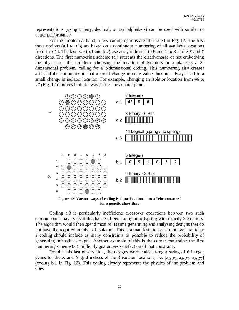
For the problem at hand, a few coding options are illustrated in Fig. 12. The firstthree options (a.1 to a.3) are based on a continuous numbering of all available locationsfrom 1 to 44. The last two (b.1 and b.2) use array indices 1 to 6 and 1 to 8 in the X and Ydirections. The first numbering scheme (a.) presents the disadvantage of not embodyingthe physics of the problem: choosing the location of isolators in a plane is a 2-dimensional problem, calling for a 2-dimensional coding. This numbering also createsartificial discontinuities in that a small change in code value does not always lead to asmall change in isolator location. For example, changing an isolator location from #6 to#7 (Fig. 12a) moves it all the way across the adapter plate.

2 3 4 5 6 7 81

2

3

4

5

6

1

9 10 11 ... .. .7

. .. ... 36 37 38

39 40 41 43 44

1 2 3 4 6

8

42

5

3 Binary - 6 Bits

44 Logical (spring / no spring)

6 Binary - 3 Bits

3 Integers

42 5 8

6 Integers

6 5 1 6 2 2

a.

b.

a.1

a.2

a.3

b.1

b.2

Figure 12 Various ways of coding isolator locations into a "chromosome"for a genetic algorithm.

Coding a.3 is particularly inefficient: crossover operations between two suchchromosomes have very little chance of generating an offspring with exactly 3 isolators.The algorithm would then spend most of its time generating and analyzing designs that donot have the required number of isolators. This is a manifestation of a more general idea:a coding should include as many constraints as possible to reduce the probability ofgenerating infeasible designs. Another example of this is the corner constraint: the firstnumbering scheme (a.) implicitly guarantees satisfaction of that constraint.

Despite this last observation, the designs were coded using a string of 6 integergenes for the X and Y grid indices of the 3 isolator locations, i.e. [x1, y1, x2, y2, x3, y3](coding b.1 in Fig. 12). This coding closely represents the physics of the problem anddoes

SAND96-116905/17/96

21

away with the need for back and forth conversions between integer and binaryrepresentations of the design variables. The alphabet (range) is 1..6 for x genes and 1..8for y genes.

6.2.3 Selection Operator

The selection operator is in charge of picking individuals for reproduction. It usesa biased roulette wheel where fitter individuals get larger portions of the wheel and havetherefore better chances of reproducing and transmitting their characteristics.

A ranking technique is used to assign portions on the roulette wheel: theprobability of selection of an individual is a function of its rank in the population - not itsfitness. This avoids the classical problem of the super-individual: if, early in the search, asingle design is - by chance - vastly superior to all others, a fitness-based selection wouldalmost always pick that super-individual and create a population of clones, leading tocomplete loss of genetic diversity. This does not happen with a rank-based selection rule.

SELECTProbability of Selection

Rank

SelectionPressure

Figure 13 Ranking selection operator.

Figure 13 illustrates the particular rule used in this application. The selectionpressure is defined as the ratio of the probability of selection of the best individual in thepopulation to that of the worst. High selection pressures push the search to fasterimprovement but also gives it less time to explore the design space. Again, a compromisemust be found. The selection pressure was set to 2 for this application.

6.2.4 Crossover Operator

Once two parents have been selected, their chromosomes undergo a crossoveroperation that generates an offspring chromosome. This GA uses a 2-point, non-averaging crossover illustrated in Fig. 14.

SAND96-116905/17/96

22

2 6 4 1 6 5

1 7 4 3 4 7

1 6 4 1 4 7

Parent 1

Parent 2

Child

2 randomcuttingpoints

Crossover

Figure 14 Non-averaging 2-point crossover operator.

The operator selects two random cutting points and creates a child chromosomeby assembling the inner and outer substrings from either parent. This operation is appliedwith a given probability Pc (typically large, 80 to 100%). When crossover is not applied,one of the 2 parent chromosomes (chosen at random) is simply cloned.

Notice that the child typically has some features from each parent but also somenew characteristics: the (1,6) location in the child’s chromosome in Fig. 14 for exampleresults from the combination of the x index from one parent and the y index from theother.

This crossover is called non-averaging because the cutting points are only allowedto fall between genes. In contrast, an averaging crossover (see for example [16]) generates cutting points that can fall anywhere within a gene. When thishappens, the child gene is computed as a weighted average of the parent genes. Theaveraging crossover was introduced to improve the GA’s behavior for problems withlarge alphabets: when a gene can take a large number of values, the initial population isunlikely to contain every possible value for that gene. Without averaging crossover, thegeneration of new values is left exclusively to the mutation. Artificially large anddisrupting mutation rates are then needed to maintain diversity. The averaging crossoveris also naturally indicated for problems with real-valued genes (which have an infinitealphabet).

For the current application, the alphabet is limited enough (1 to 6, or 1 to 8) that anon-averaging crossover may be sufficient, although further testing would clarify thispoint.

6.2.5 Mutation Operator

The mutation introduces random changes in the offspring chromosome resultingfrom the crossover operation. The role of the mutation is to prevent loss of geneticdiversity by introducing design features that may have never been present in thepopulation or may have been lost over time.

SAND96-116905/17/96

23

1 6 4 1 4 7

1 6 2 1 4 7

MutationPm

Random value

Figure 15 Mutation operator.

Mutation is applied with a small probability Pm to each gene in the chromosome.Figure 15 illustrates this process. When mutation occurs, the current value of the gene isreplaced by a random value, uniformly distributed in the range of that particular designvariable.

6.2.6 Constraint Enforcement

It is interesting to note that although most realistic engineering design problemsinvolve numerous constraints, little work has been done to investigate constraintenforcement strategies for genetic algorithms. One of four approaches is typically used:data structuring, direct elimination, repair operators, or penalty functions.

Data structuring consists of designing the coding in such a way that constraintsare automatically satisfied because infeasible designs can simply not be represented. Inour problem for example, the requirement to have exactly 3 isolators is automaticallysatisfied when using any coding scheme in Fig. 12, except a.3. Satisfaction of the cornerconstraint on the other hand is implicit with codings a.1 to a.3 but not with b.1 or b.2.Although data structuring is always the most efficient technique, it is only applicable forparticular types of constraints and is very problem-specific.

++

++

+

+

+ O

Figure 16 Design problem with disjoint feasible space.

In the direct elimination technique, each design resulting from selection,crossover, and mutation is examined for constraint satisfaction before it is included in thenew generation. If any constraint is violated, the offspring is eliminated and a replacementis created through new selection, crossover and mutation operations. This process isrepeated until a feasible design is found. This creates entirely feasible populations atevery generation, constraining the search exclusively within the feasible regions of thedesign space. In cases where the design space contains non-convex and/or disjointfeasible regions, this makes the search inefficient and unreliable. The reason is best

SAND96-116905/17/96

24

explained on a simple example. Figure 16 represents the design space of a 2-dimensionaldesign problem. The shaded areas represent infeasible regions and the arrow gives thegeneral direction of improvement of the objective function within the large feasible areaat the upper right of the figure. An initial feasible population for this problem is likely toreside entirely in the large feasible region of the design space. If direct elimination is

used, the GA will then converge to the local minimum within that area (• in Fig. 16),missing the global optimum (+). It is clear that convergence to the global optimum islikely only if the GA population is allowed to migrate through the infeasible “barrier” toreach the small feasible inclusion. Note that the feasible space does not have to be disjointfor this problem to occur: if the feasible space is non-convex, the GA may have tomigrate around a constraint barrier instead of short-cutting through it.

Another approach uses repair operators to “fix” infeasible designs beforeincorporating them in the new generation. Repair operators use some knowledge aboutthe problem to try and eliminate constraint violations through “small” modifications ofthe design. This approach is inherently problem-specific and is used mostly in researchalgorithms or GAs designed specifically for a particular class of problems. A simpleexample is shown in Fig. 17 for the corner constraint: an isolator located at a corner couldbe moved to one of the neighboring locations (one of three at random for example).

In less trivial cases however, it may be difficult to define design changes thateliminate given constraint violations. Also, in highly constrained problems, one cannotguarantee that ‘fixing’ a design for one constraint will not cause violation of another.Finally and most importantly, repair operators are problem-specific so they cannot beused in a general purpose optimization package like DAKOTA.

Figure 17 A simple repair operator for the corner constraint.

The fourth constraint enforcement technique uses penalty functions: in aminimization problem, each constraint violation produces an increase in the objectivefunction. Because penalty functions were originally introduced to enforce constraints inthe context of gradient-based optimization, classical definitions produce a smooth,differentiable transition from feasible to infeasible regions. This ‘blurs’ the boundaries ofthe feasible design space. A continuous optimization then converges to either slightlyinfeasible designs (when using exterior penalty functions[17]) or slightly conservativedesigns (with interior penalty functions). To avoid this and since there is no need toachieve continuity in the penalty functions with a zero order method like a GA, acombination of step and gradual penalties[18] (as shown in Fig. 18) will be used.

SAND96-116905/17/96

25

The steps prevent convergence to slightly infeasible designs while gradualpenalties maintain a logical hierarchy between designs with more or less severe constraintviolations. Gradual penalties are of course applied only to the quantifiable constraints(stability, compressive spring loads, and static spring deflections); Boolean constraints(corner constraints and isolator alignment) receive only a step.

Min

UnconstrainedObjective

Step Penalties

Gradual Penalties

T

+ ∑ steps

+ ∑ multipliers x (gi)2

i

i

Figure 18 Penalty function approach used in this application; the shadedarea is infeasible.

Just like in gradient-based optimization, adjusting penalty multipliers (and steps)is tricky. Too little penalty leads to infeasible designs, while too much makes the searchinefficient by restricting it to feasible regions. Unfortunately, because GAs are randomsearches and necessitate large numbers of function evaluations, trial and erroradjustments are impractical. A study by Richardson et al.[19] indicates that penaltiesshould be as small as possible, but large enough to prevent frequent convergence toinfeasible solutions and that using harsh penalties leads to poor convergence and/orpremature convergence to a super-individual. However, that study uses proportionalselection (probability of selection based on objective function value); its conclusions donot hold when using a ranking selection rule. In fact, it appears from limitedexperimentation with this problem that the reliability of the search is best with harshpenalties associated with a weak selection pressure (the selection pressure was set to 2,see Section 6.2.3). Note again that because of the random character of GA’s and theinteraction between multiple parameters (probabilities of mutation and crossover,population size and number of generations per search, penalty multipliers and steps, etc.),statistically significant conclusions can be reached only through extensive (andexpensive) experimentation.

6.3 Rounding of Continuous Optimum

In this approach (Fig. 19), all design variables are temporarily viewed ascontinuous and classical gradient-based techniques are used to solve the optimizationproblem. The resulting optimal design is infeasible and its parameters must be “rounded”to discrete values.

SAND96-116905/17/96

26

AnalyseFEASIBLE ? OPTIMAL ?

Discrete Design(s)

Solve Optimization Problem incontinuous design space

x ∈ [1...6] and y ∈ [1...8]

“Round” to close discrete solution

Continuous Optimum

Figure 19 Using continuous approximation followed by rounding tonearby discrete solution.

The appeal of this technique is the much smaller number of function evaluationstypically needed to achieve convergence with a gradient based technique than with arandom search method. However, the rounding operation can make the design infeasibleor suboptimal. Also, many different designs can be defined by rounding up or down thevarious design variables. To increase the chances of optimality, all these “directneighbors” must be considered and analyzed. When the number of discrete designvariables is large, this may require a substantial number of additional function evaluations(2n if n is the number of design variables) so that the computational advantage may belost. These points are further discussed in Section 7.2.

7. Optimization Results

7.1 Genetic Algorithm and Random Search

The GA in DAKOTA provides a number of options and adjustments. Thefollowing choices were made for this application:

• population of 10 individuals (designs). The initial population is random. With 10individuals, the probability of representation of any gene value (1 to 6, or 1 to 8) at anygene location is close to 1, which should ensure good performance with a non-averagingcrossover

• probability of crossover: 0.80• probability of mutation: 0.10. This gives a 60 to 80% probability for any

offspring to be affected by mutation.• elitist strategy always clones the best individual of the current generation into

the next generation. This guarantees that the best found design is never lost in futuregenerations.

• number of generations : 15 (experiments with smaller numbers of generationsdid not achieve sufficient reliability)

• moderate selection pressure: the probability of selection of the best individual istwice that of the worst (i.e. selection pressure=2).

SAND96-116905/17/96

27

Penalty multipliers and steps were adjusted somewhat arbitrarily. Limited trial anderror experimentation was performed and lead to the following values:

• corner constraints g1, g2, g3: step = 5.0.• alignment constraint g4: step = 20.• stability constraint g5: step = 2, multiplier = 20.• compression constraints g6, g7, g8: step = 5, multiplier = 0.05.• static deflection constraints g9, g10, g11: step = 5, multiplier = 200.

0

2

4

6

8

10Random Search GA Search

10 Runs - 105 Function evaluations each

T[µin/sec/lb]

Figure 20 Comparison of genetic algorithm and random search resultsusing the same number of function evaluations (105). Designs shown are

the best found for each run.

The design space for this problem is relatively small: 6×8 locations for each of 3isolators gives 483 ≅ 110,000. With 15 generations of 10 individuals, each searchevaluates up to 150 designs, or 0.14% of the design space. Note that because this GAkeeps track of previously analyzed designs, the actual number of function evaluationsaverages around 105 per search (0.1%). To get an idea of the reliability of the search, aseries of 10 runs were performed and the results are compared to a series of 10 randomsearches. The number of designs in the random search is set to 105 so the computationalexpense is the same as in the GA. Typical results are shown in Fig. 20. The figure showsonly the best design found in each run of the GA or the random search. The randomsearches generate some good designs and many mediocre ones. In contrast, all 10 designsobtained from the GA represent significant improvements from the baseline case.However, the GA occasionally "converges" to a relatively poor design (T=3.23 in Fig.20). This implies that more reliable results can be obtained by running a small number ofshort searches: if the probability that the best found design is "poor" is 0.1 for a one run,then it is only 0.01 for the best of 2 runs, 0.001 for the best of 3, etc. Because GA’s aremost efficient in the initial phases of the search and further "convergence" is usually slow,this approach is often preferable to running a single longer search[18].

It is interesting to note that the classical argument that a GA provides a choicebetween several good designs in the final population does not hold in this application.Instead, final populations typically contain only one or two feasible design(s). In fact, allgenerations in the search are composed mostly of infeasible designs. This shows that the

SAND96-116905/17/96

28

search is taking place primarily in infeasible regions of the design space. Under theseconditions, it is particularly crucial to allow the search to migrate through infeasibleregions. This may also explain why a weak selection pressure provides better results withthis problem.

21.22

0.30 0.34 0.41

0.41 0.47 0.49

0.59 0.59 0.67

Baseline

Figure 21 GA optimized designs and their transmissibilities at 50 Hz (inPin/sec/lb), compared to baseline configuration.

Several sets of 10 runs each were performed in the course of this study. Nine ofthe best designs obtained form those runs are shown in Fig. 21 and compared to thebaseline design. The transmissibilities at 50 Hz are also listed in the figure. Clearly, all 9optimized designs represent very significant improvements from the baseline case:transmissibilities are reduced by factors 32 to 70 compared to baseline.

Note also that the 9 optimized designs do not have any apparent similaritiesalthough they provide very similar performances. This indicates the existence of multiplelocal optima for this problem.

Figure 22 shows frequency response functions (FRF’s) for all designs of Fig. 21.They show that the GA is seeking out an anti-resonance condition in the vicinity of 50Hz. The fact that the anti-resonances “miss” the 50 Hz target is due to the discrete isolatorlocations. In fact, the continuous optimum of the next section places the antiresonancealmost exactly at 50Hz, achieving a transmissibility of 0.2 µin/sec/lb. Another importantobservation is that there is significant broad-band improvement in the transmissibilities ofthe optimized designs compared to the baseline design. That is, the improvement is notconfined only to the 50 Hz target frequency. This is an especially important observationsince it indicates that performance is not seriously degraded for off-nominal excitationinputs and more sophisticated objective function formulations minimizing broad bandtransmissibility are probably unnecessary.

SAND96-116905/17/96

29

T(in/sec/lb)

Frequency (Hz)

20 40 60 80 100010-8

10-6

10-4

10-2

10 0

Baseline Design

Optimized designs

a 30 dB

Figure 22 Transmissibility curves of optimized designs compared tobaseline configuration (model predictions).

7.2 Rounding of Continuous Optimum

DOT’s[20] modified method of feasible directions (accessible through DAKOTA)was used to solve the constrained, non-linear continuous problem. A continuous solution(+ in Fig. 23) was found at (2.22, 1.56, 2.49, 4.94, 4.29, 3.79) with a transmissibilityT=0.20 µin/sec/lb at 50 Hz. Rounding to the closest discrete solution (O in Fig. 23) leadsto (2,2,2,5,4,4), which is infeasible (violates the 4Hz stability limit). If we consider allimmediate neighbors of the continuous solution (all combinations of O and O in Fig. 23),we find that out of the 64 designs, only 12 are feasible and the best of these (2,1,3,5,5,3)gives T=3.67 µin/sec-lb. This transmissibility is 22 times higher than that of the best GAsolution (T=0.30) and only 6 times better than the baseline configuration (T=21.22).

Continuous optimum

Closest discrete design

Immediate neighbors

(2.22, 1.56, 2.49, 4.94, 4.29, 3.79) . . . . .

(2, 2, 2, 5, 4, 4) . . . . . . . . . . . . . . . . . . .

64 designs: - 52 infeasible

- 12 feasible . . . . . . . .

T = 0.20

infeasible

best T = 3.67

Figure 23 Results from continuous optimization and rounding.

SAND96-116905/17/96

30

Continuous approximation leads - for this problem - to many infeasible designsand a few sub-optimal solutions. Although this particular application is particularlydifficult for continuous approximation (because of the low density of feasible designs andthe very coarse discrete grid), two general observations can be made:• continuous solutions for constrained problems tend to make one or more constraint(s)

active. Rounding those solutions is likely to produce violations of the activeconstraint(s).

• optimal regions in the continuous problem may not contain any discrete solution. Thediscrete optimum may then be very different from the continuous one. This isparticularly true when the discrete grid is coarse compared to the shortest wavelengthsin the objective function response surface.

Discreteoptimum

ContinuousOptimum

closestdiscrete

best neighbor

Objective

Design Variable

Constraint boundary

Figure 24 Rounding a continuous optimum to neighboring discretesolutions.

Figure 24 illustrates these points for a one-dimensional constrained problem. Thecurve represents the variation of the objective function in a continuous design space.Dotted vertical lines show the discrete grid of the actual problem and the solid line givesthe constraint boundary. If appropriate starting points are used for the continuousoptimization, the global continuous optimum will be found at + (the global optimum inthe continuous sense). This design makes the constraint active. The closest discretesolution (O) violates the constraint while the other direct neighbor solution is far fromoptimal. The discrete optimum (shown by the arrow in the figure) does not “resemble” itscontinuous counterpart.

7.3 A Look at the Design Space

To understand the behavior of the optimizers, it is interesting to take a look at thetopography of the design space. In particular, the relative sizes of feasible and infeasibleregions and the rates of variation of the objective function are critical factors thatinfluence the efficiency of optimization algorithms.

To answer the first question, a Monte Carlo simulation was performed in which1000 random combinations of isolator locations were selected at random and theirobjective function and constraints were calculated. The results show that only 12.7% ofthe designs are feasible, indicating a heavily constrained problem. The mean objectivefunction value for the feasible designs is equal to T=21.1 µin/sec/lb. As mentioned

SAND96-116905/17/96

31

earlier, this value is almost exactly equal to the transmissibility of the baselineconfiguration which can therefore be considered representative (in other words, thebaseline design is not exceptionally poor). Also, the distribution of isolator locationsamong the feasible designs does not depart significantly from uniform (except for the 4corners which are never used). This indicates that “good” designs do not tend to useparticular locations on the grid. It is only the combination of 3 locations that determines adesign’s feasibility.

T = 0.47

0

20

40

60

80T

0

20

40

T

unconstrained constrained

Figure 25 Two-dimensional cut through the design space obtained bymoving one isolator in both directions; for clarity, the constrained

objective plot only shows step penalties.

The 6-dimensional design space of this problem cannot be visualized easily.However, 2-dimensional cuts can be obtained by fixing the locations of 2 of the isolatorsand moving the third one in the X and Y directions. The GA design (1,6,2,8,5,3) withT=0.47 from Fig. 21 is used as a starting point. The locations of the two isolators near thetop right corner (1,6) and (2,8) are fixed while the third one is moved across the plane,ignoring the grid. This generates the 2-dimensional cut (1,6,2,8,x,y with x,y∈ℜ ) in thedesign space. Figure 25 shows both unconstrained and constrained (steps penalties only)response surfaces. Note that —in the continuous sense— there is not a unique optimumbut rather a infinity of locations (the dotted curve in Fig. 26) for the third isolator thatachieve a small transmissibility (0.2) by designing an anti-resonance at the exact locationof the pickup point.

SAND96-116905/17/96

32

13.15.4

12.3

12.0

0.47

X

Y

1

2

3

4

5

6

1 2 3 4 5 6 7 8

alignmentstatic deflection

stabilitycompressive load

com

pres

sive

load

Figure 26 Design space cross section showing unconstrained objective,discrete grid, contour lines, constraint boundaries, feasible domain

(shaded), and feasible discrete designs with their transmissibilities; the +shows the discrete optimum.

The same cut is represented in Fig. 26: here, contour lines of the unconstrainedobjective function are plotted together with constraint boundaries. Discrete isolatorlocations are shown with small circles. Note the small size of the feasible domain(shaded). Only 5 discrete designs are contained in that area; their transmissibilities T at 50Hz are listed in the figure.

Note also that the location (5,3) found by the GA for the 3rd isolator is the discreteoptimum (+) for the given locations of the other 2 isolators. It was found that this is thecase of almost all locations used in the designs of Fig. 21, which indicates that theycorrespond to various local optima and confirms the strong multi-modality of thisproblem.

The small size of the feasible regions (12.7% of design space) and the coarsediscrete grid create small feasible “pockets”, each containing few discrete solutions. Thisexplains the difficulties encountered in the GA searches. The search has to take placealmost entirely in the infeasible design space because the number of designs in each“pocket” is too small to allow efficient exploitation by the GA. This also leads to mostlyinfeasible populations so that each run provides only one or two feasible design(s).

Also, there is very strong coupling between design variables: it is only specificcombinations of 3 locations that enable the small transmissibilities of Fig. 21. In Fig. 26for example, the locations of the 2 fixed isolators selected by the GA are such that there isa feasible discrete location almost exactly on the anti-resonance line (dotted curve in thefigure).

8. Experimental Results

The baseline configuration and all 9 optimized designs of Fig. 21 were tested inthe laboratory. Because of the limited load capability of the shaker, the very large inertiaof the seismic base, and the effectiveness of the optimized isolation systems, residual

SAND96-116905/17/96

33

velocities proved difficult to measure because of marginal signal to noise ratio and thepresence of acoustic disturbances. To “clean up” the velocity signal, about 200 samplestriggered on the 50Hz sinusoidal excitation signal were averaged in the time domain. Theresults are shown in Fig. 27 and compared to analytical predictions. The figure also showspredicted ranges of transmissibilities with ±5% scatter in the spring stiffnesses. Thoseranges were obtained from Monte Carlo simulations using uniform distributions of springstiffnesses with ±5% variations; the stiffnesses of the 3 spring isolators were variedindependently from each other.

T(µin/sec/lb)

0

5

10

15

20

25

experimental

nominal

+/- 5% spring stiffness variations

Figure 27 Experimental transmissibilities at 50 Hz of baseline andoptimized designs, compared to analytical predictions.

The analytical-experimental agreement is qualitatively excellent: the dramaticimprovement in performance achieved through optimization as predicted by the analysisis confirmed by the experiment. All 9 optimized designs perform between 7 and 46 timesbetter than the baseline configuration (predicted ratios were between 32 and 70).

9. Conclusions

9.1 Optimum Isolation System Design

Our results confirm that in cases where vibration isolation must be provided atspecific points/directions on a device and sufficient information is available about thedisturbances, very significant improvements in performance can be achieved by explicitlyoptimizing the locations of the isolators. In the particular application, the performance ofthe optimized designs was predicted between 32 to 70 times better than that of a baselineconfiguration. Those improvements were also observed in the laboratory, withperformance ratios between 7 and 46. It was also shown that, even though theoptimization was formulated to “target” transmissibility at a single frequency, significantbroad-band improvement was obtained in the optimized designs compared to the baselineconfiguration.

SAND96-116905/17/96

34

9.2 Discrete Optimization

• Applying constraints through penalty functions in a GA problem is a delicateoperation. A balance must be achieved between the desire to obtain a feasible final designand the need to allow the search to cross infeasible regions of the design space.Surprisingly little research has been devoted to this aspect. One reason is that, in researchGA’s, problem-specific repair operators are often introduced to enforce constraints. Thisapproach is more efficient but is highly application-specific and cannot be included ingeneral purpose codes like DAKOTA.

• The combination of multi-modality, large number of constraints, and limiteddesign options (coarse discrete grid in this case) makes the problem difficult to handle,even for a zero-order random search technique like the GA.

• The classical argument that a GA provides multiple design alternatives in itsfinal population does not hold in heavily constrained discrete problems with small designspaces. Instead, each run provides only one or two acceptable designs.

• Multiple design options and improved reliability of the search can be obtainedby running a few short searches, rather than a single long search.

• Continuous optimization followed by rounding to neighboring discrete solutionsdoes not generally lead to an optimal design. For problems with coarse discrete grids,heavily constrained design space, and rapidly varying objective function, this approachleads to few, relatively poor feasible designs.

These observations have uncovered the need for further research if discreteoptimization is to become a practical, easy to implement technique for use in real lifedesign problems. In particular, techniques for efficient implementation of multipleconstraints in genetic algorithm optimization need further exploration and development.

10. References

1. Crede, C. E., Vibration and Shock Isolation, J. Wiley & Sons, ed., New York, NY,1951.

2. Ashrafiuon, H., “Design Optimization of Aircraft Engine-Mount Systems,” Journal of

Vibration and Acoustics, ASME, Vol. 115, October 1993, pp.463-467. 3. Hart, W. E., Evolutionary Pattern Search Algorithms, Sandia Report SAND95-2293,

September 1995. 4. Eldred, M. S., Outka, D. E., Bohnhoff, W. J., Witkowski, W. R., Romero, V. J.,

Ponslet, E. R., and Chen, K. S., “Optimization of Complex Mechanics Simulationswith Object-Oriented Software Design,” Computer Modeling and Simulation inEngineering, to appear.

5. Newport Corp., Irvine, CA. 6. Associated Springs-Raymond (BARNES Group Inc.), Cerritos, CA 90703.

SAND96-116905/17/96

35

7. Firestone Industrial Products Company, Noblesville, IN. 8. Endevco Corp., San Juan Capistrano, CA. 9. PCB Piezotronics Inc., Depew, NY. 10. Wilcoxon Research Inc., Gaithersburg, MD. 11. MB Dynamics Inc., Cleveland, OH. 12. Pro-Engineer, Users Manual, Parametric Technology Group, Waltham, MA. 13. Meza, J. C., OPT++: An Object-Oriented Class Library for Nonlinear Optimization,

Sandia Report SAND94-8225, March 1994. 14. MATLAB Users Manual, The MathWorks, Inc., Natick, MA. 15. Davis, L., Handbook of Genetic Algorithms, Van Nostrand Reinhold Pub., 1991. 16. Ponslet, E., Haftka, R. T., and Cudney, H. H., “Optimal Placement of Tuning Masses

on Truss Structures by Genetic Algorithms,” Proceedings of the 34th AIAA/ ASME/ASCE/ AHS /ASC Structures, Structural Dynamics, and Materials Conference, April19-22, 1993, La Jolla, CA, part 4, pp. 2448-2457 (AIAA paper 93-1586).

17. Haftka, R. T., Gurdal, Z., and Kamat, M. P., Elements of Structural Optimization,

second revised edition, Kluwer Academic Pub., Dordrecht, The Netherlands, 1990. 18. Leriche, R., Composite Structures Optimization by Genetic Algorithms, Ph.D.

Dissertation, Virginia Tech, Blacksburg, VA, 1994. 19. Richardson, J. T., Palmer, M. R., Liepins, G., and Hilliard, M., "Some Guidelines for

Genetic Algorithms with Penalty Functions," Proceedings of the Third InternationalConference on Genetic Algorithms, George Mason Univ., Morgan Kaufmann Pub.,June 4-7, 1989, pp. 191-197.

20. DOT Users Manual, Vanderplaats Research and Development, Inc., Version 4.20,

Colorado Springs, CO, 1995.