coupling wind farm with nuclear power plant a thesis
TRANSCRIPT

Ain Shams University
Faculty of Engineering
Electrical Power and Machines Engineering Department
Coupling Wind Farm with Nuclear Power Plant
A Thesis
Submitted in partial fulfillment of the requirements of the degree of
Master of Science in Electrical Engineering
Submitted by
Mohamed Kareem Abdel Rahman Al-Ashery
B.Sc. of Electrical Engineering
Electrical Power and Machines Engineering
Ain Shams University, 2008
Supervised by:
Prof. Dr. Mohamad Abd Al Rahim Badr
Dr. Walid El-Khattam
Dr. Moustafa Saleh El Koliel
Cairo, 2014


i
Ain Shams University
Faculty of Engineering
Electrical Power and Machines Engineering Department
Coupling Wind Farm with Nuclear Power Plant
A Master of Science thesis Submitted by
Mohamed Kareem Abdel Rahman Al-Ashery
EXAMINERS’ COMMITTEE
Name Signature
Prof. Essam El-Din Mohamed Abou-El-Zahab
Cairo University, Faculty of Engineering,
Electrical Power and Machines Engineering Dept.
…………
Prof. Almoataz Youssef Abdelaziz Mohammed
Ain Shams University, Faculty of Engineering,
Electrical Power and Machines Engineering Dept.
…………
Prof. Mohamad Abd Al Rahim Badr
Future University,
Dean, Faculty of Engineering and Technology
…………
Dr. Walid Ali Seif El-Eslam El-Khattam
Ain Shams University, Faculty of Engineering,
Electrical Power and Machines Engineering Dept.
…………
Date: / / 2014

ii
Researcher Data
Name: Mohamed Kareem Abdel Rahman Al-Ashery
Date of Birth: 25/6/1986
Place of Birth: Saudi Arabia
Academic Degree: B.Sc. in Electrical Engineering
Field of specialization: Electrical Power and Machines Engineering
University issued the degree: Ain Shams University
Date of issued degree: 2008
Current job: Research assistant, Egyptian Atomic Energy Authority

iii
Statement
This dissertation is submitted as partial fulfillment of Master of Science in
Electrical Engineering, Faculty of Engineering, Ain Shams University.
The author carried out the work included in this thesis, and no part of it has been
submitted for a degree or qualification at any other scientific entity.
Student Name: Mohamed Kareem Abdel Rahman Al-Ashery
Signature:
Date: 22 / 7 / 2014

iv
Acknowledgments
الحمد لله رب العالمين
All praise is due to ALLAH, the Lord of the Worlds, Most Gracious, Most
Merciful; Who taught man that which he knew not.
I would like to thank all the people who contributed in some way to the work
described in this thesis. First and foremost, I wish to express my gratitude to my
supervisors, Prof. Dr. Moh Abd El Rehim Badr, Dr. Walid El-Khattam, and Dr.
Moustafa El Koliel for their exceptional guidance, encouragement, insightful thoughts
and useful discussions. I would like to thank Prof. Badr for accepting to be my
supervisor in this project. My sincere appreciation goes to Dr. Walid for all I have
learned from him and for his continuous help and support in all stages of this thesis. I
would also like to thank him for being an open person to ideas, and for encouraging and
helping me to shape my interest and ideas. I would like to thank Dr. Moustafa for his
valuable advices that help me not only in my thesis, but also in my life.
I would like to thank my colleagues and friends for their support and help. My
sincere thanks go to my colleagues at the Egyptian Atomic Energy Authority. Special
thanks to Ahmed Sallam, my colleague at Egypt Era, for useful discussions during my
thesis. I would like to acknowledge my friends at Nuclear Power Plant Authority,
Mohamed Essa, Mohamed Ramadan, and Mostafa Fouad for their valuable technical
discussions.
Last but not least, I would like to thank my parents. Their unlimited care, their
patience and love have always guided my through my whole life. I wish ALLAH help
me reward them only part of what they did for me.
Moh Kareem Al-Ashery,
Cairo, Egypt,
2014

v
Abstract
Mohamed Kareem Abdel-Rahman Al-Ashery, Coupling Wind farm with Nuclear
Power Plant, Master of Science dissertation, Ain Shams University, 2014.
Climate change has been identified as one of the greatest challenges facing nations,
governments, businesses and citizens of the globe. The threats of climate change
demand an increase in the share of renewable energy from the total of energy
generation. Meanwhile, there are tremendous efforts to decrease the reliance on fossil
fuel energies which opens the venue for increasing the usage of alternative resources
such as nuclear energy. Many countries (e.g. Egypt) are planning to meet increasing
electricity demands by increasing both renewable (especially wind energy) and nuclear
energies contributions in electricity generation.
In the planning phase of siting both new Wind Farms (WFs) and Nuclear Power
Plants (NPPs), many benefits and challenges exist. An important aspect taken into
consideration during the NPP siting is the existence of ultimate heat sink which is sea
water in most cases. That is why most NPPs are sited on sea coasts. On the other hand,
during WF siting, the main influential aspect is the existence of good wind resources.
Many coastal areas around the world fulfill this requirement for WF siting. Coupling
both NPPs and WFs in one site or nearby has many benefits and obstacles as well. In
this thesis, based on international experience and literature reviews, the benefits and
obstacles of this coupling/adjacency are studied and evaluated. Various case studies are
carried out to verify the coupling/adjacency concept.
Index Terms – Coupling NPP and WF, Reliability and Availability using Markov
Process, WFs’ grid requirements WFs’ Capacity Credit and geographical distribution.

vi
Summary
This thesis studies and evaluates the benefits and obstacles of coupling of Wind
Farms (WFs) with Nuclear Power Plants (NPPs). The dissertation is divided into five
chapters organized as follows:
Chapter One: It is an introduction to the idea of coupling of WF with NPP.
Motivation of the idea and the thesis outline are discussed.
Chapter Two: This chapter presents the literature survey, and the characteristics of
the site that can accommodate both NPP and WF are illustrated. It also evaluates
different sites in Egypt that can accommodate coupling. Finally, advantages and
disadvantages of coupling of WFs with NPPs are explained.
Chapter Three: It illustrates the benefits of connecting WF and NPP to the same
point of the grid. Two case studies are conducted to verify two main benefits of this
adjacency, which are the impact of high short circuit power level on the voltage quality
aspects of WF, and increasing reliability and availability of NPP Emergency Power
Systems (EPSs) by the on-site WF.
Chapter Four: The benefit of helping in geographical distribution of WFs in the grid
is discussed in details. A case study is conducted to illustrate the smoothing effect of
WFs geographical distribution in the Egyptian grid. After that, wind energy capacity
credit assessment is done considering the case in Egypt. Finally, Strategic plan for the
coupling in Egypt is illustrated, considering the coordination between WFs and NPPs
new installations.
Finally, the thesis ends by extracting conclusions and stating future work that might
be done based on this work.
vii
Contents
LIST OF FIGURES .......................................................................................................... X
LIST OF SYMBOLS .................................................................................................... XIII
LIST OF ABBREVIATIONS ..................................................................................... XVI
CHAPTER 1: INTRODUCTION ..................................................................................... 1
1.1 ELECTRICITY IN EGYPT: CURRENT AND FUTURE ...................................................... 1
1.2 THESIS MOTIVATION ............................................................................................... 2
1.3 THESIS OUTLINE ...................................................................................................... 2
CHAPTER 2: LITERATURE SURVEY ....................................................................... 4
2.1 PREVIOUS WORK ..................................................................................................... 4
2.2 SITE SELECTION FOR COUPLING OF WF WITH NPP .................................................. 5
2.2.1 NPP site selection ............................................................................................ 5
2.2.2 WF Site Selection ............................................................................................ 7
2.2.3 Site selection for coupling ............................................................................... 8
2.2.4 Proposed sites for coupling in Egypt ............................................................... 9
2.3 ADVANTAGES OF COUPLING OF WF WITH NPP ..................................................... 12
2.3.1 Good use of the low population density areas around NPPs ......................... 12
2.3.2 Existence of connection to grid ..................................................................... 13
2.3.3 Existence of main facilities required for power plant construction, operation
and maintenance ........................................................................................... 14
2.3.4 Other benefits of coupling ............................................................................. 15
2.4 DISADVANTAGES OF COUPLING OF WFS WITH NPPS ............................................ 15
2.4.1 Technical problems which can be overcome by proper solutions ................. 15
2.4.1.1 High short circuit power level of PCC and WF’s protection switchgear 15
2.4.1.2 Noise from WTs ..................................................................................... 16
2.4.1.3 Shadow flicker and blade glint ............................................................... 16
2.4.1.4 Interference of WTs with the communication systems of NPP.............. 17
2.4.1.5 Wind energy power quality aspects and its impact on NPP ................... 17
2.4.1.6 Lower energy production from WF ........................................................ 18

viii
2.4.2 Accident hazards from WF ............................................................................ 18
2.4.2.1 Fire hazards............................................................................................. 19
2.4.2.2 Unique industrial risks ............................................................................ 19
2.4.2.3 Aviation operations hazards (Aircraft safety) ........................................ 19
CHAPTER 3: CONNECTING WF AND NPP TO THE SAME POINT IN THE GRID
........................................................................................................................................ 21
3.1 BENEFITS OF COUPLING ON THE GRID INTEGRATION ISSUES OF WF ....................... 21
3.1.1 Voltage quality at the coupling point of WF ................................................. 21
3.1.1.1 Main requirement for WF grid integration ............................................. 22
3.1.1.2 Fulfillment of the main requirement for WF grid integration using
Coupling ................................................................................................. 24
3.1.1.3 Case study illustrating the effect of short circuit capacity on the voltage
quality aspects of WF ............................................................................. 25
3.1.2 Active power / frequency control capability ................................................. 31
3.1.2.1 Benefits of coupling on the active power / frequency control capability of
the WF .................................................................................................... 31
3.1.3 Reactive power / voltage control capability .................................................. 32
3.1.3.1 Benefits of coupling on reactive power / voltage control capability of WF
................................................................................................................ 33
3.2 INCREASING RELIABILITY AND AVAILABILITY OF NPP EPSS BY THE ON-SITE WF 34
3.2.1 NPP electrical system .................................................................................... 35
3.2.2 The benefit of adjacency of WF & NPP on the NPP electrical system ......... 37
3.2.3 Using MARKOV Process to illustrate EPS’s Reliability and Availability
enhancement using on-site WF ..................................................................... 38
3.2.3.1 Calculation of reliability and availability for Emergency Diesel
Generators (DGs) set .............................................................................. 42
3.2.3.2 Calculation of reliability and availability for WTs set ........................... 43
3.2.3.3 Enhancement achieved in reliability and availability by adding WTs to
EPSs of NPP (Wind – Diesel system) .................................................... 47
CHAPTER 4: ASPECTS RELATED TO ADJACENCY BETWEEN WF AND NPP 53
4.1 GEOGRAPHICAL DISTRIBUTION OF WFS IN THE GRID ............................................. 53

ix
4.1.1 Case study for the effect of WFs geographical distribution on the aggregation
of wind power production in Egypt .............................................................. 55
4.2 IMPACT OF GEOGRAPHICAL DISTRIBUTION ON THE CAPACITY CREDIT OF WIND
ENERGY ................................................................................................................. 64
4.3 WIND ENERGY CAPACITY CREDIT ASSESSMENT (CASE STUDY IN EGYPT) ............. 64
4.4 STRATEGIC PLANNING (CASE STUDY IN EGYPT) .................................................... 68
4.5 LEVELIZED COST OF ENERGY (LCOE) .................................................................. 69
4.5.1 Comparing LCOE for Cases A & B and Scenarios I, II, & III ...................... 75
CHAPTER 5 ................................................................................................................... 79
CONCLUSIONS AND FUTURE WORK ..................................................................... 79
REFERENCES ............................................................................................................... 81

x
List of Figures
Figure 2.1: Geographical locations for sites under evaluation to accommodate NPP in
Egypt ........................................................................................................... 10
Figure 2.2: Wind Atlas of Egypt .................................................................................... 10
Figure 3.1: Classification of different power quality phenomena .................................. 22
Figure 3.2: Equivalent circuit ......................................................................................... 23
Figure 3.3: Reactive power control requirement as a function of grid voltage (EON Netz
GmbH) ........................................................................................................ 33
Figure 3.4: Simplified single line diagram of the NPP electrical system ....................... 36
Figure 3.5: A simplified single line diagram of EPSs block .......................................... 37
Figure 3.6: Markov graph for single OGU ..................................................................... 40
Figure 3.7: WT generator power curve .......................................................................... 40
Figure 3.8: Markov graph for single WT ....................................................................... 40
Figure 3.9: Markov graph for two identical DGs ........................................................... 42
Figure 3.10: Markov graph for two identical WTs working in parallel ......................... 44
Figure 3.11: Two systems A and B connected in parallel .............................................. 48
Figure 3.12: Availability versus time (hours) ................................................................. 50
Figure 3.13: Reliability versus time (hours) ................................................................... 51
Figure 3.14: Availability versus time (hours) for Wind-Diesel System and DGs set, with
minimum production of 20 MW from WF ................................................. 52
Figure 3.15: Reliability versus time (hours) for Wind-Diesel System and DGs set, with
minimum production of 20 MW from WF ................................................. 52
Figure 4.1: An example of large-scale wind power production in Denmark, January
2000 ............................................................................................................. 53
Figure 4.2: Impact of geographical distribution and additional WTs on aggregated
power production ........................................................................................ 54
Figure 4.3: Annual generation in percentage of available capacity ............................... 61
Figure 4.4: Duration curves for the generation in percentage of available capacity cases
..................................................................................................................... 62
Figure 4.5: Duration curves of monthly variations, as a percentage of the installed
capacity ....................................................................................................... 63

xi
Figure 4.6: Flow Chart for Capacity Credit calculations using the PJM method ........... 66
Figure 4.7: Capacity Credit (%) for El Zayat Site for WTs used in various scenarios
versus the times of peak loads ..................................................................... 67
Figure 4.8: Flow chart for the procedure of calculating LCOE for any power plant ..... 71
Figure 4.9: Relation between Variable O & M Costs and LCOE with other factors
equals to that of the median case in Table 4.7 ............................................ 73
Figure 4.10: Relation between Discount Rate and LCOE with other factors equals to
that of the median case in Table 4.7 ............................................................ 73
Figure 4.11: Relation between Capacity Factor and LCOE with other factors equals to
that of the median case in Table 4.7 ............................................................ 74
Figure 4.12: Relation between Capital Cost and LCOE with other factors equals to that
of the median case in Table 4.7 ................................................................... 74
Figure 4.13: Scenario I: LCOE for cases A & B versus capital cost reduction (%) due to
coupling, with operation & maintenance cost reduction (%) as a parameter
..................................................................................................................... 77
Figure 4.14: Scenario II: LCOE for cases A & B versus capital cost reduction (%) due
to coupling, with operation & maintenance cost reduction (%) as a
parameter ..................................................................................................... 77
Figure 4.15: Scenario III: LCOE for cases A & B versus capital cost reduction (%) due
to coupling, with operation & maintenance cost reduction (%) as a
parameter ..................................................................................................... 78

xii
List of Tables
Table 2.1: Average wind speeds in the selected sites at 50 m/s a.g.l. ............................ 11
Table 2.2: Guide to the Amount of Power Carried Through Power Networks .............. 14
Table 3.1: Data of the proposed sites ............................................................................. 28
Table 3.2: Data of the used Type A WT......................................................................... 28
Table 3.3: Data of the used Type D WT......................................................................... 29
Table 3.4: Scenarios under study .................................................................................... 29
Table 3.5: Calculation results for voltage quality aspects for all scenarios ................... 30
Table 3.6: Cost implications of WT power factor capability of 0.9 ............................... 33
Table 3.7: Reliability and Availability data for DGs used in NPP ................................. 43
Table 3.8: Conditions associated with each state in Figure 3.10 .................................... 45
Table 3.9: Data for the used WTs and there site (El Dabaa) .......................................... 47
Table 4.1: Geographical coordination of the three sites ................................................. 55
Table 4.2: Monthly mean wind speeds (m/s), at a height 24.5 m a.g.l. for El Galala .... 56
Table 4.3: Monthly mean wind speeds (m/s), at a height 24.5 m a.g.l. for Zafarana ..... 57
Table 4.4: Range of monthly variations, as a percentage of the installed capacity ....... 64
Table 4.5: Capacity Credit (%) for El Zayat Site for WTs used in various scenarios
versus the times of peak loads ...................................................................... 67
Table 4.6: NPP Timing and Sizing (MW) Selection Based on WFs MW Installations . 69
Table 4.7: Data for electricity generation costs from on shore WFs around the world .. 72
Table 4.8: Aspects related to coupling and their projected increase/decrease in costs of
electricity generation .................................................................................... 78

xiii
List of Symbols
%PWF (Vt) The power generation from WF in percentage of installed capacity
A Transition rate matrix
C Scale parameter of the 2-parameter Weibull distribution
c(Ψk, Va) Flicker coefficient
dso Switching operations voltage change of the grid at PCC (normalised
to nominal voltage)
dss Steady state voltage change of the grid at PCC (normalised to
nominal voltage);
F Set of failure states of the system
f(v) Probability density function of the 2-parameter Weibull distribution
of wind speed (v)
K Shape parameter of the 2-parameter Weibull distribution
kf(Ψk) Flicker step factor;
ku(Ψk) Voltage change factor
N Number of states
n Reading number;
N120 Number of switchings within a 2 hours period
Nr Total number of readings for each case (24*12=288)
NWT Number of WTs in the WF
Ø Phase angle between voltage and current
Ø06 Probability that wind speed is in the region of S0 (Vi <V< Vr) and
decreases to be in the region of state S6 (V< Vi)
P(Vt) Power output of the WT at wind speed (Vt)
P0(t) Probability function in time of state S0
PE Equipment installed capacity (MW)
Pi(t) Probability of system to be in state (i) function in time
Plt Flicker distortion
Pn Output power (% installed capacity) according to reading number (n)
Pr Rated power output of the WT
Pr (Vi<V<Vr ) Probability of wind speed to be above (Vi) and below (Vr)
xiv
PWF(Vt) Electrical power generated by WF (MW)
QA Unreliability or unavailability of system A
Qp Unreliability or unavailability of the parallel system
RA Reliability or availability of the system A
RL Short circuit resistance of the grid
Rp Reliability or availability of the parallel system
RSC Short Circuit Ratio
S Set of success states of the system
S60 Apparent power at the 1-min. active power peak
Si State number (i)
Sn Apparent power of the WT at rated power
Ssc Short circuit power level of the grid at PCC
t Year number
T WF’s Life Time (Year)+ WF’s Construction Time (Year)
US Sending-end voltage of the constant voltage source
Ut Terminal voltage
V Wind speed in m/s at H height in m
Va Annual average wind speed at hub height
Vi Cut-in wind speed of WT
Vo Cut-out wind speed of WT
Vr Rated wind speed of WT
VT Wind speed at the WT hub height
Vt Wind speed at time (t)
XL Short circuit reactance of the grid
ZL └ θL Line impedance
α10 Transition rate from S1 to S0
ΔPn Variation in output power (% installed capacity)from one reading to
the next
ΔU Voltage drop
λ Failure rate of one unit of DG
λccf Common cause failure rate of DGs set
μ Repair rate of one unit of DG

xv
Ψk Grid impedance angle at PCC
𝛂 Correction factor

xvi
List of Abbreviations
a.g.l. above ground level
CF Capacity Factor
CPUC California Public Utilities Commission
DC Direct Current
DG Diesel Generator
EEHC Egyptian Electricity Holding Company
ELCC Effective Load Carrying Capability
EPSs Emergency Power systems
EPZ Emergency Planning Zone
ESCE Egyptian Supreme Council of Energy
LCOE Levelized Cost of Energy
LOOP Loss of Off-site Power
LPZ Low Population Zone
LVRT Low Voltage Ride Through
NPP Nuclear Power Plant
NYISO New York Independent System Operator
OGU Ordinary Generation Unit
OLS Obstacle Limitation Surface
PCC Point of Common Coupling
PDF Probability Distribution Function
PJM Pennsylvania-New Jersey-Maryland
SBO Station Black Out
SPP Southwest Power Pool
TSO Transmission System Operator
WF Wind Farm
WT Wind Turbine

1
Chapter 1
Introduction
1.1 Electricity in Egypt: current and future
The regular annual reports issued by the Egyptian Electricity Holding Company
(EEHC) indicate that the installed generating power capacity in 2012 is about 29,074
MW based mainly on oil and natural gas sources and including only 2% of wind energy
and no nuclear energy. The country has limited fossil fuel energy resources and almost
fully utilized hydro energy. The continuous increase in demand of energy (7% annually)
raises a significant stress on the governmental policy to look for energy sources
alternatives as a vital national priority. The ambitious plan of Egypt is to increase the
renewable energy share to 20% of the total demand by the year 2020. Meanwhile,
nuclear energy is planned to enter the country energy mix by the year 2019 [1].
Among others, the promising renewable energies are the sun and wind energy
sources. However, the wind energy production is much more cost effective than other
alternatives. Therefore, in April 2007, the Egyptian Supreme Council of Energy (ESCE)
elaborated on a plan to increase the share of wind energy such that it would represent
12% of total electricity demand by 2020. This would require wind capacity to reach
7500 MW by 2020 [2]. The national database (Atlas) of wind energy confirms that
Egypt has suitable wind energy potential areas around the country especially some areas
along the Mediterranean and Red sea coasts, and the west and east of the Nile valley.
As stated above, nuclear energy is planned to enter the country energy mix by the
year 2019. A main requirement during Nuclear Power Plant (NPP) site selection is the
existence of ultimate heat sink, which is sea water in most cases. Therefore NPP site in
Egypt must be a coastal area. First NPP is to be built in El Dabaa site on the
Mediterranean Sea coast. The site can accommodate four units each of 1000-1600 MW
installed capacity. The first unit is planned to enter service in 2019 and the last in 2025
[1].

Chapter 1. Introduction 2
1.2 Thesis Motivation
From the previous section it can be realized that in Egypt coastal areas are preferred
for both NPPs and Wind Farms (WFs). The country energy plan is to increase the
installed capacity of both nuclear and wind energies in the grid. Therefore, in the future,
it is possible to find a site where WF is erected near NPP site or vice versa. The thesis
motivation is to propose siting of WF around NPP and study the whole advantages and
disadvantages of this coupling. This coupling will be feasible if it has technical and
economical benefits for all entities (NPP, WF, and grid) from various aspects.
The coupling of NPPs and WFs exists in Illinois (USA) where Grand Ridge WF of
capacity 98MW is located adjacent to LaSalle NPP of capacity 2309MW [3]. Other
examples in Ontario (Canada): 1) The Ripley Wind Power Project of capacity 76MW is
located near Bruce Power NPP of capacity 4820MW, with some kilometers between the
two sites [4]; 2) A single Wind Turbine (WT) of capacity 1.8 MW is erected in the site
of Pickering Nuclear Generating Station of capacity 3100 MW for research purposes. In
Finland, Olkiluoto WF of capacity 1 MW is located near Olkiluoto NPP of capacity
1760 MW.
1.3 Thesis outline
The main objective of this thesis is to illustrate and quantify the technical and
economical advantages and disadvantages of the idea of coupling of WFs with NPPs.
This will help decision makers to choose the right decision during planning of the
generation expansion siting. This may differ from case to case, coupling may be useful
in some cases, and it may not be so in others. The thesis consists of five chapters in
addition to a list of references as detailed below.
In Chapter 2, first, the previous work done in this point is mentioned briefly. After
that, the study starts by pointing out the properties of the site that can accommodate
both NPP and WF. Many siting requirements for both NPP and WF are the same, such
as requirement for existence of grid connection, transport infrastructure to the site, etc.
Main requirement during the WF siting is the existence of potential wind resource. Main

3 1.3 Thesis outline
requirement during the NPP siting is to decrease the risks posed to the community and
environment. A case study is conducted to find sites in Egypt that can accommodate
coupling. There are sites in Egypt that passes the initial site selection requirements for
both NPP and WF. Among these sites is El Dabaa site which is proposed for the first
NPP in Egypt and has a potential wind resource according to [5]. Next, the benefits of
NPP and WF coupling are mentioned and illustrated. Finally, some disadvantages of
coupling and the proper solution for each disadvantage are illustrated.
Chapter 3 starts by detailed illustration of the benefits of connecting the WF and
NPP to the same point of the grid. Also, a case study is conducted to illustrate the
impact of the connection point short circuit power level on the voltage quality aspects of
WF. The higher the short circuit power level, the lower the impacts of connecting WF
on the voltage quality aspects of Point of Common Coupling (PCC). Finally, the chapter
ended by detailed illustration of the benefit of increasing reliability and availability of
NPP EPSs by the on-site WF. A case study using MARKOV process is used for
verification and quantification of this benefit.
In chapter 4, the benefit of helping in geographical distribution of WFs in the grid
is discussed in details. A case study is conducted to illustrate the effect of WFs
geographical distribution on the aggregated wind power production in the Egyptian grid.
The geographical distribution of WFs should lead to smoothing the wind power
production in the grid. Next, wind energy capacity credit assessment is done considering
the case in Egypt. Also, a strategic plan for the coupling in Egypt is illustrated,
considering the coordination between WFs and NPPs new installations. Finally, the
impact of coupling on Levelized Cost Of Energy from WF is illustrated and discussed
using a case study.
In chapter 5, the conclusion and future work are discussed.

4
Chapter 2
Literature Survey
This chapter presents the previous work carried out in this point of research. Then,
it gives overview over the important considerations during NPP site selection and WF
site selection. A site selection procedure for coupling is then presented, followed by
evaluating sites in Egypt that can accommodate that coupling. Finally the advantages
and disadvantages of coupling WF and NPP are discussed.
2.1 Previous Work
Coupling or adjacency of NPP and WF is a new trend with economic evaluation
examples of existing projects rather than research or mathematical modeling. In [3] the
authors mentioned some benefits of existence of both NPP and WF in the same site.
WTs on a standby operational mode are net importers of power for their control and
yaw mechanisms. They also require the vicinity of a power grid with excess capacity to
export their generated power. Therefore, WFs can be constructed in the immediate
vicinity of low population density zones around NPPs [3]. As an example, the Grand
Ridge WF surrounds the site of LaSalle NPP near Versailles, Illinois (USA). The NPP
consists of two Boiling Water Reactor units. The plant started operation in 1982 and
generates about 2,309 MW. The Grand Ridge WF’s construction was completed in 2008
with 98 MW of installed capacity. The WF covers an area of 6,000 acres around the
LaSalle NPP in the Brookfield, Allen and Grand Rapids townships. An expansion to
Grand Ridge with a capacity of 111 MW is slated with an operational start in 2009 [3].
In [4], the study is mainly concerned with the economical benefit of adding
hydrogen storage facility to the wind-nuclear system. The study considers a system
consisting of NPP and WF selling electricity to the Ontario electricity market. This is a
realistic scenario for southwestern Ontario with a nuclear power producer, i.e. Bruce
Power, and a number of large-scale WFs located nearby. The proposed system includes
hydrogen storage and distribution facilities. The nuclear–wind system is assumed to be
located in Bruce County in Ontario, Canada, because Bruce Power’s NPP operates in

5 2.1 Previous Work
the region and the Ripley WF Project being built there. The hydrogen storage system is
assumed to be located in the greater Toronto area, which is Ontario’s major load center,
and assumes that this region has a well-developed hydrogen, heat and oxygen markets.
The Ripley Wind Power Project consists of 38 Enercon E82 2MW WTs with total
capacity of 76MW. Bruce Power is Canada’s first privately owned NPP, with installed
capacity of 4820 MW [4].
Finally, in [6, 7, 8], the coupling of WF and NPP is proposed. Each study proposes
a different motivation for coupling and different configuration for the system.
It is important to mention that, no one study the advantages and disadvantages of
the coupling of WF and NPP considering different technical and economical aspects
illustrated.
2.2 Site selection for coupling of WF with NPP
2.2.1 NPP site selection
The use of nuclear energy must be safe; it shall not cause injury to people, or
damage to the environment or property. The main objective in site evaluation for
nuclear installations is to protect the public and the environment from the radiological
consequences of radioactive releases due to accidents or normal operation [9].
In NPP site selection, there are two main objectives [10]:
1. Ensuring the technical and economical feasibility of the plant; and
2. Minimising potential adverse impacts on the community and environment.
To account for these objects, two sets of criteria have been developed. The primary
criteria are concerned with the technical and economic feasibility of NPPs. The
secondary criteria relate to the risks that NPPs pose to the community and environment
[10]. A balance must be achieved between these two criteria.

Chapter 2. Literature Survey 6
A. Primary criteria (technical and economic feasibility of NPPs)
A NPP is basically a large electrical generating facility, and it shares a number of
siting factors or requirements with large fossil-fueled plants. There are four primary
criteria for NPP site selection [10]:
1. Proximity to appropriate existing electricity infrastructure;
2. Proximity to major load centers (i.e. large centers of demand);
3. Proximity to transport infrastructure to facilitate the movement of nuclear fuel,
waste and other relevant materials; and
4. Access to large quantities of water for cooling.
B. Secondary criteria (Hazards and risks to the community and
environment)
It is divided into two main sections which are:
1. Specific hazards from external events [9, 11]:
a) Earthquakes and Surface faulting;
b) Meteorological and climatological characteristics of site region;
c) Flooding potential due to natural causes;
d) Geotechnical hazards;
e) External human induced events such as aircraft crashes, chemical explosions,
and other important human induced events; and
f) Other important considerations such as volcanism, sand storms, severe
precipitation, snow, ice, hail, and subsurface freezing of subcooled water
(frazil).
2. Site characteristics and the potential effects of the NPP in the region [9, 11]:
a) Atmospheric dispersion of radioactive material;
b) Dispersion of radioactive material through surface water;
c) Dispersion of radioactive material through ground water;
d) Distance from densely populated areas is necessary to minimize community
opposition and security risks and to reduce the complexity associated with
emergency planning [10]; and
e) Uses of land and water in the region.

7 2.2 Site selection for coupling of WF with NPP
2.2.2 WF Site Selection
The first phase in any wind generation development is the initial site selection. For
many developers the starting point of this process involves looking at a chosen area in
order to identify one or more sites which may be suitable for development [12]. The
selection of an appropriate site for a WF involves examining and balancing a number of
technical, environmental and planning issues.
The factors affecting site selection can be divided to two main topics: technical
considerations and environmental considerations.
A. Initial technical considerations
The site selection process will largely involve desk-based studies to determine
whether sites satisfy five crucial technical criteria for successful development [12, 13]:
1. Potential wind resource, promising values are average wind speeds above 6 m/s at
50 m above ground level (a.g.l.) [12];
2. Potential size of site, to make the development commercially viable;
3. Cost effective electrical connection access;
4. Suitable landownership - current, previous and future usage; and
5. Construction issues (ease of construction) such as site access constraints.
B. Initial environmental considerations
At the same time as carrying out technical analyses, proponents will consider
potential environmental impacts on potential sites [12, 13]:
1. Landscape values of the site and its surrounds;
2. Proximity to dwellings to avoid shadow flicker and visual impacts;
3. Ecology of the site;
4. Cultural heritage such as the existence of items and places of cultural significance
to the Aboriginal and non-Aboriginal community;
5. Conservation and recreational uses such as national parks and conservation
reserves, as well as sites of international significance;
6. Electromagnetic interference;
7. Aircraft safety; and

Chapter 2. Literature Survey 8
8. Restricted areas such as military installations and telecommunications
installations.
2.2.3 Site selection for coupling
The site selection factors for each of NPP and WF are illustrated above. The site
selection factors for coupling can be divided to three main groups as follows:
The first group consists of similar site selection requirements for both NPP and
WF, which can be summarized as:
1. Proximity to appropriate existing electricity infrastructure;
2. Proximity to transport infrastructure:
It is important for NPP to facilitate the movement of nuclear fuel, waste and other
relevant materials [10]. Also for WF to transport construction components
including long ones such as blades and towers;
3. Sufficient distance from permanent human activities:
Sufficient distance from WTs must be kept to minimize impacts from noise,
shadow flicker and visual impacts generated by WTs [12, 13]. Also, NPPs should
be located in sparsely populated areas that are distant from large population
centers to minimize community opposition and security risks and to reduce the
complexity associated with emergency planning [9]; and
4. Siting away from ecological areas, and cultural heritage areas; and did not impact
the landscape values of the site and its surrounds.
The second group consists of the site selection requirements important for NPP
alone, which can be summarized as:
1. Requirement of ultimate heat sink for cooling in NPP steam cycle [10]; and
2. Siting away from external hazards such as earthquakes, surface faulting, flooding,
geotechnical hazards, and other hazards from external human induced events [9].
The third group consists of the site selection requirements important for WF alone,
which can be summarized as:
1. Requirement for potential wind resource in the site; promising values are average
wind speeds above 6 m/s [12];

9 2.2 Site selection for coupling of WF with NPP
2. Avoidance of electromagnetic interference of WTs with microwave, television,
radar or radio; and
3. Avoidance of WTs physical obstruction for aviation operations in the site [12, 13].
Therefore, simple site selection procedure will be as follow:
1. Prepare a list of NPPs and large thermal power plants sites in the country,
already in operation or to be built in the near future;
2. Study the wind source potentials in each site and the feasibility of erecting WF,
considering the whole technical and economical advantages and disadvantages of
the coupling; then
3. Select the best sites for coupling which will provide technical and economical
benefits than other sites.
2.2.4 Proposed sites for coupling in Egypt
In Egypt, coastal areas are proposed for NPP siting due to the requirement of
ultimate heat sink for cooling, which is needed in the steam power cycle. This ultimate
heat sink in most cases is the sea water. According to [5] the wind energy potential
along the coast of Mediterranean Sea in north Egypt is quite promising and the wind
energy potential along the east coast of Red Sea in Egypt is high. Therefore, the coastal
areas in Egypt are appealing for both NPP and WF, and the coupling between them is
applicable.
According to [14], the selected site for the first NPP in Egypt is El Dabaa site.
Besides this site, there are other five sites under evaluation, and they are:
1. El Negeila East (north-western Mediterranean coast near West Mersa Matrouh)
2. El Negeila West (West of the El Negeila East site area)
3. Hammam Pharoaun (on the east bank of the Suez Gulf)
4. South Safaga (along the Red Sea coast)
5. South Mersa Alam (along the Red Sea coast)
The geographical locations of these sites are shown in Figure 2.1.

Chapter 2. Literature Survey 11
Now, the wind resource potentials of each site will be evaluated by using the wind
atlas of Egypt shown in Figure 2.2 that can generate Table 2.1.
Figure 2.1: Geographical locations for sites under evaluation to accommodate NPP in
Egypt [14]
Figure 2.2: Wind Atlas of Egypt [15]

11 2.2 Site selection for coupling of WF with NPP
Table 2.1: Average wind speeds in the selected sites at 50 m/s a.g.l.
Site Average wind speed m/s
ElDabaa 6-7 m/s
El Negeila East 6-7 m/s
El Negeila West 6-7 m/s
Hammam Pharoaun 6-8 m/s
South Safaga 6-7 m/s
South Mersa Alam 5-6 m/s
As mentioned before, wind energy can be produced economically only in areas that
have average annual wind speeds above 6 m/s at 50-m height [12,16]. So, most of these
sites fulfill the main requirements for WF siting.
Among these sites, El Dabaa site will be considered for more illustration. This is
due to the available data, and as it is proposed for the first NPP in the country. El Dabaa
site extends from (28° 21’ 33’’ E) to (28° 35’ 11’’ E) and from (30° 58’ 50’’ N) to (31°
5’ 22’’ N). According to the Wind Atlas of Egypt [15], the average wind speed is about
6.5 m/sec at the height of 50 m a.g.l.. Also, according to [5], the average wind speed is
5.4 m/sec at a height of 10 m a.g.l.. Also the author in [5] studied the electricity
generation for WF in El Dabaa and concluded that [5]:
1. The power density obtained from the wind, is ranging from 340 to 425 W/m2 and
150 to 555 W/m2 at the heights of 70–100 m, respectively. This power density is
equally as high as the inland potential close to Vinde by (Denmark) and is similar
to the power density in European countries;
2. The maximum yearly energy gain from a 2 MW WT in El Dabaa is found to be
7975 MWh; and
3. The electricity production cost was found to be less than 2 € cent/kWh.
This study encourages the construction of large WTs with a power level of 2 MW
in El Dabaa, where the expected cost of electricity generation was found to be very
competitive with the cost of 1 kWh produced by the Egyptian Electricity Authority as
shown at the actual tariff system in Egypt [5]. Therefore, one of the best proposed sites

Chapter 2. Literature Survey 11
for coupling is El Dabaa, which is proposed to accommodate NPP in the near future and
has good wind characteristics.
2.3 Advantages of Coupling of WF with NPP
2.3.1 Good use of the low population density areas around NPPs
Multiple planning areas or zones are required around a NPP. This is important to
minimize health and safety risks of the NPPs.
The first zone, called exclusion area (the site of the NPP), extends to approximately
one kilometer from the facility. Within this area, permanent settlement is prohibited and
the operator of the facility should have authority over all activities carried out in the
area [10]. The exclusion distances for most US reactors fall in the range 0.5–1.6 km
[17].
The second zone, called Low Population Zone (LPZ), extends to approximately
five kilometers from the facility. Development is restricted in this zone to exclude
sensitive activities (for example, hospitals) and high density settlements and prevent
unsuitable growth in the number of permanent residents [10].
The third zone, called Emergency Planning Zone (EPZ), consists of two zones, a
plume exposure pathway EPZ and an ingestion pathway EPZ. They have radii that
range from around 16 km in relation to the plume exposure pathway EPZ to 80 km for
the ingestion pathway EPZ. Plans are required to be prepared for this area to ensure the
evacuation of people in an emergency [10].
These areas around NPP are very good to WF siting if other siting requirement for
WF is fulfilled. Erecting WF in these areas will make use of them and ensuring the
requirements of these areas such as low population densities and avoidance of sensitive
activities.

13 2.3 Advantages of Coupling of WF with NPP
2.3.2 Existence of connection to grid
WFs have to be installed in the immediate proximity of the resource (wind). The
best conditions for an installation of wind power can usually be found in remote, open
areas with low population densities [16, 18]. Due to low population densities and so low
energy consumption after wind energy is harvested; it must be transported/ transmitted
to population centers where most energy is used [16].
The power transmission capacity of the electricity supply system usually decreases
with falling population density. Areas for WFs are generally located in regions with low
population density and with low power transmission capacity [19]. Therefore, WFs are
usually located in areas having weak transmission infrastructure, meaning that the
transmission lines operate at lower voltages and with higher impedances than stronger
parts of the grid. Such lines are poorly suited to accommodate wind power [20].
Therefore, WFs are built in remote areas where the grid reinforcements are more urgent
and more expensive than in areas close to industrial loads, where conventional
generation is usually situated. Owing to the low utilization rate of the WTs, the energy
produced per megawatt of new transmission is low [18]. Also, for WF, there may be
significant environmental impact associated with the electrical connection (e.g., the
construction of a substation and new circuit). Although this may be dealt with formally
as a separate planning application it still needs to be considered [21].
By integrating WF near NPP we avoid all above problems. In NPP site there are at
least two substations with different voltage levels (ex: 500KV & 220 KV) and a strong
connection to grid due to the large generation capacity of the NPP. So, this solution will
not only decrease costs of connecting WF to grid but also have an environmental benefit
by avoiding the construction of new electrical connection.
Also, this solution provides the possibility of integrating WF with large installed
capacity. Determining the size of a WF which may be connected to a particular point in
the electrical network requires a series of calculations based on the specific project data
[16, 19, 21]. However, Table 2.2 gives some indication of the maximum capacities
which experience has indicated may be connected [16]. From Table 2.2, it can be

Chapter 2. Literature Survey 14
concluded that WF located around NPP will be connected to transmission lines which
will allow large penetration of wind energy in this part of grid.
Table 2.2: Guide to the Amount of Power Carried Through Power Networks [16]
Electricity Network Voltage Current, amps Power
Transmission 110-750 kV ~500 - 1000 60 – 1300 MW
Primary Distribution 11-69 kV ~500 10 – 60 MW
Secondary Distribution 400 V -11 kV 5 - 200 0.8 kW – 3.6 MW
The cost saving of grid connection will be great. The costs for grid connection for
WF can be split up in two; the costs for the local electrical installation and the costs for
connecting the WF to the electrical grid. The local electrical installation comprises the
medium voltage grid in the WF up to a common point and the necessary medium
voltage switch gear at that point. Cited total costs for this item ranges from 3 to 10 % of
the total costs of the complete WF. The cost for connection to the electrical grid ranges
from almost 0% for a small WF connected to an adjacent medium voltage line and
upwards. For a 150 MW on-shore WF a figure of 7.5% has been given for this item
[19]. A typical breakdown of costs for a 10 MW WF in UK gives 6% of the total cost
for the connection to the electrical grid [21]. In case of integrating WF near NPP the
cost for connection to the electrical grid is almost zero due to the already existed grid
connection.
2.3.3 Existence of main facilities required for power plant
construction, operation and maintenance
NPP site contains many facilities that will be useful for WF during different periods
of construction and operation. There is a strong road network which is used for
transporting very heavy weight equipment of NPP. Also, usually there is sea port in the
site for transporting any large equipment by ships if required. Large workshop is built
for helping in NPP maintenance and operation activities; this will be helpful for WF.
Camp for NPP workers housing near the site is also existed.

15 2.3 Advantages of Coupling of WF with NPP
During WF site selection, in addition to assessing the wind resource it is also
necessary to confirm that road access is available, or can be developed at reasonable
cost, for transporting the turbines and other equipment. Blades of large WTs can be
more than 40 m in length and so clearly can pose difficulties for transport on minor
roads. For a large WF, the heaviest piece of equipment is likely to be the main
transformer if a substation is located at the site [21].
All above mentioned available facilities and others will be useful for the WF and
decrease effectively the capital and running cost, making the site of NPP appealing for
WF siting if other required factors are fulfilled.
2.3.4 Other benefits of coupling
Remaining benefits of coupling are illustrated in the following chapters, and they
can be summarized as follows:
1. Benefits of coupling on the grid integration issues of WF;
2. Increasing reliability and availability of NPP EPSs by the on-site WF; and
3. Geographical distribution of WFs in the grid.
2.4 Disadvantages of Coupling of WFs with NPPs
Some of these disadvantages are technical problems which can be overcome by
proper solutions, and others are related to public safety as this coupling may increase
the hazards and the probability of accidents occurrence in the site.
2.4.1 Technical problems which can be overcome by proper
solutions
2.4.1.1 High short circuit power level of PCC and WF’s protection
switchgear
Short circuit level of a point in the grid is used to assess the capability of equipment
to make, break and pass the severe currents experienced under short circuit conditions.
If the short circuit level is excessive, switchgear may not be able to deal safely with the
currents involved [22]. Connecting a WF to the substation where NPP is connected

Chapter 2. Literature Survey 16
(high short circuit power level) will require the short-circuit duty of the WF switchgear
to be high. Excessive short-circuit currents may be encountered and thus require heavier
mechanical bracing in the switchgear as well as high-capacity interrupting circuit
breakers which supply the system. This high-capacity equipment may be expensive or
not commercially available.
2.4.1.2 Noise from WTs
Noise is a form of pollution generated by WTs. However, the impact of sound is
limited to a few hundred meters from the base of a WT. Noise is generated in a WT
from two primary sources, aerodynamic interactions between the blades and wind and
mechanical noise from different parts of the WT [16]. This induced noise from WF
adjacent to or around NPP site may have a bad impact on the human activities related to
NPP operation.
Strategies to lower the induced noise level include [16]:
1. Use of smaller length blades when installed in noise-sensitive areas;
2. Setting of WT control to lower rotor’s revolutions per minute; and
3. Use of direct-drive WTs, which are quieter because of the absence of gearbox.
2.4.1.3 Shadow flicker and blade glint
Shadow flicker occurs when the sun passes behind the WT and casts a shadow. As
the rotor blades rotate, shadows pass over the same point causing an effect termed
shadow flicker. Shadow flicker may become a problem when residences are located
near, or have a specific orientation to the WF [23]. This effect generally lasts no more
than 30 minutes and only appears in very specific situations. More details about this
problem are illustrated in [24].
This shadow flicker from WF adjacent to or around NPP site may have a bad
impact on the human activities related to NPP operation. Prevention and control
measures to address shadow flicker impacts include the following:
1. Site and orient WTs so as to avoid residences located within the narrow bands
[25].
2. Turning off particular WTs at certain times [23].
17 2.4 Disadvantages of Coupling of WFs with NPPs
Similar to shadow flicker, blade or tower glint occurs when the sun strikes a rotor
blade or the tower at a particular orientation. This can impact a community, as the
reflection of sunlight off the rotor blade may be angled toward nearby residences. Blade
glint is a temporary phenomenon for new WTs only, and typically disappears when
blades have been soiled after a few months of operation. Also, tower glint can be
mitigated by painting the WT tower with non-reflective coating to avoid reflections
from towers [23].
2.4.1.4 Interference of WTs with the communication systems of NPP
In NPP site many telecommunication systems are used. Locating WF around the
site may have bad impact on these communication systems, unless control measures are
used. WTs could potentially cause electromagnetic interference with telecommunication
systems (e.g. microwave, and radio). The nature of the potential impacts depends
primarily on the location of the WT relative to the transmitter and receiver,
characteristics of the rotor blades, signal frequency receiver, characteristics, and radio
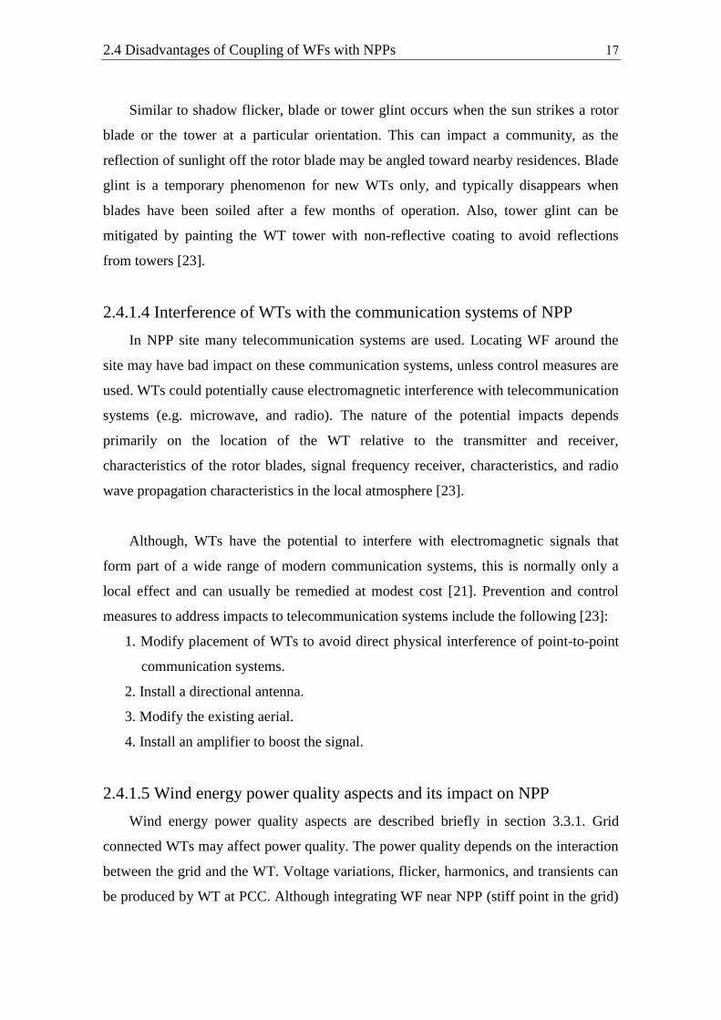
wave propagation characteristics in the local atmosphere [23].
Although, WTs have the potential to interfere with electromagnetic signals that
form part of a wide range of modern communication systems, this is normally only a
local effect and can usually be remedied at modest cost [21]. Prevention and control
measures to address impacts to telecommunication systems include the following [23]:
1. Modify placement of WTs to avoid direct physical interference of point-to-point
communication systems.
2. Install a directional antenna.
3. Modify the existing aerial.
4. Install an amplifier to boost the signal.
2.4.1.5 Wind energy power quality aspects and its impact on NPP
Wind energy power quality aspects are described briefly in section 3.3.1. Grid
connected WTs may affect power quality. The power quality depends on the interaction
between the grid and the WT. Voltage variations, flicker, harmonics, and transients can
be produced by WT at PCC. Although integrating WF near NPP (stiff point in the grid)

Chapter 2. Literature Survey 18
decreases the power quality problems of WF, this may have a side effect on the NPP
auxiliaries and therefore on the NPP operation. This disadvantage can be solved by
proper technical solutions, which will be selected according to technical studies and
simulations for case by case of each problem.
2.4.1.6 Lower energy production from WF
Energy plan in Egypt is to site WF in sites of highest wind speeds in the country so
as for highest energy generation for the installed capacity. On the other hand, idea of
coupling mainly depends on siting WF around or near NPP or large fossil-fueled power
plant, and this site in most cases has lower wind speeds compared to other sites of best
wind speeds in the country. This means lower energy production for the same installed
WF capacity.
This disadvantage can be compensated by other technical and economic benefits of
the coupling which are illustrated in this thesis. So, a detailed techno-economical study
considering different technical and economic factors of the two choices should be
conducted to get the right choice. Also, using taller blades and towers for WTs can
increase the total energy production of the WF and so overcome the problem.
2.4.2 Accident hazards from WF
WF accidents may have no major impact in site containing WF alone. In case of
coupling, part of WTs are located near NPP building and human activities in the plant.
Therefore, the occurrence of accident may lead to major consequences on the humans
and / or the operation of the NPP. So, before the construction of WF, these hazards must
be considered carefully and proper measures must be taken to minimize the possibility
of occurrence of these accidents.
The wind energy industry enjoys an outstanding health & safety record [25].
However, it involves mechanical hazards characteristic of rotating machinery, as well as
electrical hazards typical of electrical production equipment. To minimize such risks an
offset from human normal activities is adopted according to different local, national and
international norms, regulations and laws [26].

19 2.4 Disadvantages of Coupling of WFs with NPPs
2.4.2.1 Fire hazards
The risk of fire at WFs, or the risk of fire damage to WT generators, is very low.
WTs manufactured today incorporate the highest quality and safety standards, but the
potential for a fire always exists when electronics and flammable oils and hydraulic
fluids exist in the same enclosure. With normal maintenance and servicing practices in
place, a WF will not impose an increased fire hazard to the host community. Fires due
to machine failure in modern WTs are extremely rare. Cases of fire damage to land
neighbouring WFs are practically nonexistent [25].
2.4.2.2 Unique industrial risks
The blade system in a WT has incorporated in it mechanisms designed to avoid
excessive rotational speeds, including blade feathering and hydraulic and friction
braking. Blade failure could still occur ejecting the blade away for a distance from the
machine. Stress and vibration could cause tower failure. Failure mode analysis and
safety zones around WT must be used at the design and site selection stage [26].
Several potential major types of accidents can be considered for WTs:
1. Turbine tower failure, but a properly constructed WT poses negligible risk of this
type [27].
2. Blade failure and ejection, which may affect public safety, although overall risk of
blade throw is extremely low [23, 25]. There are some blade throw management
strategies illustrated in [23] & [26].
2.4.2.3 Aviation operations hazards (Aircraft safety)
Near NPP site, usually there is an airport for servicing the NPP operating staff long
transportations and required urgent maintenance jobs. There are basically two ways in
which the construction of a WT or WF may impact upon aviation operations [28]:
1. The physical obstruction caused by a tall structure:
In addition to the hazard posed to aircraft in approaching or departing from an
airfield, WTs can also pose a potential danger to aircraft flying at low level for any
other reason [26, 28]. The Obstacle Limitation Surface (OLS) is a series of

Chapter 2. Literature Survey 11
surfaces that set the height limits of objects around an airport. The height of each
WT will need to be individually reviewed to check if any part of the machine will
protrude through the OLS surface [25].
2. The effects on communications, navigation and surveillance systems:
WTs could potentially cause electromagnetic interference with aviation radar and
telecommunication systems (e.g. microwave, television, and radio) [23].
Prevention and control measures to address this impact are illustrated in [23] and
[25].

11
Chapter 3
Connecting WF and NPP to the Same Point
in the Grid
In this chapter, benefits of coupling on the grid integration issues of WFs are
presented. A case study is used to verify the benefit of coupling on voltage quality at
PCC of WF. After that, the benefit of increasing reliability and availability of NPP EPSs
by the on-site WF is discussed. A study using MARKOV process is conducted for
verification and quantification of this benefit.
3.1 Benefits of coupling on the grid integration issues of
WF
Based on a number of parameters, such as grid stiffness, transmission voltage
levels, WT topology, Transmission System Operators (TSOs) issued a number of
requirements for WTs to fulfill in order to get grid connection agreement. These
requirements were called grid codes, and they became more demanding as wind
penetration levels grew [29]. Although, the grid codes regarding wind power are
country specific, the grid codes of most countries generally aim to achieve the same
thing. Electricity networks are constructed and operated to serve a huge and diverse
customer demographic [30].
3.1.1 Voltage quality at the coupling point of WF
Grid integration of WF affects the power quality. The power quality depends on the
interaction between the grid and the WT. Figure 3.1 shows a classification of different
power quality phenomena [18]. The scope here will be on the voltage quality aspects. In
grid codes a set of requirements are imposed to cope with problems arising due to rapid
voltage changes/jumps, voltage flicker and harmonics.

Chapter 3. Connecting WF and NPP to the same point in the grid 11
Figure 3.1: Classification of different power quality phenomena
The voltage quality aspects are [18]:
1. Voltage variations: which are changes in the RMS value of the voltage during a
short period of time, mostly few minutes. If wind power is introduced, voltage
variations also emanate from the power produced by the WT.
2. Flicker: it is the traditional way of quantifying voltage fluctuations. The method is
based on measurements of variations in the voltage amplitude (i.e. the duration
and magnitude of the variations). Flicker from WTs occurs in two different modes
of operation: continuous operation (due to power fluctuations) and switching
operations.
3. Voltage harmonics: they are virtually always present in the utility grid. Nonlinear
loads, power electronic loads, and rectifiers and inverters in motor drives are some
sources that produce harmonics. Fixed-speed WTs are not expected to cause
significant harmonics and inter-harmonics. Variable-speed WTs equipped with a
converter produce harmonic currents during continuous operation.
4. Transients: they seem to occur mainly during the startup and shutdown of fixed
speed WTs. The transients may reach a value of twice the rated WT current and
may substantially affect the voltage of the low-voltage grid. The voltage transient
can disturb sensitive equipment connected to the same part of the grid.
3.1.1.1 Main requirement for WF grid integration
Short circuit capacity (SSC) is the product of the pre-fault voltage (or rated voltage)
and the current which would flow if a three-phase symmetrical fault were to occur (Eq.
3.1). SSC is a useful parameter which gives an immediate understanding of the capacity
of the circuit to deliver fault current and resist voltage variations [21, 31]. The short

13 3.1 Benefits of coupling on the grid integration issues of WF
circuit capacity in a given point in the electrical network is a measure of its strength that
has a heavy influence [19, 21, 31]. The ability of the grid to absorb disturbances is
directly related to the short circuit capacity [19].
Ssc (MVA) = √3 × line voltage (KV) × short circuit current (KA) (3.1)
Figure 3.2: Equivalent circuit [19]
Any point (P) in the network can be modeled as an equivalent circuit as shown in
Figure 3.2. Far away from the point the voltage can be taken as constant (US) i.e.
infinite bus. The short circuit capacity SSC in MVA can be found using Eq. 3.1 as US2 /
ZL where ZL is the magnitude of the line impedance. Variations in the load (or
production) in (P) causes current variations in the line and these in turn a varying
voltage drop (ΔU) over the line impedance ZL └ θL. It is obvious from Figure 3.2, that if
the impedance ZL is small then the voltage variations at (P) will be small (the grid is
strong) and consequently, if ZL is large, then the voltage variations will be large (the
grid is weak) [18, 19].
Stiff grid and weak grid are relative terms with respect to installation [19], so it is
important to compare the size of equipment to the strength of the power system. A
simple comparison is to divide the system strength by the equipment capacity, which is
named the Short Circuit Ratio (RSC) [19, 31]. A high RSC means good performance and
a low RSC means trouble [31].
(3.2)
Where:
PE: Equipment installed capacity (MW)

Chapter 3. Connecting WF and NPP to the same point in the grid 14
Another characteristic grid measure is the grid impedance angle at PCC (Ψk) [32]:
(
) (3.3)
Where:
in Figure 3.2: ZL └ θL= RL +j XL
Ψk: Grid impedance angle at PCC;
RL: Short circuit resistance of the grid
XL: Short circuit reactance of the grid
The main requirement for grid integration of WF is the limitation of voltage
deviation caused by the WTs at the PCC, for which 2% of nominal voltage is a
commonly established limit. The short circuit power level at PCC is the crucial value
for the permissible installed power ratings [33]. The grid is strong with respect to the
WF if RSC is above 20, so the variations in voltage are minor and predictable. The grid
is weak with respect to the WF if RSC is below 10 [16, 19].
3.1.1.2 Fulfillment of the main requirement for WF grid integration using
Coupling
High short circuit capacity at the PCC allows integration of large WF without
negative effect on the voltage quality. The NPP PCC with the grid has very high short
circuit level. The short-circuit level at PCC decreases, as the distance of PCC from the
substation increases [16]. So integrating WF near NPP will have a positive impact on
voltage quality instead of integrating it in remote area with low short circuit level.
The Egyptian Energy plan is to locate WFs in areas with the highest wind speeds in
the country to maximize the energy yield of the installed capacity. This leads to locating
WFs in the same area on the coast of Suez Bay, which may has lower short circuit
capacity compared to the PCC of NPP with the grid. In this thesis, it is proposed to
locate part of the future planned WFs near NPP if wind resource is promising. This
coupling will allow integration of large capacity WF without negative effect on voltage
quality due to the high short circuit capacity existed at the PCC.

15 3.1 Benefits of coupling on the grid integration issues of WF
3.1.1.3 Case study illustrating the effect of short circuit capacity on the
voltage quality aspects of WF
This study is conducted to illustrate the positive impact on voltage quality aspects
when integrating WFs near NPPs or large thermal power plants, if the wind resource is
good. PCC voltage profile of two choices will be compared, these choices are as
follows:
1. Locating WFs as it is in the Egyptian Energy plan, which is based on maximizing
energy yield of installed capacity. This means locating them on the shore of Suez
Bay where short circuit power level may be small compared to other points in the
grid;
2. Locating part of the future planned WFs, through coupling, near NPP, if wind
resource is promising in areas such as El Dabaa.
The assessment is performed according to the methods given in the IEC 61400-21
[34], which can be summarized as follows:
Steady-State voltage change:
The steady-state voltage change for one WT is given by Equation (3.4), and for the
whole WF the steady state voltage change can be estimated by Equation (3.5). S60 and Ø
can be calculated from P60 and Q60 [19, 34].
60
{ ( )} Only valid for cos(Ψk+Ø) > 0.1 (3.4)
60
{ ( )} Only valid for cos(Ψk+Ø) > 0.1 (3.5)
Where:
dss: Steady state voltage change of the grid at PCC due to one WT (normalised to
nominal voltage);
dss∑: Steady state voltage change of the grid at PCC due to the WF (normalised to
nominal voltage);
S60: Apparent power at the 1-min. active power peak;
Ssc: Short circuit power level of the grid at PCC;

Chapter 3. Connecting WF and NPP to the same point in the grid 16
Ψk: Grid impedance angle at PCC;
Ø: Phase angle between voltage and current; and
NWT: Number of WTs in the WF.
Flicker distortion:
The flicker distortion for continuous operation of one WT can be calculated from
Equation (3.6), and for the whole WF the flicker emission can be estimated by Equation
(3.7) [19, 34].
( )
(3.6)
√ ( )
(3.7)
Where:
Plt: Flicker distortion (emission) of one WT;
Plt∑: Flicker distortion (emission) of the whole WF;
c(Ψk, Va): Flicker coefficient;
Va: Annual average wind speed at hub height; and
Sn: Apparent power of the WT at rated power.
Switching operations:
For switching operations two criterions must be checked: the voltage change due to
the inrush current of a switching and the flicker effect of the switching. The control
system of a WF ensures that two or more WTs in a WF are not switched on
simultaneously. Therefore, only one WT has to be taken into account for the calculation
of the voltage change. The worst case of switchings concerning the voltage change is
the cut-in of the WT at rated wind speed, and can be calculated using Equation (3.8)
[19, 34].
( )
(3.8)

17 3.1 Benefits of coupling on the grid integration issues of WF
Where:
dso: Switching operations voltage change of the grid at PCC (normalised to nominal
voltage); and
ku(Ψk): Voltage change factor.
On the other hand, the flicker effect has to be calculated for both types of
switching: for the cut-in at cut-in wind speed and for the cut-in at rated wind speed. The
flicker emission due to switching operations of a single WT can be estimated from
Equation (3.9), and Equation (3.10) can be used for the whole WF. The flicker effect
has to be calculated for both types of switching: for the cut-in at cut-in wind speed and
for the cut-in at rated wind speed [19, 34].
( ) ( )
(3.9)
( ) ( )
(3.10)
Where:
Plt: Flicker distortion (emission) of one WT;
Plt∑: Flicker distortion (emission) of the whole WF;
kf(Ψk): Flicker step factor; and
N120: Number of switchings within a 120-minute period.
Definitions for different factors and coefficients mentioned above can be found in
details in [34]. Also, methods to calculate their values and some examples are provided
in [34].
Two types of WTs are selected, Type A and Type D. Description of different WT’s
Types and the configuration of each type can be found in [18]. WTs are selected as
typical representatives of solutions and developmental directions in wind technology.
Table 3.1 shows the data for the selected sites. Tables 3.2 and 3.3 show the data for the
used WTs. Four scenarios will be compared, with the details illustrated in Table 3.4.
Appling Equations (3.4) to (3.10), to all scenarios, results given in Table 3.5 can be
obtained. Short circuit power level of the grid at PCC has a significant effect on the

Chapter 3. Connecting WF and NPP to the same point in the grid 18
calculated parameters for both types of WTs used (Type A and D). As, the short circuit
power level of the grid at PCC increases, all these parameters decrease, and so better
voltage quality at PCC.
Table 3.1: Data of the proposed sites
El Dabaa Zafarana
Annual average wind speed (m/s) 7.5 8.5
Nominal voltage of the grid (KV) 500 220
Short circuit power level of the grid (MW), Ssc 1000 600
Grid impendance angle (°), (Ψk) 85° 50°
Table 3.2: Data of the used Type A WT [19]
Wind Turbine Type Type A
Hub height (m) 50
Rated power (KW), Pn 600
Rated apparent power (KVA), Sn 607
Rated voltage (V), Un 690
Rated current (A), In 508
Max. power (KW), P60 645
Max. Reactive power (KVAR), Q60 114
Flicker:
Grid impedence angle Ψk (°): 30° 50° 70° 85°
Annual average wind speed Va (m/s): Flicker coefficient, c(Ψk, Va):
6.0 7.1 5.9 5.1 6.4
7.5 7.4 6.0 5.2 6.6
8.5 7.8 6.5 5.6 7.2
10.0 7.9 6.6 5.7 7.3
Switching operations:
Case of switching
operation:
Cut-in at cut in wind speed Cut-in at rated wind speed
Max number of
switchings N10 3 1
Max number of
switchings N120 30 8
Grid impedence
angle Ψk (°) 30° 50° 70° 85° 30° 50° 70° 85°
Flicker step factor
kf(Ψk) 0.35 0.34 0.38 0.43 0.35 0.34 0.38 0.43
Voltage change
factor ku(Ψk) 0.7 0.7 0.8 0.9 1.30 0.85 1.05 1.60

19 3.1 Benefits of coupling on the grid integration issues of WF
Table 3.3: Data of the used Type D WT [35]
Wind Turbine Type Type D
Hub height (m) 85
Rated power (KW), Pn 2000
Rated apparent power (KVA), Sn 2000
Rated voltage (V), Un 690
Rated current (A), In 1660
Max. power (KW), P60 2011
Max. Reactive power (KVAR), Q60 14.3
Flicker:
Grid impedence angle Ψk (°): 30° 50° 70° 85°
Annual average wind speed Va (m/s): Flicker coefficient, c(Ψk, Va):
3.0 3 3 2 2
6.0 3 3 2 2
9.0 3 3 2 2
12.0 3 3 2 2
15.0 3 3 2 2
Switching operations:
Case of switching
operation:
Cut-in at cut in wind speed Cut-in at rated wind speed
Max number of
switchings N10 10 1
Max number of
switchings N120 120 12
Grid impedence
angle Ψk (°) 30° 50° 70° 85° 30° 50° 70° 85°
Flicker step factor
kf(Ψk) 0.1 0.1 0.1 0.1 0.1 0.1 0.1 0.1
Voltage change
factor ku(Ψk) 0.2 0.1 0.1 0.0 0.9 0.7 0.3 0.1
Table 3.4: Scenarios under study
Site El Dabaa Zafarana
WT Type Type A Type D Type A Type D
Installed Capacity 333*0.6 MW
= 199.8 MW
100*2 MW
= 200 MW
333*0.6 MW
= 199.8 MW
100*2 MW
= 200 MW
Scenario Scenario 1 Scenario 3 Scenario 2 Scenario 4

Chapter 3. Connecting WF and NPP to the same point in the grid 31
Table 3.5: Calculation results for voltage quality aspects for all scenarios
Site El Dabaa Zafarana El Dabaa Zafarana
WT Type Type A Type A Type D Type D
Scenario Scenario 1 Scenario 2 Scenario 3 Scenario 4
Va (m/s) 7.5 8.5 7.5 8.5
S60 (MVA) 0.655 0.655 2.01105 2.01105
Sn,i (MVA) 0.607 0.607 2 2
SSC (MVA) 1000 600 1000 600
Ø (°) 10 10 0.41 0.41
Ψk (°) 70 50 70 50
Number of WTs 333 333 100 100
Steady-state voltage change (dss)
dss (%) (One WT) 0.00011 0.00055 0.00067 0.00214
dss∑ (%) (100 WT) 0.03788 0.18176 0.06743 0.21360
Flicker distortion (Plt) (%)
C(Ψk, Va) 5.2 6.5 2 3
Plt (%) 0.003 0.007 0.004 0.010
Plt∑ (%) 0.058 0.120 0.040 0.100
Switching Operations:
Voltage change due to cut-in at rated wind speed (dso)
ku(Ψk) 1.05 0.85 0.3 0.7
dSO (%) 0.00063735 0.0008599 0.0006 0.00233333
Flicker distortion due to cut-in at cut-in wind speed (Plt ) (%)
N120 30 30 120 120
kf(Ψk) 0.38 0.34 0.1 0.1
Plt (%) 0.005 0.008 0.007 0.012
Plt∑ (%) 1.764 2.630 0.706 1.176
Flicker distortion due to cut-in at rated wind speed (Plt ) (%)
N120 8 8 12 12
kf(Ψk) 0.38 0.34 0.1 0.1
Plt (%) 0.004 0.005 0.003 0.006
Plt∑ (%) 1.171 1.746 0.346 0.576

31 3.1 Benefits of coupling on the grid integration issues of WF
3.1.2 Active power / frequency control capability
To provide frequency control, the WTs must operate below the potential output
level for the current wind conditions. For All types of WTs, load-frequency control can
be obtained by slightly increasing the nominal blade pitch angle, deloading the WT by a
corresponding amount. Thus, the WT output can be adjusted in sympathy with
frequency variations, akin to governor control on a conventional generator. Such an
approach is feasible with conventional pitch control. For variable-speed WTs, power
output regulation can also be achieved by varying the rotor speed – a small decrease in
rotational speed away from the optimum tip-speed ratio will cause a reduction in
electrical output [22]. So, the WT pitch angle could be adjusted for partial output, while
maintaining a reserve margin of, say, 1–3 % of rated output (delta control). There are
other control strategies that can be implemented which are illustrated in [22].
3.1.2.1 Benefits of coupling on the active power / frequency control
capability of the WF
A grid employing large amounts of wind energy requires the balance of the system
to be highly flexible to respond to the increased variability of the net load. Therefore,
when wind energy penetration in the power system becomes high, the use of storage
units becomes interesting. At the same time, storage units may ensure power delivery
from the WF, even when the wind speed is low. Consequently, storage units can provide
large WFs with power regulation capabilities, which can enable WFs to replace, and not
just to supplement, other power plants. Besides a capacity reduction of other power
plants, such regulation capabilities may further reduce the requirement for spinning
reserve and thus reduce the total fuel costs in the power system [32].
On the other hand, NPPs generally provide constant, base load power and are most
economic when operated at constant power levels. Operating NPPs in load-following
modes decreases the plants' annual energy output and increases the levelized cost of
energy. By coupling energy storage facility to NPPs, the reactor remains at nearly
constant output, while cycling the energy storage facility in response to the variability of
the net load. Meanwhile, the added energy storage facility can work as onsite power
source to supply safety related loads during Loss of Off-site Power (LOOP) and Station

Chapter 3. Connecting WF and NPP to the same point in the grid 31
Black Out (SBO) accidents, which increases the capacity and availability of the onsite
power supply. Finally, the energy storage facility can store the energy spilled through
the NPP turbine by-bass valves.
Therefore, the addition of energy storage facility to the system will have technical
and economical benefits for both WF and NPP. Different energy storage technologies
are illustrated in [33]. Some research works were done in the coupling of hydrogen
storage facility to wind-NPP system, as in [4, 36, 37]. Hydrogen can be generated from
part of the generated heat in the reactor core of NPP and from electrolyzers which are
supplied from WF. Also, NPP already has in its electrical system a large sets of Lead-
Acid battery banks. These banks can be integrated to the energy storage facility.
3.1.3 Reactive power / voltage control capability
WFs that are large enough to be connected to the transmission system tend to be
erected in remote areas or offshore because of their dimension and impact on the
scenery. Given that the node voltage is a local quantity, it can be difficult to control the
voltage at these distant places by use of conventional power stations elsewhere in the
grid. Therefore, WTs have to have reactive power / voltage control capabilities. The
reactive power / voltage control capabilities of WTs erected in large-scale WFs and
connected to the transmission network become increasingly important [18]. The
exchange rate and level of reactive power with the grid is specified by the TSO [29].
Utilities around the world have started requiring WFs to maintain a power factor of 0.95
or higher [16]. WF reactive power requirements stated by US Federal Energy
Regulatory Commission are illustrated in [16]. Danish grid code requirements for WF
reactive power are given in [29]. TSO in Germany gives requirements that must be
fulfilled by any power plant to be connected to grid regardless of its type. These
requirements are presented in Figure 3.3. This figure shows one of the three possible
variants of TSO demands. TSO selects one of the versions on the basis of relevant
network characteristics [30].

33 3.1 Benefits of coupling on the grid integration issues of WF
Figure 3.3: Reactive power control requirement as a function of grid voltage (EON
Netz GmbH) [30]
3.1.3.1 Benefits of coupling on reactive power / voltage control capability
of WF
There are many solutions for supplying reactive power within WF. Some of them
are: increasing converter size for Types C and D WTs [18], provision of centralized
versus distributed reactive compensating mechanically switched technologies, and
rotating synchronous compensators. Vestas turbines have estimated that WTs with a
reactive power capability corresponding to a power factor of 0.9 at rated active power
output incur the costs shown in Table 3.6 over WTs constructed for unity power factor
[22].
Table 3.6: Cost implications of WT power factor capability of 0.9 [22]
Cost increase (%) Method
100 SVC at MV
41-53 Converter resizing
47 Passive elements at LV
By coupling of WF with the adjacent NPP, the NPP can carry the task of reactive
power/ voltage support perfectly. This is due to the large capacity synchronous
generator used in NPPs which has a capability to supply large amounts of reactive
power in cheap costs and with high reliability and availability. For WF utilizing Type A

Chapter 3. Connecting WF and NPP to the same point in the grid 34
or B WTs, NPP will supply reactive power for the WF collecting system, WTs
themselves, and voltage support to PCC. This will achieve the grid requirements of
reactive power / voltage control by WF. Also, avoiding the use of switched capacitors at
each WT and so transients associated with them. For WF utilizing Type C or D WTs,
each WT will work at unity power factor at the low voltage side of its step up
transformer, which connects it to the collecting system. NPP will supply reactive power
for the WF collecting system, and carry the task of voltage support at PCC. Therefore,
grid requirements of reactive power / voltage control by WF is achieved without
increasing the converters rating, and so lower cost.
3.2 Increasing Reliability and Availability of NPP EPSs
by the on-site WF
The safe and economic operation of a NPP requires the plant to be connected to an
electrical grid system that has adequate capacity for exporting the power from the NPP,
and for providing a reliable electrical supply to the NPP for safe startup, operation and
normal or emergency shutdown of the plant. An important characteristic of all NPPs is
that after a nuclear reactor is shut down, it continues to produce a significant amount of
heat for an extended period. Hence the reactor cooling systems must continue to operate
for several days after a reactor shuts down, to prevent overheating and damage to the
reactor core. Therefore, reliable cooling arrangements must be provided, and this
requires robust and diverse sources of reliable electrical supply [38]. This reliable
electrical supply comes either from the grid (off-site power), or from on-site emergency
back-up power, such as batteries, diesel generators or gas turbines [39].
The transmission system is the source of power to the offsite power system, and it
has higher availability and reliability than the on-site emergency power system because
of the diverse and multiple generators connected to the transmission system. Hence
NPPs generally consider offsite power as the primary source (preferred source) of
power for cooling down the reactor during normal and emergency shutdowns [38]. The
reliability of off-site power is usually assured by two or more physically independent
transmission circuits to the NPP to minimize the likelihood of their simultaneous

35 3.2 Increasing Reliability and Availability of NPP EPSs by the on-site WF
failure. Similarly, the reliability of on-site power is enhanced by sufficient
independence, redundancy and testability of batteries, diesel generators, gas turbines
and the on-site electric distribution systems to perform safety and other functions even
if a single failure occurs [39].
The full electrical load of the auxiliaries of a NPP is typically 5–8% of the NPP
rated load. Hence the electrical connection to the NPP must be able to supply this load
during reactor startup, and immediately after reactor shutdown, whether from a planned
shut down or an unplanned reactor trip that may occur at any time [38].
3.2.1 NPP electrical system
The typical structure of NPP electrical systems is illustrated in Figure 3.4. The
onsite power system is the name of the electrical components and switchgears in the
system, which is supporting the process system components with electric power. All the
station auxiliaries are divided into two main groups. First is the non class 1E loads, and
they should have two independent power sources with automatic switchover provisions.
They allow power interruption during automatic switchover and may not require power
after reactor scram. The second is the EPSs, with a simplified single line diagram shown
in Figure 3.5. The purpose of the EPSs is to provide the plant with the necessary power
in all relevant conditions within the design basis so that the plant can be maintained in a
safe state after postulated initiating events, in particular during the LOOP accident [38].
The EPSs can be powered from the normal power supply or (optionally) from the
alternative on-site power supplies as shown in Figure 3.5 [40].

Chapter 3. Connecting WF and NPP to the same point in the grid 36
Figure 3.4: Simplified single line diagram of the NPP electrical system [40]
EPSs are generally divided into three systems as follows [40]:
1. An AC power system: the assigned AC loads allow a certain interruption of the
power supply.
2. A DC power system: that supplies DC loads without interruption from a battery.
This DC system includes a battery charger that is connected to the AC system of
the EPSs.
3. A non-interruptible AC power system: that is supplied by the DC power system of
the EPSs by means of inverters and is also connectable to the AC power system of
the EPSs. The most important components of the safety systems belong to this
group.

37 3.2 Increasing Reliability and Availability of NPP EPSs by the on-site WF
Figure 3.5: A simplified single line diagram of EPSs block [40]
3.2.2 The benefit of adjacency of WF & NPP on the NPP
electrical system
To decrease the probability of SBO accident, some NPPs chose to add additional
emergency ac power sources, typically diesel generators or gas turbine generators [40].
In case of coupling, there is new onsite power source which is the WF. By integrating
WF in the NPP electrical system using proper measures, the reliability of onsite power
is enhanced by sufficient independency and redundancy of batteries, diesel generators,
gas turbines and the new power source (WF).
This integration of onsite WF in the EPSs has some benefits:
1. Increasing the reliability and availability of power source in the EPSs by adding
another type of generation (WF). Formerly, tens and hundreds of WTs have been
distributed over an area, offer the advantages of wind diversity and distributed
reliability [22].

Chapter 3. Connecting WF and NPP to the same point in the grid 38
2. Increasing the time of availability of power source in the EPSs in case of LOOP
accident. This is due to the lower fuel consumption of diesel generators.
3. Allowance to supply more loads than safety related loads due to the increase on the
onsite power source capacity.
However, this integration requires proper technical measures to work probably. The
integration of WF in the NPP electrical system can be achieved by providing a reliable
connection from WF output to the bus bar of alternative onsite power supply in the NPP
electrical system (Figure 3.5). In case of LOOP accident, WF or part of it will be
allowed to work in parallel to the standby diesel generators as wind-diesel system. In
wind-diesel system, as the wind power or load changes, the diesel power must change
since the diesel is required to balance the difference between the required load and the
wind generation. In case of diesel generators fails due to any reason, energy storage
facility may be used to smooth out fluctuations in the load and wind power [18]. In this
case, the WF has to be connected to the battery bus in the EPSs (Figure 3.5). This is
achieved by the use of rectifiers for the WF output or the power electronic devices
impeded in WTs themselves. The power generated from the WF will charge the
batteries and supplies power to both DC loads and uninterruptable AC loads. Supplying
power to AC loads which allow certain interruption of power will require an inverter.
Therefore, all EPSs loads can be supplied even if diesel generators fail to supply power.
3.2.3 Using MARKOV Process to illustrate EPS’s Reliability and
Availability enhancement using on-site WF
Availability is defined as the probability that the system is operating properly when
it is requested for use. In other words, availability is the probability that a system is not
failed or undergoing a repair action when it needs to be used. On the other hand,
reliability represents the probability of the system to perform its required functions for a
desired period of time without failure in specified environments with a desired
confidence.
As stated above, the reliability and availability of EPS can be enhanced using
available on-site WF. A case study is conducted using a NPP in El Dabaa site and a WF

39 3.2 Increasing Reliability and Availability of NPP EPSs by the on-site WF
is erected near it. For calculations simplicity, only two WTs from the WF will be
integrated to the EPS.
The reliability models of Ordinary Generation Units (OGUs) are originated from
reliability data of failures and repair rates and the two state models covers all aspects of
OGUs [42]. Figure 3.6 represents the Markov graph for single OGU. An OGU has a
failure rate λ and a repair rate µ based on the reliability data which have been collected
through the field. When a generation unit fails, the state of the system will change by
the rate of λ from operating mode to failure mode. Similarly, when a generation unit is
going to be repaired, the state of the system will change by the rate of µ from failure to
operating mode. In this two state model OGUs are assumed to produce 0 MWs in the
failure mode and to produce the rated power in the operating mode [42].
When a WT is going to be modeled for reliability studies, the two state model will
not work properly. This is due to the behavior of WT compared with OGU. WT has a
variable nonlinear output curve in different wind speeds shown typically in Figure 3.7.
Several methods have been proposed to cover this difference, which mainly fall into two
categories: the analytical and simulation methods. Simulation circumstances like Monte
Carlo and the Auto Regressive and Moving Average are used to model the WFs for
reliability assessment purposes. These methods need long term data of wind speed
which these kinds of data may not be available for certain wind sites. The analytical
methods are also used to model the WTs for many years. Using analytical methods
reduce the computational efforts in comparison with the simulation methods. The multi-
state model of output power has been used for reliability analysis of WF. The
probability of occurrence for discrete output power states are considered by use of
Probability Distribution Function (PDF) of wind speed data. The severity of the
variation in the wind speed pattern will not be detected if the PDF based method is used
for modeling the wind speed [42].
The Markov graph for single WT is shown in Figure 3.8. The arrows indicated by
Øs represent the probability of transition between output power states in a single WT
which happen due to variation of wind speed [42].
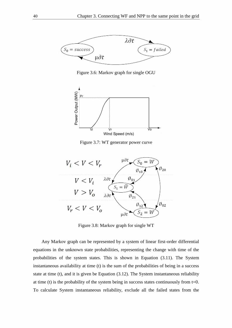
Chapter 3. Connecting WF and NPP to the same point in the grid 41
Figure 3.6: Markov graph for single OGU
Figure 3.7: WT generator power curve
Figure 3.8: Markov graph for single WT
Any Markov graph can be represented by a system of linear first-order differential
equations in the unknown state probabilities, representing the change with time of the
probabilities of the system states. This is shown in Equation (3.11). The System
instantaneous availability at time (t) is the sum of the probabilities of being in a success
state at time (t), and it is given be Equation (3.12). The System instantaneous reliability
at time (t) is the probability of the system being in success states continuously from t=0.
To calculate System instantaneous reliability, exclude all the failed states from the

41 3.2 Increasing Reliability and Availability of NPP EPSs by the on-site WF
transition matrix A. The new matrix A’ contains the transition rates for transitions only
among the success states (the ‘reduced’ system is virtually functioning continuously
with no interruptions). The reduced system is represented by Equation (3.13). After that,
the System instantaneous Reliability can be calculated using Equation (3.14).
[ ( )
( )
( )
]
[
] [
( )
( ) ( )
] Or
( ) (3.11)
Where:
Pi(t): Probability of system to be in state (i) function in time;
A: Transition rate matrix;
N: Number of states; and
α10: Transition rate from state (1) to state (0).
( ) ( ) (3.12)
Where:
S: set of success states of the system
F: set of failure states of the system
( ) (3.13)
( ) (3.14)
The Markov approach will be applied under the following basic assumptions:
1. Constant failure and repair rates are considered;
2. Only single repairman is permitted; and
3. Perfectly reliable switching is assumed.
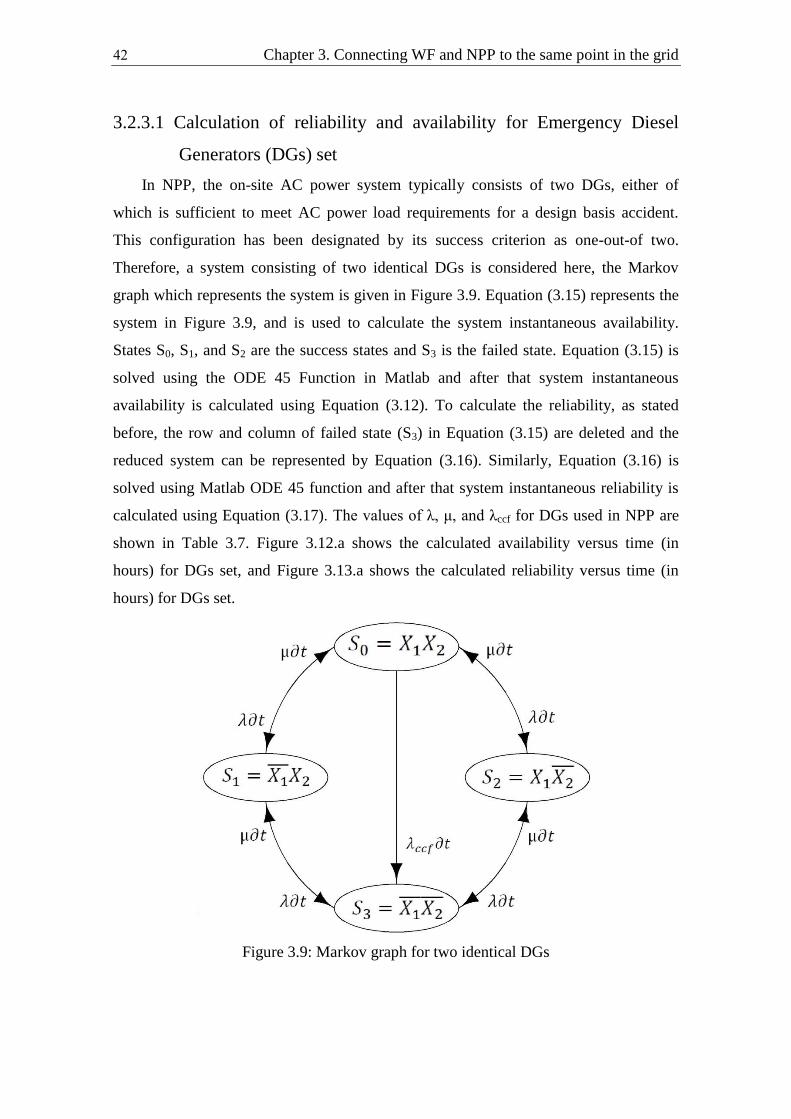
Chapter 3. Connecting WF and NPP to the same point in the grid 41
3.2.3.1 Calculation of reliability and availability for Emergency Diesel
Generators (DGs) set
In NPP, the on-site AC power system typically consists of two DGs, either of
which is sufficient to meet AC power load requirements for a design basis accident.
This configuration has been designated by its success criterion as one-out-of two.
Therefore, a system consisting of two identical DGs is considered here, the Markov
graph which represents the system is given in Figure 3.9. Equation (3.15) represents the
system in Figure 3.9, and is used to calculate the system instantaneous availability.
States S0, S1, and S2 are the success states and S3 is the failed state. Equation (3.15) is
solved using the ODE 45 Function in Matlab and after that system instantaneous
availability is calculated using Equation (3.12). To calculate the reliability, as stated
before, the row and column of failed state (S3) in Equation (3.15) are deleted and the
reduced system can be represented by Equation (3.16). Similarly, Equation (3.16) is
solved using Matlab ODE 45 function and after that system instantaneous reliability is
calculated using Equation (3.17). The values of λ, μ, and λccf for DGs used in NPP are
shown in Table 3.7. Figure 3.12.a shows the calculated availability versus time (in
hours) for DGs set, and Figure 3.13.a shows the calculated reliability versus time (in
hours) for DGs set.
Figure 3.9: Markov graph for two identical DGs

43 3.2 Increasing Reliability and Availability of NPP EPSs by the on-site WF
[ ( )
( )
( )
( )
]
[ ( )
( ) ( ) ]
[ ( )
( )
( )
( )]
(3.15)
Where:
P0(t): Probability function in time of state S0;
λ: Failure rate of one unit of DG;
μ: Repair rate of one unit of DG; and
λccf: Common cause failure rate of DGs set.
[ ( )
( )
( )
]
[
( )
( )
( )
] [
( )
( )
( )] (3.16)
Table 3.7: Reliability and Availability data for DGs used in NPP [43]
Symbol Value
λ 5.2*10-3
/h
μ 0.05 /h
λccf 2.59*10-4
/h
3.2.3.2 Calculation of reliability and availability for WTs set
The Markov graph which represents the system is given in Figure 3.10. The
transition between states depend on WTs condition (operate or fail) and the wind speed.
Transition between states based on WTs condition change is done through failure and
repair rates. Transition between states based on change in wind speed region is done
through Øij, which is the probability of being in wind speed region of state (i) and the
wind speed changes to be in the wind speed region of state (j). Øs are calculated based
on PDF of wind speeds in the area using Weibull distribution. Equations from (3.17) to
(3.24) represent probability density function of the 2-parameter Weibull distribution of
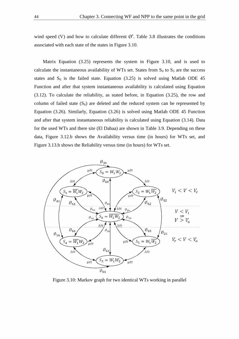
Chapter 3. Connecting WF and NPP to the same point in the grid 44
wind speed (V) and how to calculate different Øs. Table 3.8 illustrates the conditions
associated with each state of the states in Figure 3.10.
Matrix Equation (3.25) represents the system in Figure 3.10, and is used to
calculate the instantaneous availability of WTs set. States from S0 to S5 are the success
states and S6 is the failed state. Equation (3.25) is solved using Matlab ODE 45
Function and after that system instantaneous availability is calculated using Equation
(3.12). To calculate the reliability, as stated before, in Equation (3.25), the row and
column of failed state (S6) are deleted and the reduced system can be represented by
Equation (3.26). Similarly, Equation (3.26) is solved using Matlab ODE 45 Function
and after that system instantaneous reliability is calculated using Equation (3.14). Data
for the used WTs and there site (El Dabaa) are shown in Table 3.9. Depending on these
data, Figure 3.12.b shows the Availability versus time (in hours) for WTs set, and
Figure 3.13.b shows the Reliability versus time (in hours) for WTs set.
Figure 3.10: Markov graph for two identical WTs working in parallel
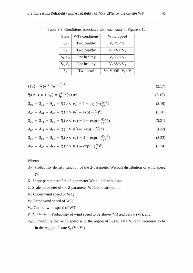
45 3.2 Increasing Reliability and Availability of NPP EPSs by the on-site WF
Table 3.8: Conditions associated with each state in Figure 3.10
State WTs conditions Wind Speed
S0 Two healthy Vi <V< Vr
S3 Two healthy Vr <V< Vo
S1, S2 One healthy Vi <V< Vr
S4, S5 One healthy Vr <V< Vo
S6 Two dead V< Vi OR Vr <V
( )
(
) ( (
))
(3.17)
( ) ∫ ( )
(3.18)
( ) ( (
) ) (3.19)
( ) ( (
) ) (3.20)
( ) ( (
) ) (3.21)
( ) ( (
) ) (3.22)
( ) ( (
) ) (3.23)
( ) ( (
) ) (3.24)
Where:
f(v):Probability density function of the 2-parameter Weibull distribution of wind speed
(v);
K: Shape parameter of the 2-parameter Weibull distribution;
C: Scale parameter of the 2-parameter Weibull distribution;
Vi: Cut-in wind speed of WT;
Vr: Rated wind speed of WT;
Vo: Cut-out wind speed of WT;
Pr (Vi<V<Vr ): Probability of wind speed to be above (Vi) and below (Vr); and
Ø06: Probability that wind speed is in the region of S0 (Vi <V< Vr) and decreases to be
in the region of state S6 (V< Vi).
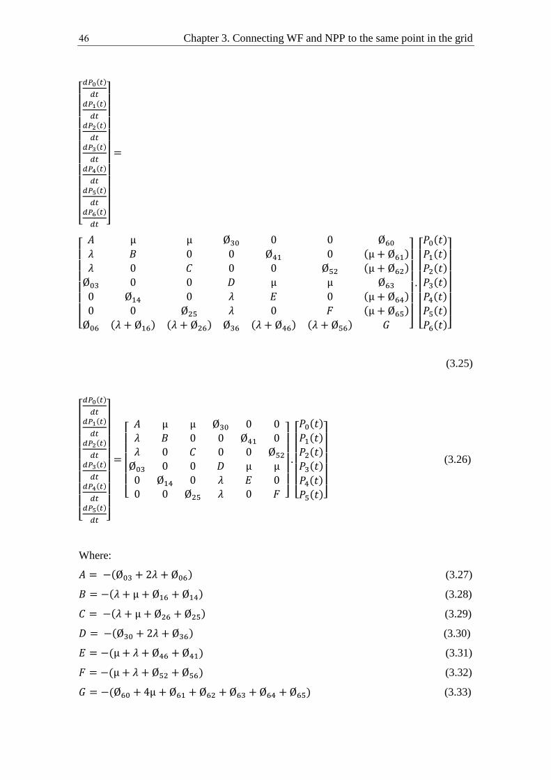
Chapter 3. Connecting WF and NPP to the same point in the grid 46
[ ( )
( )
( )
( )
( )
( )
( )
]
[ ( )
( )
( )
( )
( ) ( ) ( ) ( ) ]
[ ( )
( )
( )
( )
( )
( )
( )]
(3.25)
[ ( )
( )
( )
( )
( )
( )
]
[
]
[ ( )
( )
( )
( )
( )
( )]
(3.26)
Where:
( ) (3.27)
( ) (3.28)
( ) (3.29)
( ) (3.30)
( ) (3.31)
( ) (3.32)
( ) (3.33)
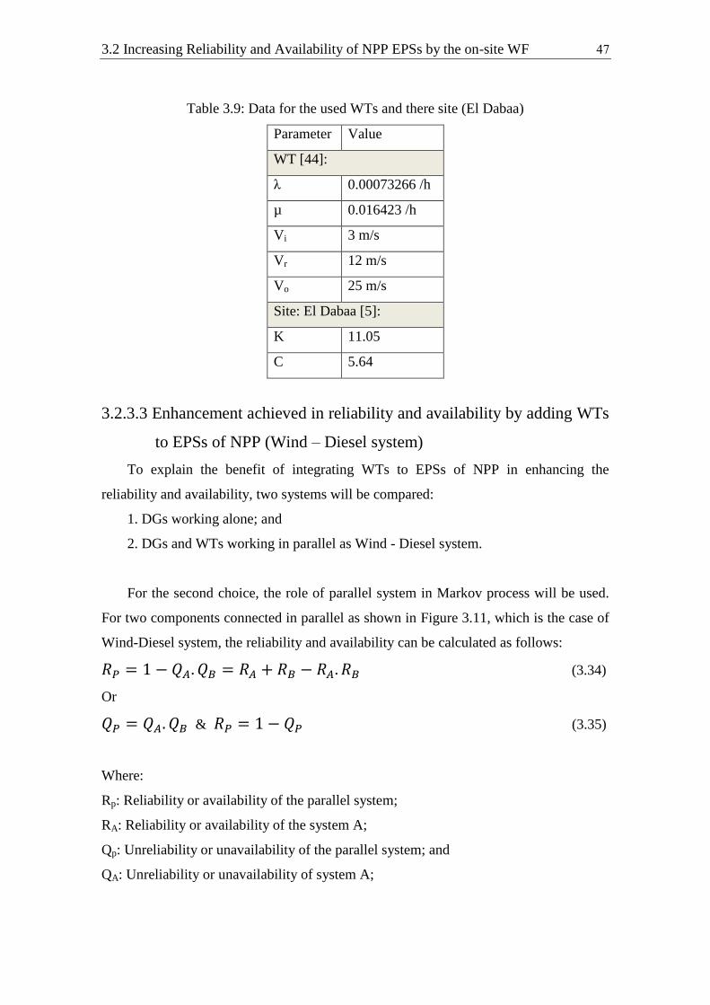
47 3.2 Increasing Reliability and Availability of NPP EPSs by the on-site WF
Table 3.9: Data for the used WTs and there site (El Dabaa)
Parameter Value
WT [44]:
λ 0.00073266 /h
µ 0.016423 /h
Vi 3 m/s
Vr 12 m/s
Vo 25 m/s
Site: El Dabaa [5]:
K 11.05
C 5.64
3.2.3.3 Enhancement achieved in reliability and availability by adding WTs
to EPSs of NPP (Wind – Diesel system)
To explain the benefit of integrating WTs to EPSs of NPP in enhancing the
reliability and availability, two systems will be compared:
1. DGs working alone; and
2. DGs and WTs working in parallel as Wind - Diesel system.
For the second choice, the role of parallel system in Markov process will be used.
For two components connected in parallel as shown in Figure 3.11, which is the case of
Wind-Diesel system, the reliability and availability can be calculated as follows:
(3.34)
Or
& (3.35)
Where:
Rp: Reliability or availability of the parallel system;
RA: Reliability or availability of the system A;
Qp: Unreliability or unavailability of the parallel system; and
QA: Unreliability or unavailability of system A;

Chapter 3. Connecting WF and NPP to the same point in the grid 48
Figure 3.11: Two systems A and B connected in parallel
Applying equations (3.34) or (3.35) using Figures 3.12.a, 3.12.b, 3.13.a & 3.13.b,
the availability and reliability of the Wind-Diesel system can be calculated. Figures
3.12.c & 3.13.c represent the availability and reliability of Wind-Diesel system
respectively. Also, they compare this case with the case of DGs working alone. These
figures illustrate the availability and reliability of each system regardless of its power
generation level. DGs sets can generate at nearly 100% of installed capacity when they
are on. However, generation from WTs (or WF) is fluctuating between 0% and 100% of
installed capacity according to the weather and WTs conditions. Therefore, to be more
accurate, minimum acceptable limit for WF generated power should be set and used in
these calculations. Under this minimum limit, the WF will be considered unavailable
and unreliable. This minimum limit depends on: NPP capacity, NPP house load during
emergencies, WF capacity, etc.
As a case study, it is assumed that 1000 MW NPP is existed and 100 MW WF is
adjacent to it. During emergency conditions, NPP requires about 2% of its installed
capacity for supplying emergency house loads, and so this counts for 20 MW.
Therefore, for WF to be reliable and available, they should supply these 20 MW which
equals 20% of its installed capacity. So, the minimum limit is 20% (or 20 MW).
Systems illustrated in Figure 3.9 and Figure 3.10 can be used in this case study. No
changes for DGs system (Figure 3.9). In Figure 3.10, instead of having two WTs
working in parallel, two parallel trains of WTs will be assumed. Each train consists of
50 MW, and should produce 20 MW as minimum limit to be available and reliable.
From WT generator power curve (Figure 3.7), and data illustrated in Table 3.9, wind
speed should be above 8.7 m/s at hub height for WF to be available and reliable.
Applying the same procedure for systems given in Figures 3.11 and 3.12 with these

49 3.2 Increasing Reliability and Availability of NPP EPSs by the on-site WF
simple changes results in Figure 3.14 and Figure 3.15 can be calculated. Figure 3.14
represents the enhancement in availability achieved by WF integration in the EPS
system, and Figure 3.15 represents the enhancement in reliability. The system’s
reliability is only enhanced in the first six hours, which are vital during emergency
conditions.
From Figures 3.12.c, 3.13.c, 3.14, and 3.15, it is clear that integrating WTs in the
EPSs of NPP enhanced the system’s availability and reliability considerably. This
enhancement is very important especially during the first hours of operation. This
integration of onsite WF to the NPP’s EPSs benefits can be summarized as follows:
1. Increasing the Reliability and Availability of power source in the EPSs by adding
another type of generation (WF). Generally, tens and hundreds of WTs have been
distributed over an area, offer the advantages of wind diversity and distributed
reliability [22].
2. Lower fuel consumption of DGs, so during LOOP accident, the availability time of
power source in the EPS will be increased.
3. Increasing the onsite power source capacity allows supplying more loads than only
safety related loads.

Chapter 3. Connecting WF and NPP to the same point in the grid 51
Figure 3.12.a: DGs set
Figure 3.12.b: WTs set
Figure 3.12.c: Wind-Diesel System versus DGs set
Figure 3.12: Availability versus time (hours)

51 3.2 Increasing Reliability and Availability of NPP EPSs by the on-site WF
Figure 3.13.a: DGs set
Figure 3.13.b: WTs set
Figure 3.13.c: Wind-Diesel System versus DGs set
Figure 3.13: Reliability versus time (hours)

Chapter 3. Connecting WF and NPP to the same point in the grid 51
Figure 3.14: Availability versus time (hours) for Wind-Diesel System and DGs set, with
minimum production of 20 MW from WF
Figure 3.15: Reliability versus time (hours) for Wind-Diesel System and DGs set, with
minimum production of 20 MW from WF
Zoom

53
Chapter 4
Aspects Related to Adjacency Between WF
and NPP
In this chapter the benefit of WFs geographical distribution is illustrated. A Case
study is conducted to evaluate the WFs geographical distribution in Egypt and its
impact on the capacity credit of wind energy in the grid.
4.1 Geographical distribution of WFs in the grid
The wind speed varies continuously as a function of time and height. Therefore,
wind energy is characterized by large variations in production. Figure 4.1 illustrates an
example of large-scale wind power production versus time in Denmark during January
2000 [18]. Just as consumer demands are smoothed by aggregation, so is the output
from WF, and geographic dispersion dramatically reduces the wind fluctuations and
there will be fewer instances of near zero or peak output [18, 22].
Figure 4.1: An example of large-scale wind power production in Denmark, January
2000 [18]
As wind energy is aggregated from multiple WTs in a WF, the short-term
variations in wind resources is attenuated as a percentage of the overall power output
[18, 16, 22]. When wind energy from multiple WFs is aggregated, minute to- hour
variation in energy is attenuated and an hour-to-day variation in wind energy production

Chapter 4. Aspects related to adjacency between WF and NPP 54
and delivery to the grid is observed. Grid system operators manage such variations
using spinning reserves [16]. With wind penetration of up to 20% of system total peak
demand, additional spinning reserves will be required. It has been found that this results
in additional cost of up to 10% of the wholesale value of wind energy [45]. So the
smoothing effect of aggregation of wind power in the grid means that the operational
penalties associated with running networks with wind may be lower than early
estimates. Thus, the extra cost of running more thermal plant as spinning reserve is
lowered [22]. A wide geographical distribution of WFs reduces the impact of the slower
variations as changing weather patterns do not affect all WTs at the same time [18].
Figure 4.2 shows the principal of aggregated wind power production based on
simulations by Pedro Rosas, where the time scale on graphics is seconds [18].
Figure 4.2: Impact of geographical distribution and additional WTs on aggregated
power production [18]

55 4.1 Geographical distribution of WFs in the grid
4.1.1 Case study for the effect of WFs geographical distribution
on the aggregation of wind power production in Egypt
To investigate the impact of the geographical distribution of WFs in Egypt, two
cases are examined:
Case-A: Geographical distribution of WFs by their installation on both the shore of Suez
Bay and near NPP sites (El Dabaa) as proposed through coupling
Case-B: Locating WFs as it is in the Egyptian Renewable Energy strategy, which is
based on maximizing energy yield of the installed capacity. This means
locating them only on the shore of Suez Bay.
According to the Egyptian plan for both WFs and NPPs, and the available wind
data, two sites are chosen to conduct this study. They are El Dabaa (North
Mediterranean coast), and the Zafarana (Suez Bay- Red Sea). Only mean hourly wind
speed per month was made available to the authors in (m/s) at a height 24.5 m above the
ground level from [15]. Therefore, 288 values for each site are used. For El Dabaa site,
due to the limitation in data, data for EL Galala site (that is near to El Dabaa) is used.
The geographical coordination of each site is illustrated in Table 4.1, and the wind
speed data in (m/s) at a height 24.5 m a.g.l. for El Galala and Zafarana are shown in
Table 4.2 and 4.3 respectively.
Table 4.1: Geographical coordination of the three sites [5]
Site Coordinates
Latitude Longitude Elevation
Deg. Min. Deg. Min. (m)
El Dabaa 30 56 28 28 17
El Galala 31 1 28 11 59
Zafarana 29 06 32 36 25

Chapter 4. Aspects related to adjacency between WF and NPP 56
Table 4.2: Monthly mean wind speeds (m/s), at a height 24.5 m a.g.l. for El Galala [15]
Galala Jan Feb Mar Apr May June July Aug Sep Oct Nov Dec Year
0 7.1 6.3 5.2 5.5 4.7 4.4 4.6 4.1 4.8 4.4 6.3 5.9 5.3
1 7.5 6.2 5.4 5.4 4.5 4.6 4.4 4.2 5 4.7 6.5 5.7 5.3
2 7.4 6 5.3 5.5 4.6 4.4 4.6 4.3 5.1 4.9 6.3 6 5.4
3 7.6 6 5.2 5.8 4.9 4.5 4.6 4.5 5.2 4.8 6.6 6.1 5.5
4 7.7 6.5 5.7 6.1 4.6 4.7 4.9 4.5 4.8 4.6 6.3 5.8 5.5
5 7.5 6.3 5.9 6 4.3 5 5.1 4.6 4.6 4.8 6.4 5.8 5.5
6 7.5 6.3 5.7 4.8 4.7 5 5.1 4.7 4.5 4.8 5.9 5.9 5.4
7 7.3 6.4 5.6 5.3 4.5 5 5.1 4.5 4.5 4.8 5.7 5.8 5.4
8 7.1 6.2 5.6 5.9 5 5.5 5.5 5.3 4.8 5.2 5.6 5.7 5.6
9 7.1 6.5 6.2 5.9 5.2 5.8 5.8 5.6 5.3 5.3 6.3 5.9 5.9
10 7.6 6.8 6.3 6.1 5.2 6.2 5.9 5.8 5.3 5.4 6.3 6 6.1
11 8.5 7.3 6.2 6.5 5.6 6.3 6.2 6.2 5.5 5.5 6.4 6.4 6.4
12 8.7 7.6 6.3 6.8 6.2 6.6 6.6 6.6 6.1 5.9 6.7 6.4 6.7
13 8.8 7.7 6.7 7.2 6.7 7.2 6.8 7.1 6.6 6.4 7 6.4 7.1
14 8.5 7.7 7.1 7.8 7.2 7.2 7.3 7.5 7.1 6.5 7.2 6.3 7.3
15 8.4 7.2 7.3 8.1 7.4 7.3 7.5 7.6 7.4 6.5 6.7 6.1 7.3
16 7.9 7.4 7.3 8.3 7.6 7.5 7.6 7.9 7.5 6 6.2 5.8 7.2
17 7.4 6.7 7.1 8.2 7.5 7.2 7.4 7.6 7.2 5.4 6 5.4 6.9
18 6.4 6.1 6.8 7.3 7.2 7 7.1 7.1 6.7 5.3 6.1 5.6 6.6
19 6.2 5.4 6 6.5 6.4 6.6 6.3 6.4 5.8 4.9 6.3 5.4 6
20 6.6 5.5 5.9 5.9 5.5 5.8 5.4 5.6 5.5 4.5 5.9 5.6 5.6
21 6.9 5.8 5.4 6.1 5 5 4.6 5 5.5 4.6 6.1 5.5 5.5
22 6.8 5.9 5.2 6 4.7 4.9 4.4 4.5 5.1 4.3 6 5.7 5.3
23 6.8 6 5.3 6.1 4.3 4.6 4.5 4.3 4.7 4.3 6 5.7 5.2
Mean 7.5 6.5 6 6.4 5.5 5.8 5.7 5.6 5.6 5.2 6.3 5.9 6

57 4.1 Geographical distribution of WFs in the grid
Table 4.3: Monthly mean wind speeds (m/s), at a height 24.5 m a.g.l. for Zafarana [15]
Zafarana Jan Feb Mar Apr May June July Aug Sep Oct Nov Dec Year
0 6.7 7.4 8.5 9.5 10.3 11.4 11 11.1 10.6 9.3 7.4 6.9 9.3
1 6.7 7.3 8.3 9.1 9.6 11 10.6 10.6 10 8.9 7.3 6.9 8.9
2 6.7 7.2 7.8 8.7 9.4 10.4 9.9 10.1 9.7 8.4 7.2 6.9 8.6
3 6.8 7 7.5 8.4 9.1 9.9 9.5 9.6 9.3 8.2 6.9 7 8.3
4 6.8 6.8 7.3 7.9 8.5 9.5 8.8 9.1 8.9 7.8 6.9 7.1 8
5 7 6.8 7.1 7.6 8.2 9 8.3 8.7 8.4 7.7 6.8 7.1 7.8
6 6.9 6.8 7 7.4 8 9 8 8.3 8.1 7.6 6.9 7.2 7.6
7 6.9 7 6.8 7.7 8.9 10 8.8 9.4 8.7 7.8 6.9 7.1 8.1
8 6.9 7.1 7.4 8.3 9.1 10.5 8.9 9.8 9.5 8.7 7.2 7.1 8.4
9 7.1 7.4 7.8 8.4 9.2 10.5 9.1 9.8 9.6 9 7.6 7 8.6
10 6.9 7.5 8 8.7 9.5 10.5 9.2 9.9 9.8 9.3 7.6 7 8.7
11 7.2 7.6 8.5 9 9.7 10.5 9.2 10 9.8 9.5 7.7 7.1 8.9
12 7.7 8 8.6 9.2 10 10.7 9.5 10.2 10 9.6 8.1 7.4 9.1
13 8.1 8.6 9 9.4 10.2 10.8 9.8 10.5 10.4 9.6 8.3 7.7 9.4
14 8.4 8.8 9 9.6 10.3 11 10 10.9 10.9 9.8 8.4 8.2 9.7
15 8.3 8.7 9.2 9.7 10.5 11.4 10.4 11.1 11.3 10 8.6 8.2 9.8
16 8.2 8.7 9.1 9.8 10.6 11.8 10.5 11.3 11.4 9.9 8.3 8.1 9.8
17 7.4 8 9 9.6 10.5 11.9 10.6 11.2 11 9.1 7.4 7.2 9.5
18 7 7.3 8.2 9 10.2 11.6 10.3 10.5 10 8.7 7.1 6.8 9
19 6.8 7.1 8.2 8.9 10.2 11.1 10 10.3 10.3 9.4 7.2 6.8 8.9
20 6.8 7.4 8.6 9.5 11 11.8 10.8 11.3 11.2 10 7.4 6.9 9.5
21 6.8 7.6 9 9.9 11.4 12.5 12 12 11.6 10.3 7.5 7 9.9
22 6.9 7.5 9 10 11.3 12.4 12 12.1 11.4 9.9 7.5 6.9 9.8
23 6.9 7.5 9 9.7 10.9 11.9 11.6 11.7 11 9.6 7.5 7 9.6
Mean 7.2 7.5 8.2 9 9.9 10.9 9.9 10.4 10.1 9.1 7.5 7.2 9

Chapter 4. Aspects related to adjacency between WF and NPP 58
To calculate the WF generated power, the wind speed has to be measured at the WT
hub. Therefore, the actual wind speed at the WT hub (80 m) is calculated as follows:
(
) (4.1)
Where:
V: Wind speed in m/s at H height in m,
VT : Wind speed at the WT hub height,
𝛂: Correction factor.
The value of the correction factor is 0.1429 for the two sites, based on the location
geography characteristics and wind direction and turbulence in the area of each site
[16].
The output power of WT can be calculated using the power curve shown in Figure
3.7 and represented by Equation (4.2).
( ) {
( )
(4.2)
Where:
( ) { ( ) [
]
} (4.3)
( ) { ( ) [
] ( )} (4.4)
( ) { [
]
} (4.5)
Where:
Pr: Rated power output of the WT
Vt: Wind speed at time (t)
P(Vt): Power output of the WT at wind speed (Vt)

59 4.1 Geographical distribution of WFs in the grid
Assuming identical WTs, the total WF power is calculated as follows:
( ) ( ) (4.6)
Where:
PWF(Vt): Electrical power generated by WF (MW)
NWT: Number of WTs in the WF
The power generation in percentage of installed capacity (%PWF (Vt)) for each site will
be:
( ) {
( )
(4.7)
A 2 MW-WT type is assumed to be used. The installed WT capacity installed in
Zafarana is about 500 MW WF. In addition to what is installed in Zafarana, it is
assumed that a new 500 MW to be installed in two candidate sites, Zafarana or El
Dabaa to have a total of 1000MW installed in the grid. The power generation for the
two WFs can be calculated using the given wind data through Equations (4.1) to (4.7).
Two cases are evaluated:
Case-A: It examined the impact of installing new 500 MW in EL Dabaa to what already
exists, 500 MW in Zafarana, which represents dispersed WFs in two different
locations.
Case-B: A 1000 MW in Zafarana is assumed, which represents two WFs in the same
region.
For each case under study (Case-A and Case B), three scenarios are discussed
based on the used WT’s characteristics. The 500 MW WTs already installed Zafarana
site has cut-in, rated, and cut-out wind speeds which are 4, 10, and 23 respectively. The
new 500 MW WTs to be installed in Zafarana and El Dabaa have the following
characteristics:
Scenario-I: Cut-in, rated, and cut-out wind speeds of 4, 10, and 23 respectively.

Chapter 4. Aspects related to adjacency between WF and NPP 61
Scenario-II: Cut-in, rated, and cut-out wind speeds of 4, 12, and 25 respectively.
Scenario-III: Cut-in, rated, and cut-out wind speeds of 4, 13, and 25 respectively.
Results in Figures 4.3 a to c show that, Case-A has a smoother annual generation in
percentage of available capacity than that of Case-B. This is due to the effect of
geographical distribution. In the meantime, it can be concluded that as the WT rated
power and cut-out speeds increase, the output generated power becomes smoother and
the impact of geographical distribution is better.
Similar to Figure 4.3, Figure 4.4 shows the same conclusions in the duration curves
of wind power generation form, i.e. geographical spreading leads to a flattened duration
curve for wind power production of Case-A than in Case-B. Furthermore, increasing the
WT rated and cut-out speeds, reduces the overall generation level.
To illustrate clearly the smoothing effect, the variation in output power (in
percentage of the installed capacity) from one reading to the next will be calculated
using Equation (4.8) and the results are illustrated in Figure 4.5 a to c.
{
(4.8)
Where:
ΔPn: variation in output power (% installed capacity) from one reading to the next
Pn: output power (% installed capacity) in according to reading number (n)
n: reading number;
Nr: total number of readings for each case (24*12=288)
From Figure 4.5, Table 4.4 shows that geographical distribution of WFs in Egypt
will smoothen the aggregated wind energy production as shown in Case-A. Meanwhile,
increasing the WT rated and cut-out speeds, reduces the output variations as well.
Therefore, smaller output power variations means more efficient utilizing of the cross-
section area of the overhead lines going to be used for transmitting the generated power.
Thus, leading to economical cost saving.

61 4.1 Geographical distribution of WFs in the grid
Figure 4.3 a: Scenario-I
Figure 4.3 b: Scenario-II
Figure 4.3 c: Scenario-III
Figure 4.3: Annual generation in percentage of available capacity

Chapter 4. Aspects related to adjacency between WF and NPP 61
Figure 4.4 a: Scenario-I
Figure 4.4 b: Scenario-II
Figure 4.4 c: Scenario-III
Figure 4.4: Duration curves for the generation in percentage of available capacity cases

63 4.1 Geographical distribution of WFs in the grid
Figure 4.5 a: Scenario-I
Figure 4.5 b: Scenario-II
Figure 4.5 c: Scenario-III
Figure 4.5: Duration curves of monthly variations, as a percentage of the installed
capacity

Chapter 4. Aspects related to adjacency between WF and NPP 64
Table 4.4: Range of monthly variations, as a percentage of the installed capacity
Scenario-I Scenario-II Scenario-III
Case-A 16 to -18 12 to -16 11 to -15
Case-B 28 to -31 24 to -37 22 to -34
4.2 Impact of geographical distribution on the capacity
credit of wind energy
The capacity credit of a renewable plant is defined as the amount of conventional
resources (mainly thermal) that could be replaced by renewable production without
making the system less reliable [46].
With smaller grids, which are not large enough to benefit from geographical
dispersion, the capacity credit may be smaller, or non-existent. A recent study of the
Irish grid, for example, assumed that wind had no capacity credit, although it
acknowledged that the evidence was conflicting and advocated further work to clarify
the position. More recently, however, the network operator in Ireland has carried out an
analysis of the impact of wind on the system and suggested that the capacity credit, with
small amounts of wind, is about 30 per cent of the rated capacity of the WF, which is in
line with most other European studies [22].
4.3 Wind energy Capacity Credit assessment (case study
in Egypt)
It is hard to predict the behavior of wind; therefore, the evaluation of capacity credit
provided by wind energy must be studied well. There are a number of methods to
calculate the wind capacity values [46]:
1. Probabilistic methods: based on a system load duration curve. This method is
best suited for system planners. The basic principles underlying probabilistic methods to
assess the capacity credit of a wind plant are standard techniques normally used to

65 ( 4.3 Wind energy Capacity Credit assessment (case study in Egypt
evaluate the reliability of a power system. Probabilistic methods can be subdivided into
two groups; Analytical and Simulation methods.
2. The Effective Load Carrying Capability (ELCC): is considered to be the
preferred metric for evaluating the capacity value of a WF. The ELCC is typically
calculated using a power system reliability model and the conventional ELCC
calculation requires substantial reliability modeling. It is an iterative process and is
computationally intensive. The Non-iterative method deals with minimal reliability
modeling and is computationally less intensive than the conventional approach. Since
calculation of ELCC involves considerable data and computational effort, some regions
such as the Pennsylvania-New Jersey-Maryland (PJM) and Southwest Power Pool
(SPP) use approximate methods to calculate wind capacity credit.
3. Approximate methods: are useful when the ELCC cannot be determined due to
data or other limitations. In the PJM method, the capacity credit is calculated based on
the wind generator’s capacity factor during the hours from 3 PM to 7 PM, from June 1
through August 31. The capacity credit is a rolling three year average, with the most
recent year’s data replacing the oldest year data. On the otherhand, the New York
Independent System Operator (NYISO) determines wind capacity credit using the wind
generator’s capacity factor between 2 PM and 6 PM from June through Aug and 4 PM
through 8 PM from December through February. The California Public Utilities
Commission (CPUC) uses a three year rolling average of the monthly average wind
energy generation between 12 PM and 6 PM for the months of May through September.
Due to the limitation of data availability, the PJM method was implemented to
calculate the capacity credit for EL-Zayt site- near to Zafarana. The data used is the grid
peak hours in Egypt from 5 to 8 PM, during the period from May 1st.
through August
31st. Figure 4.6 shows the flow chart of calculating capacity credit using the PJM
method. Here, the PJM method was applied on El-Zayt site using actual wind data of
the years 2007, 2008, and 2009. Table 4.5 and Figure 4.7 show that the capacity credit
of El-Zayt site is very high. This is due to the good correlation between wind speeds in
this site and the grid peak times. Meanwhile, the PJM method was applied using

Chapter 4. Aspects related to adjacency between WF and NPP 66
different WT characteristics as discussed in Scenarios-I to III in geographical smoothing
case study. Results show that as the rated and cut-out speeds increase, the capacity
credit of the WF decreases as less power is generated from wind.
Figure 4.6: Flow Chart for Capacity Credit calculations using the PJM method
Collecting data of the average wind speed per hour for the selected site for concecutive three years
Filtering the collected data to get the average wind speed data during the grid peaks
(In Egypt: from 5 PM to 8 PM, from May 1 through August 31)
Calculating the hourly power output using the wind turbine generator power curve (Figure 3.7)
Calculating the Capacity Factor (CF) for each hour, within the specified time period
CF 𝐺𝑒 𝑒 𝑒 𝑤𝑒
𝐼 𝑠 𝑒 𝑤𝑒
Calcualting the Avarage Capacity Factor for each year of the three years
Average CF = 𝑠 ℎ𝑒 𝑝𝑒 ℎ 𝑠 𝑔 ℎ𝑒 𝑦𝑒
𝑚𝑏𝑒 𝑝𝑒 ℎ 𝑠 ℎ𝑒 𝑦𝑒
Calcualting the Avarage Capacity Factor for the three years
Average CF for the three years = 𝑦𝑒𝑎 𝑦𝑒𝑎 𝑦𝑒𝑎

67 ( 4.3 Wind energy Capacity Credit assessment (case study in Egypt
Table 4.5: Capacity Credit (%) for El Zayat Site for WTs used in various scenarios
versus the times of peak loads
Month, hour Capacity Credit (%)
Scenario (1) Scenario (2) Scenario (3)
May, 5 PM 77.1 68.3 63.3
May, 6 PM 70.4 59.6 53.8
May, 7 PM 64.0 53.8 48.5
May, 8 PM 62.7 55.2 51.3
June, 5 PM 85.7 77.2 71.7
June, 6 PM 81.6 73.2 68.2
June, 7 PM 80.7 74.2 70.9
June, 8 PM 84.0 78.4 74.9
July, 5 PM 73.5 60.0 52.4
July, 6 PM 64.2 52.3 46.5
July, 7 PM 63.7 55.0 51.1
July, 8 PM 71.4 64.7 61.2
Aug, 5 PM 80.1 62.7 53.7
Aug, 6 PM 71.5 55.6 48.5
Aug, 7 PM 71.2 59.8 53.8
Aug, 8 PM 79.2 69.9 64.2
Average 73.8 63.7 58.4
Figure 4.7: Capacity Credit (%) for El Zayat Site for WTs used in various scenarios
versus the times of peak loads

Chapter 4. Aspects related to adjacency between WF and NPP 68
4.4 Strategic Planning (case study in Egypt)
Thermal plants with the same value as the WFs’ capacity credit have to be installed
to satisfy the system’s required reliability. In this section, it is proposed to set the timing
and sizing of NPP to be installed in Egypt to cover the new WFs capacity credit. In
practical applications, NPP will be running as base load, while, the same value of
already existing load following thermal plants will be used to cover the wind
fluctuations and balance the demand.
The previously mentioned cases (Case-A and B) and scenarios (Scenarios-I to III)
are carried out to install a total of 3000 MW WFs. It has to be mentioned that around
500 MW is already installed at Zafarana, i.e. 2500 MW will be newly installed which
will be distributed as follows:
- In Case-A, 1500 MW will be installed in Zafarana and another 1500 MW in El Dabaa
region; and
- In Case-B, the whole 3000 MW will be in the Zafarana/Red Sea region.
Table 4.6 shows the coordination of the NPP timing and sizing with respect to WFs
installations. For both cases A and B, as the rated and cut-out speeds increase, i.e. from
Scenario-I to III, the output generated power decreases. This leads to reducing the
capacity credit of the WF and in return the timing and sizing value of the NPP to be
installed. Table 4.6 shows the values of NPP that cover the WF capacity credit for each
scenario under study. The gray cells indicate that the timing and the rest of the NPP
sizing can be delayed giving room for decision makers to evaluate the existing NPP
installations. These results can play a significant role in the planning phase of selecting
the WTs characteristics. Even though, Case-A (which represents the WF geographical
distribution), generates less wind power, it gives other technical, economical benefits as
well as provides more room for feedback from decision markers. That is shown by more
gray cells than those reported by Case-B.

69 ( 4.4 Strategic Planning (case study in Egypt
Table 4.6: NPP Timing and Sizing (MW) Selection Based on WFs MW Installations
Year Till
2012 2016 / 2017 2017 / 2018
2018 /
2019
2019 /
2020
2020 /
2021
Case-A
WF
Z 500 500 500
D 500 500 500
NP
P-
Sce
nar
io I 2000
II 1000
III 1000
Case-B
WF 500 500 500 500 500 500
NP
P-
Sce
nar
io I 2000 1000
II 2000
III 1000 1000
Z: Zafarana, D: El Dabaa
4.5 Levelized Cost of Energy (LCOE)
The levelized cost of energy (LCOE) is defined as the constant price per unit of
energy that causes the present value of the lifetime revenue equals the present value of
the lifetime costs. In other words, it is the constant price per unit of energy that causes
the investment to just break even: earn a present discounted value equal to zero. For any
power plant, the levelized cost of energy can be calculated using Equations (4.9) to
(4.17). Figure 4.8 shows the procedure of calculating the LCOE.
( ) ( ) ( ) (4.9)
( )
{
( )
( )
(4.10)
( )
( ) (4.11)

Chapter 4. Aspects related to adjacency between WF and NPP 71
( )
( )
( ) (4.12)
( )
( )
( ) (4.13)
( )
( )
( )
( )
( ) (4.14)
( ) ( )
( ( ))( )
(4.15)
( )
( )
( ( ))( )
(4.16)
(
)
( )
( )
(4.17)
Where:
t = Year number
T = WF’s Life Time (Year) + WF’s Construction Time (Year)

71 ( 4.5 Levelized Cost of Energy (LCOE
Figure 4.8: Flow chart for the procedure of calculating LCOE for any power plant
Annual
Capital Cost
(US$)
Annual Fixed
O & M Costs
(US$)
Annual
Variable O&M
Costs (US$)
Annual
Fuel Costs
(US$)
Total
Investment
(US$)
Annual Energy
Generation
(MWh)
Total
Annual
Cost (US$) Total Discounted
Annual Cost
(US$)
Discounted Annual
Energy Generation
(MWh)
Levelized Cost of Energy (US$/MWh)
LCOE
( )
𝑇
𝐷𝑖𝑠𝑐𝑜𝑢𝑛𝑡𝑒𝑑 𝐴𝑛𝑛𝑢𝑎𝑙 𝐸𝑛𝑒𝑟𝑔𝑦 𝐺𝑒𝑛𝑒𝑟𝑎𝑡𝑖𝑜𝑛 (𝑀𝑊 )
𝑇

Chapter 4. Aspects related to adjacency between WF and NPP 71
Based on the international experience of on shore WFs implementation, Table 4.7
is developed. It is based on data collected from twelve countries. Median case will be
taken as a reference for calculations in this thesis. There are four main factors that affect
the LCOE, which are: Capacity Factor, Discount Rate, Capital Cost, and Operation &
Maintenance Cost. Figures (4.9) to (4.12) illustrate the impact of each factor on the
levelized cost of energy when other factors are kept constant and equal to the values of
median case. Discount Rate is assumed to be 8 % for the median case.
Table 4.7: Data for electricity generation costs from on shore WFs around the world
[47]
On shore WF Capacity
(MW)
Capacity Factor
(%)
Capital Cost
($/KW)*
O & M Cost
( $/MWh)*
# of countries 12 12 12 12
count** 13 13 13 13
max 150 41 3716.22 42.78
min 2 20.5 1845 8.63
mean 56 27.2 2422.64 23.79
median 45 25.7 2348.64 21.92
delta 148 20.5 1871.22 34.15
Std. dev 57 5.5 575.92 10.21
* All costs are expressed in US $ (2008 average values)
**Count refer to the number of data points or plants taken into account

73 ( 4.5 Levelized Cost of Energy (LCOE
Figure 4.9: Relation between Variable O & M Costs and LCOE with other factors
equals to that of the median case in Table 4.7
Figure 4.10: Relation between Discount Rate and LCOE with other factors equals to
that of the median case in Table 4.7
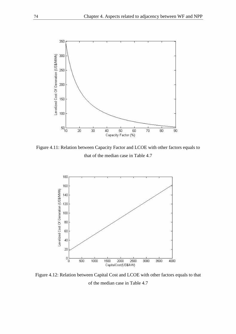
Chapter 4. Aspects related to adjacency between WF and NPP 74
Figure 4.11: Relation between Capacity Factor and LCOE with other factors equals to
that of the median case in Table 4.7
Figure 4.12: Relation between Capital Cost and LCOE with other factors equals to that
of the median case in Table 4.7

75 ( 4.5 Levelized Cost of Energy (LCOE
4.5.1 Comparing LCOE for Cases A & B and Scenarios I, II, &
III
LCOE will be calculated for different cases A & B, and different scenarios I, II, &
III which are described in section 4.1.1. Life time and discount rate will be the same for
all cases and scenarios. On the other hand, capacity factor and capital and operation &
maintenance costs are site and/or WT specific, therefore values of these parameters are
different for different cases and scenarios. As stated before, coupling of WFs with NPPs
has some advantages and disadvantages. Some of these advantages and disadvantages
are related to the economics of the WF, and they can be summarized in Table 4.8 with
the projected increase/decrease in capital and operation & maintenance costs compared
to median case. Other advantages and disadvantages are ignored as they do not have
direct economical impact, but they have technical one which cannot be translated to
economical impact. On the other hand, suitable site for coupling may have lower
capacity factor, and so lower energy production for a certain installed capacity,
compared to other potential sites in the country. This is clear in Figure 4.4, where case
A which represents the case of coupling has lower energy production compared to case
B. Therefore, to take a right decision which is better case A or B, the two cases have to
be compared considering all key parameters which affect the energy production costs.
This can be achieved by comparing LCOE for each case.
Applying Equations (4.9) to (4.17) to cases A & B, and considering the three
scenarios, Figures 4.13, 4.14, and 4.15 can be obtained. Each figure represents the
application of the two cases using one scenario. Any installations in Zafarana site, old or
new, have the same costs of median case in Table 4.7. Installations in El Dabaa site are
expected to have lower costs compared to Zafarana site (median case) due to coupling.
LCOE for the two cases A & B are calculated considering different levels of reduction
in capital cost and operation & maintenance cost for installations in El Dabaa site.
In Figures 4.13 to 4.15, LCOE for the two cases are drawn versus the capital cost
reduction (in percentage of the median case) for installations in El Dabaa site. Also, the
operation & maintenance cost reduction (in percentage of the median case) for
installations in El Dabaa site is taken as a parameter. It is clear that with no reduction in

Chapter 4. Aspects related to adjacency between WF and NPP 76
both types of cost, LCOE for case B is cheaper. This is applicable for all scenarios.
Considering Figure 4.13 (scenario I) LCOE for the two cases are equal when the capital
cost reduction is about 55%. Above this value of capital cost reduction or with any
reduction in the operation & maintenance cost, LCOE of case A will be cheaper. This is
applicable also for Figures 4.14 and 4.15 with slightly different values of capital cost
reduction required to achieve equality between the two cases. Therefore, for the
coupling (case A) to be feasibly from the economical point of view, it has to achieve the
required reduction in capital cost and/or operation and maintenance cost and so lower
LCOE or at least to be equal to that of case B.
Table 4.8 presents some aspects associated with coupling and their projected
increase/decrease in capital costs and/or operation & maintenance cost. It is based on
the previous illustration of whole advantages and disadvantages of coupling. According
to this table, coupling will decrease the operation & maintenance cost with about 10%,
and the decrease in capital cost ranges from 45% to 65%. Although there is a great
difference in the capacity fact between the two cases, expected reduction in costs is
sufficient to make LCOE for case A cheaper that of case B or at least both will be equal.
Therefore, the idea of coupling is economically feasible.

77 ( 4.5 Levelized Cost of Energy (LCOE
Figure 4.13: Scenario I: LCOE for cases A & B versus capital cost reduction (%) due to
coupling, with operation & maintenance cost reduction (%) as a parameter
Figure 4.14: Scenario II: LCOE for cases A & B versus capital cost reduction (%) due
to coupling, with operation & maintenance cost reduction (%) as a parameter

Chapter 4. Aspects related to adjacency between WF and NPP 78
Figure 4.15: Scenario III: LCOE for cases A & B versus capital cost reduction (%) due
to coupling, with operation & maintenance cost reduction (%) as a parameter
Table 4.8: Aspects related to coupling and their projected increase/decrease in costs of
electricity generation
+: increase, -: decrease, C: Capital Cost, O&M: Operation and Maintenance Cost
Aspect Projected +/ - in cost
+/- C/ O&M %
Availability of land with cheap prices - C 5
Existence of connection to grid - C 0 - 10
Existence of infrastructure required for WF - C 5
Smoothing effect of aggregated wind energy - O&M 10
Voltage variations at PCC - C 5
Reactive Power control capability - C 30 - 40
WF’s switch gear + C 5
Filters for WF’s produced harmonics + C 5

79
Chapter 5
Conclusions and Future Work
In this thesis, different aspects related to the coupling of WFs with NPPs are
studied. A brief literature survey on the previous research work related to this topic is
introduced. This is followed by discussing the basic criteria for selecting the site that
can accommodate both NPP and WF. This site selection criteria is then applied to
Egypt. There are sites in Egypt that passes the initial site selection requirements for both
NPP and WF. Next, the benefits of NPP and WF coupling are discussed. Also, some
disadvantages of coupling and the proper solution for each disadvantage are illustrated.
After that, some coupling advantages are chosen for more illustrations and
verifications with case studies. The benefits of connecting the WF and NPP to the same
point of the grid are illustrated; one of them is the elimination of the voltage quality
problems associated with the WF at the point of connection. The benefit of increasing
reliability and availability of NPP EPSs by the on-site WF is also illustrated. A study
using MARKOV process is conducted to quantify this increase in reliability and
availability.
After that, case studies are conducted to illustrate the effect of WFs geographical
distribution on the aggregated wind power production in the Egyptian grid along with
evaluating the wind energy capacity credit assessment.
Other future work can be done based on this work. This future work can be
summarized in the following points:
1. Studying the benefits of adding an energy storage facility to the system. It is
proposed to study in details the benefits (technical and economical) of adding an energy
storage facility, and choose the best technology of energy storage to be used in different
operating conditions.

Chapter 5. Conclusions and Future Work 81
2. Conducting simulations to study the benefit of coupling on the WF’s Low
Voltage Ride Through capability if a fault occurred at PCC. This is done by comparing
the results of different cases such as NPP and WF are in operation; NPP is shutdown,
while WF is in operation; and WF is connected to weak grid.
3. Studying the coupling of offshore WFs with NPPs. It is proposed to study
different aspects associated with this coupling including the usage of HVDC connection
to WF.

81
References
[1] Egyptian Electricity Holding Company, “Annual Report 2011/2012”
[2] Mohamed ElSobki and Peter Wooders, “Clean energy investment in developing
countries: Wind power in Egypt”, International Institute for Sustainable
Development (IISD), 2009
[3] Kate Rogers and Magdi Ragheb, “Symbiotic coupling of wind power and
nuclear power generation”, International Nuclear and Renewable Energy
Conference, Jordan, 2010
[4] Gregor Taljana, Michael Fowler, Claudio Canizares, and Gregor Verbic,
“Hydrogen storage for mixed wind–nuclear power plants in the context of a
hydrogen economy”, international journal of hydrogen energy 33, Elsevier,
2008
[5] Ahmed Shata, “Theoretical investigation and mathematical modeling of a wind
energy system: Case study for Mediterranean and Red Sea”, MSc thesis, der
Technischen Universität Berlin, 2008
[6] Mark Antkowiak, Richard Boardman, et al., “Summary Report of the INL-
JISEA Workshop on Nuclear Hybrid Energy Systems”, Technical Report
NREL/TP-6A50-55650, July 2012
[7] Alistair I. Miller & Romney B. Duffey, “Co-Generation of Hydrogen from
Nuclear
and Wind: the Effect on Costs of Realistic Variations in Wind Capacity and
Power Prices”, Atomic Energy of Canada Limited, 2005
[8] Charles W. Forsberg, “Sustainability by combining nuclear, fossil, and
renewable energy sources”, Progress in Nuclear Energy, Elsevier, 2008
[9] International Atomic Energy Agency, “Site evaluation for nuclear installations”,
Safety requirements, NS-R-3, 2003
[10] Andrew Macintosh, “Siting nuclear power plants in Australia”, Australian
institute for a just sustainable peaceful future, 2007
[11] L.R. Bishnoi and Prabir C. Basu, “Siting of Nuclear Installations”, Atomic
Energy Regulatory Board, India, 2005

References 81
[12] European Commission, “European best practice guidelines for Wind Energy
development”, Online:
http://ec.europa.eu/energy/res/sectors/doc/wind_energy/best_practice.pdf
[13] Auswind, “Best practice guidelines for implementation of wind energy projects
in Australia”, 2006.
[14] Egyptian Nuclear Power Plant Authority, “Egyptian nuclear power plant
program, history and status”, BULATOM Nuclear Conference, 2010.
[15] Niels G. Mortensen, Usama Said, and Jake Badger, “Wind atlas for Egypt”, Risø
National Laboratory, Egyptian New and Renewable Energy Authority, 2006.
[16] Pramod Jain, “Wind energy engineering”, McGraw-Hill Companies, 2011
[17] Baharat Atomic Research Center, “Health physics & environment”, BARC
Highlights, Reactor Technology & Engineering, 2007
[18] Thomas Ackermann, “Wind power in power systems”, John Wiley & Sons,
2005
[19] Deutsches Windenergie-Institut GmbH, Tech-wise A/S, DM Energy, ”Wind
turbine grid connection and interaction”, 2001
[20] Jonathan D. Rose and Ian A. Hiskens, “Challenges of integrating large amounts
of wind power”, 1st Annual IEEE Systems Conference, Hawaii, USA, 2007
[21] Tony Burton, David Sharpe, Nick Jenkins, Ervin Bossanyi, ”Wind energy
handbook”, John Wiley & Sons, Ltd, 2001
[22] Brendan Fox, Damian Flynn, et al., “Wind power integration, connection and
system operational aspects”, The Institution of Engineering and Technology,
2007
[23] World Bank Group, “Environmental, health, and safety guidelines for wind
energy”, 2007
[24] Alexandra Gadawski and Greg Lynch, “The Real Truth About Wind Energy: A
Literature Review on Wind Turbines in Ontario”, Sierra Club Canada Interns,
2011
[25] Australian Wind Energy Association, “Wind farm safety in Australia”, 2004
[26] M. Ragheb, “Safety of Wind Systems”, University of Illinois, 2012
[27] EDS Consulting, “Land Use Planning for Wind Energy Systems in Manitoba”,

83 References
2009
[28] Wind Energy , Defense & Civil Aviation Interests Working Group, “Wind
Energy and Aviation Interests-Interim Guidelines”, Crown Copyright, 2002
[29] Remus Teodorescu, Pedro Rodriguez, Andrzej Adamczyk “Reactive power
control for Wind Power Plant with STATCOM”, MSc Thesis, Institute of
Energy Technology, Aalborg University, Denmark, 2010
[30] Gonzalo Abad, Jesu´s Lo´pez, et al., “Doubly Fed Induction Machine- Modeling
and Control for Wind energy Generation”, Institute of Electrical and Electronics
Engineers, Inc., John Wiley & Sons, Inc, 2011
[31] Carson W. Taylor, “Power system voltage stability”, Electrical Power Research
Institute, 1994
[32] L. H. Hansen, L. Helle, et al., “Conceptual survey of Generators and Power
Electronics for Wind Turbines”, Risø National Laboratory, 2001
[33] Manfred Stiebler, “Wind energy systems for electric power generation”,
Springer-Verlag Berlin Heidelberg, 2008
[34] IEC Standard 61400-21, “Wind turbine generator systems – Part 21:
Measurement and assessment of power quality characteristics of grid connected
wind turbines”, Reference number CEI/IEC 61400-21:2001, 2001
[35] Cezary Szafron, "Wind Energy Conversion Systems Grid Connection", MSc
thesis, Wroclaw University of Technology, Poland, 2011
[36] Miller AI, Duffey RB, “Integrating large-scale co-generation of hydrogen and
electricity from wind and nuclear sources (NUWIND)”, IEEE EIC Climate
Change Technology, 2006
[37] Gregor Taljan, “The use of hydrogen in electric power systems”, PhD thesis,
University of Ljubljana, 2009
[38] International Atomic Energy Agency, “Electric grid reliability and interface with
nuclear power plants”, NG-T-3.8, 2012.
[39] International Atomic Energy Agency, “Interfacing Nuclear Power Plants with
the Electric Grid: the Need for Reliability amid Complexity”, Paper, online:
http://www.iaea.org/About/Policy/GC/GC53/GC53InfDocuments/English/gc53i
nf-3-att5_en.pdf

References 84
[40] International Atomic Energy Agency, “Design of Emergency Power Systems for
Nuclear Power Plants”, NS-G-1.8, 2004
[41] S.A. Eide, C.D. Gentillon, T.E. Wierman, D.M. Rasmuson, “Reevaluation of
Station Blackout Risk at Nuclear Power Plants”, Idaho National Laboratory,
NUREG/CR-6890, Vol. 2, 2005
[42] Mazaher Haji Bashi, Akbar Ebrahimi, “Markovian approach applied to
reliability modeling of a wind farm”, Turkish Journal of Electrical Engineering
& Computer Sciences, 2012
[43] D. J. Campbell, R. E. Battle, “Reliability of Emergency AC Power Systems at
Nuclear Power Plants”, NUREG/CR-2989, Jul 1983
[44] Yannick Degeilh, “Wind farm diversification and its impact on power system
reliability”, MSc thesis, Texas A&M University, USA, 2009
[45] Smith, J. C., Milligan, M. R., DeMeo, E. A., and Parsons, B. “Utility Wind
Integration and Operating Impact State of the Art,” IEEE Transactions on Power
Systems, 2007
[46] Sunanda Mishra, “Wind Power Capacity Credit Evaluation Using Analytical
Methods”, MSc thesis, University of Saskatchewan, Canada, 2010
[47] International Energy Agency, and Nuclear Energy Agency “Projected Costs of
Generating Electricity, 2010 Edition”, 2010.

شمس عين جامعة الهندسة كلية
الكهربية والآلآت القوي هندسة قسم
لطاقة النوويةة للرياح مع محطة لاقتران مزرع
رسالة مقدمة للحصول علي درجة الماجستير في الهندسة الكهربية
تخصص هندسة القوي و الآلات الكهربية من مقدمه
محمد كريم عبد الرحمن ابراهيم العشيري
الهندسة الكهربية بكالوريوس الكهربية والآلآت القوي هندسة قسم
8002، شمس عين جامعة
إشراف تحت
عبد الرحيم بدر محمد /د.ا د/ وليد علي سيف الاسلام الختام
مصطفي صالح القليل/ د
8002 ،القاهرة

شمس عين جامعة الهندسة كلية
الكهربية والآلآت القوي هندسة قسم
لطاقة النوويةة للرياح مع محطة لاقتران مزرع
من مقدمهماجستير ال للحصول علي درجة رسالة
محمد كريم عبد الرحمن ابراهيم العشيري
لجنة الحكم
التوقيع الاسم
أ.د. عصام الدين محمد أبو الذهب
قسم القوي و الآلات –كلية الهندسة –جامعة القاهرة الكهربية
................
أ.د. المعتز يوسف عبد العزيز محمد
الآلات و القوي قسم – الهندسة كلية – عين شمس جامعة الكهربية
................
أ.د. محمد عبد الرحيم بدر عميد كلية الهندسة و التكنولوجيا –جامعة المستقبل
................
أ.د. وليد علي سيف الاسلام الختام
الآلات و القوي قسم – الهندسة كلية – عين شمس جامعة الكهربية
................
8002التاريخ: / /

شمس عين جامعة الهندسة كلية
الكهربية والآلآت القوي هندسة قسم
ماجستير رسالة
محمد كريم عبد الرحمن ابراهيم العشيري : لطالبا اسم
الرساله عنوان
: النووية للطاقة محطة مع للرياح مزرعة اقتران
القوي و الألات هندسة) الكهربائية الهندسة في العلوم ماجستير : الدرجه اسم
الكهربية(
الاشراف لجنة
عميد كلية الهندسة و التكنولوجيا عبد الرحيم بدر محمد /د.أ
المستقبل جامعة
الكهربية الألات و القوي هندسة قسم د/ وليد علي سيف الاسلام الختام شمس عين جامعة -الهندسه كلية
هيئة الطاقة الذرية -مركز البحوث النووية مصطفي صالح القليل/ د
العليا الدراسات بتاريخ الرساله أجيزت الاجازه ختم
/ /8002
ةالكلي مجلس موافقة / /8002
الجامعه مجلس موافقة / /8002

تعريف بمقدم الرسالة
محمد كريم عبد الرحمن ابراهيم الاسم:
0826/ 6/ 82 تاريخ الميلاد:
المملكة العربية السعودية محل الميلاد:
الهندسة الكهربية، تخصص قوي و آلات كربية بكالوريوس الدرجة الجامعية:
جامعة عين شمس الجهة المانحة:
8002 المنح:تاريخ
معيد بهيئة الطاقة الذرية المصرية الوظيفة الحالية:

صخلمال
الدول تواجه التي التحديات أكبر من ةواحد يالمناخ تغيرال أصبحت قضية
يالمناخ تغيرال تهديداتمواجهة و تتطلب . العالم في المواطنين و والشركات والحكومات
لتقليل هائلة جهود هناك أيضا. الطاقة توليد مجموع من المتجددة الطاقة حصة في زيادة
استخدام لزيادة المجال يفتح الذي الأحفوري الوقود من الطاقة مصادر على الاعتماد
لتلبية( مصر مثل) البلدان من العديد تخططلهذا . النووية الطاقة مثل البديلة الموارد
) المتجددة الطاقات من كلل المساهمات زيادة طريق عن الكهرباءعلي المتزايدة الطلبات
.الكهرباء توليد في النووية ةوالطاق( الرياح طاقةبخاصة
، النووية الطاقة محطات و الرياح مزارع كلا من قعامو لتحديد التخطيط مرحلة في
موقع تحديد أثناء الاعتبار بعين تؤخذ التي الهامة الجوانب أحد. التحديات من العديد توجد
في راالبحمن تأخذ هذه المياهو وجود مياه للتبريد في الموقع، هومحطة الطاقة النووية
ناحية من. راالبح سواحل علىلذلك معظم محطات الطاقة النووية تقع . الحالات معظم
سرعات وجود هو المؤثر الرئيسي جانبال ، مزرعة الرياح موقع تحديد خلال ، أخرى
أنحاء مختلف في الساحلية المناطق من العديد. في الموقع في معظم أوقات العام جيدةرياح
مزرعة رياح و محطة للطاقة من كلا اقتران. لبناء مزرعة رياح المطلب بهذا توفي العالم
هذه في. أيضا عقباتكما أن لها ، كثيرة فوائد اله ينهمب المتاخمة أو موقعال نفس فيالنووية
و فوائدتم دراسة و تقييم ،في هذا المجال ةالعالمي الخبرة أساس على ، الأطروحة
تم القيام متاخمةال/ قترانالا مفهوممن للتحقق ذلككو. متاخمةال/ قترانالا هذا معوقات
.علي الشبكة الكهربية في مصر المختلفة الحالة دراساتبعض ب
تطلبات الشبكة رياح مع محطة للطاقة النووية، ماقتران مزرعة -- الدلالية الكلمات
الكهربية لربط مزرعة رياح، التوزيع الجغرافي لمزارع الرياح، القدرة الائتمانية لمزرعة
الرياح، العول و الاتاحية باستخدام سلسلة ماركوف

محتويات فصول الرسالة
مع الرياح مزارع اقتران معوقات و فوائد وتقييم تدور حول دراسة الأطروحة هذه
:التالي النحو على نظمت فصول خمسة إلىهذه الرسالة نقسمتو، النووية الطاقة محطات
يحتوي علي تعريف بفكرة اقتران مزارع الرياح مع محطات الطاقة : الأول الفصل
.الأطروحة مخططعرض لدافع من وراء هذه الفكرة، وكما أنه ناقش ا النووية.
للموضوع. ثم يوضح الدراسة الاسترجاعية الفصل هذا عرضي: الثاني الفصل
كما يقيم هذا الفصل خصائص الموقع الملائم لبناء مزرعة رياح و محطة للطاقة النووية.
مزايا شرح تم ، أخيراو . اقترانهذا تستوعب أن يمكن التيالمواقع المختلفة في مصر
مزارع الرياح مع محطات الطاقة النووية. اقتران وعيوب
نفسمحطة الطاقة النووية ب ومزرعة الرياح ربط فوائد يوضح: الثالث الفصل
رئيسيتين فائدتين من للتحقق حالة تيدراسكما يعرض نتائج . الكهربية الشبكةفي النقطة
تم تقييم تأثير ارتفاع مستوي الماس الكهربي عند نقطة الربط لمزرعة لهذا الاقتران.
حساب الزيادة في الاتاحية و كما تم الكهربي عند هذه النقطة. الجهد جودةالرياح علي
العول لنظم الطاقة في حالات الطواريء لمحطات الطاقة النووية عن طريق دمج مزرعة
الرياح المتواجدة في الموقع.
فيلمزارع الرياح الجغرافي التوزيعبالتفصيل الفائدة من يناقش: الرابع الفصل
لمزارع الرياح الجغرافي التوزيع تأثير لتوضيح حالة دراسةالكهربية . تم اجراء الشبكة
تقييم تم ذلك، بعد ا.لهعلى اجمالي الطاقة المولدة من هذه المزارع و التغيرات اللحظية
قترانلهذا الا ستراتيجيةا خطةتم وضع ، أيضاو . مصر في الرياح طاقةل الائتمانية القدرة
مزارع الرياح و محطات الطاقة النووية بين التنسيقأخذين في الاعتبار ، مصر في
التنافسية القدرة من للتحقق حالة دراسة إجراء تم ، أخيراالمخطط بناؤها في المستقبل.
من مزرعة رياح مجاورة لمحطة طاقة نووية في مصر. الطاقة توليد لتكلفة
بحثال وضع نقاطو الاستنتاجات استخراجب الأطروحةيختم هذه : الخامس الفصل
.العمل هذا بناءا على ابه القيام يمكن التي المستقبلية